Thermal dynamics on the lattice with exponentially improved accuracy

Abstract

We present a novel simulation prescription for thermal quantum fields on a lattice that operates directly in imaginary frequency space. By distinguishing initial conditions from quantum dynamics it provides access to correlation functions also outside of the conventional Matsubara frequencies $\omega_{n}=2\pi nT$. In particular it resolves their frequency dependence between $\omega=0$ and $\omega_{1}=2\pi T$, where the thermal physics $\omega\sim T$ of e.g. transport phenomena is dominantly encoded. Real-time spectral functions are related to these correlators via an integral transform with rational kernel, so their unfolding is exponentially improved compared to Euclidean simulations.

We demonstrate this improvement within a $0+1$-dimensional scalar field theory and show that spectral features inaccessible in standard Euclidean simulations are quantitatively captured.

Modern experiments ranging from heavy-ion collisions at RHIC and LHC Muller:2013dea ; 2016EPJP..131…52A to ultracold quantum gases Bloch:RevModPhys.80.885 explore the physics of strongly-correlated quantum systems across vastly separated temperature scales $(T\sim 10^{12}..10^{-9}K)$ 2012NJPh…14k5009A . A unifying aspect of these studies are thermal phenomena, such as the transport of conserved charges Heinz:2011kt ; Ryu:2015vwa ; Meyer:2007dy ; Kamikado:2013sia ; Haas:2013hpa ; Christiansen:2014ypa ; Aarts:2014nba ; Mages:2015rea ; Ding:2016hua ; Chien1504.02907 ; Cao:2010wa ; Enss:2010qh or the in-medium modification of heavy bound states Ding:2012sp ; Aarts:2014cda ; Kim:2014iga ; Borsanyi:2014vka ; Burnier:2015tda ; PhysRevLett.100.053201 ; Nishida:2008ra . Connecting these to fundamental interactions, such as QED and QCD, requires a thorough theoretical understanding of the equilibrium properties of quantum fields. Unfortunately in realistic experimental environments many approximate techniques, such as perturbation theory, are inapplicable and a non-perturbative numerical computation is required.

Conventional simulations of quantum fields, e.g. lattice QCD, are based on non-perturbative Monte-Carlo techniques relying on an analytic continuation of the real-time axis into the complex plane Foulkes:2001zz ; Smit:2002ug , for real-time approaches to spectral functions see e.g. Aarts:2001qa ; Strauss:2012dg ; Kamikado:2013sia ; Haas:2013hpa ; Tripolt:2013jra ; Haas:2013hpa ; Christiansen:2014ypa ; Helmboldt:2014iya ; Pawlowski:2015mia ; Yokota:2016tip ; Kamikado:2016chk ; Jung:2016yxl ; Ilgenfritz:2017kkp .

Two conceptual challenges plague the necessary reconstruction of real-time correlation functions from those simulated in imaginary time: the crucial one is the finite extent of the Euclidean time axis with $\tau\in[0\,,\,1/T]$. It leads to discrete Matsubara frequencies $\omega_{n}=2\pi nT$, which limits the resolution of imaginary frequencies. In turn, increasing the number of temporal points $N_{\tau}$ simply increases the maximum frequency available while keeping the spacing fixed. Thus, a large $N_{\tau}$ does not improve the access to the relevant regime $\omega\sim T$, where thermal physics is dominantly encoded in $G(\omega)$. The signal to noise ratio for thermal contributions actually decays rapidly above $\omega\approx T$ and indeed, already $G(\omega_{1}=2\pi T)$ may only be marginally relevant for thermal physics.

In order to resolve this conceptual issue, we present a simulation algorithm, which operates in imaginary frequency space with arbitrary resolution, given by the number of frequency points $N_{\omega}$. In particular this approach resolves frequencies between $\omega_{0}$ and $\omega_{1}$.

The second issue concerns the unfolding of spectral functions $\rho(\mu)$ from imaginary time correlators $G(\tau)$, or imaginary frequency correlators $G(\omega)$. In Euclidean time the inverse problem reads

$$G(\tau)=\int d\mu\,\tilde{K}(\mu,\tau,T)\rho(\mu),\quad\tilde{K}(\mu,\tau,T)\overset{\mu\tau>>1}{\sim}e^{-\mu\tau}\,.$$ (1)

Eq. (1) leads to an exponentially hard ill-posed problem JARRELL1996133 . In this work we simulate directly in imaginary frequency space, where numerical data and spectral functions are related via the rational Källén-Lehmann kernel,

$$G(\omega)=\int d\mu\,K(\mu,\omega)\rho(\mu),\quad|K(\mu,\omega)|\overset{\mu/\omega>>1}{\sim}\frac{1}{\mu/\omega}\,.$$ (2)

Its polynomial decay significantly improves the success of the spectral reconstruction already for Mastubara correlators with $\omega=\omega_{n}$. Such a rational kernel is moreover an analytic implementation of the idea behind the Backus-Gilbert Brandt:2015sxa or Sumudu Pederiva:2014qea approaches.

In summary, it is the combination of the rational kernel in (2) and the access to arbitrary frequencies that leads to exponentially improved accuracy in the spectral reconstruction, see Fig. 4 for the results.

Now we discuss the lattice setup that implements the above ideas. The starting point is a real-time thermal field theory, formulated on the Schwinger-Keldysh contour Berges:2006xc ; Berges:2015kfa . It amounts to an initial value problem with the following path integral representation for the partition function

$$\cal{Z}= \underbracket{\int_{\varphi_{E}(0)=\varphi_{E}(\beta)}{\cal D}\varphi_{E}e^{-S_{E}[\varphi_{E}]}}_{\rm initial\,conditions}\times$$

$$\hskip 28.45274pt\underbracket{\int_{\varphi^{+}(t_{0},{\bf x})=\varphi_{E}(0)}^{\varphi^{-}(t_{0},{\bf x})=\varphi_{E}(\beta)}{\cal D}\varphi e^{iS_{M}[\varphi^{+}]-iS_{M}[\varphi^{-}]}}_{\rm quantum\,dynamics},$$ (3)

with $S_{E}$ being the Euclidean- and $S_{M}$ the Minkowski space action. $\varphi$ lives on the forward and backward branch, $\varphi^{+}(t,{\bf x})$ lives on the forward branch from the inital time $t=t_{0}=-\infty$ to $t=\infty$, and $\varphi^{-}(t,{\bf x})$ lives on the backward branch, see Fig. 1. The initial conditions are expressed as a path integral for $\varphi_{E}(\bar{\tau},{\bf x})$ on a compact imaginary time axis $\bar{\tau}\in[0,\beta]$.

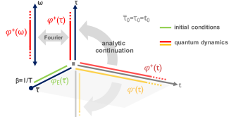
Figure 1: Sketch of the imaginary frequency setup.

Now we use that the real-time contour extends to infinity, and any correlations between fields at finite t and $t=+\infty$ vanish. This allows us to cut open the Keldysh contour at $t=+\infty$, and to rotate the real-time contour to an imaginary time axis, not to be confused with the time axis of the intial condition path integral. This rotation is implemented such that the path integrals for the rotated forward and backward branches have bounded statistical measures: the forward branch is rotated to the upper complex half plane while the backward branch to the lower one (see Fig. 1).

Furthermore, in equilibrium the correlator $G$ in (2) can be derived as the analytic continuation of the real-time correlator of the fields on the forward branch,

$$G^{++}(\omega):=\langle\varphi^{+}(\omega)\varphi^{+}(-\omega)\rangle\,.$$ (4)

Thus it suffices to compute the correlation functions on the forward contour, and we do not consider the backward contour any further here. The forward branch may now be treated using stochastic quantization Namiki:1992wf with a Euclidean action $S_{E}$. Its initial condition is given by the Euclidean field, $\varphi^{+}(\tau=t_{0})=\varphi_{E}(0)$, and the correlation function $G(\omega)$ can be computed for all $\omega\in\mathbb{R}$.

In practice the simulation is carried out on a finite temporal lattice with periodic boundary condition which introduces finite volume effects. We have checked that these lattice artefacts disappear in the infinite volume limit, but the convergence is very slow. A qualitatively enhanced convergence of both, infinite volume and continuum limit, can be achieved as follows: the Fourier transform to frequency space translates the initial condition to the constraint $\sum_{l}\varphi^{+}(\omega_{l})=\varphi_{E}(\bar{\tau}_{0})$, where $|l|=0,...,\lfloor N_{\omega}/2\rfloor$, and $\omega_{l}=2\pi l/(N_{\omega}\Delta\bar{\tau})$. Here $\Delta\bar{\tau}$ is the temporal lattice spacing on the standard Euclidean lattice. This constraint can be rewritten as one for the field at the highest frequency, $\varphi^{+}(\omega_{\lfloor N_{\omega}/2\rfloor})=\varphi_{E}(\bar{\tau}_{0})-\sum_{l}\varphi^{+}(\omega_{l})$. The kinetic term $1/2\sum_{l}\varphi^{+}(\omega_{l}){\cal P}(\omega_{l})\varphi^{+}(\omega_{l})$ with lattice dispersion $\cal P$ is local in frequency space. Firstly, the constraint is irrelevant in the continuum limit, as its statistical weight is vanishing due to $\varphi^{+}(\omega_{\lfloor N_{\omega}/2\rfloor}){\cal P}(\omega_{\lfloor N_{\omega}/2\rfloor})\varphi^{+}(\omega_{\lfloor N_{\omega}/2\rfloor})\to\infty$. Secondly, in the infinite volume we have an infinite number of momentum modes. This entails that the weight of one specific momentum mode tends towards zero. In summary, the dependence of the kinetic term on the inital condition is a well-understood lattice artefact. In the spirit of improved lattice actions we can lift the Matsubara constraint for all terms in the lattice action that are local in frequency space. Here we apply this reasoning to $S_{0}$, the quadratic part of the action. The efficient convergence of this approach is confirmed for the propagator, see Fig. 3.

The full theory is then formulated in a mixed representation in $\tau$ and $\omega$. While $S_{0}$ is simulated in $\omega$-space, $S_{\rm int}=S-S_{0}$ is directly implemented via a discrete Fourier transform in $\tau$-space, since interactions are local on the sites. Approximating the convolutions in the interaction term via DFT introduces a finite volume artifact, which vanishes as $N_{\omega}\to\infty$. The thermal initial condition $\varphi^{+}(\tau_{0})=\varphi_{E}(\bar{\tau}_{0})$ solely enters via this interaction term. This concludes the formulation and discussion of our lattice setup.

Our novel approach is now tested in a $0+1$ dimensional scalar field theory at temperature $T=1/\beta$, whose Euclidean action reads

$$S_{E}=\int d\tau\big{(}\underbracket{\frac{1}{2}(\partial_{\tau}\varphi_{E})^{2}+\frac{1}{2}m^{2}\varphi_{E}^{2}}_{S_{E}^{0}}+\underbracket{\frac{\lambda}{4!}\varphi_{E}^{4}}_{S_{E}^{\rm int}}\big{)}\,.$$

The system is simulated on a frequency lattice with $N_{\omega}$ points using stochastic quantization in Langevin time s,

$$\partial_{s}\varphi^{+}(\omega_{l})=-\frac{\delta S_{0}}{\delta\varphi^{+}(\omega_{l})}-\frac{\delta S_{E}^{\rm int}}{\delta\varphi^{+}(\tau_{j})}\frac{\delta\varphi^{+}(\tau_{j})}{\delta\varphi^{+}(\omega_{l})}+\eta(\omega_{l})\,.$$ (5)

Here a sum over $j=1,...,N_{\omega}$ is implied and the dispersion reads ${\cal P}(\omega_{l})=(2-2{\rm cos}[2\pi l/N_{\omega}])/\Delta\bar{\tau}^{2}$, $l\in[0,N_{\omega}-1]$. In (5) $\eta(\omega_{l})$ is the Fourier transform of the Gaußian noise, $\langle\tilde{\eta}(\tau_{i})\tilde{\eta}(\tau_{j})\rangle=\,2\delta_{ij}/\Delta\bar{\tau}$ and $S_{0}$ represents the discretized free action,

$$S_{0}=\sum_{l}\Delta\omega\;\frac{1}{2}\big{(}{\cal P}(\omega_{l})+m^{2}\big{)}|\varphi^{+}(\omega_{l})|^{2}\,,$$ (6)

while $S_{E}^{\rm int}=S_{E}-S_{0}$ is the interaction term. Concurrently we sample the thermal initial conditions at $N_{\tau}$ points along the compactified Euclidean time $\tau$,

$$\partial_{s}\varphi_{E}(\bar{\tau}_{k})=\frac{-\delta S_{E}}{\delta\varphi_{E}(\bar{\tau}_{k})}+\eta(\bar{\tau}_{k}),\;\langle\eta(\bar{\tau}_{i}),\eta(\bar{\tau}_{j})\rangle=2\frac{\delta_{ij}}{\Delta\bar{\tau}}\,.$$ (7)

so that the value of $\varphi^{+}(\tau=\tau_{0})$ can be replaced with $\varphi_{E}(\bar{\tau}=\bar{\tau}_{0})$ each time when computing $\frac{\delta S_{E}^{\rm int}}{\delta\varphi^{+}(\tau_{j})}$ in (5). After $\Delta s=1$ we record the correlators $G_{E}(\bar{\tau})=\langle\varphi_{E}(\bar{\tau})\varphi_{E}(0)\rangle$ and $G^{++}(\omega)=\langle\varphi^{+}(\omega)\varphi^{+}(-\omega)\rangle$, collecting in total $N_{\rm conf}=10^{6}$ samples, which leads to a relative statistical error $\Delta G/G\sim 10^{-3}$.

To crosscheck our computations we have also performed an equivalent quantum mechanical (QM) computation of the thermal real-time correlation functions $G^{\rm QM}(t)\equiv\langle\hat{x}(t)\hat{x}(0)\rangle$ using the anharmonic oscillator in the truncated Hilbert space of $32$ energy eigenfunctions of the harmonic oscillator Berges:2006xc . The spectral function is obtained from a Fourier transform of ${\rm Im}[\langle\hat{x}(t)\hat{x}(0)\rangle]$ along $N_{t}=3.2\times 10^{4}$ steps of $\Delta t=0.05$, i.e. it is computed only over a finite real-time extent. Due to the restricted Hilbert space and integration this computation underestimates the height of delta-peak like structures, present e.g. in the free spectrum and contains ringing.

In Fig. 2 we show the Euclidean correlators computed for the thermal scalar system at $\beta=1$ and $m=1$ along the standard compactified Euclidean axis for the free $\lambda=0$ (top points) and the interacting case $\lambda=24$ (bottom points). The black crosses denote the outcome of the QM computation and open symbols denote lattice results. For the free case we only carry out simulations at $N_{\bar{\tau}}=16$, while at $\lambda=24$ we produce data at four different $N_{\bar{\tau}}=16\ldots 128$. The inset shows the relative difference between the interacting correlator at $N_{\bar{\tau}}=16$ computed from the lattice and via quantum mechanics. For our choice of $ds=10^{-4}$ they agree within the statistical errors of the lattice simulation. Note that increasing $N_{\bar{\tau}}$, i.e. a smaller $\Delta\bar{\tau}$, leads to a larger drift term, so that at $N_{\bar{\tau}}=128$ the $ds$ needs to be reduced by two orders of magnitude to maintain an accurate outcome.

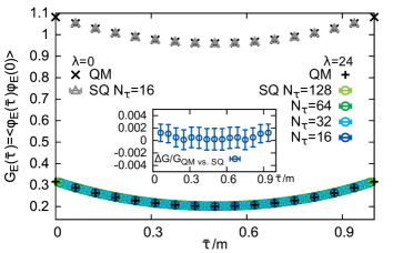
Figure 2: Euclidean correlation functions $G_{E}(\bar{\tau})$ for $\lambda=0$ (upper points) and $\lambda=24$ (lower points). Black crosses denote correlators from a quantum mechanical computation, while open symbols represent standard lattice simulations. The inset shows the relative difference between the lattice result for $\lambda=24$ at $N_{\bar{\tau}}=16$ and the quantum mechanical computation.

We focus on simulations with $N_{\bar{\tau}}=16$, and inspect the corresponding correlation functions in imaginary frequency space given in the top panel of Fig. 3 for both the free (gray) and interacting (colored) case. We show only the relevant low frequency regime up to $\omega/m=15$ while the simulations reach up to $\omega_{8}/m\approx 50$. As $\varphi^{+}(\tau)\in\mathbb{R}$ the correlators are real and symmetric around $\omega=0$.

The black filled symbols denote the correlators obtained from simply Fourier transforming the fields along the compact Euclidean domain and thus are located at the Matsubara frequencies $\omega_{n}$. The open symbols are obtained from the fields simulated directly along the imaginary frequency domain using between $N_{\omega}=16\ldots 512$ points. In the free $\lambda=0$ case our novel simulation yields a smooth interpolation between the Matsubara frequencies and furthermore as can be seen from the gray points in the lower panel of Fig. 3 agrees excellently with the values obtained from the Fourier transform of the compact Euclidean domain. Note that at $\lambda=0$ the two concurrent simulations (5) and (7) are completely decoupled.

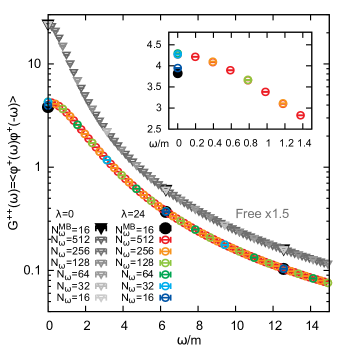
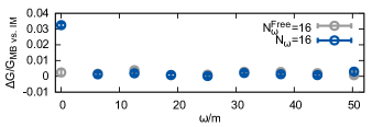
Figure 3: (top) Imaginary frequency correlators $G^{++}(\omega)$ from lattice simulations at $\lambda=0$ (gray, shifted $\times 1.5$) and at $\lambda=24$ (colored). Black filled symbols correspond to the correlator at the Matsubara frequencies accessible in standard simulations. Open symbols arise from our imaginary frequency simulation. The inset shows the low frequency regime at $\lambda=24$, in particular that finite volume artifacts are present at $\omega_{0}$ in the Matsubara correlator, which are removed going to finer resolution in $\omega$. (bottom) Relative difference standard Matsubara correlators and those from our direct simulation. Note the excellent agreement except for $\omega_{0}$ at $\lambda=24$, reflecting finite volume artifacts in the standard Matsubara value.

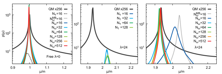
Figure 4: Spectral functions of the free theory (left) and at $\lambda=24$ unfolded from Euclidean (center) and imaginary frequency correlators (right). In each panel $\rho(\mu)$ from the corresponding quantum mechanical computation is plotted as solid thick gray line. Spectra denoted by $N_{\tau}$ are reconstructed from Euclidean correlators and $N_{\omega}^{\rm MB}$ from the Fourier transformed Matsubara one. The label $N_{\omega}$ refers to spectra from the direct imaginary frequency simulation resolving between $\omega_{n}$.

In the interacting case denoted by colored open symbols in Fig. 3, we again find a smooth interpolation between Matsubara frequencies and very good agreement with the standard Matsubara propagators for $\omega_{n>0}$. Let us inspect the regime close to the origin, given by the inset on the top of Fig. 3. Already at $N_{\omega}=16$ the new simulation (dark blue) leads to a value at $\omega=0$ that differs from the conventional Matsubara one (black). Increasing $N_{\omega}$ quickly lets the correlator converge significantly above the standard estimate. Since in a lattice simulation $\omega=0$ reflects the sum over all corresponding imaginary time extent, we infer that the standard simulation along the compactified Euclidean domain is not able to capture all the relevant late Euclidean-time physics that however can be vital to thermal processes. Its purpose is only to correctly sample $\varphi(\bar{\tau}_{0})$, which it does.

Now we extract spectral functions from the correlators, with kernels $\tilde{K}(\mu,\bar{\tau},T)={\rm cosh}[\mu(\bar{\tau}-/2T)]/{\rm sinh}[\mu/2T]$ and $K(\mu,\omega)=\frac{2\mu}{\mu^{2}+{\cal P}(\omega)}$. The latter is the lattice analogue of the continuum Källén-Lehmann kernel, and its use leads to a more efficient convergence of the spectral reconstruction. Here we deploy a recent Bayesian reconstruction (BR) method Burnier:2013nla and discretize positive real-time frequencies $\mu\in[10^{-3},200]$ with $N_{\mu}=4000$ points including a high frequency window of $N_{\mu}^{\rm HP}=1000$ around the lowest lying peaks. For minimal bias we use a flat default model $m(\mu)=1$. In the free case we know that only a single delta-peak at the mass of the field exists in the spectrum. The quantum mechanical computation given by the thick gray line in the left panel of Fig. 4 while being able to capture the position of the peak, gives an artificial finite width due to the underlying finite real-time extent Fourier transform. We have checked that it can be reduced systematically and therefore for visualization purposes multiply the curve here by a factor of 256. The reconstruction from the $N_{\bar{\tau}}=16$ compact Euclidean domain (dark gray dashed) both gives a too large width and its position is still slightly off. A Fourier transform of the Euclidean fields and reconstructing along Matsubara frequencies already improves the results significantly. The light gray dashed line shows a much reduced width and is positioned very close to unity. Since here the standard Matsubara data already leads to a very good result, the improvement from using the correlators of the new simulation only leads to a further decrease in the reconstructed width. Note that the width depends on the error of the data and can be improved by more statistics.

Turning to the interacting case $\lambda=24$, we first carry out the reconstruction from Eucldiean data, using different resolutions along $\bar{\tau}$. In the center panel of Fig. 4 the results are shown for $N_{\bar{\tau}}=16\ldots 128$. We find that the reconstruction does not capture the position of the lowest lying peak in the spectrum and even more importantly does not show a systematic improvement with $N_{\bar{\tau}}$. The reason is that with larger $N_{\bar{\tau}}$ higher $\omega_{n}$ become accessible but contribute only marginally to the relevant physics.

If on the other hand we use data in imaginary frequency space the situation is very different as shown in the right panel of Fig. 4. Again simply using the standard Matsubara correlators already improves the width of the reconstruction while the peak position is still off (gray dashed). However the access to the correlator at frequencies between $\omega_{0}$ and $\omega_{1}$ allows us to systematically and significantly improve the reconstruction of the lowest lying peak, with $N_{\omega}=512$ reproducing the peak position with high accuracy.

In summary we have shown that by carefully distinguishing initial conditions from quantum dynamics it is possible to devise a simulation prescription for thermal quantum fields along general imaginary frequencies. In particular this approach gives access to the thermal physics between $\omega_{0}$ and $\omega_{1}$. Real-time spectral functions are related to imaginary time correlators via an integral transform with a rational kernel, and in combination their extraction becomes exponentially improved. The success of this approach has been demonstrated here with scalar fields. It can be straightforwardly extended to Abelian and non-Abelian gauge theories which is work in progress. Evidently, computations of phenomenologically relevant quantities such as transport coefficients and heavy quark spectral functions will be improved significantly with our simulation prescription.

We thank N. Christiansen and S. Flörchinger for discussions. A.R. acknowledges fruitful exchanges with P. de Forcrand and A. Kurkela at CERN and during the ECT* workshop on advances in transport. This work is supported by EMMI, the grants ERC-AdG-290623, BMBF 05P12VHCTG. It is part of and supported by the DFG Collaborative Research Centre ”SFB 1225 (ISOQUANT)”.

References

- (1) B. Mueller, Phys. Scripta T158, 014004 (2013), 1309.7616.
- (2) N. Armesto and E. Scomparin, European Physical Journal Plus 131, 52 (2016), 1511.02151.
- (3) I. Bloch, J. Dalibard, and W. Zwerger, Rev. Mod. Phys. 80, 885 (2008).
- (4) A. Adams, L. D. Carr, T. Schäfer, P. Steinberg, and J. E. Thomas, New Journal of Physics 14, 115009 (2012), 1205.5180.
- (5) U. Heinz, C. Shen, and H. Song, AIP Conf. Proc. 1441, 766 (2012), 1108.5323.
- (6) S. Ryu et al., Phys. Rev. Lett. 115, 132301 (2015), 1502.01675.
- (7) H. B. Meyer, Phys. Rev. Lett. 100, 162001 (2008), 0710.3717.
- (8) K. Kamikado, N. Strodthoff, L. von Smekal, and J. Wambach, Eur. Phys. J. C74, 2806 (2014), 1302.6199.
- (9) M. Haas, L. Fister, and J. M. Pawlowski, Phys.Rev. D90, 091501 (2014), 1308.4960.
- (10) N. Christiansen, M. Haas, J. M. Pawlowski, and N. Strodthoff, Phys. Rev. Lett. 115, 112002 (2015), 1411.7986.
- (11) G. Aarts et al., JHEP 02, 186 (2015), 1412.6411.
- (12) S. W. Mages, S. Borsányi, Z. Fodor, A. Schaefer, and K. Szabó, PoS LATTICE2014, 232 (2015).
- (13) H.-T. Ding, O. Kaczmarek, and F. Meyer, Phys. Rev. D94, 034504 (2016), 1604.06712.
- (14) C.-C. Chien, S. Peotta, and M. Di Ventra, Nat Phys 11, 998 (2015).
- (15) C. Cao et al., Science 331, 58 (2011), 1007.2625.
- (16) T. Enss, R. Haussmann, and W. Zwerger, Annals Phys. 326, 770 (2011), 1008.0007.
- (17) H. T. Ding et al., Phys. Rev. D86, 014509 (2012), 1204.4945.
- (18) G. Aarts et al., JHEP 07, 097 (2014), 1402.6210.
- (19) S. Kim, P. Petreczky, and A. Rothkopf, Phys. Rev. D91, 054511 (2015), 1409.3630.
- (20) S. Borsanyi et al., JHEP 04, 132 (2014), 1401.5940.
- (21) Y. Burnier, O. Kaczmarek, and A. Rothkopf, JHEP 12, 101 (2015), 1509.07366.
- (22) E. Wille et al., Phys. Rev. Lett. 100, 053201 (2008).
- (23) Y. Nishida, Phys. Rev. A79, 013629 (2009), 0811.1615.
- (24) W. M. C. Foulkes, L. Mitas, R. J. Needs, and G. Rajagopal, Rev. Mod. Phys. 73, 33 (2001).
- (25) J. Smit, Cambridge Lect. Notes Phys. 15, 1 (2002).
- (26) G. Aarts and J. Berges, Phys. Rev. D64, 105010 (2001), hep-ph/0103049.
- (27) S. Strauss, C. S. Fischer, and C. Kellermann, Phys.Rev.Lett. 109, 252001 (2012), 1208.6239.
- (28) R.-A. Tripolt, N. Strodthoff, L. von Smekal, and J. Wambach, Phys.Rev. D89, 034010 (2014), 1311.0630.
- (29) A. J. Helmboldt, J. M. Pawlowski, and N. Strodthoff, Phys.Rev. D91, 054010 (2015), 1409.8414.
- (30) J. M. Pawlowski and N. Strodthoff, Phys. Rev. D92, 094009 (2015), 1508.01160.
- (31) T. Yokota, T. Kunihiro, and K. Morita, PTEP 2016, 073D01 (2016), 1603.02147.
- (32) K. Kamikado, T. Kanazawa, and S. Uchino, (2016), 1606.03721.
- (33) C. Jung, F. Rennecke, R.-A. Tripolt, L. von Smekal, and J. Wambach, (2016), 1610.08754.
- (34) E.-M. Ilgenfritz, J. M. Pawlowski, A. Rothkopf, and A. Trunin, (2017), 1701.08610.
- (35) M. Jarrell and J. Gubernatis, Physics Reports 269, 133 (1996).
- (36) B. B. Brandt, A. Francis, H. B. Meyer, and D. Robaina, Phys. Rev. D92, 094510 (2015), 1506.05732.
- (37) F. Pederiva, A. Roggero, and G. Orlandini, J. Phys. Conf. Ser. 527, 012011 (2014).
- (38) J. Berges, S. Borsanyi, D. Sexty, and I. O. Stamatescu, Phys. Rev. D75, 045007 (2007), hep-lat/0609058.
- (39) J. Berges, (2015), 1503.02907.
- (40) M. Namiki et al., Lect. Notes Phys. M9, 1 (1992).
- (41) Y. Burnier and A. Rothkopf, Phys. Rev. Lett. 111, 182003 (2013), 1307.6106.