Billiards in near rectangles

1 Introduction

Inside a polygonal billiard table, a billiard ball travels in straight line until it hits an edge. The billiard ball bounces off an edge obeying the law of reflection, i.e. the angle of incidence equals the angle of reflection. See Figure 1.

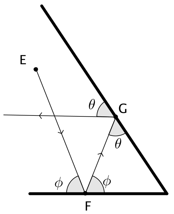
Figure 1: Law of Reflection

The trajectory of the billiard ball is called a billiard path. The path is periodic if the ball repeats the same path over and over again. We ignore cases where the billiard ball hits one of the vertices of the billiard table.

One major question in this subject is the following: Does every polygon admit a periodic billiard path? It is known that all polygons whose angles are rational multiple of $\pi$ have a periodic billiard path, see [1] and [3]. Schwartz has shown that all triangles with all angles smaller than 100 degree have periodic billiard path [4], [5]. In another paper by Hooper and Schwartz, it is shown that all triangles near enough to isosceles triangles have periodic billiard paths [2].

In this paper, we consider quadrilaterals which are close to being rectangles. The space $\mathcal{Q}$ of quadrilaterals (modulo similarity) can be “considered” as a subset of the $\mathbb{R}^{4}$, see Section  2.2. The main result of this paper is the following:

Theorem 1.

For every rectangle $r\in\mathcal{Q}$, there exists an open neighborhood $U\subset\mathcal{Q}$ containing $r$, such that every quadrilateral in $U$ has a periodic billiard path.

Theorem  2.2.4 will provide an explicit neighborhood $U$ for the special case when $r$ is a square.

Figure 2: Right Triangle

2 Preliminary

2.1 Tools for Studying Billiards

Consider a right triangle in Figure  2. Suppose the billiard ball starts from point $D$ moving upwards, perpendicular to side $BC$. Then it will hit the point $E$, reflect to hit point $F$, and then reflect to hit point $G$. We will leave it to the reader to show that $\angle x=\frac{\pi}{2}$.

The implication is that: after the ball hit $G$, it would bounce back along the exact same trajectory, and continues periodically. So, all right triangles have this periodic billiard path.

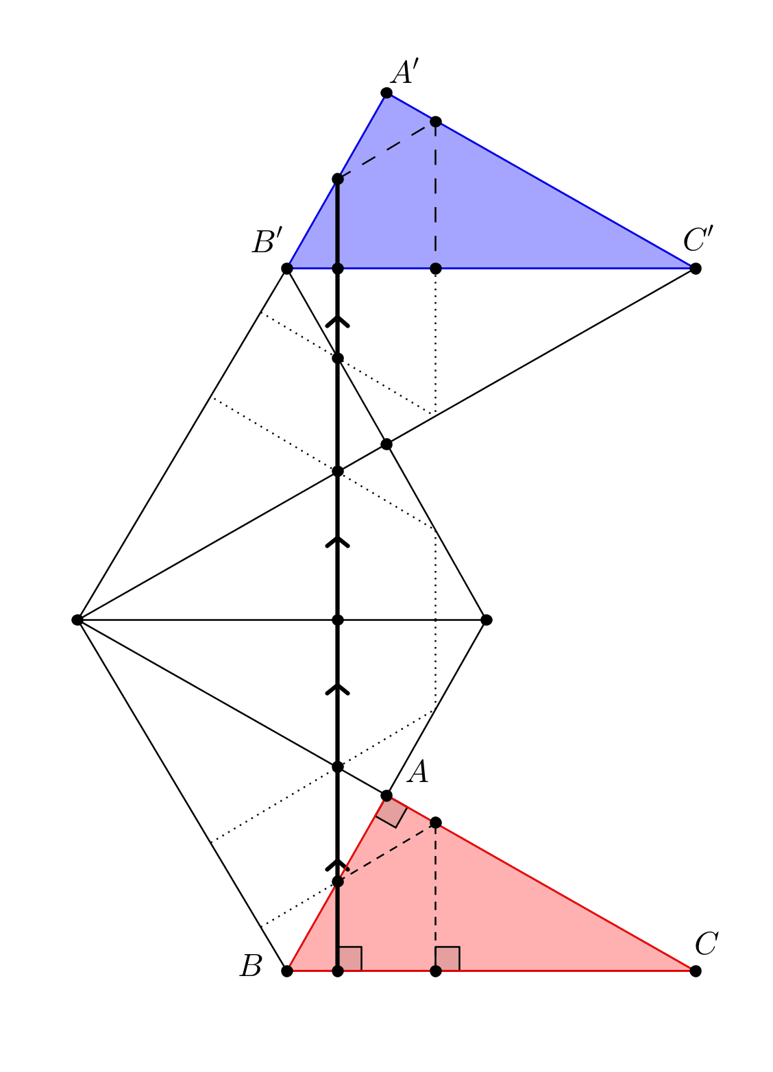
Figure 3: Unfolding for right triangle

If we label the sides $CB,BA,AC$ using $0,1,2$ respectively, then the sequence $012021$ represents the order in which the trajectory hits the sides of the polygon. We call this finite sequence the orbit type of the periodic path, and the length of the orbit type (in the example above, 6) the combinatorial length.

A very useful tool to study billiard paths is the unfolding. See [6] also.

Definition 2.1.1.

Given any orbit type $W=w_{1}w_{2}w_{3}\ldots w_{n}$, and any polygon $P$, the corresponding unfolding is a sequence of polygons $U(W,P)=P_{0}P_{1}P_{2}\ldots P_{n}$, such that $P_{0}=P$, and each $P_{j}$ is obtained by reflecting $P_{j-1}$ along the edge $w_{j}$ for $j\geq 1$.

For example, in Figure  3, each time the ball hits an edge of the polygon, instead of reflecting the billiard path, we reflect the polygon and keep the path straight. The straight line in the unfolding will “correspond” to the original periodic path. Note that the two shaded triangles in Figure  3 are related by a translation along the direction of the billiard trajectory. Also, this translation requires a number of 6 reflection, which is exactly the combinatorial length of the orbit.

Figure 4: Fagnano Path

Next, let us look at the famous Fagnano orbit. For any acute triangle, we can connect the three feet of the altitudes, as in Figure  4. Then the orbit $XY,YZ,ZX$ is actually a periodic billiard path. The proof is as follows:

Clearly points $X,Y,B,O$ lies on a circle, and $A,X,O,Z$ on another circle. So $\alpha=\theta=\gamma=\beta$. Hence, the path obey the law of reflection at the point $X$, and similarly at $Y,Z$.

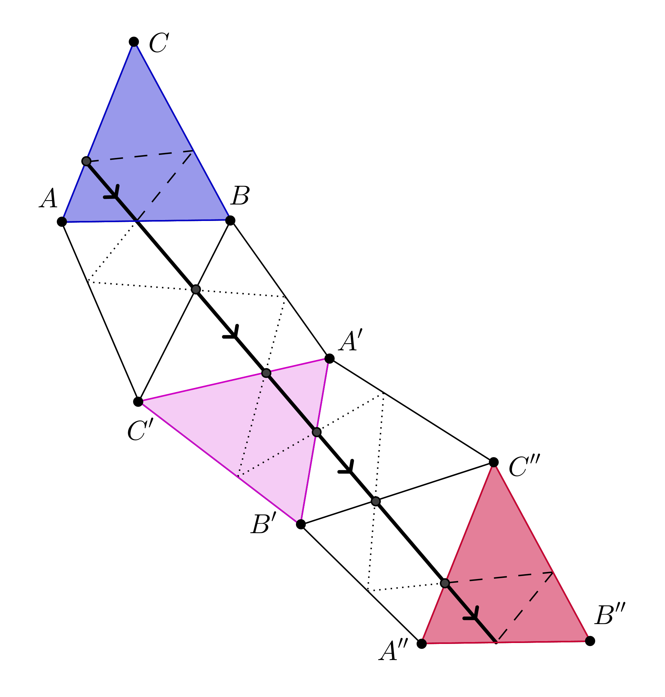
Figure 5: Unfolding for Fagnano path

By labelling $AB,BC,CA$ using $0,1,2$ respectively, we can “represent” this periodic path by the word $012$ (which has length 3). However, after 3 reflections in the unfolding(see Figure 5), the resultant polygon ($A^{\prime}B^{\prime}C^{\prime}$) is not a translation of the original polygon ($ABC$).

The reason is that each reflection of the polygon changes its orientation. In order to have a translation, we need an even number of reflections. So if a periodic path can be “represented” by a word $P$ of odd length (in the example above, $012$), then we define its orbit type to be $P^{2}$($012012$), so that the first polygon ($ABC$) and last polygon ($A^{\prime\prime}B^{\prime\prime}C^{\prime\prime}$) in the unfolding are related by a translation.

Of course, we can always reflect a polygon according to some arbitrary word. Then one important question is, given a word $W$, can we always find a corresponding periodic billiard path in some given polygon $P$? We have the following Lemma:

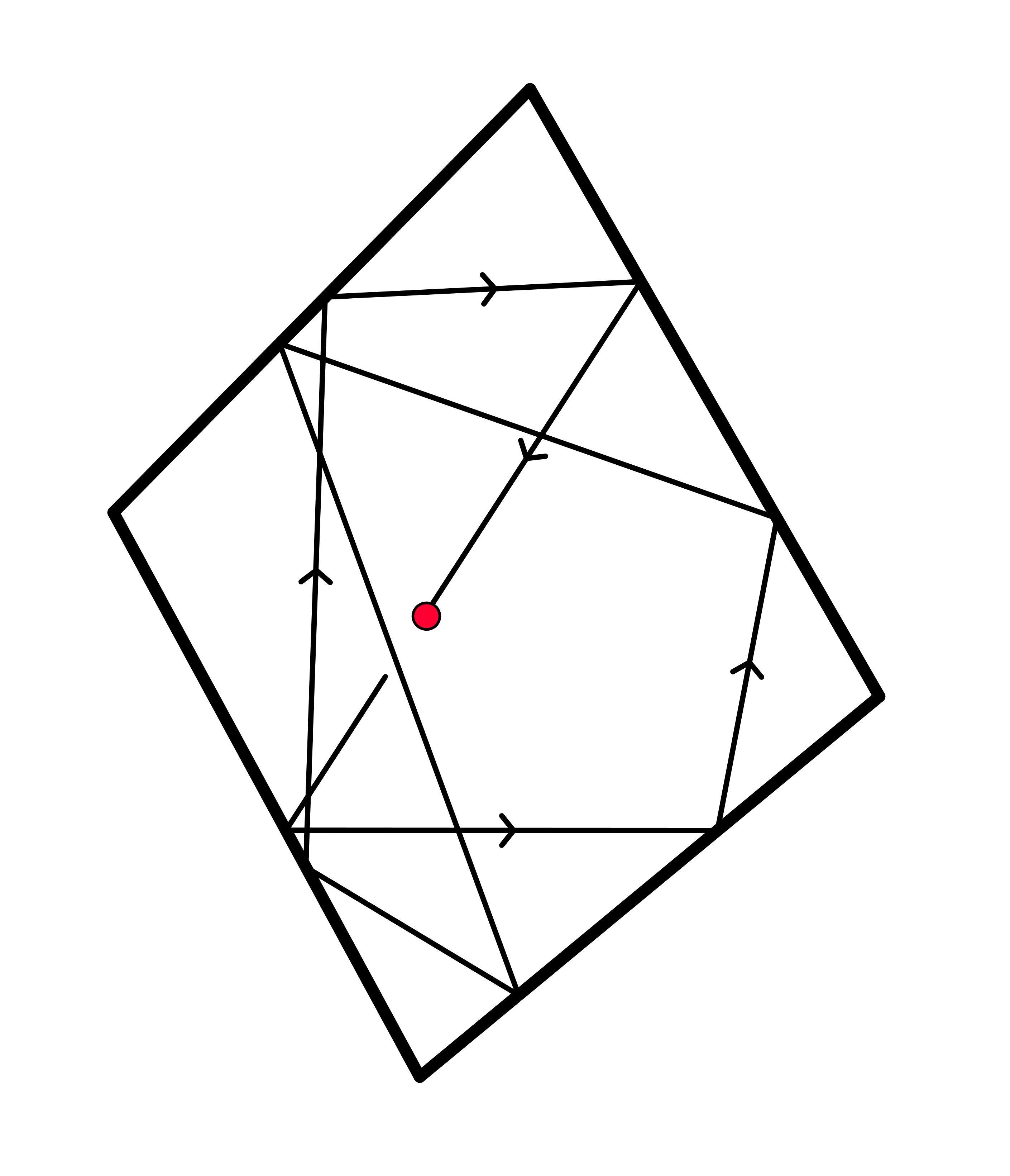
(a)

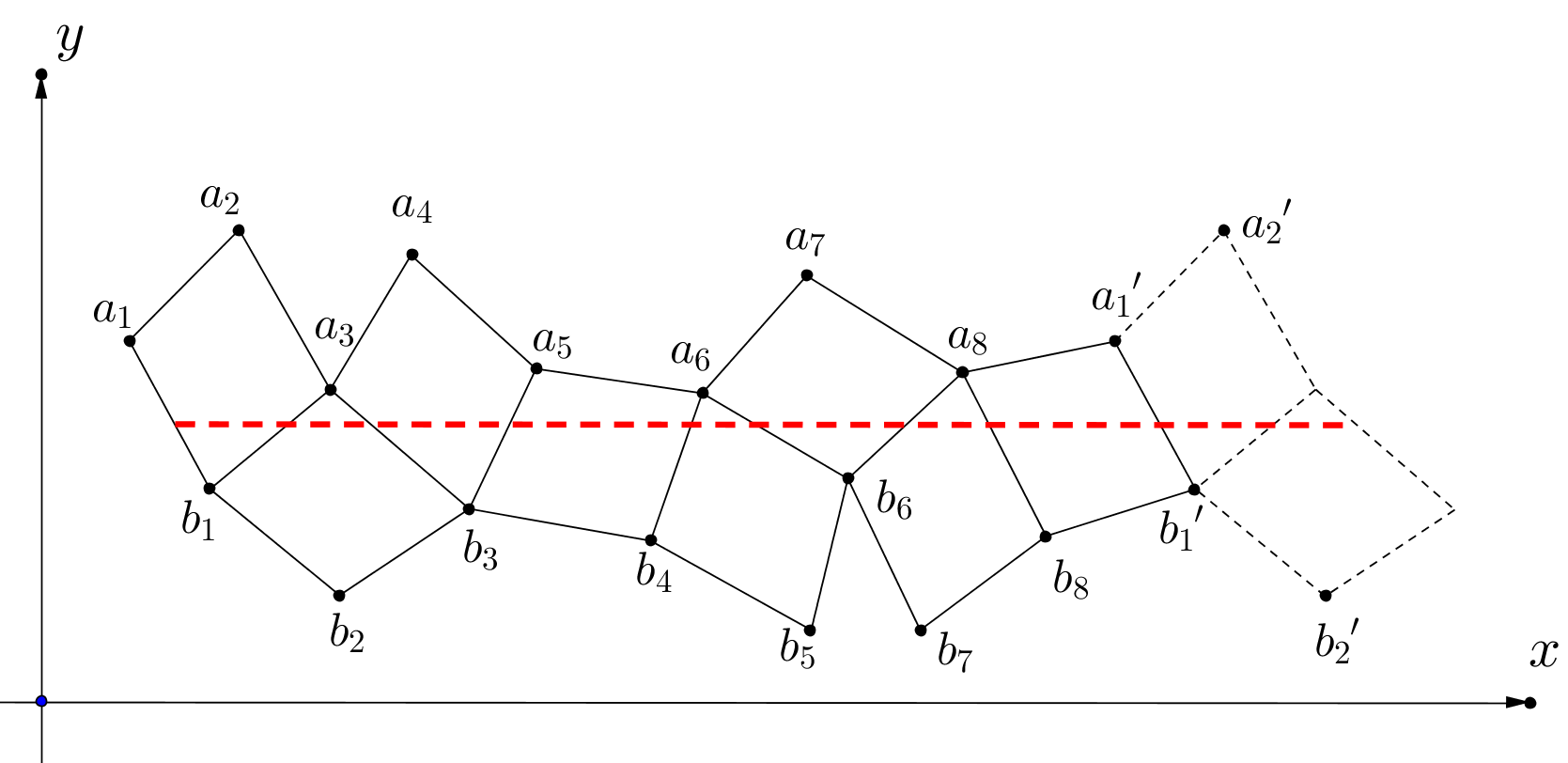
(b)

Figure 6:

Lemma 2.1.2.

For an even word $W$ and a polygon $P$, there exists a periodic billiard path on $P$ with the orbit type $W$ if and only if:

1. The first and the last polygon in the unfolding $U(W,P)$ are related by a translation. AND

2. There exists a straight line segment, parallel to the direction of the translation, that stays within the unfolding and does not touch any of the vertex.

To illustrate the second condition, let’s look at Figure  6b, which is the unfolding for the periodic billiard path in Figure  6a. Assuming Condition 1 is satisfied, then a polygon has this periodic billiard path if and only if we can “fit” the red dashed line into the corresponding unfolding. (i.e. in Figure  6b, if we choose the direction of the translation as our $x$-axis, then we need the $y$-coordinate of $a_{i}$ to be larger than that of $b_{j}$ for any $i$ and $j$.)

2.2 The space of quadrilaterals

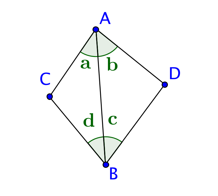
Figure 7: Four Parameters

Consider the space of all quadrilaterals (up to similarity), call it $\mathcal{Q}$. For any quadrilateral, we can split it into two triangles by drawing a diagonal. Each triangle is uniquely determined by two of its angles. So, any quadrilateral is determined by four parameters, $a,b,c,d$, as shown in Figure 7. The parameters of the square are $(\frac{\pi}{4},\frac{\pi}{4},\frac{\pi}{4},\frac{\pi}{4})$, and rectangles are on the line

$\{(a,b,c,d):a=c,b=d,a+b=\frac{\pi}{2}\}$.

For each orbit type $W$, we call the set of all quadrilaterals with this orbit type the orbit tile $O(W)$ of the orbit type.

Definition 2.2.1.

A orbit type $W$ is called stable if the orbit tile $O(W)$ is a nonempty open set. Otherwise, $W$ is unstable.

We will use the following criterion for the stability of an orbit type. See [6]

Lemma 2.2.2.

For $O(W)\neq\emptyset$, an orbit type W is stable if and only if the number of times each sides of the polygon appears in an odd position in the orbit type equals the number of times it appears in an even position.

For example, the orbit type $012021$ is not stable, because $1$ appears twice in even positions (and does not appear at odd position). Also, $012012$ is stable.

Now we shall restate our main theorems more precisely.

Definition 2.2.3.

For $\varepsilon>0$, a quadrilateral with parameter $(a_{1},a_{2},a_{3},a_{4})$ is called $\varepsilon$-near square if $\left|a_{i}-\frac{\pi}{4}\right|<\varepsilon$ for any $i$.

Theorem 2.2.4.

The set of all $\frac{\pi}{107}$-near square quadrilaterals is covered by finitely many orbit tiles.

Theorem 2.2.5.

An open neighborhood of the rectangle line in the space $\mathcal{Q}$ can be covered by finitely many orbit tiles.

3 Proof of Theorem  2.2.4

3.1 $\alpha$-$\beta$ plane

(a)

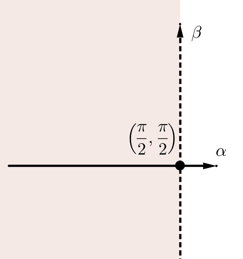
(b)

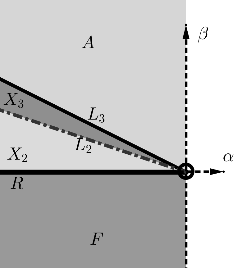
(c)

Figure 8:

In this section, we will introduce a way of thinking about quadrilaterals. This will help us prove Theorem  2.2.4.

Let $q$ be a quadrilateral. If $q$ is not rectangle, then we can choose an acute angle $\alpha$. For the two angles adjacent to $\alpha$, we pick the smaller one (or either one, if they are equal), and call it $\beta$, as shown in Figure  8a. If $q$ is a rectangle, then we let $\alpha=\frac{\pi}{2},\beta=\frac{\pi}{2}$. Then, every quadrilateral will be characterized by some point on the $\alpha$-$\beta$ plane, which consists of the left half plane $\left(\alpha<\frac{\pi}{2}\right)$ and the origin $\left(\alpha=\frac{\pi}{2},\beta=\frac{\pi}{2}\right)$, as shown in Figure  8b.

Note that a quadrilateral $q$ being close to the $\left(\frac{\pi}{2},\frac{\pi}{2}\right)$ point on the $\alpha$-$\beta$ plane does not tell anything about the “near-squareness” of the quadrilateral. For example, the point $\left(\frac{\pi}{2},\frac{\pi}{2}\right)$ represents the set of all rectangles (including those rectangles that are not “near-square” at all).

To prove Theorem  2.2.4, we chop the left half plane into 8 regions. We show that an $\frac{\pi}{107}$-near square $q$ has a periodic billiard path whose orbit type only depends on the region.

Region in $\alpha$-$\beta$ plane	in Figure  8c	orbit type	note
$\left(\frac{\pi}{2},\frac{\pi}{2}\right)$	origin	$0202$	Rectangles
$\alpha<\frac{\pi}{2},\beta<\frac{\pi}{2}$	$F$	$012012$	Section  3.2
$\alpha<\frac{\pi}{2},\beta=\frac{\pi}{2}$	$R$	$012021$	Section  3.3
$\alpha<\frac{\pi}{2},\alpha+2\beta>\frac{3}{2}\pi$	$A$	$01203213$	Section  3.4
$\alpha<\frac{\pi}{2},\alpha+3\beta<2\pi,\beta>\frac{\pi}{2}$	$X_{2}$	$0(13)^{2}013131310(31)^{2}03$	Section  3.5
$\alpha<\frac{\pi}{2},\alpha+3\beta>2\pi,\alpha+2\beta<\frac{3}{2}\pi$	$X_{3}$	$0(13)^{3}0(13)^{2}131(31)^{2}0(31)^{3}03$	Section  3.5
$\alpha<\frac{\pi}{2},\alpha+3\beta=2\pi$	$L_{2}$	$01313103$	Section  3.6
$\alpha<\frac{\pi}{2},\alpha+2\beta=\frac{3}{2}\pi$	$L_{3}$	$0131313103$	Section  3.6

3.2 Adjacent acute angles

In this section, we will prove the following:

Proposition 3.2.1.

If $q$ is $\frac{\varepsilon}{12}$-near square, and it has two adjacent acute angles, then $q$ has a periodic billiard path.

(a)

(b)

Figure 9:

We know that in every acute triangle, there’s a periodic billiard path, the Fagnano orbit. The orbit type is 012012. Now suppose a near square have two adjacent acute angles. Then we can complete this near square to an acute triangle, and then find the Fagnano orbit, as shown in Figure 9a. Then since the quadrilateral is near square, two of the altitudes have to be really flat, so the Fagnano orbit stays inside this near square. This gives a periodic billiard path of the near square, and let us give this orbit a name, orbit F.

Figure 10:

So, the central question now is how near square this path require. Let us consider Figure 9b. The critical condition is clearly that $\theta_{1}$ and $\theta_{2}$ as shown are smaller than $\frac{\pi}{2}$. We will need the following:

Lemma 3.2.2.

Let $ABCD$ be a quadrilateral as shown in Figure 10. Suppose $|\alpha_{i}-\frac{\pi}{4}|<\varepsilon$ for any $i$, and $\varepsilon<\frac{\pi}{12}$, then $|\beta_{j}-\frac{\pi}{4}|<3\cdot\varepsilon$ for any $j$.

The proof of this lemma is trigonometric (using Sine Rule) and some estimates using Mathematica. We will leave the proof of this lemma to the reader.

Proof of Prop  3.2.1.

Suppose quadrilateral $q$ is $\frac{\pi}{12}$ near square. Let $\theta_{1}$ and $\theta_{2}$ be the angle shown in figure  9b. By the above discussion, it suffice to show that $\theta_{i}<\frac{\pi}{2},i=1,2$. Depending on the choice of diagonal used in the parameterization, one of the two angles $\theta_{i}$ satisfies $\left|\theta_{i}-\frac{\pi}{4}\right|<\frac{\pi}{2}$. By the lemma, the other angle satisfies $\left|\theta_{j}-\frac{\pi}{4}\right|<\frac{\pi}{4}$ ∎

3.3 Acute angle adjacent to a right angle

Figure 11:

Proposition 3.3.1.

If $q$ is $\frac{\pi}{12}$-near square, and it has a right angle adjacent to an acute angle, then $q$ has a periodic billiard path.

The proof is the same as the proof of proposition  3.2.1. In this case, we need to show the angle $\theta$ of Figure  11 is acute.

3.4 Opposite acute angles

Figure 12: Orbit A

Here we are going to study a specific periodic billiard path with combinatorial orbit 01203213, whose unfolding is illustrated in Figure  12. The last two dotted quadrilateral is a translation of the first two quadrilateral. This orbit is clearly stable by Lemma  2.2.2, and the direction of translation (and thus the direction of the billiard path) is the same as the line connecting $b_{1}$ and $b_{1}^{\prime}$. If we let this be the $x$-axis, and let $y(b_{i})$ denote the $y$-coordinate of $b_{i}$ (similarly for $a_{i}$), then following the discussion after Figure  6, we would like to prove:

Proposition 3.4.1.

If the quadrilateral is $\frac{\pi}{30}$ near square, $\alpha,\theta$ in Figure  12 are acute, the other two angles are obtuse, then

$$\max_{j}y(b_{j})<\min_{i}y(a_{i})$$

and hence the quadrilateral has this periodic path.

Let us start with some observations.

Remark 3.4.2.

If our quadrilateral is $\frac{\pi}{12}$ near square, then $\max_{j}y(b_{j})=\max\{y(b_{1}),y(b_{3}),y(b_{6})\}$, and $\min_{i}y(a_{i})=\min\{y(a_{3}),y(a_{6}),y(a_{8})\}$

Proof.

Since our quadrilateral is convex, we know $y(a_{2})$ is definitely larger than the smaller one of $y(a_{1})$ and $y(a_{3})$, so we don’t need to consider the vertex $a_{2}$. Similarly we can eliminate vertices $a_{4},a_{7},b_{2},b_{5},b_{7}$.

Now suppose that our quadrilateral is $\dfrac{\pi}{12}$-near square, then we know $\angle b_{3}a_{5}a_{6}<\dfrac{2\pi}{3}$, and $\angle a_{3}a_{5}b_{3}<\dfrac{\pi}{3}$. So, we know $\angle a_{3}a_{5}a_{6}<\pi$. So again by convexity, $y(a_{5})$ is larger than the smaller one of $y(a_{3})$ and $y(a_{6})$. In the same fashion, we can eliminate vertices $a_{1},b_{4},b_{8}$. ∎

So, for Proposition  3.4.1, all that remains is to show:

$$\max\{y(b_{1}),y(b_{3}),y(b_{6})\}<\min\{y(a_{3}),y(a_{6}),y(a_{8})\}$$

Note that $y(a_{1}^{\prime})=y(a_{1}),y(b_{1}^{\prime})=y(b_{1})$. In this section, we use the word ‘angular slope’ to refer to the angle at which the line meets with the $x$-axis, i.e. ‘angular slope’ $=\tan^{-1}(m)$ with values in $\left(-\frac{\pi}{2},\frac{\pi}{2}\right)$, where $m$ is the gradient of the non-vertical line.

Proposition 3.4.3.

If the quadrilateral is $\dfrac{\pi}{4}$-near square, then $min(y(a_{6}),y(a_{8}))>max(y(b_{1}),y(b_{3}))$ if and only if both $\alpha$ and $\theta$ are acute.

Proof.

Let us restrict our attention to $b_{1},b_{3},a_{6},a_{8},b_{1}^{\prime},b_{3}^{\prime}$, as shown in Figure 13a, 13b, 13c, 13d. One can tell from Figure  12 that for the angles drawn in the Figures below, $\angle b_{1}b_{3}a_{6}=\angle a_{6}a_{8}b_{1}^{\prime}=2\alpha$, and $\angle b_{3}a_{6}a_{8}=\angle a_{8}b_{1}^{\prime}b_{3}^{\prime}=2\theta$. Note that $b_{1}b_{3},b_{3}a_{6},a_{6}a_{8},a_{8}b_{1}^{\prime},b_{1}^{\prime}b_{3}^{\prime}$ all have the same length, since they are the same diagonal of the same quadrilateral. Let us connect $b_{1}a_{6}$ and $a_{6}b_{1}^{\prime}$. Clearly, $\bigtriangleup b_{1}a_{6}b_{3}\cong\bigtriangleup b_{1}^{\prime}a_{6}a_{8}$ are the same isoceles triangle. So, $\angle b_{1}a_{6}b_{3}=\angle b_{1}^{\prime}a_{6}a_{8}$, and hence $\bigtriangleup b_{1}a_{6}b_{1}^{\prime}$ is an isosceles triangle with top angle $2\theta$ or $2\pi-2\theta$. So if $\theta$ is obtuse or right angled, then $y(a_{6})\leq 0=y(b_{1})$. Similarly, if $\alpha$ is obtuse or right angled, then observe from $\bigtriangleup b_{3}a_{8}b_{3}^{\prime}$ that $y(b_{3})\geq y(a_{8})$.

If both $\alpha$ and $\theta$ are acute (see Figure  13d), then $y(a_{6})>y(b_{1})$ and $y(b_{3})<y(a_{8})$. Hence, all that remains is to show $y(a_{6})>y(b_{3})$ and $y(a_{8})>y(b_{1})$. Using the isosceles triangles $\bigtriangleup b_{1}a_{6}b_{1}^{\prime}$ and $\bigtriangleup b_{1}b_{3}a_{6}$, we see that the slope of the line $b_{1}b_{3}$ is $\dfrac{\pi-2\theta}{2}-\dfrac{\pi-2\alpha}{2}=\alpha-\theta$. (Note: if $\alpha<\theta$, then $y(b_{3})<y(b_{1})$. This following argument is still valid after redrawing Figure  13d accordingly)

One can also see that the slopes of $b_{3}a_{6},a_{6}a_{8},a_{8}b_{1}^{\prime},b_{1}^{\prime}b_{3}^{\prime}$ are $\pi-\alpha-\theta,\theta-\alpha,\alpha+\theta-\pi,\alpha-\theta$ respectively.

So, to show $y(a_{6})>y(b_{1})$ and $y(a_{8})>y(b_{1}^{\prime})$ is equivalent to showing the slope of $b_{3}a_{6}$ is bigger than zero and the slope of $a_{8}b_{1}^{\prime}$ is less than zero (i.e. $0<\pi-\alpha-\theta<\frac{\pi}{2}$ and $0>\alpha+\theta-\pi>-\frac{\pi}{2}$). Note that $\alpha,\theta<\frac{\pi}{2}$ implies $\pi-\alpha-\theta>0$. Furthermore, if the quadrilateral is $\frac{\pi}{4}$-near square, then $\alpha,\theta>\frac{\pi}{4}$, which implies $\pi-\alpha-\theta<\frac{\pi}{2}$. This completes the proof. ∎

Proposition 3.4.4.

When the quadrilateral is $\dfrac{\pi}{12}$-near square, then $y(a_{3})>\max(y(b_{1}),y(b_{3}))$, and $\min(y(a_{6}),y(a_{8}))>y(b_{6})$.

Proof.

We know from Proposition  3.4.3 that the slope of $b_{1}b_{3}$ is $\alpha-\theta$, which is between $\dfrac{\pi}{6}$ and $-\dfrac{\pi}{6}$ when the quadrilateral is $\dfrac{\pi}{12}$-near square. As $\angle a_{3}b_{1}b_{3}$ is between $\dfrac{\pi}{6}$ and $\dfrac{\pi}{3}$, we see that the slope of $b_{1}a_{3}$ is between $\dfrac{\pi}{2}$ and $0$. So it has positive slope, and $y(a_{3})>y(b_{1})$. By basically the same argument, we can show that $y(a_{3})>y(b_{3}),y(a_{6})>y(b_{6}),y(a_{8})>y(b_{6})$. ∎

(a)

(b)

(c)

(d)

Figure 13: (a)$\alpha<\frac{\pi}{2}$, $\theta>\frac{\pi}{2}$, (b) $\alpha>\frac{\pi}{2}$, $\theta<\frac{\pi}{2}$ (c) $\alpha>\frac{\pi}{2}$, $\theta>\frac{\pi}{2}$ (d) $\alpha<\frac{\pi}{2}$, $\theta<\frac{\pi}{2}$

Lemma 3.4.5.

In an $\epsilon$-near square, if one edge has length 1, then the length of the adjacent edge is between $\tan\left(\dfrac{\pi}{4}-\epsilon\right)\cos\left(2\epsilon\right)$ and $\dfrac{\tan\left(\frac{\pi}{4}+\epsilon\right)}{\cos(2\epsilon)}$.

Proof.

WLOG, for Figure  10, let $|AC|=1$. Then by sine rule:

$$\dfrac{BC}{AC}=\dfrac{BC}{1}=\dfrac{\sin\alpha_{1}}{\sin\alpha_{2}},\hskip 14.22636pt\dfrac{AD}{AC}=\dfrac{AD}{1}=\dfrac{\sin\beta_{1}}{\sin\beta_{2}}=\dfrac{\sin\alpha_{4}}{\sin(\alpha_{2}+\alpha_{4})}\dfrac{\sin(\alpha_{1}+\alpha_{3})}{\sin\alpha_{3}}$$

We will leave the rest of the estimation to the reader. ∎

Proposition 3.4.6.

When the quadrilateral is $\dfrac{\pi}{30}$-near square, $\alpha$ and $\theta$ are acute, and the other two angles are obtuse, then $y(a_{3})>y(b_{6})$.

Figure 14:

Proof.

Clearly the line $a_{3}a_{3}^{\prime}$ is parallel to the $x$-axis. Then it clearly follows that $y(a_{3})>y(b_{6})$ if and only if $\angle a_{3}b_{6}a_{3}^{\prime}<\pi$ (See figure  12)

Let us first look at $\angle a_{6}b_{6}a_{3}$ by breaking it down into three angles, $\tau_{1},\tau_{2},\tau_{3},$ as shown in Figure  14. Suppose our quadrilateral is $\frac{\pi}{30}$-near square, then (See figure  12) $\theta>\frac{\pi}{2}-2\frac{\pi}{30}=\frac{13\pi}{30}$, so $\angle a_{5}a_{6}b_{6}=2\theta>\frac{13\pi}{15}$. As $\bigtriangleup a_{5}a_{6}b_{6}$ is an isosceles triangle, we see that $\tau_{1}<\frac{\pi}{15}$. (also, since $\theta<\frac{\pi}{2}$, so $\tau_{1}>0$)

Let $\angle a_{6}b_{6}a_{8}=\beta$. Then $\angle a_{4}a_{5}a_{6}=2\beta$ as shown, and $\angle a_{4}a_{5}b_{6}=2\beta-\tau_{1}>2\beta-\frac{\pi}{15}$. If $\angle a_{4}a_{5}b_{6}\geq\pi$, then $\tau_{2}\leq 0$ (i.e. in the figure above, $\tau_{1}$ and $\tau_{3}$ overlap). So $\tau_{1}+\tau_{2}\leq\tau_{1}<\frac{\pi}{15}$.

Note that $a_{5}b_{6}=2\cos(\angle a_{6}b_{6}a_{5})\cdot a_{6}b_{6}>2\cos\frac{\pi}{15}*a_{6}b_{6}>a_{6}b_{6}=a_{4}a_{5}$. So, if $\angle a_{4}a_{5}b_{6}<\pi$, then $a_{5}b_{6}>a_{4}a_{5}$ implies $\tau_{2}<\angle a_{5}a_{4}b_{6},$ hence $\tau_{2}<\dfrac{\angle a_{5}a_{4}b_{6}+\tau_{2}}{2}=\dfrac{\pi-\angle a_{4}a_{5}b_{6}}{2}<\dfrac{\pi-(2\beta-\frac{\pi}{15})}{2}=\frac{8\pi}{15}-\beta$.

WLOG, let the length $a_{4}a_{5}=a_{5}a_{6}=a_{6}b_{6}=1$, then we know that $a_{5}b_{6}>2\cos\frac{\pi}{15}$. Note that $\beta\in(\frac{\pi}{2},\frac{17}{30}\pi),\tau_{1}\in(0,\frac{\pi}{15})$, so $\angle a_{4}a_{5}b_{6}=2\beta-\tau_{1}\in(\frac{14}{15}\pi,\frac{17}{15}\pi)$ (and hence $\cos(\angle a_{4}a_{5}b_{6})<0$).

Then we can see that the length $a_{4}b_{6}>\sqrt{1^{2}+(2\cos\frac{\pi}{15})^{2}-2\cdot 1\cdot 2\cos\frac{\pi}{15}\cdot\cos(\frac{17}{15}\pi)}\approx 2.89852$. We also know by Lemma 3.4.5 that the length $a_{3}a_{4}<\dfrac{\tan(\frac{\pi}{4}+\frac{\pi}{30})}{\cos\frac{\pi}{15}}\approx 1.26249$. Note that $\sin\tau_{3}\leq\dfrac{a_{3}a_{4}}{a_{4}b_{6}}<\frac{1.26249}{2.89852}\approx 0.43556$. So $\tau_{3}<p=0.45066$.

So now if $2\beta-\frac{\pi}{15}\geq\pi$, then $\angle a_{4}a_{5}b_{6}\geq\pi$, and so $\tau_{1}+\tau_{2}+\tau_{3}<\frac{\pi}{15}+p$. If $2\beta-\frac{\pi}{15}<\pi$, then $\angle a_{6}b_{6}a_{3}=\tau_{1}+\tau_{2}+\tau_{3}<(\frac{\pi}{15})+(\frac{8\pi}{15}-\beta)+p=\frac{3\pi}{5}-\beta+p$. But the latter one is clearly looser in this case, so we use the latter inequality. Similarly, one can also show that $\angle a^{\prime}_{3}b_{6}a_{8}<\frac{3\pi}{5}-\beta+p$. So $\angle a_{3}b_{6}a_{3}^{\prime}<2(\frac{3\pi}{5}-\beta+p)+\beta<2p+\frac{6\pi}{5}-\beta<2p+\frac{6\pi}{5}-\frac{\pi}{2}\approx 3.10043<\pi$. Here the second to last inequality follows because $\beta$ is supposed to be obtuse. This proves the proposition.

∎

For a summary, a quadrilateral which is $\frac{\pi}{30}$-near square has orbit A if it has two opposite acute angles and two opposite obtuse angles (i.e. it is represented in the region $A$ in Figure  8c).

3.5 The $X$ family orbits

The $X$ family orbits is an infinite family of orbits, starting from $X_{2}$. Let us first study $X_{2}$, and then study the general pattern of the $X$ family orbits.

Figure 15: Unfolding of $X_{2}$ orbit

Up to a relabeling of the edges, $X_{2}$ has the orbit type 01313013131310313103. This is clearly stable by Lemma  2.2.2. An unfolding would look like Figure  15. The first obvious feature of $X_{2}$ is that the unfolding is symmetric about the line $\ell_{9}$. Note that the motion from $\ell_{1}$ to $\ell_{1}^{\prime}$ is a translation. So, if we build a coordinate frame using $b_{1}b_{1}^{\prime}$ as the $x$-axis and let $\ell_{1}$ as the $y$-axis, then $\ell_{1},\ell_{9},$ and $\ell_{1}^{\prime}$ are vertical.

Now to find the condition for this orbit to exist, we must find the condition when all top vertices are above all bottom vertices. i.e. in Figure  15, we want to show:

$$\max_{j}y(b_{j})<\min_{i}y(a_{i})$$

Since everything is symmetric about $\ell_{9}$, we only need to consider the left half part of the unfolding. In the following proof, we shall use $v|\ell|w$ to denote the fact that the objects $v$ and $w$ are symmetric about the line $\ell$. Furthermore, we shall use $s(\ell)$ to denote the ‘angular slope’ of the line $\ell$ (‘angular slope’ $=\tan^{-1}(m)$ with values in $\left(-\frac{\pi}{2},\frac{\pi}{2}\right)$, where $m=$ gradient of $\ell$). In addition, we use the notation $\min y(a_{1},a_{2},a_{3})$ to denote the minimum of $\{y(a_{1}),y(a_{2}),y(a_{3})\}$, and similar notation for the maximum.

Proposition 3.5.1.

Suppose the quadrilateral is $\dfrac{\pi}{16}$-near square, then in Figure  15, TFAE:

1. $\min y(a_{3},a_{6})>\max(b_{1},b_{8})$

2. $s(\ell_{3})<0,s(\ell_{4})>0$ and $s(h_{1})>0$.

3. $\alpha<\frac{\pi}{2},\beta>\frac{\pi}{2},3\beta+\alpha<2\pi$

Proof.

$(1)\Rightarrow(2)$: Since $y(a_{6})>y(b_{1})$ and $b_{1}|\ell_{3}|a_{6}$, we see that $s(\ell_{3})<0$. Since $y(a_{3})>y(b_{8})$ and $a_{3}|\ell_{4}|b_{8}$, we see that $s(\ell_{4})>0$. Since $y(a_{3})>y(b_{1})$, we see that $s(h_{1})>0$.

$(2)\Rightarrow(3)$: One can verify that $s(h_{1})=\frac{\pi}{2}-\alpha,s(\ell_{3})\equiv s(h_{1})+2\beta+\alpha=\frac{\pi}{2}+2\beta(\text{mod }\pi)$, and $s(\ell_{4})\equiv s(\ell_{3})+\alpha+\beta=\frac{\pi}{2}+3\beta+\alpha(\text{mod }\pi)$. Assume for contradiction that $\frac{3\pi}{8}<\beta\leq\frac{\pi}{2}$ (the first inequality is due to the near-squareness). Then $\pi+\frac{1}{4}\pi<2\beta+\frac{\pi}{2}\leq\pi+\frac{\pi}{2}$. So, after taking modulo $\pi$, we get $s(\ell_{3})>0$ (which contradicts (2)). Similarly, we can argue that $\alpha<\frac{\pi}{2}$ and $3\beta+\alpha<2\pi$.

$(3)\Rightarrow(2)\&(1)$: The near square condition also gives us $\alpha>\dfrac{3\pi}{8},\beta<\dfrac{5\pi}{8}$. So, using the conditions in (3), we can get the inequalities in $(2)$, $\ell_{2},h_{2}$ having negative slope and $\ell_{5},\ell_{6},\ell_{7},\ell_{8}$ having positive slope. Now the slope of $h_{1},h_{2}$ makes sure that $y(a_{3})>y(b_{1}),y(a_{6})>y(b_{8})$. And as $b_{1}|\ell_{3}|a_{6},a_{3}|\ell_{4}|b_{8}$, we have $y(a_{6})>y(b_{1})$, and $y(a_{3})>y(b_{8})$. This completes our proof. ∎

Remark 3.5.2.

If the condition for Prop  3.5.1 is satisfied, and the angle $\gamma$ is obtuse, then
$\displaystyle\max_{j}y(b_{j})=\max y(b_{1},b_{4},b_{5},b_{8}),\min_{i}y(a_{i})=\min y(a_{3},a_{6},a_{11})$

Proof.

If $\gamma$ is obtuse, then immediately we know $y(a_{2})>y(a_{1}),y(a_{10})>y(a_{11}),$ so vertices $a_{2},a_{10}$ are eliminated.

Now as $a_{3}|\ell_{3}|a_{5},a_{4}|\ell_{4}|a_{6},$ by the slope of $\ell_{3}$ and $\ell_{4}$ we must have $y(a_{5})>y(a_{3}),y(a_{4})>y(a_{6})$. So we don’t need to consider vertices $a_{4},a_{5}$. We also have $b_{8}|\ell_{7}|b_{10},b_{9}|\ell_{8}|b_{11},$ so similarly we eliminate vertices $b_{10},b_{11}$. We also know that $\angle b_{8}b_{9}b_{10}=2\alpha<2\pi$, so $y(b_{9})<max(y(b_{8}),y(b_{10}))$, and we eliminate $b_{9}$.

As $a_{7}|\ell_{6}|a_{9},a_{8}|\ell_{7}|a_{10},a_{9}|\ell_{8}|a_{11},$ we see that $y(a_{7})>y(a_{9})>y(a_{11}),y(a_{8})>y(a_{10})>y(a_{11})$, so we eliminate $a_{7},a_{8},a_{9}$. Similarly, as $b_{2}|\ell_{2}|b_{4},b_{3}|\ell_{3}|b_{5},b_{4}|\ell_{4}|b_{6},b_{5}|\ell_{5}|b_{7},$ so $y(b_{2})<y(b_{4}),y(b_{3})<y(b_{5}),y(b_{6})<y(b_{4}),y(b_{7})<y(b_{5})$. So we eliminate $b_{2},b_{3},b_{6},b_{7}$.

Finally, one can use the $\frac{\pi}{12}$ near squareness to estimate and get the result $y(a_{1})>y(a_{3})$, and so we can eliminate $a_{1}$. ∎

Proposition 3.5.3.

If the condition for Prop  3.5.1 is satisfied, and the quadrilateral is $\dfrac{\pi}{56}$-near square and the angle $\gamma$ is obtuse, then $\displaystyle\max y(b_{1},b_{4},b_{5},b_{8})=\max y(b_{1},b_{8}),\min y(a_{3},a_{6},a_{11})=\min y(a_{3},a_{6})$

Proof.

In this proof, we will show that $y(a_{11})>y(a_{6}),y(b_{4})<y(b_{1}),y(b_{5})<y(b_{1})$.

Suppose the length $b_{10}b_{11}=1$. Then by lemma  3.4.5 we know:

$$y(a_{11})\geq y(b_{11})+\tan(\dfrac{\pi}{4}-\dfrac{\pi}{56})\cos\dfrac{\pi}{28}\approx 0.8880356$$

We can also calculate that:

$$y(a_{6})=y(b_{11})+\cos\alpha-\cos(\alpha+2\beta)+\cos(3\alpha+2\beta)-\cos(3\alpha+4\beta).$$

Note that $\frac{\pi}{2}-2\varepsilon<\alpha<\frac{\pi}{2},\beta\geq\frac{\pi}{2}$. So, we have (by letting $\varepsilon=\frac{\pi}{56}$)

$$y(a_{6}) \leq y(b_{11})+\cos\left(\frac{\pi}{2}-2\varepsilon\right)-\cos\left(\frac{\pi}{2}-2\varepsilon+2\cdot\frac{\pi}{2}\right)+\cos\left(3\left(\frac{\pi}{2}-2\varepsilon\right)+2\cdot\frac{\pi}{2}\right)$$

$$-\cos\left(3\left(\frac{\pi}{2}-2\varepsilon\right)+4\cdot\frac{\pi}{2}\right)\approx 0.884487$$

A calculation shows that $y(a_{11})>y(a_{6})$.

We have shown that $a_{11}$ is the lowest of $a_{7},a_{8},a_{9}$ and $a_{10}$. If we draw a line through $a_{6}$ perpendicular to $\ell_{9}$, then $a_{7},a_{8},a_{9},a_{10},a_{11}$ would all lie above this line. So for the same reason, if we draw a line through $b_{1}$ perpendicular to $\ell_{5}$, then $b_{2},b_{3},b_{4},b_{5},b_{6}$ would all lie below this line. As $\ell_{5}$ has positive slope, clearly this perpendicular line has negative slope. So we see that $y(b_{4})<y(b_{1})$ and $y(b_{5})<y(b_{1})$. ∎

By combining the Propositions and Remark, we conclude that a quadrilateral has orbit $X_{2}$ if the following conditions are satisfied:

1. the quadrilateral is $\dfrac{\pi}{56}$-near square;

2. the quadrilateral has one acute angle $\alpha$, and two obtuse angle adjacent to $\alpha$;

3. one of the obtuse angle $\beta$ adjacent to $\alpha$ satisfies the inequalities $2\beta>\pi$ and $\alpha+3\beta<2\pi$.

Note that the region $X_{2}$ in Figure  8c does satisfy these properties, and hence have this periodic billiard path. (It is also worth mentioning that we do not need $\beta$ to be the smaller of the two angles adjacent to $\alpha$.)

Figure 16: Unfolding of $X_{3}$ orbit

Figure 17: Half unfolding of $X_{4}$ orbit

Now we are ready to explore other orbits in the $X$ family. In general, the orbit $X_{n}$ will have orbit type $0(13)^{n}0(13)^{n-1}131(31)^{n-1}0(31)^{n}03$, and some unfolding are in Figure  16,  17. The conditions for these orbits to work is similar to $X_{2}$, and the proof is basically identical. For any integer n, a quadrilateral has orbit $X_{n}$ if the following conditions are satisfied:

1. the quadrilateral is $\varepsilon_{n}$-near square;

2. the quadrilateral has one acute angle $\alpha$, and two obtuse angle adjacent to $\alpha$;

3. one of the obtuse angle $\beta$ adjacent to $\alpha$ satisfies the inequalities $(n-2)\alpha+n\beta>(n-1)\pi$ and $(n-1)\alpha+(n+1)\beta<n\pi$.

Here $\varepsilon_{n}$ is a decreasing sequence with limit $0$ as $n$ goes to $\infty$. $\varepsilon_{n}$ the real root nearest to $0$ of the following equation: Let $x_{n}=\dfrac{\pi}{2}-2\epsilon_{n},y_{n}=\dfrac{n-1}{n}\pi-\dfrac{n-2}{n}x_{n},y_{n}^{\prime}=\frac{\pi}{2}$, then:

$$\tan\left(\dfrac{\pi}{4}-\varepsilon_{n}\right)\cos(2\varepsilon_{n})=\sum_{i=1}^{n}\cos\left[(2i-1)x_{n}+(2i-2)y_{n}\right]-\sum_{i=1}^{n}\cos\left[(2i-1)x_{n}+(2i)y_{n}^{\prime}\right]$$ (3.5.1)

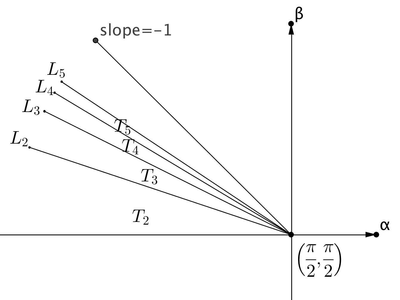
Figure 18: Coordinate Space

Condition 2 and 3 implies that $X_{n}$ covers the region $T_{n}$ in the $\alpha$-$\beta$ plane of Figure  18 (as long as the quadrilateral is sufficiently near square). The gradient of $L_{n}$ is $-\frac{n-1}{n+1}$, which goes to $-1$ as $n$ goes to $\infty$. Note that gradient of $L_{3}$ is $-1/2$, and the orbit $A$ in Section 3.4 covers the region above the line $L_{3}$.

In short, if the quadrilateral is described in region $T_{3}$ [$T_{2}$, respectively] and is $\varepsilon_{3}$-near square [$\varepsilon_{2}$], then it has the orbit $X_{3}$ [$X_{2}$].

One can calculate that $\varepsilon_{3}$ is slightly larger than $\frac{\pi}{107}$, and so the near-squareness condition for $X_{3}$ is more strict than that of $X_{2}$. The only thing left is the lines $L_{2},L_{3}$, which will be solved by the Y family.

3.6 The $Y$ family orbits

(a)

(b)

Figure 19: Unfolding for (a)$Y_{2}$, (b) $Y_{3}$

The $Y$ family orbits is a family of unstable orbit which covers exactly $L_{n}$ in Figure  18. Some unfoldings are shown in Figure  19a,  19b with the parameter angle $\alpha$ and $\beta$ marked.

For example, let us look at $X_{2}$ in Figure  15. If the quadrilateral lies on $L_{2}$ in the $\alpha$-$\beta$ parameter plane, then the line $\ell_{4}$ is vertical. So, if we reflect the first four square in the unfolding of Figure 15, we would get the unfolding in Figure  19a, which we call $Y_{2}$. The whole $Y$ family arises this way, and the near-square condition (for this orbit to work) is looser than that for the $X$ family (since there are less vertices to consider compared to $X$ orbits).

To sum up, if a quadrilateral is $\varepsilon_{n}$-near square and lies on the line $L_{n}$ in the $\alpha-\beta$ parameter plane, then it has orbit $Y_{n}$.

3.7 Summary

So now let us put the whole proof together. Any quadrilateral $q$, suppose it is $\dfrac{\pi}{107}$-near square.

1. If it is a rectangle, then it has a periodic path where the ball bounces between two parallel lines.

2. If $q$ is not a rectangle, then it has at least one acute angle, call it $\alpha$. If one of the angle adjacent to $\alpha$ is acute, then $q$ has orbit $F$. If one of the angle adjacent to $\alpha$ is $90^{\circ}$, then $q$ has orbit $R$.

3. Suppose that both angles adjacent to $\alpha$ are obtuse, and let us call the smaller one $\beta$, the larger one $\gamma$. If the angle opposing $\alpha$ is acute, then $q$ has orbit $A$.

4. Assume that the angle opposing $\alpha$ is larger than or equal to $\dfrac{\pi}{2}$ and call it $\theta$. Then we know $\alpha+2\beta+\dfrac{\pi}{2}\leq\alpha+\beta+\gamma+\theta=2\pi$, so $\alpha+2\beta\leq\dfrac{3\pi}{2}$. So in the $\alpha$-$\beta$ plane, the only region left is $T_{2},T_{3},L_{2},L_{3}$. And these regions are covered by orbit $X_{2},X_{3},Y_{2},Y_{3}$.

This completes our proof for Theorem 2.2.4.

4 Proof of Theorem  2.2.5

The proof is pretty much identical to that of Theorem  2.2.4. All these orbits still works for rectangles. Fix a rectangle $K$. For any quadrilateral $q$, suppose it is sufficiently near $K$. If $q$ is a rectangle, then clearly it has a periodic path. If it has two adjacent acute angle, then it has orbit $F$. If it has one acute angle adjacent to a right angle, then it has orbit $R$. If it has two acute angle opposing each other, then it will have orbit $A$.

Suppose it has at least one acute angle $\alpha$, two adjacent obtuse angle, and the opposite angle to $\alpha$ is not acute. Let $\beta$ be the smallest of the obtuse angles adjacent to $\alpha$. Again, we have the inequality $\alpha+2\beta<\dfrac{3\pi}{2}$, and the orbits $X_{2},X_{3},Y_{2},Y_{3}$ covers these remaining regions in the $\alpha$-$\beta$ parameter plane.

The critical question is how near to the fixed rectangle $K$ do we need? Unfortunately this is not easy to answer, as this condition depends on which fixed rectangle $K$ we choose. The “flatter” the rectangle $K$ is, the stricter the condition will need to be.
Acknowledgement. We would like to thank Prof. W Patrick Hooper for his mentoring and support throughout our research, and for providing us with ‘McBilliards II’, a Java program that searches for periodic billiard paths. We drew lots of observation and inspiration from this Java program. ‘McBilliards II’ is available online at http://wphooper.com/visual/mcb2/.

References

- [1] M. Boshernitzan, G. Galperin and T. Krüger and S. Troubetzkoy, Periodic Billiard Orbits Are Dense in Rational Polygons, Transactions of the American Mathematical Society, 350(9) (1998), 3523–3535.
- [2] W. P. Hooper and R. E. Schwartz, Billiards in Nearly Isosceles Triangles, Journal of Modern Dynamics, 3(2) (2009), 159–231.
- [3] H. Masur and S. Tabachnikov, Rational billiards and flat structures, Handbook Dynamical Systems, 1A (2002), 1015–1089.
- [4] R. E. Schwartz, Obtuse Triangular Billiards I: Near the (2,3,6) Triangle, Journal of Experimental Mathematics, 15(2) (2006), 161–182.
- [5] R. E. Schwartz, Obtuse Triangular Billiards II: 100 Degrees Worth of Periodic Trajectories, Journal of Experimental Mathematics, 18(2) (2008), 137-171.
- [6] S. Tabachnikov, Billiards, Panoramas et Synthèses. 1. Paris: Société Mathématique de France. vi, 142 p., 1995.