Sequential Bayesian Learning for Merton’s Jump Model with Stochastic Volatility

Abstract

Jump stochastic volatility models are central to financial econometrics for volatility forecasting, portfolio risk management, and derivatives pricing. Markov Chain Monte Carlo (MCMC) algorithms are computationally unfeasible for the sequential learning of volatility state variables and parameters, whereby the investor must update all posterior and predictive densities as new information arrives. We develop a particle filtering and learning algorithm to sample posterior distribution in Merton’s jump stochastic volatility. This allows to filter spot volatilities and jump times, together with sequentially updating (learning) of jump and volatility parameters. We illustrate our methodology on Google’s stock return. We conclude with directions for future research.

Keywords: Bayes, Markov Chain Monte Carlo, Particle Filtering, Particle learning, Merton’s Model, Jumps, Stochastic Volatility, Credit Risk, Value-at-Risk.

1 Introduction

Jump stochastic volatility models are central to many questions in finance such as pricing, or debt-and-credit risk assessment. Merton (1976); Duffie et al. (2000) provide theoretical treatments of derivatives pricing and Merton (1974); Korteweg and Polson (2008) provide applications to debt and credit risk assessment. Most theoretical treatments in the literature assume the availability of efficient estimates of volatility, jumps and parameters. Efficient estimates of the current volatility state and jump parameters are available from Markov Chain Monte Carlo (MCMC) algorithms, see Johannes and Polson (2010); Jacquier et al. (2004). A number of authors have analyzed jump diffusion models by MCMC, see Eraker et al. (2003); Li et al. (2008); Fulop et al. (2012). One caveat is that MCMC algorithms are computationally demanding, and are not feasible for sequential learning. Essentially, MCMC algorithm needs to be run every time new information is available.

Particle filtering (PF) and learning (PL) algorithms, on the other hand, efficiently incorporate new information into the parameter learning process. Early PL algorithms where plagued by degeneracy problem which hampered their performance. Particle learning (Carvalho et al. (2010); Warty et al. (2016)) algorithms deliver posterior and predictive densities of parameters and latent variable as new information arrives. Sequential parameter learning is obtained by tracking a state vector of conditional sufficient statistics.

An important goal of an investor, for example, is to characterize the density of current and future returns to draw inference on the riskiness of a portfolio, probability of shortfall, or value-at-risk. The distribution of future volatility is an input in the computation of derivative prices or their hedge ratios. We provide a versatile model of access returns that combines Merton’s pure jump formulation with stochastic volatility. Within this model, the investor needs to learn about the state variables, namely, volatility, jump times and jump sizes, and the model parameters from the observed returns. PL methods are particularly well-suited for empirical finance applications for several reasons.

1. They are designed to be sequential, updating the relevant posterior distribution as new information (data) is obtained, with minimal computing resources. Bayesian inference tools directly apply to these PF algorithms as they produce posterior or predictive densities relevant to the models used.

2. Akin to MCMC algorithms, particle filtering and learning can be extended to simultaneously estimate both structural parameters and latent variables. For example, one can separate out the effects of jumps and stochastic volatility in equity returns.

3. As conditional simulation methods, they avoid optimization. From a practical perspective, PF and PL methods are therefore extremely fast in terms of computing time. This has many advantages, particularly for higher-dimensional multivariate models.

One can also included option price information into the inference problem, see for example Polson and Stroud (2003); Johannes and Polson (2009); Yun (2014). Whilst we only account for stochastic jumps, it is easy to add deterministic jump components to account for example, for earnings announcement effects, see Dubinsky and Johannes (2005).

The rest of the paper is as follows. Section 2 provides a review of particle filtering methods. Section 3 provides the main contribution of our paper and an algorithm for sequential filtering states and performing parameter learning for Merton Jump model together with stochastic volatility (Jacquier et al. (1995, 2004)). Section 4 provide a application to Google’s stock return. Finally, Section 5 concludes with directions for future research.

2 Particle Filtering for Merton’s Jump Model

Merton’s Jump Stochastic volatility model has a discrete time version for log-returns, $y_{t}$, with jump times, $J_{t}$, jump sizes, $Z_{t}$, and spot stochastic volatility, $V_{t}$, given by the dynamics

$$y_{t} \equiv\log\left(S_{t}/S_{t-1}\right)=\mu+V_{t}\varepsilon_{t}+J_{t}Z_{t}$$

$$V_{t+1} =\alpha_{v}+\beta_{v}V_{t}+\sigma_{v}\sqrt{V_{t}}\varepsilon_{t}^{v}$$

where $\mathbb{P}\left(J_{t}=1\right)=\lambda$. The errors $(\varepsilon_{t},\varepsilon_{t}^{v})$ are possibly correlated bivariate normals.

The investor must obtain optimal filters for $(V_{t},J_{t},Z_{t})$, and learn the posterior densities of the parameters $(\mu,\alpha_{v},\beta_{v},\sigma_{v}^{2},\lambda)$. These estimates will be conditional on the information available at each time.

2.1 Pure Jump Merton model

Let $S_{t}$ denote a stock or asset price. We have historical log-returns $y^{t}=(y_{1},\ldots,y_{t})$ defined by $y_{t}=\log(S_{t}/S_{t-1})$. Log-returns have a jump component as per

$$y_{t}=\mu+\sigma\varepsilon_{t}+J_{t}Z_{t},$$

with the probability of jump $\mathbb{P}\left[J_{t}=1\right]=\lambda\in\left(0,1\right)$ and $Z_{t}$ is the jump size. The Merton model involves the following hierarchical conditional distributions:

$$(\mu,\sigma^{2}) \sim NIG(m,n,a,b),$$

$$\lambda \sim Beta(\alpha,\beta),$$

$$J_{t}|\Theta \sim Ber(\lambda),$$

$$Z_{t}|\Theta,J_{t} \sim\mathcal{N}(\mu_{J},\sigma_{J}^{2}\sigma^{2}),$$

$$Y_{t}|\Theta,J_{t},Z_{t} \sim\mathcal{N}(\mu+J_{t}Z_{t},\sigma^{2}),$$

where $NIG$ denotes the standard conditionally conjugate Normal-Inverse-Gamma distribution. The parameters $\mu_{J},\sigma_{J}^{2}$ are fixed to guarantee identification. The goal of underlying dynamics is to provide sequential learning plot for states $(J_{t},Z_{t})$ and the unknown parameters $(\mu,\sigma^{2},\mu_{J},\sigma^{2}_{J},\lambda)$.

To construct a particle filtering and learning algorithm that samples from the set of Bayesian joint posterior distributions $p(J_{t},Z_{t},\theta|y^{t})$, for $1\leq t\leq T$. We track a particle vector that tracks the hidden states $\{J_{t},Z_{t}\}^{(i)}$ and the conditional sufficient statistics $\{s_{t}\}^{(i)}$ for any static parameters that need to be learned. Then attach them in one vector $\{J_{t},Z_{t},s_{t}\}^{(i)}$ for $1\leq i\leq N$.

Our Particle learning algorithm has four steps:

1. Determine the conditional sufficient statistics $s_{t}$ for the parameters $\theta=(\mu,\sigma^{2},\lambda)$. We write $p(\theta|s_{t})$ where $s_{t}=(m_{t},n_{t},a_{t},b_{t},\alpha_{t},\beta_{t})$ with the following distributional assumptions

   $$p(\mu,\sigma^{2}|J_{1:t},Z_{1:t},y_{1:t})\equiv p(\mu,\sigma^{2}|s_{t})\sim NIG\left(m_{t},n_{t},a_{t},b_{t}\right)\;\;{\rm and}\;\;(\lambda|s_{t})\sim Beta(\alpha_{t},\beta_{t}).$$

   This leads to a current posterior distribution, $p(\mu,\sigma^{2},\lambda|s_{t})$ that is proportional to

   $$(\sigma^{2})^{-a_{t}-3/2}\exp\left(-\frac{n_{t}(\mu-m_{t})^{2}+2b_{t}}{2\sigma^{2}}\right)\lambda^{\alpha_{t}-1}(1-\lambda)^{\beta_{t}-1}.$$

   The conditional likelihood $p(Y_{t+1},J_{t+1},Z_{t+1}|\mu,\sigma^{2},\lambda)$ proportional to

   $$\lambda^{J_{t+1}}(1-\lambda)^{1-J_{t+1}}\times(\sigma_{J}^{2}\sigma^{2})^{-1/2}\exp\left(-\frac{(Z_{t+1}-\mu_{J})^{2}}{2\sigma_{J}^{2}\sigma^{2}}\right)\times$$

   $$(\sigma^{2})^{-1/2}\exp\left(-\frac{(Y_{t+1}-\mu-J_{t+1}Z_{t+1})^{2}}{2\sigma^{2}}\right).$$

   Combining these two terms, leads to an updated conditional posterior, $p(\mu,\sigma^{2},\lambda|s_{t+1})$ with is again a $NIG\times Beta$ distribution with updated hyperparameters

   $$m_{t+1}=\frac{n_{t}m_{t}+R_{t+1}}{n_{t}+1},n_{t+1}=n_{t}+1,$$

   $$a_{t+1}=a_{t}+1\;{\rm and}\;b_{t+1}=b_{t}+\frac{n_{t}(R_{t+1}-m_{t})^{2}}{2(n_{t}+1)}+\frac{(Z_{t+1}-\mu_{J})^{2}}{2\sigma_{J}^{2}}$$

   where $R_{t}=Y_{t}-J_{t}Z_{t}$, and $\alpha_{t+1}=\alpha_{t}+J_{t+1}$ and $\beta_{t+1}=\beta_{t}+1-J_{t+1}$.

2. Calculate the marginal predictive distribution, denoted by $p(y_{t+1}\mid J_{t},Z_{t},s_{t})$ of the next asset return $y_{t+1}$ given the states $J_{t+1},Z_{t+1}$. This a mixture distribution of the form

   $$\int\sum_{J_{t+1}}p(y_{t+1}|J_{t+1},Z_{t+1},\mu,\sigma^{2})p(Z_{t+1}|\lambda)p(J_{t+1}|\lambda)p(\mu,\sigma^{2},\lambda|s_{t})d\mu d\sigma^{2}d\lambda$$

   We marginalise out the states $Z_{t+1},J_{t+1}$ and the parameters $\mu,\sigma^{2},\lambda$, as follows. First, marginalizing $Z_{t+1}$ and $\lambda$, we obtain

   $$p(\mu,\sigma,J_{t+1},y_{t+1}|s_{t})\propto\gamma_{t+1}^{1/2}B(\alpha_{t+1},\beta_{t+1})\times NIG(m_{t+1},n_{t+1},a_{t+1},b_{t+1})$$

   where with hyperparameter updates are given by

   $$\gamma_{t+1}=\frac{1}{1+J_{t+1}\sigma_{J}^{2}},$$

   $$m_{t+1}=\frac{n_{t}m_{t}+\gamma_{t+1}Q_{t+1}}{n_{t}+\gamma_{t+1}}\;{\rm where}\;Q_{t+1}=y_{t+1}-J_{t+1}\mu_{J},$$

   $$n_{t+1}=n_{t}+\gamma_{t+1},$$

   $$a_{t+1}=a_{t}+\frac{1}{2},$$

   $$b_{t+1}=b_{t}+\frac{n_{t}\gamma_{t+1}(Q_{t+1}-m_{t})^{2}}{2(n_{t}+\gamma_{t+1})}.$$

   Therefore, we have a marginal joint posterior

   $$p(y_{t+1},J_{t+1}|s_{t})\propto B(\alpha_{t+1},\beta_{t+1})\gamma_{t+1}^{1/2}n_{t+1}^{-1/2}b_{t+1}^{-a_{t+1}}.$$

   Finally, marginalizing over the jump times $J_{t+1}$ leads to the require predictive for resampling

   $$p(y_{t+1}|s_{t})\propto\sum_{J_{t+1}}p(J_{t+1},y_{t+1}|s_{t})$$

   where $s_{t}$ is the current conditional sufficient statistic. Given the next observation $y_{t+1}$, we then use it to resample particles $\{J_{t},Z_{t},s_{t}\}^{(i)}$

3. Propagate a new state $J_{t+1},Z_{t+1}$ using the conditional posterior

   $$p(J_{t+1},Z_{t+1}|s_{t}^{k(i)},y_{t+1})\;.$$

   This is a mixture distribution where we can use an intermediate parameter vector draw from $p(\theta|s_{t+1})$. In this manner, we obtian a new draw $(J_{t+1},Z_{t+1})^{(i)}$ of the filtered distribution on states given the current return history.

   To summarize, we can do this as follows:

   1. Generate $p(J_{t+1}|s_{t},y_{t+1})$.

   2. Generate $p(\mu,\sigma^{2}|J_{t+1},s_{t},y_{t+1})$.

   3. Sample $Z_{t+1}|\mu,\sigma^{2},J_{t+1},s_{t},y_{t+1}\sim\mathcal{N}(\gamma_{t+1}\mu_{J}+(1-\gamma_{t+1})(y_{t+1}-\mu),\gamma_{t+1}\sigma_{J}^{2}\sigma^{2})$.

4. Finally, use the update rule for sufficient statistics $s_{t+1}^{(i)}=\mathbb{S}\left(s_{t}^{k(i)},(J_{t+1},Z_{t+1})^{(i)}\right)$.

   Here we have used the resampled $s_{t}^{k(i)}$ in the update and the sampled $(J_{t+1},Z_{t+1})^{(i)}$ from the previous step.

2.2 Extension to Jumps with Stochastic Volatility

We now assume that the log-returns not only have a jump component but also a stochastic volatility component, with dynamics given by

$$Y_{t} =\log(S_{t}/S_{t-1})=\mu+\sqrt{V_{t}}\epsilon_{t}+J_{t}Z_{t}$$

$$V_{t+1} =\alpha_{v}+\beta_{v}V_{t}+\sigma_{v}\sqrt{V_{t}}\sigma_{t}^{V}$$

The relevant conditional distributions are now given by hierarchical structure of conditional distributions, given by

$$Z_{t}|\Theta,J_{t},V_{t} \sim\mathcal{N}(\mu_{J},\sigma_{J}^{2}),$$

$$Y_{t}|\Theta,J_{t},Z_{t} \sim\mathcal{N}(\mu+J_{t}Z_{t},\sqrt{V_{t}}\epsilon_{t})$$

$$(\mu_{J},\sigma_{J}^{2}) \sim fixed$$

$$(\alpha_{v},\beta_{v}) \sim fixed$$

$$\mu \sim\mathcal{N}(m,n^{-1}),$$

$$\lambda \sim Beta(\alpha,\beta),$$

$$J_{t}|\Theta \sim Ber(\lambda),$$

$$(\alpha_{v},\beta_{v},\sigma_{v}^{2}) \sim NIG(m_{v},n_{v},a_{v},b_{v})$$

$$V_{t+1} \sim\mathcal{TN}\left((1-\beta_{v})\alpha_{v}+\beta_{v}V_{t},\sigma_{v}^{2}V_{t}\right)$$

where $\mathcal{TN}$ denotes a truncated normal distribution.

The hierarchical conditional independences structure can also be represented as a graphical model as shown in Figure 1

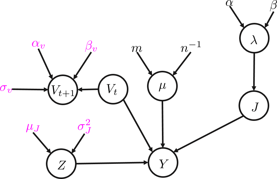
Figure 1: Jusm Stochastic Volatility Model as a Graphical model

We see, that the jump sizes depend on the magnitude of the current volatility $V_{t}$. Thus, the state variables $(J_{t},Z_{t},V_{t})$ are defined by two parameters $\Theta=(\mu,\lambda)$. At the same time the distribution of $\Theta$ is defined by the hyperparameters that have sufficient statistics $s_{t}=(m_{t},n_{t},\alpha_{t},\beta_{t})$, which we denote by $\Theta\sim p(\Theta|s_{t})$. We now construct the conditional posterior distribution of the parameter $\mu$. Under a sufficient statistic structure, we have

$$p(\mu|J_{1:t},Z_{1:t},y_{1:t})\equiv p(\mu|s_{t})\sim\mathcal{N}\left(m_{t},n_{t}\right)\;\;{\rm and}\;\;(\lambda|s_{t})\sim Beta(\alpha_{t},\beta_{t})$$

Thus each particle $i$ is defined by $\left\{J_{t},Z_{t},V_{t},s_{t}\right\}^{(i)}$, for $1\leq i\leq N$. Let $\zeta$ denote joint variable $(J_{t+1},V_{t+1},s_{t})$.

The first step is to find the posterior distributions for $\mu$ and $\lambda$. Given $\lambda\sim Beta(\alpha,\beta)$, the posterior is given by

$$\lambda|J_{t+1},s_{t}\sim Beta(\alpha_{t}+J_{t+1},\beta_{t}+1-J_{t+1})$$

with an update value for hyper parameters

$$\alpha_{t+1}=\alpha_{t}+J_{t+1},\ \beta_{t+1}=\beta_{t}+1-J_{t+1}$$

Now we look at $p(Y_{t}|Z_{t},J_{t},\mu,\lambda)$. Note, that $J_{t}Z_{t}\sim N(J_{t}\mu_{J},J_{t}\sigma_{J})$ and independent of $\epsilon_{t}$. Thus we can easily marginalize $Z_{t}$ using sum of normal variables formula, and obtain

$$y_{t}= \mu+J_{t}\mu_{J}+\sqrt{J_{t}\sigma_{J}^{2}+V_{t}}\epsilon_{t}$$

$$Y_{t}|\Theta,J_{t}\sim N(\mu+J_{t}\mu_{J},\sqrt{J_{t}\sigma_{J}^{2}+V_{t}})$$

We denote the precision parameter by $\gamma_{t}=\dfrac{1}{J_{t}\sigma_{J}^{2}+V_{t}}$ and $Q_{t+1}=y_{t+1}-J_{t+1}\mu_{J}$.

Now, the joint distribution for $\mu$ and $y_{t+1}$ is given by

$$p(y_{t+1},\mu|\zeta_{t})=p(y_{t+1}|\mu,\zeta_{t})p(\mu|s_{t})=p(\mu|y_{t+1},\zeta_{t})p(y_{t+1}|\zeta_{t})$$

$$p(y_{t+1}|\mu,\zeta_{t})=\frac{\sqrt{\gamma_{t+1}}\exp\left(-\frac{1}{2}\gamma_{t+1}\left(\mu-Q_{t+1}\right){}^{2}\right)}{\sqrt{2\pi}}$$

and

$$p(\mu|s_{t})=\frac{\sqrt{n_{t}}\exp\left(-\frac{1}{2}n_{t}\left(\mu-m_{t}\right){}^{2}\right)}{\sqrt{2\pi}}$$

$$p(y_{t+1},\mu|\zeta_{t})\propto\exp\left(-\frac{1}{2}\gamma_{t+1}\left(\mu-Q_{t+1}\right){}^{2}\right)\exp\left(-\frac{1}{2}n_{t}\left(\mu-m_{t}\right){}^{2}\right).$$

On the other hand

$$p(\mu|y_{t+1},\zeta_{t})p(y_{t+1}|\zeta_{t})\propto\exp\left(-\frac{1}{2}n_{t+1}\left(\mu-m_{t+1}\right){}^{2}\right)\exp\left(-\frac{1}{2}\tau_{t+1}\left(\mu-Q_{t+1}\right){}^{2}\right)$$

To calculate mean and standard deviation of the predictive likelihood $p(y_{t+1}|\zeta_{t})$ and posterior for mean $p(\mu|y_{t+1},\zeta_{t})$, we use the identity

$$\frac{\left(x-\mu_{1}\right){}^{2}}{\sigma_{1}}+\frac{\left(x-\mu_{2}\right){}^{2}}{\sigma_{2}}=\frac{\left(\mu_{1}-\mu_{2}\right){}^{2}}{\sigma_{1}+\sigma_{2}}+\frac{\left(x-\mu_{3}\right){}^{2}}{\sigma_{3}}$$

$$\mu_{3}\ =\sigma_{3}\left(\frac{\mu_{1}}{\sigma_{1}}+\frac{\mu_{2}}{\sigma_{2}}\right),~{}\sigma_{3}=\frac{1}{\frac{1}{\sigma_{2}}+\frac{1}{\sigma_{1}}}.$$

We apply this identity with correspondence $\mu_{1}\rightarrow Q_{t+1}=y_{t+1}-J_{t+1}\mu_{J}$, $\mu_{2}\rightarrow m_{t}$, $\mu_{3}\rightarrow m_{t+1}$, $\sigma_{1}\rightarrow\gamma_{t+1}^{-1}$, $\sigma_{2}\rightarrow n_{t}^{-1}$, $\sigma_{3}\rightarrow n_{t+1}^{-1}$, and $\sigma_{1}+\sigma_{2}\rightarrow\tau_{t+1}^{-1}$.

From this we can calculate the updates for the hyper parameters as follows

$$m_{t+1}=\frac{n_{t}}{n_{t}+\gamma_{t+1}}m_{t}+\frac{\gamma_{t+1}}{n_{t}+\gamma_{t+1}}Q_{t+1}=\frac{n_{t}m_{t}+\gamma_{t+1}Q_{t+1}}{n_{t}+\gamma_{t+1}},\ n_{t+1}=n_{t}+\gamma_{t+1},$$

The predictive distribution is given by

$$p(y_{t+1}|\zeta_{t})\propto\exp\left(-\frac{\left(Q_{t+1}-m_{t}\right){}^{2}}{2\left(\frac{1}{n_{t}}+\frac{1}{\gamma_{t+1}}\right)}\right).$$

The likelihood precision is $\tau_{t+1}=\frac{n_{t}\gamma_{t+1}}{n_{t}+\gamma_{t+1}}$, and by normalizing, we obtain

$$p(y_{t+1}|\zeta_{t})=\phi(J_{t+1}\mu_{J}+m_{t},\tau_{t+1}^{-1}).$$

The predictive likelihood $p(y_{t+1}|V_{t+1},s_{t})$ is determined by summing out $J_{t+1}$ as

$$p(y_{t+1}|V_{t+1},s_{t})=\sum_{J_{t+1}\in\{0,1\}}p(y_{t+1}|J_{t+1},V_{t+1},s_{t})p(J_{t+1}|s_{t}),$$ (1)

where

$$p(J_{t+1}=0|s_{t}) =\frac{\alpha_{t}}{\alpha_{t}+\beta_{t}}\mbox{ and }p(J_{t+1}=1|s_{t})=\frac{\beta_{t}}{\alpha_{t}+\beta_{t}}$$

$$p(y_{t+1}|J_{t+1}=0,V_{t+1},s_{t}) =\phi(m_{t},n_{t}^{-1}+V_{t+1})$$

$$p(y_{t+1}|J_{t+1}=1,V_{t+1},s_{t}) =\phi(\mu_{J}+m_{t},n_{t}^{-1}+\sigma_{J}^{2}+V_{t+1}).$$

Finally, we need to find formulas for propagating the state vector $(J_{t},Z_{t},V_{t})$, given the latest observation $y_{t+1}$. Note, that $V_{t+1}$ is conditionally independent of $y_{t+1}$, given $V_{t}$. Thus, we can propagate the volatility variable by draying from the truncated normal $V_{t+1}\sim\mathcal{TN}\left(\alpha_{v}+\beta_{v}V_{t},\sigma_{v}\sqrt{V_{t}}\right)$.

The odds ratio for $J_{t+1}$, is given by

$$\frac{p(J_{t+1}=0|y_{t+1},V_{t+1},s_{t})}{p(J_{t+1}=1|y_{t+1},V_{t+1},s_{t})} =\frac{p(y_{t+1}|J_{t+1}=0,V_{t+1},s_{t})}{p(y_{t+1}|J_{t+1}=1,V_{t+1},s_{t})}\frac{p(J_{t+1}=0|s_{t})}{p(J_{t+1}=1|s_{t})}$$

$$=\frac{\phi(m_{t},n_{t}^{-1}+V_{t+1})}{\phi(\mu_{J}+m_{t},n_{t}^{-1}+\sigma_{J}^{2}+V_{t+1})}\frac{\alpha_{t}}{\beta_{t}}$$

If we sample $J_{t+1}=0$, then size of the jump $Z_{t+1}$ is irrelevant, otherwise we have

$$Z_{t+1}=y_{t+1}-m_{t}+\sqrt{n^{-1}_{t}+\sigma_{J}^{2}+V_{t+1}}\epsilon_{t}$$

Thus, the posteriors is

$$p(Z_{t+1}|y_{t+1},J_{t+1}=1,V_{t+1},s_{t})=\phi(y_{t+1}-m_{t},n^{-1}_{t}+\sigma_{J}^{2}+V_{t+1})$$

This leads to the following algorithm

1. Resample index $k_{t+1}^{(i)}\sim Mult\left\{p\left(y_{t+1}|(V_{t+1},s_{t})^{(i)}\right)\right\}$, so that $(V_{t+1},s_{t})^{k_{t+1}^{(i)}}\sim p(V_{t},s_{t}|y_{1:t+1})$

2. Propagate $Z_{t}^{k_{t+1}^{(i)}}$ and $J_{t}^{k_{t+1}^{(i)}}$, using equations (2.2) and (2.2) correspondingly

3. Update sufficient statistics $s_{t+1}^{i}=S\left(s_{t}^{k_{t+1}^{(i)}}\right)$, using equations (2.2) and 2.2.

4. Propagate volatilities by drawing $V_{t+2}\sim\mathcal{TN}\left((1-\beta_{v})\alpha_{v}+\beta_{v}V_{t+1},\sigma_{v}\sqrt{V_{t+1}}\right)$

3 Application: Google stock returns

We now implement our particle filtering and learning algorithm. Namely, we applied the algorithm to the 1929 Google and S&P500 daily stock returns from January 3 2007 to August 29, 2014. Table 1 provides summary statistics for the returns.

	Mean	Std. Deviation	Skewness	Kurtosis	Min	Max
Google	4.84e-04	0.0193	0.21	8.7	-0.123	0.161
S&P500	1.78e-04	0.0135	-0.383	9.35	-0.0911	0.101

Table 1: Summary statistics for the daily log-returns

As expected, the daily returns exhibit a large amount of kurtosis consistent with time varying second moments, as in stochastic volatility or jumps. Figure 2 below shows the price and return data for the selected period, confirming the time variation in volatility.

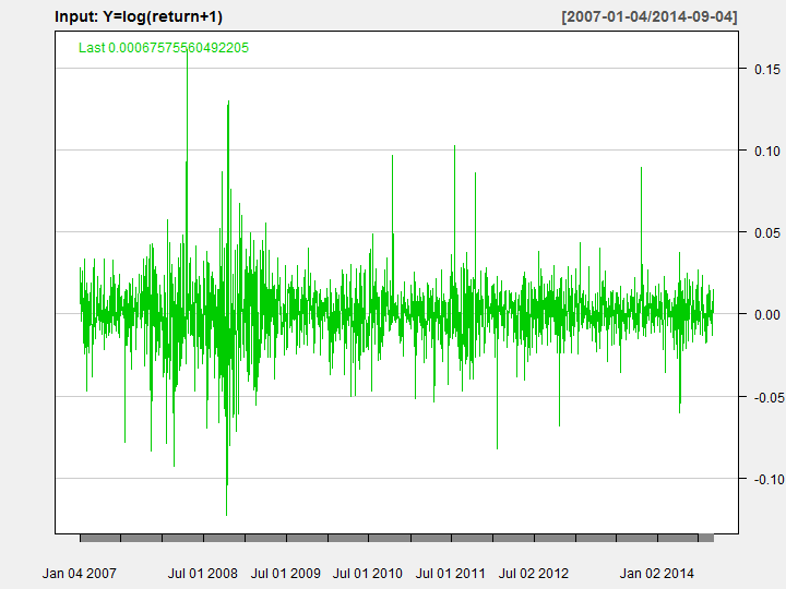
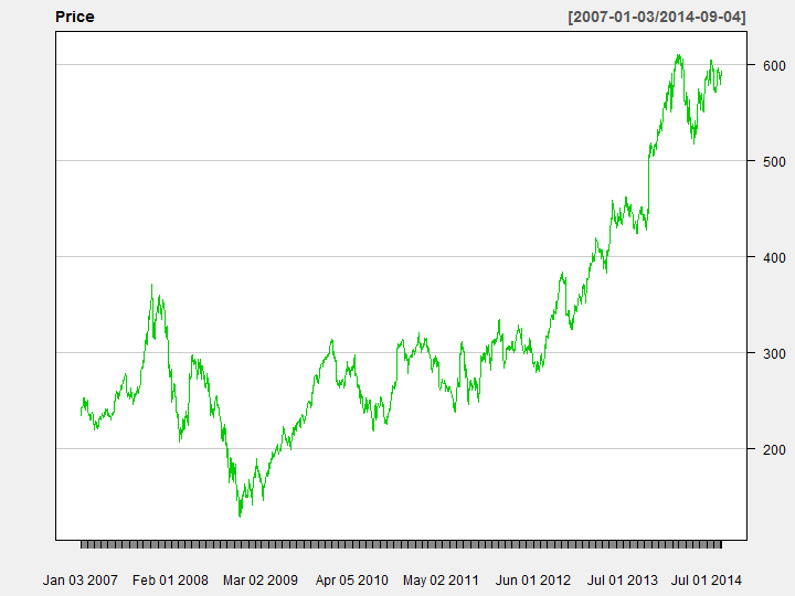
(a) GOOGLE Daily Log-returns	(b) GOOGLE Daily Price
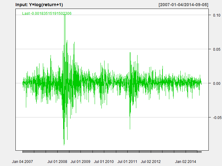
(c) S&P500 Daily Log-returns	(d) S&P500 Daily Price

Figure 2: Price and return data for Google stock

Tables 2 and 3 provides posterior means and standard deviation of the parameters and state variables for the models estimated, as well as prior values. The second and fourth columns provide parameter posterior means, and standard deviations in parentheses, for the Merton and Merton-SV models.

	Prior (Merton)	Posterior (Merton)	Prior (Merton-SV)	Posterior (Merton-SV)
$\mu_{J}$	-0.04		-0.04
$\sigma^{2}_{J}$	1
$\mu$	0.003	3.86e-03 (9.52e-04)	0.003	1.57e-03 (2.96e-03)
$\sigma^{2}$	0.001	1.49e-04 (3.97e-05)	0.01	1.35e-04 (7.94e-04)
$\lambda$	0.09	0.086(0.219)	0.5	7.15e-03 (0.0266)
$Z$		-0.0399 (8.62e-03)		-0.0397 (0.0413)
$\alpha_{v}$			0.0016
$\beta_{v}$			0.99
$V$			0.3	0.237 (0.0336)

Table 2: Parameter Estimates and Priors fro Google

	Prior (Merton)	Posterior (Merton)	Prior (Merton-SV)	Posterior (Merton-SV)
$\mu_{J}$	-0.04		-0.04
$\sigma^{2}_{J}$	1
$\mu$	0.003	2.77e-03(7.8e-04)	0.003	3.62e-04 (1.98e-03)
$\sigma^{2}$	0.001	7.05e-05 (2.62e-05)	0.01	1.3e-04 (7.4e-04)
$\lambda$	0.09	0.0627 (0.213)	0.5	0.011 (0.0542)
$Z$		-0.0398 (1.93e-03)		-0.0417 (0.0395)
$\alpha_{v}$			0.0016
$\beta_{v}$			0.99
$V$			0.3	0.216 (0.0374)

Table 3: Parameter Estimates and Priors fro S&P 500

Consider the pure Merton model without stochastic volatility. Figure 3 shows the filtered state parameters $Z$ ans $J$ estimated using the Merton jump model. We can see that the cluster of jumps in July 2008. Such a clustering indicates that the model may be misspecified. One reason for that is that the volatility is fixed in the model and thus, all of the large moves on returns are attributed to jumps. However, the clustering of jumps is extremely unlikely in reality due to the i.i.d assumption on the jump time and size specification and infrequent nature of jumps.

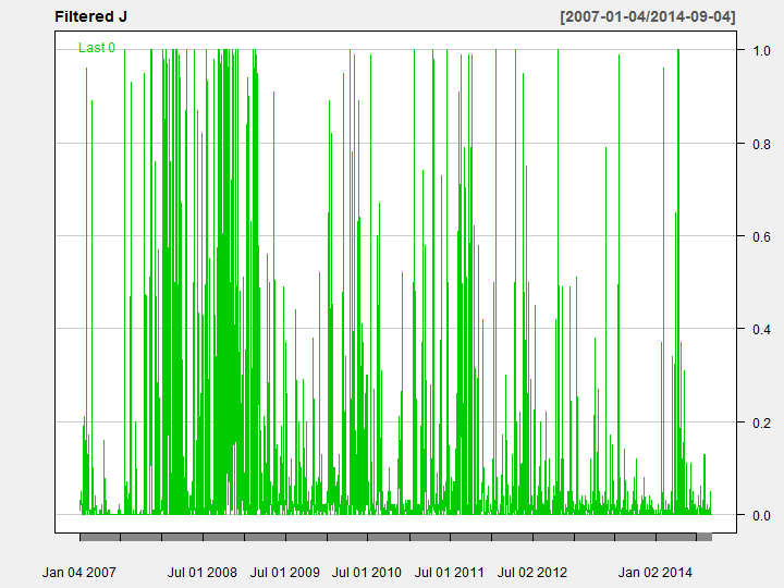
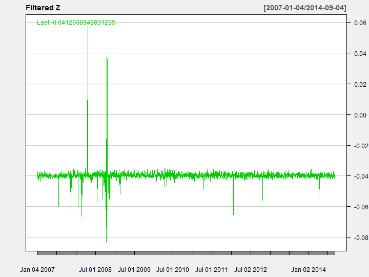
(a) Filtered J for GOOGLE	(b) Filtered Z for GOOGLE
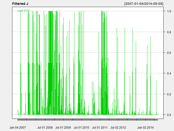
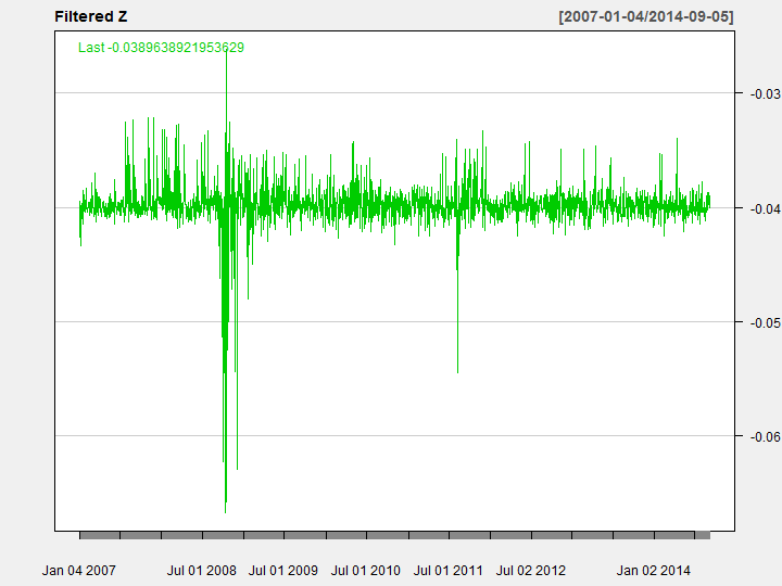
(a) Filtered J for S&P500	(b) Filtered Z for S&P500

Figure 3: Value of the filtered state variables for Merton model

These clustered jumps of 2008 in fact reflect higher volatility of returns.

The fourth column of Tables 2 and 3 provides the parameters estimates for the Merton-SV model. Adding stochastic volatility to the jump model has the expected effect of reducing the amount of jumps in the returns. Virtually, all of the changes on returns are explained by the stochastic volatility

4 Discussion

Particle filtering methods are flexible and fast to compute. They provide a simple solution to the sequential inference problem where Markov Chain Monte Carlo (MCMC) are computationally expensive as they have to be re-run every time a new data point arrives. We develop and implement a particle filtering and learning algorithm that provides full inference for Merton’s jump stochastic volatility model. To perform sequential parameter learning we exploit a conditional sufficient statistic state variable that we filter with particle methods and then we draw parameters in an off line fashion. This provides an efficient approach to parameter inference.

There are a number of possible extensions of our work. On the finance side, there are many models with a similar nature to Merton’s original specification such as the Leland and Toft (1996) model of corporate credit. These models are state space-models and are amenable to particle filtering methods. On the econometrics side, extensions to continuous-time jump diffusions (Johannes et al. (2009) with infinite activity jumps (Li et al. (2008)) or to self-exciting jump processes (Fulop et al. (2012); Aït-Sahalia and Jacod (2009, 2012)) is an avenue for future study. Incorporating a leverage effect (or correlated errors) together with multivariate models is another area of interest (Jacquier et al. (1995, 2004)). We leave these as avenues for future study.

We intent to extend our analysis to currencies (FX) and security portfolios (e.g. market indexes). Furthermore, we will demonstrate both computational accuracy of estimation differences between particle filters and MCMC based methods.

Appendix A: Particle Filtering Methods

State space models (Carlin et al. (1992); Duffie (1996); Johannes and Polson (2010)) are central to inference in financial econometrics. Particle filtering methods are designed to provide state inference (Gordon et al. (1993); Carpenter et al. (1999); Pitt and Shephard (1999); Storvik (2002); Carvalho et al. (2010)).

Let $y_{t}$ denote the data, and $\theta_{t}$ the state variable. For example, in Merton’s jump stochastic volatility model, the state variable is $(J_{t},Z_{t},V_{t})$, corresponding to the jump times and sizes and stochastic volatility. Let $\phi$ denote the unknown parameters relating to the dynamics of the underlying jump and stochastic volatility distributions. For the moment, we suppress the conditioning on the parameters $\phi$. We now show how a PF algorithm updates state variables.

We can factorize the joint posterior distribution of the data and state variables both ways as

$$p(y_{t+1},\theta_{t+1}|\theta_{t}) =p(y_{t+1}|\theta_{t+1})p(\theta_{t+1}|\theta_{t})$$

$$=p(y_{t+1}|\theta_{t})\,p(\theta_{t+1}|\theta_{t},y_{t+1})$$

The goal is to obtain the new filtering distribution $p(\theta_{t+1}|y^{t+1})$ from the current $p(\theta_{t}|y^{t})$. A particle representation of the previous filtering distribution is a random histogram of draws. We denote this by

$$p^{N}(\theta_{t}|y^{t})=\frac{1}{\,N\,}\sum_{i=1}^{N}\delta_{\theta_{t}^{(i)}}.$$

where $\delta$ is a Dirac measure. As the number of particles increases $N\rightarrow\infty$ the law of large numbers guarantees that this distribution converges to the true filtered distribution $p(\theta_{t}|y^{t})$.

In order to provide random draws of the next distribution, we first resample $\theta_{t}$’s using the smoothing distribution obtained by Bayes rule.

$$p(\theta_{t}|y^{t+1})\propto p(y_{t+1}|\theta_{t})p(\theta_{t}|y^{t})$$

Thus, we draw $\theta^{k(i)}_{t}$ via an index $k(i)$ from a multinomial with weights

$$w^{(i)}_{t}=\frac{p(y_{t+1}|\theta_{t}^{(i)})}{\sum_{j=1}^{N}p(y_{t+1}|\theta_{t}^{(j)})}.$$

We set $\theta^{(i)}_{t}=\theta^{k(i)}_{t}$ and “propagate” to the next time $t+1$ using

$$p(\theta_{t+1}|y_{1:t+1})=\int p(\theta_{t+1}|\theta_{t},y_{t+1})p(\theta_{t}|y_{1:t+1})d\theta_{t}.$$

Given a particle approximation $\{\theta^{(i)}:1\leq i\leq N\}$ to $p^{N}\left(\theta_{t}|y^{t}\right)$, we can use Bayes rule to write

$$p^{N}\left(\theta_{t+1}|y^{t+1}\right) \propto\sum_{i=1}^{N}p\left(y_{t+1}|\theta_{t}^{\left(i\right)}\right)p\left(\theta_{t+1}|\theta_{t}^{\left(i\right)},y_{t+1}\right)$$

$$=\sum_{i=1}^{N}w_{t}^{\left(i\right)}p\left(\theta_{t+1}|\theta_{t}^{\left(i\right)},y_{t+1}\right)\text{,}$$

where the particle weights are given by

$$w_{t}^{\left(i\right)}=\frac{p\left(y_{t+1}|\theta_{t}^{\left(i\right)}\right)}{\sum_{i=1}^{N}p\left(y_{t+1}|\theta_{t}^{\left(i\right)}\right)}\text{.}$$

This mixture distribution representation leads to a simple simulation approach for propagating particles to the next filtering distribution.

The algorithm consists of two steps:

$$\text{Step 1. (Resample) Draw }\theta_{t}^{\left(i\right)}\sim Mult_{N}\left(w_{t}^{\left(1\right)},...,w_{t}^{\left(N\right)}\right)\text{ for }i=1,...,N$$

$$\text{Step 2. (Propagate) Draw }\theta_{t+1}^{\left(i\right)}\sim p\left(\theta_{t+1}|\theta_{t}^{\left(i\right)},y_{t+1}\right)\text{ for }i=1,...,N.$$

To implement this algorithm, we need the predictive likelihood for the next observation, $y_{t+1}$, given the current state variable $\theta_{t}$. It is defined by

$$p\left(y_{t+1}|\theta_{t}\right)=\int p\left(y_{t+1}|\theta_{t+1}\right)p\left(\theta_{t+1}|\theta_{t}\right)d\theta_{t+1}.$$

We also need the conditional posterior for the next states $\theta_{t+1}$ given $(\theta_{t},y_{t+1})$, given by

$$p\left(\theta_{t+1}|\theta_{t},y_{t+1}\right)\propto p\left(y_{t+1}|\theta_{t+1}\right)p\left(\theta_{t+1}|\theta_{t}\right)\;.$$

Our algorithm has several practical advantages. First, it does not suffer from the problem of particle degeneracy which plagues the standard sample-importance resample filtering algorithms. This effect is heightened when $y_{t+1}$ is an outlier. Second, it can easily be extended to incorporate sequential parameter learning. It is common to also require learning about other unknown static parameters, denoted by $\phi$. To do this, we assume that there exists a conditional sufficient statistic $s_{t}$ for $\phi$ at time$\,t$, namely

$$p(\phi|\theta_{1:t},y_{1:t})=p(\phi|s_{t})$$

where $s_{t}=s(\theta_{1:t},y_{1:t})$. Moreover, we can propagate these sufficient statistics by the deterministic recursion $s_{t+1}=S(s_{t},\theta_{t+1},y_{t+1})$ In the next section we develop the sufficient statistics and appropriate recursions for Merton’s jump stochastic volatility model. This will lead to efficient inference for all model parameters.

Given particles $(\theta_{t},\phi,s_{t})^{(i)},$ $i=1,\ldots,N$. First, we resample $(\theta_{t},\phi,s_{t})^{k(i)}$ with weights proportional to $p(y_{t+1}|(\theta_{t},\phi)^{k(i)})$. Then we propagate to the next filtering distribution $p(\theta_{t+1}|y_{1:t+1})$ by drawing $\theta^{(i)}_{t+1}\,$from $p(\theta_{t+1}|\theta^{k(i)}_{t},\phi^{k(i)},y_{t+1}),\,i=1,\ldots,N$. We next update the sufficient statistic for $i=1,\ldots,N$,

$$s_{t+1}=S(s_{t}^{k(i)},\theta^{(i)}_{t+1},y_{t+1}),$$

This represents a deterministic propagation. Parameter learning is completed by drawing $\phi^{(i)}$ using $p(\phi|s^{(i)}_{t+1})$ for $i=1,\ldots,N$. We now gives specifics of the algorithm for two models, the Merton model with constant and stochastic volatility. We now track the state, $\theta_{t}$, and conditional sufficient statistics, $s_{t}$, which will be used to perform off-line learning for $\phi$.

The algorithm now consists of four steps:

$$\text{Step 1. (Resample) Draw Index }k_{t}(i)\sim Mult_{N}\left(w_{t}^{\left(1\right)},...,w_{t}^{\left(N\right)}\right)\text{ for }i=1,...,N$$

$$\text{The weights are proportional to }p(y_{t+1}|(\theta_{t},s_{t})^{(i)})$$

$$\text{Step 2. (Propagate) Draw }\theta_{t+1}^{\left(i\right)}\sim p\left(\theta_{t+1}|(\theta_{t},s_{t})^{k\left(i\right)},y_{t+1}\right)\text{ for }i=1,...,N.$$

$$\text{Step 3. (Update) Deterministic }s_{t+1}^{\left(i\right)}=S\left(s_{t}^{k(i)},\theta_{t+1}^{(i)},y_{t+1}\right)\text{ for }i=1,...,N.$$

$$\text{Step 4. (Learning) Offline }\phi^{\left(i\right)}\sim p\left(\phi|s_{t+1}^{(i)}\right)\text{ for }i=1,...,N.$$

References

Aït-Sahalia and
Jacod (2009)
Aït-Sahalia, Y. and J. Jacod
2009.
Estimating the degree of activity of jumps in high frequency data.
The Annals of Statistics, Pp. 2202–2244.
Aït-Sahalia and
Jacod (2012)
Aït-Sahalia, Y. and J. Jacod
2012.
Analyzing the spectrum of asset returns: Jump and volatility
components in high frequency data.
Journal of Economic Literature, 50(4):1007–1050.
Carlin et al. (1992)
Carlin, B. P., N. G. Polson, and D. S. Stoffer
1992.
A Monte Carlo approach to nonnormal and nonlinear state-space
modeling.
Journal of the American Statistical Association,
87(418):493–500.
Carpenter et al. (1999)
Carpenter, J., P. Clifford, and P. Fearnhead
1999.
Improved particle filter for nonlinear problems.
IEE Proceedings-Radar, Sonar and Navigation, 146(1):2–7.
Carvalho et al. (2010)
Carvalho, C., M. S. Johannes, H. F. Lopes, and
N. Polson
2010.
Particle learning and smoothing.
Statistical Science, 25(1):88–106.
Dubinsky and Johannes (2005)
Dubinsky, A. and M. Johannes
2005.
Earnings announcements and equity options.
Working Paper.
Duffie (1996)
Duffie, D.
1996.
State-space models of the term structure of interest rates.
In Stochastic Analysis and Related Topics V, Pp.
41–67.
Springer.
Duffie et al. (2000)
Duffie, D., J. Pan, and K. Singleton
2000.
Transform analysis and asset pricing for affine jump-diffusions.
Econometrica, 68(6):1343–1376.
Eraker et al. (2003)
Eraker, B., M. Johannes, and N. Polson
2003.
The impact of jumps in volatility and returns.
The Journal of Finance, 58(3):1269–1300.
Fulop et al. (2012)
Fulop, A., J. Li, and J. Yu
2012.
Bayesian learning of impacts of self-exciting jumps in returns and
volatility.
Working Paper.
Gordon et al. (1993)
Gordon, N. J., D. J. Salmond, and A. F. Smith
1993.
Novel approach to nonlinear/non-Gaussian Bayesian state
estimation.
In IEE Proceedings F-Radar and Signal Processing,
volume 140, Pp. 107–113. IET.
Jacquier et al. (2004)
Jacquier, E., N. Polson, and P. Rossi
2004.
Bayesian Inference for SV models with Correlated Errors.
Journal of Econometrics.
Jacquier et al. (1995)
Jacquier, E., N. G. Polson, and P. E. Rossi
1995.
Models and priors for multivariate stochastic volatility.
Working paper, University of Chicago.
Johannes and Polson (2009)
Johannes, M. and N. Polson
2009.