Gluing Affine Vortices

Abstract.

We construct a gluing map for stable affine vortices over the upper half plane with the Lagrangian boundary condition at a rigid, regular, codimension one configuration. This construction plays an important role in establishing the relation between the gauged linear sigma model and the nonlinear sigma model in the presence of Lagrangian branes.

2010 Mathematics Subject Classification: 53D40

Keywords: vortex equation, gluing, adiabatic limits, holomorphic disks, gauged linear sigma model (GLSM)

1. Introduction

The vortex equation is a first-order elliptic equation whose solutions, called vortices, appear in many different areas of mathematics and physics. In physics, vortices first showed up in the Ginzburg–Landau theory in superconductivity (see [8] [15] [9]), and reappeared in many other more abstract physical theories such as the gauged linear sigma model (GLSM) [29]. In mathematics, especially in symplectic geometry, vortices play the role as equivariant generalizations of pseudoholomorphic curves. Enumerations of vortices lead to the definition of the gauged Gromov–Witten invariants (see [12, 3, 13, 2]) and Floer-type theories (see [5] [33]). The generalization of the vortex equation, called the gauged Witten equation, plays a fundamental role in the author’s project with Tian on a mathematical theory of the GLSM (see [19, 17, 21, 18, 20]).

An important argument in the vortex theory is the adiabatic limit. In the adiabatic limit, vortices converge to pseudoholomorphic curves. This phenomenon leads several important results and conjectures. Using the adiabatic limit, Gaio–Salamon [7] relates certain gauged Gromov–Witten invariants and the usual Gromov–Witten invariants. Moreover, they conjecture that a more general relation between these two types of invariants should lead to a quantization of the Kirwan map in a similar way as the Gromov–Witten invariants quantize the multiplicative structure of the cohomology ring. In gauge theory the adiabatic limit argument for the instanton equation leads to Dostoglou–Salamon’s proof of the $SO(3)$ Atiayh–Floer conjecture for mapping cylinders [4].

In the adiabatic limit the convergence of vortices towards holomorphic curves generally should be “corrected” by taking into account the contribution of certain bubbles. These bubbles are called affine vortices or pointlike instantons. Their contributions, often nontrivial, have already been pointed out by Witten [29] in the context of the GLSM. Similar to counting pseudoholomorphic curves, to define the contributions of affine vortices, one needs to compactify their moduli spaces and construct manifold-like structures (such as Kuranishi structures) over the moduli space. The compactness results for affine vortices (see [35, 37] and [25]) and the stratification of the domain moduli (see [10]) indicate that the involved gluing construction should differ from the gluing of holomorphic curves.

In this paper we construct the gluing map for affine vortices over the upper half plane satisfying a Lagrangian boundary condition. Instead of working in the most general situation, we restrict to the case when the singular configuration lies in a codimension one stratum of the compactified moduli space and when the singular configuration is rigid. A practical reason for having this restriction is that this is what one needs in the related work [31] where the authors construct an open version of the quantum Kirwan map. The construction in more general situations will be considered elsewhere. For example, in the forthcoming work [16] a general gluing construction will be provided for pointlike instantons (with nontrivial superpotentials but without a boundary condition) over the complex plane, giving local Kuranishi model on the relevant moduli space.

Our main theorem is the following, whose precise version is restated as Theorem 3.3.

Theorem 1.1.

Let $(V,\omega,\mu)$ be a Hamiltonian $K$-manifold. Assume that the symplectic quotient $X:=\mu^{-1}(0)/K$ is a free quotient. Let $L_{V}\subset V$ be a $K$-invariant embedded Lagrangian submanifold which is contained in $\mu^{-1}(0)$.

Given nonnegative integers $l,l^{+}$ with $l+l^{+}\geq 1$, let $\overline{\mathcal{M}}_{l,l^{+}}(V,L_{V})$ be the moduli space of gauge equivalence classes of stable affine vortices over ${\mathbb{H}}$ with $l$ boundary marked points and $l^{+}$ interior marked points (with respect to a given family of domain-dependent almost complex structure), equipped with a natural topology. Let $\Gamma$ be a simple combinatorial type (see Definition 2.18) which labels a codimension one stratum ${\mathcal{M}}_{\Gamma}(V,L_{V})\subset\overline{\mathcal{M}}_{l,l^{+}}(V,L_{V})$.

Given a regular and rigid point ${\bm{p}}\in{\mathcal{M}}_{\Gamma}(V,L_{V})$ (see Definition 3.2), there exists an open neighborhood of ${\bm{p}}$ in $\overline{\mathcal{M}}_{l,l^{+}}(V,L_{V})$ which is homeomorphic to the interval $[0,\epsilon)$.

Our proof is conceptually straightforward and follows a standard protocol used in gauge theory and symplectic geometry. However the complicated behavior of vortices and some subtle features make the argument rather involved. On the technical level, one can view our construction as a nontrivial generalization of the case of Gaio–Salamon [7] in two different ways. First, the singular configuration we would like to glue consists of two types of components, affine vortices or holomorphic curves, while in the case of [7] they only need to treat limiting configurations which are smooth holomorphic curves. Second, while Gaio–Salamon only treated the vortex equation over compact domains, the noncompact domain of the vortex equation considered here requires particular choices of weighted Sobolev norms and a slightly atypical local model theory (see [23]). With these two types of complications combined, to ensure the gluing protocol can be operated, we need to make extra effort to arrange various ingredients more carefully.

1.1. Extensions and applications

As we have explained, the immediate motivation for studying the gluing of affine vortices is from the project of the author with Woodward [31], aiming at defining an “open quantum Kirwan map.” The open quantum Kirwan map is a morphism of $A_{\infty}$ algebras from the quasimap Fukaya $A_{\infty}$ algebra of $L_{V}$ to a bulk-deformed Fukaya $A_{\infty}$ algebra of the Lagrangian in the quotient $X$.

Moreover, using the technique and the analytical setting of this paper, one can construct the gluing map for affine vortices over ${\mathbb{C}}$, and the gluing map with respect to the adiabatic limit. This would be an important step towards the resolution of Salamon’s quantum Kirwan map conjecture in the symplectic setting, initiated in [35] [37] (proved by Woodward [30] in the algebraic case). If one allows a nontrivial superpotential in the general setting of the GLSM, where affine vortices are often referred to as pointlike instantons, then the corresponding gluing construction is necessary to establish a relation between the GLSM correlation functions and Gromov–Witten invariants. This is part of the on-going project of the author with G. Tian [16].

One specific feature of the affine vortex equation is that the equation has only translation invariance but not conformal invariance. In symplectic geometry and gauge theory there are other types of objects which have the same symmetry types. The figure-eight bubble, appeared in the strip shrinking limits of pseudoholomorphic quilts (see [27] [28] [1]), is such an example. There are also examples in gauge theory, such as the anti-self-dual equation or the monopole equation over ${\mathbb{C}}\times\Sigma$ (see [26] and [24]) and over the product of the real line with a noncompact three-manifold with cylindrical ends (see [34]). We hope that the technique of this paper can be used in the gluing construction for other translation invariant equations.

1.2. Acknowledgments

I would like to thank Chris Woodward for many stimulating discussions and his generosity in sharing ideas. I would also like to thank Gang Tian and Kenji Fukaya for their support and encouragements, and thank Sushmita Venugopalan for helpful discussions.

2. Affine Vortices and Their Moduli

In this section we review the basic facts about affine vortices and their moduli spaces. We also set up notations for trees, domain-dependent almost complex structures, and local models of the domain moduli.

2.1. Preliminaries on affine vortices

We first recall basic knowledge of affine vortices and fix some notations. Let $K$ be a compact Lie group with its Lie algebra ${\mathfrak{k}}$ and its complexification $G$. Let $(V,\omega_{V})$ be a symplectic manifold with a smooth $K$-action. For each $\eta\in{\mathfrak{k}}$, let ${\mathcal{X}}_{\eta}\in{\mathit{\Gamma}}(TV)$ be the infinitesimal action. Our convention is that the map $\eta\mapsto{\mathcal{X}}_{\eta}$ is an anti-homomorphism of Lie algebras from ${\mathfrak{k}}$ to ${\mathit{\Gamma}}(TV)$. Assume that the $K$-action is Hamiltonian and has a moment map

$$\mu:V\to{\mathfrak{k}}^{*}.$$

This means that $\mu$ is $K$-equivariant and satisfies

$$\langle d\mu(Z),\eta\rangle=\omega_{V}({\mathcal{X}}_{\eta},Z),\ \forall\eta\in{\mathfrak{k}},\ Z\in TV.$$

We make the following basic assumption.

Hypothesis 2.1.

$0\in{\mathfrak{k}}$ is a regular value of $\mu$ and the symplectic quotient $X:=\mu^{-1}(0)/K$ is a free quotient.

Now we recall the notion of gauged maps and vortices. Let $\Sigma$ be a Riemann surface with possibly nonempty boundary. A gauged map from $\Sigma$ to $V$ is a triple ${\bm{v}}=(P,A,u)$ where $P\to\Sigma$ is a smooth $K$-bundle, $A\in{\mathcal{A}}(P)$ is a connection, and $u\in{\mathit{\Gamma}}(P(V))$ is a smooth section. Here $P(V)=(P\times V)/K$ is the associated fibre bundle. To a gauged map ${\bm{v}}=(P,A,u)$ one has the following associated objects:

• the curvature $F_{A}\in\Omega^{2}(\Sigma,{\rm ad}P)$,

• the moment potential $\mu(u)\in\Omega^{0}(\Sigma,({\rm ad}P)^{*})$, and

• the covariant derivative $d_{A}u\in\Omega^{1}(\Sigma,u^{*}P(TV))$.

Suppose $\Sigma$ is equipped with an area form $\nu_{\Sigma}$, which, together with the complex structure on $\Sigma$, determines a metric on $\Sigma$. Suppose $V$ is equipped with a $K$-invariant Riemannian metric and the Lie algebra ${\mathfrak{k}}$ is equipped with an invariant inner product. We define the energy of the gauged map ${\bm{v}}=(P,A,u)$ to be

$$E({\bm{v}})=E(P,A,u):=\frac{1}{2}\left(\|d_{A}u\|_{L^{2}(\Sigma)}^{2}+\|F_{A}\|_{L^{2}(\Sigma)}^{2}+\|\mu(u)\|_{L^{2}(\Sigma)}^{2}\right).$$

The vortex equation is the equation of energy minimizers. Suppose the Riemannian metric on $V$ used to define the energy is determined by $\omega_{V}$ and a $K$-invariant $\omega_{V}$-tamed almost complex structure $J$. Then gauged maps minimizing the energy (locally) solve the symplectic vortex equation

$$\ \overline{\partial}_{A}u=0,\ \ *F_{A}+\mu(u)=0.$$ (2.1)

Here $\overline{\partial}_{A}u:=(d_{A}u)^{0,1}$ is the $(0,1)$-part of the covariant derivative with respect to the domain complex structure on $\Sigma$ and the target almost complex structure $J$ on $V$; $*$ is the Hodge star operator on $\Sigma$ determined by the metric on $\Sigma$. The second equation also uses the metric on the Lie algebra to identify ${\rm ad}P\cong({\rm ad}P)^{*}$. We call a solution to (2.1) a symplectic vortex (or simply a vortex) on $\Sigma$.

We will impose a Lagrangian boundary condition for the vortex equation. Let

$$L\subset X$$

be a Lagrangian submanifold, meaning that $\omega_{X}|_{L}\equiv 0$, where $\omega_{X}$ is the symplectic form of the symplectic reduction $X$ induced from $\omega_{V}$. Then the preimage

$$L_{V}\subset\mu^{-1}(0)$$

under the map $\mu^{-1}(0)\to\mu^{-1}(0)/K\subset V$ is a $K$-invariant Lagrangian submanifold of $V$. When $\partial\Sigma\neq\emptyset$, we always impose the following condition for the vortex equation (2.1)

$$u(\partial\Sigma)\subset P(L_{V})\subset P(V).$$ (2.2)

The vortex equation and the boundary condition are invariant under gauge transformations. A gauge transformation on a $K$-bundle $P\to\Sigma$ is a section $g\in{\mathit{\Gamma}}(P(K))$ where $P(K)\to\Sigma$ is the bundle associated to the adjoint action of $K$ on itself. Viewing them as automorphisms of principal bundles, gauge transformations can pull-back connections $A\in{\mathcal{A}}(P)$ and sections $u\in{\mathit{\Gamma}}(P(V))$. We use the notation such that the action by gauge transformations is a left action: for a gauged map ${\bm{v}}=(P,A,u)$, denote

$$g\cdot{\bm{v}}=(P,A\circ g^{-1},\ u\circ g^{-1}).$$

In this paper we only consider gauged maps defined over rather simple domains. These domains are the complex plane ${\mathbb{C}}$, the upper half plane ${\mathbb{H}}$, or their open subsets. Over such a domain there is a standard flat metric and standard complex coordinate $s+{\bm{i}}t$. Let ${\mathbb{A}}$ denote either ${\mathbb{C}}$ or ${\mathbb{H}}$. Then a $K$-bundle $P\to{\mathbb{A}}$ is always trivial; with respect to a trivialization, a gauged map from ${\mathbb{A}}$ to $V$ can be identified with a triple

$${\bm{v}}=(u,\phi,\psi):{\mathbb{A}}\to V\times{\mathfrak{k}}\times{\mathfrak{k}}.$$

Here we identify the connection $A$ with $d+\phi ds+\psi dt$ with respect to the trivialization. In such a gauge, the vortex equation (2.1) is equivalent to

$$\ \partial_{s}u+{\mathcal{X}}_{\phi}(u)+J(\partial_{t}u+{\mathcal{X}}_{\psi}(u))=0,\ \ \partial_{s}\psi-\partial_{t}\phi+[\phi,\psi]+\mu(u)=0$$ (2.3)

and the boundary condition (2.2) is equivalent to

$$u(\partial{\mathbb{A}})\subset L_{V}.$$ (2.4)

Definition 2.2.

An affine vortex over ${\mathbb{C}}$ (resp. ${\mathbb{H}}$) is a finite energy solution ${\bm{v}}=(u,\phi,\psi)$ to (2.3) subject to the boundary condition (2.4). Two affine vortices over ${\mathbb{C}}$ resp. ${\mathbb{H}}$ are isomorphic if after a complex resp. real translation they are gauge equivalent.

One can define a natural topology on the set of isomorphism classes of affine vortices. One can see from the two examples below that this topology cannot be compact.

Example 2.3.

Taubes [14] classifies affine vortices for the simplest target space. Given a complex polynomial $f(z)$, Taubes shows that there exists a unique solution $h:{\mathbb{C}}\to{\mathbb{R}}$ to the Kazdan–Warner equation

$$-\frac{\Delta h}{2\pi}+\frac{1}{2}\left(e^{2h}|f(z)|^{2}-1\right)=0$$

with an appropriate asymptotic condition on $h$. It follows that ${\bm{v}}_{f}:=(e^{h}f,-\partial_{t}h,\partial_{s}h)$ is an affine vortex with target $V={\mathbb{C}}$ acted by $K=U(1)$ with moment map

$$\mu(z)=-\frac{{\bm{i}}}{2}(|z|^{2}-1).$$

One can see how these affine vortices degenerate by looking at the zeroes of the polynomials. Consider a sequence of monic polynomials of degree $d=2$

$$f_{k}(z)=(z-z_{k})(z-z_{k}^{\prime}).$$

Suppose as $k\to\infty$, $|z_{k}-z_{k}^{\prime}|\to\infty$. Then as $k\to\infty$, one can see that the sequence of affine vortices ${\bm{v}}_{f_{k}}$ split into two components. One can viewed such a degeneration as a complex analogue of breaking trajectories in Morse theory.

Example 2.4.

In general, besides splitting into several components, affine vortices can also converge to nontrivial holomorphic maps into the symplectic quotient. One can see this type of limiting behavior in the higher-rank generalization of abelian vortices. For an $N$-tuple of polynomials

$$\vec{f}=(f^{1},\ldots,f^{N}),\ \max_{\alpha}\{{\rm deg}f^{\alpha}\}=d\geq 1,$$

by the main theorem of [32] (see also [22]), there exists a unique solution $h:{\mathbb{C}}\to{\mathbb{R}}$ to the Kazdan–Warner equation

$$-\frac{\Delta h}{2\pi}+\frac{1}{2}\left(e^{2h}\sum_{\alpha=1}^{N}|f^{\alpha}(z)|^{2}-1\right)=0.$$

So such an $N$-tuple of polynomials corresponds to an affine vortex with target $V={\mathbb{C}}^{N}$ acted by the gauge group $K=U(1)$.

A sequence of affine vortices could converge to a holomorphic sphere in the quotient $X=\mathbb{CP}^{N-1}$. Consider the simplest case when $N=2$, $d=1$. Consider a sequence of pairs of polynomials

$$\ f_{k}^{1}(z)=z-k,\ \ f_{k}^{2}(z)=z,\ \ \ k=1,2,\cdots.$$

For the corresponding sequence of affine vortices ${\bm{v}}_{k}=(u_{k},\phi_{k},\psi_{k})$, one can argue that in the $k\to\infty$ limit, if one reparametrize the domain using factor $k$, then $\mu(u_{k})$ converges to zero uniformly and the induced sequence of maps $\bar{u}_{k}:{\mathbb{C}}\to\mathbb{CP}^{1}$ converges to the holomorphic map $z\mapsto[z-1,z]$ into $\mathbb{CP}^{1}$.

We will describe compactifications of moduli spaces of affine vortices in the next subsection. A description relies on the following property of affine vortices.

Proposition 2.5.

[7][36][25] Given an affine vortex ${\bm{v}}=(u,\phi,\psi)$ over ${\mathbb{C}}$ resp. ${\mathbb{H}}$, there is a $K$-orbit $Kx$ in $\mu^{-1}(0)$ resp. in $L_{V}$ such that

$$\lim_{z\to\infty}Ku(z)=Kx\in V/K.$$

The above proposition allows on to define the evaluation at infinity of affine vortices. Given an affine vortex ${\bm{v}}=(u,\phi,\psi)$ over ${\mathbb{C}}$ resp. ${\mathbb{H}}$, its limit at the infinity is denoted by

$${\rm ev}_{\infty}({\bm{v}})\in X\ \ {\rm resp.}\ \ {\rm ev}_{\infty}({\bm{v}})\in L.$$ (2.5)

2.2. Scaled trees and domain moduli

In this section we provide the detailed combinatorial ingredients needed to compactify the moduli space of affine vortices. We first fix the notations about trees. A tree $\Gamma$ has a set of vertices $V_{\Gamma}$ and a set of edges $E_{\Gamma}$. We allow both finite edges, which connect two vertices, and semi-infinite edges, which are only attached to one vertex. Let

$$E_{\Gamma}=E_{\Gamma}^{-}\cup E_{\Gamma}^{\infty}$$

be the decomposition into finite and semi-infinite edges. We always assume that the tree has a distinguished vertex $v_{0}\in V_{\Gamma}$ called the root. The root induces a partial order among vertices: we write $v_{\alpha}\leq v_{\beta}$ if $v_{\alpha}$ is closer to the root. We denote $v_{\beta}\succ v_{\alpha}$ if $v_{\alpha}\leq v_{\beta}$ and these two vertices are adjacent. One can view a tree as a 1-complex in which the semi-infinite edges are open cells. A ribbon tree is a tree $\Gamma$ together with an isotopy class of embeddings $\Gamma\hookrightarrow{\mathbb{R}}^{2}$.

Definition 2.6 (Based tree).

A based tree is a rooted tree $\Gamma$ together with a subtree $\underline{\smash{\Gamma}}{}$ containing the root, a ribbon tree structure on the base, and a bijective labeling

$$\{1,\ldots,l^{+}\}\cong E_{\Gamma}^{\infty}\smallsetminus E_{\underline{\smash{\Gamma}}{}}^{\infty}$$

of semi-infinite edges not in the base.

Notice that semi-infinite edges in the base (representing boundary marked points) are canonically ordered (counterclockwise) and labelled by integers $1,\ldots,l$ via the ribbon tree structure of the base. A based tree can be used to model the combinatorial type of a stable holomorphic disk such that vertices in the base represent disk components and vertices not in the base represent sphere components.

Notation 2.7.

Let $\Gamma$ be a rooted tree.

1. For any edge $e\in E_{\Gamma}$, if $e$ is a finite edge, then let $v_{\alpha(e)}\in V_{\Gamma}$ denote the vertex on one the side of $e$ which is closer to the root; if $e$ is a semi-infinite edge, then let $v_{\alpha(e)}\in V_{\Gamma}$ denote the vertex to which $e$ is attached.

2. Let $V_{\Gamma^{\rm sup}}\subset V_{\Gamma}$ denote the set of vertices not in the base.

To model the combinatorial types of stable affine vortices one needs an extra structure on the tree. A scaling on a rooted tree $\Gamma$ is a map

$${\mathfrak{s}}:V_{\Gamma}\to\{0,1,\infty\}$$

satisfying the following conditions.

1. ${\mathfrak{s}}$ is order-reversing.

2. For any path $v_{1}\succ\cdots\succ v_{k}$ in $\Gamma$, if ${\mathfrak{s}}(v_{1})\leq 1$, ${\mathfrak{s}}(v_{k})\geq 1$, then there is exactly one vertex $v_{l}$ in this path with ${\mathfrak{s}}(v_{l})=1$.

A tree with a scaling is called a scaled tree. We often abbreviate $(\Gamma,{\mathfrak{s}})$ by $\Gamma$. Denote

$$V_{\Gamma}^{0}={\mathfrak{s}}^{-1}(0),\ \hskip 5.69046pt\ V_{\Gamma}^{1}={\mathfrak{s}}^{-1}(1),\ \hskip 5.69046pt\ V_{\Gamma}^{\infty}={\mathfrak{s}}^{-1}(\infty).$$

Vertices in these subsets will represent holomorphic curves in $V$, affine vortices, and holomorphic curves in the quotient $X$ respectively.

Definition 2.8.

Let $(\Gamma,{\mathfrak{s}})$ be a scaled tree. A vertex $v_{\alpha}\in V_{\Gamma}$ is called stable if the following conditions are satisfied.

1. If $v_{\alpha}\in V_{\Gamma^{\rm sup}}^{0}\cup V_{\Gamma^{\rm sup}}^{\infty}$, then

   $$\#\{e\in E_{\Gamma}\ |\ \alpha(e)=\alpha\}\geq 2.$$

2. If $v_{\alpha}\in V_{\underline{\smash{\Gamma}}{}}^{0}\cup V_{\underline{\smash{\Gamma}}{}}^{\infty}$, then

   $$2\#\{e\in E_{\Gamma}\smallsetminus E_{\underline{\smash{\Gamma}}{}}|\ \alpha(e)=\alpha\}+\#\{e\in E_{\underline{\smash{\Gamma}}{}}\ |\ \alpha(e)=\alpha\}\geq 2.$$

3. If $v_{\alpha}\in V_{\Gamma}^{1}$, then

   $$\#\{e\in E_{\Gamma}\ |\ \alpha(e)=\alpha\}\geq 1.$$

Otherwise, $v_{\alpha}$ is called unstable. The scaled tree is called stable if all vertices are stable.

See Figure 1 for an illustration of a stable scaled tree.

Convention 2.9.

In this paper we impose the following conditions on scaled trees. We require that all semi-infinite edges are attached to vertices in $V_{\Gamma}^{0}\cup V_{\Gamma}^{1}$.

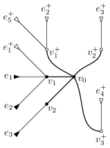
Figure 1. A picture of a stable scaled tree. Its base has three vertices $v_{0}$, $v_{1}$, and $v_{2}$. The vertices $v_{1}^{+}$, $v_{2}^{+}$, and $v_{3}^{+}$ are not in the base. We declare that the root $v_{0}$ has scale $\infty$ and other vertices have scale $1$. The three black incoming arrows are semi-infinite edges in the base and the other white incoming arrows are semi-infinite edges not in the base. The ribbon tree structure of the base is induced from the way we draw the picture. This tree is a simple tree in the sense of Definition 2.18. This tree can model a stable affine vortex with one holomorphic disk component, two affine vortex components over ${\mathbb{H}}$, three affine vortex components over ${\mathbb{C}}$, three boundary marked points, and five interior marked points.

Definition 2.10.

Let $(\Gamma,{\mathfrak{s}})$ be a scaled tree. A marked scaled curve of type $(\Gamma,{\mathfrak{s}})$ is a collection

$${\mathcal{C}}=\left((\Sigma_{\alpha},\sigma_{\alpha},f_{\alpha})_{v_{\alpha}\in V_{\Gamma}},\ (z_{e})_{e\in E_{\Gamma}}\right)$$

where

• For each $v_{\alpha}\in V_{\underline{\smash{\Gamma}}{}}$ resp. $V_{\Gamma^{\rm sup}}$, $\Sigma_{\alpha}$ is a bordered resp. closed Riemann surface, $\sigma_{\alpha}\in\Omega^{2}(\Sigma_{\alpha})\cup\{\infty\}$, and $f_{\alpha}:\Sigma_{\alpha}\cong{\mathbb{H}}$ resp. $f_{\alpha}:\Sigma_{\alpha}\cong{\mathbb{C}}$ is a biholomorphism such that ${\mathfrak{s}}(v_{\alpha})f_{\alpha}^{*}dsdt=\sigma_{\alpha}$.

• For each $e\in E_{\Gamma}$, $z_{e}\in\Sigma_{\alpha(e)}$.

They satisfy the following conditions.

1. If $e\in E_{\underline{\smash{\Gamma}}{}}$, then $z_{e}\in\partial\Sigma_{\alpha}$; otherwise $z_{e}\in{\rm Int}\Sigma_{\alpha}$.

2. For each vertex $v_{\alpha}$, the collection of points defining the set

   $$Z_{\alpha}:=\{z_{e}\ |\ \alpha(e)=\alpha\}$$

   are distinct.

The marked scaled curve is stable if the tree $(\Gamma,{\mathfrak{s}})$ is stable.

Definition 2.11.

Let ${\mathcal{C}}=((\Sigma_{\alpha},\sigma_{\alpha},f_{\alpha}),(z_{e}))$ and ${\mathcal{C}}^{\prime}=((\Sigma_{\alpha}^{\prime},\sigma_{\alpha}^{\prime},f_{\alpha}^{\prime}),(z_{e}^{\prime}))$ be two marked scaled curve of type $\Gamma$. An isomorphism from ${\mathcal{C}}$ to ${\mathcal{C}}^{\prime}$ is a collection of biholomorphism

$$(\varphi_{\alpha}:(\overline{\Sigma}_{\alpha},\infty)\to(\overline{\Sigma}_{\alpha},\infty))$$

satisfying the following conditions

1. For each $v_{\alpha}\in V_{\Gamma}$, one has $f_{\alpha}=f_{\alpha}^{\prime}\circ\varphi_{\alpha}$.

2. For each $e\in E_{\Gamma}$, one has $\varphi_{\alpha(e)}(z_{e})=z_{e}^{\prime}$.

We say a marked scaled curve is smooth if the underlying tree $\Gamma$ has a single vertex $v_{0}$ with ${\mathfrak{s}}(v_{0})=1$. In this case we can represent a smooth marked scaled curve as

$$\big{(}({\mathbb{H}},ds\wedge dt,{\rm Id}),{\bm{z}}=(z_{e})_{e\in E_{\Gamma}^{\infty}}\big{)}$$

where $(z_{e})_{e\in E_{\Gamma}^{\infty}}$ is a configuration of distinct points in the upper half plane. Since semi-infinite edges are labeled by integers, the point configuration is also denoted by

$${\bm{z}}=(z_{1},\ldots,z_{l};z_{1}^{+},\ldots,z_{l^{+}}^{+})$$

where $l=\#E_{\underline{\smash{\Gamma}}{}}^{\infty}$ and $l^{+}=\#(E_{\Gamma}^{\infty}\smallsetminus E_{\underline{\smash{\Gamma}}{}}^{\infty})$. By Definition 2.11, two smooth marked scaled curves with $l$ boundary markings and $l^{+}$ interior markings are isomorphic if the corresponding point configurations differ by a real translation in the upper half plane.

It is easy to see that the automorphism group of a marked scaled curve is finite if and only if it is stable. In this case the automorphism group is actually trivial (as we are in genus zero). For each stable scaled tree $\Gamma$, let ${\mathcal{M}}_{\Gamma}$ be the set of isomorphism classes of marked scaled curves of type $\Gamma$. When $\Gamma$ is stable has a single vertex $v_{0}$ with ${\mathfrak{s}}(v_{0})=1$ (as described above), then the moduli space ${\mathcal{M}}_{\Gamma}$ can be identified with the space of point configurations modulo translation, and hence is a manifold. For a general stable $\Gamma$, the moduli space ${\mathcal{M}}_{\Gamma}$ has a topology induced from the topology of the space of configurations of points on different components.

Denote by ${\rm Tree}(l,l^{+})$ the set of isomorphism classes of scaled trees with $l$ boundary semi-infinite edges and $l^{+}$ interior semi-infinite edges. By abuse of language, we regard each element of ${\rm Tree}(l,l^{+})$ as a tree rather than an isomorphism class. Let ${\rm Tree}^{s}(l,l^{+})\subset{\rm Tree}(l,l^{+})$ be the subset of stable trees. Then define

$$\overline{\mathcal{M}}_{l,l^{+}}=\bigsqcup_{\Gamma\in{\rm Tree}^{s}(l,l^{+})}{\mathcal{M}}_{\Gamma}.$$

A natural topology can be defined on $\overline{\mathcal{M}}_{l,l^{+}}$ stratified by ${\mathcal{M}}_{\Gamma}$. By the work of [10] the moduli space $\overline{\mathcal{M}}_{l,l^{+}}$ has the topology of a CW complex. We do not explore the detailed structure of this moduli space in general, though the structure near codimension one strata will be discussed later.

2.3. Moduli spaces of stable affine vortices

Now we describe the Gromov–Uhlenbeck compactification of the moduli space of affine vortices. For affine vortices over ${\mathbb{C}}$, such a compactification was firstly given by Ziltener [35, 37].

We first define the notion of stable vortices with respect to a fixed almost complex structure $J$. Later we will allow domain-dependent almost complex structures. Let $I$ be the induced almost complex structure on the symplectic quotient $X$.

Definition 2.12.

Let $\Gamma$ be a scaled tree. A stable affine vortex of type $\Gamma$ is a collection

$${\mathcal{V}}=({\mathcal{C}},({\bm{v}}_{\alpha})_{v_{\alpha}\in V_{\Gamma}})=\Big{(}(\Sigma_{\alpha},\sigma_{\alpha},f_{\alpha})_{v_{\alpha}\in V_{\Gamma}},(z_{e})_{e\in E_{\Gamma}},({\bm{v}}_{\alpha})_{v_{\alpha}\in V_{\Gamma}}\Big{)}.$$

Here

• ${\mathcal{C}}=((\Sigma_{\alpha},\sigma_{\alpha},f_{\alpha})_{v_{\alpha}\in V_{\Gamma}},(z_{e})_{e\in E_{\Gamma}})$ is a marked scaled curve of type $\Gamma$.

• For each $v_{\alpha}\in V_{\Gamma}^{0}$, ${\bm{v}}_{\alpha}$ is a $K$-orbit of holomorphic maps $u_{\alpha}:\Sigma_{\alpha}\to V$ satisfying the boundary condition $u_{\alpha}(\partial\Sigma_{\alpha})\subset L_{V}$.

• For each $v_{\alpha}\in V_{\Gamma}^{1}$, ${\bm{v}}_{\alpha}$ is a gauge equivalence class of solutions to (2.1) for volume form $\sigma_{\alpha}$ with boundary condition (2.2) (${\bm{v}}_{\alpha}$ is identified via $f_{\alpha}$ with a gauge equivalence class of affine vortices over ${\mathbb{C}}$ or ${\mathbb{H}}$).

• For each $v_{\alpha}\in V_{\Gamma}^{\infty}$, ${\bm{v}}_{\alpha}$ is an $I$-holomorphic map $\bar{u}_{\alpha}:\Sigma_{\alpha}\to X$ satisfying the boundary condition $\bar{u}_{\alpha}(\partial\Sigma_{\alpha})\subset L$.

They satisfy the following conditions.

1. (Matching condition) For each finite edge $e\in E_{\Gamma}^{-}$ connecting $v_{\beta}$ and $v_{\alpha(e)}$, the evaluation of ${\bm{v}}_{\beta}$ at infinity is equal to the evaluation of ${\bm{v}}_{\alpha(e)}$ at $z_{e}$.

2. (Stability condition) For each unstable vertex $v_{\alpha}$, the energy of ${\bm{v}}_{\alpha}$ is positive.

Convention 2.13.

We often use the same type of notations (i.e. ${\bm{v}}_{\alpha}$) denote different types of components. By abuse of notation, we also use ${\bm{v}}_{\alpha}=(u_{\alpha},\phi_{\alpha},\psi_{\alpha})$ to denote an actual gauged map, not its gauge equivalence class.

Definition 2.14.

Let ${\mathcal{V}}$, ${\mathcal{V}}^{\prime}$ be stable affine vortices of type $\Gamma$ where ${\mathcal{V}}$ is as described in Definition 2.12 and ${\mathcal{V}}^{\prime}=({\mathcal{C}}^{\prime},({\bm{v}}_{\alpha}^{\prime})_{v_{\alpha}\in V_{\Gamma}})$. An isomorphism from ${\mathcal{V}}$ to ${\mathcal{V}}^{\prime}$ is an isomorphism of marked scaled curves ${\bm{\varphi}}=(\varphi_{\alpha})_{v_{\alpha}\in V_{\Gamma}}$ from ${\mathcal{C}}$ to ${\mathcal{C}}^{\prime}$ such that

1. For each $v_{\alpha}\in V_{\Gamma}^{0}$, ${\bm{v}}_{\alpha}={\bm{v}}_{\alpha}^{\prime}\circ\varphi_{\alpha}$ as $K$-orbits of maps from $\Sigma_{\alpha}$ to $V$;

2. For each $v_{\alpha}\in V_{\Gamma}^{1}$, ${\bm{v}}_{\alpha}={\bm{v}}_{\alpha}^{\prime}\circ\varphi_{\alpha}$ as gauge equivalence classes of gauged maps;

3. For each $v_{\alpha}\in V_{\Gamma}^{\infty}$, ${\bm{v}}_{\alpha}={\bm{v}}_{\alpha}^{\prime}\circ\varphi_{\alpha}$ as maps from $\Sigma_{\alpha}$ to $X$.

Now we define the notion of sequential convergence of affine vortices towards stable affine vortices. For affine vortices over ${\mathbb{C}}$, this is defined by Ziltener [37, 35]. So we only describe the case for affine vortices over ${\mathbb{H}}$. We only state the definition for the case when elements of the sequence have smooth domains but it is standard to extend the following definition to the most general situation.

Definition 2.15.

Let

$${\mathcal{V}}_{k}=({\mathcal{C}}_{k},{\bm{v}}_{k})=((\Sigma_{k},\sigma_{k},f_{k}),(z_{k,e}),(u_{k},\phi_{k},\psi_{k}))$$

be a sequence of stable affine vortices with smooth domains $\Sigma_{k}\cong{\mathbb{H}}$, $l$ boundary marked points and $l^{+}$ interior marked points, and let

$${\mathcal{V}}=({\mathcal{C}},({\bm{v}}_{\alpha})_{v_{\alpha}\in V_{\Gamma}})$$

be a stable affine vortex of type $\Gamma\in{\rm Tree}(l,l^{+})$ as described in Definition 2.12. We say that ${\mathcal{V}}_{k}$ converges (modulo gauge transformation and translation) to ${\mathcal{V}}$ if there exist a collection of sequences of Möbius transformations

$$\varphi_{k,\alpha}:({\mathbb{C}},\infty)\to({\mathbb{C}},\infty)$$

satisfying the following conditions.

1. For each $v_{\alpha}\in V_{\underline{\smash{\Gamma}}{}}$, $\varphi_{k,\alpha}$ is real, namely $\varphi_{k,\alpha}$ maps ${\mathbb{H}}$ to ${\mathbb{H}}$.

2. For each $v_{\alpha}\in V_{\Gamma}^{1}$, $\varphi_{k,\alpha}$ is a translation, namely $\varphi_{k,\alpha}(z)=z+t_{k,\alpha}$ for some $t_{k,\alpha}\in{\mathbb{C}}$.

3. For each semi-infinite edge $e\in E_{\Gamma}^{\infty}$, there holds

   $$\lim_{k\to\infty}f_{\alpha(e)}^{-1}\varphi_{k,\alpha}^{-1}(f_{k}(z_{k,e}))=z_{e}\in\Sigma_{\alpha(e)}.$$

   For each finite edge $e\in E_{\Gamma}^{-}$ connecting $v_{\alpha}$ and $v_{\beta}$ (where $v_{\beta}$ is closer to the root), there holds

   $$f_{\beta}^{-1}\circ\varphi_{k,\beta}^{-1}\circ\varphi_{k,\alpha}\circ f_{\alpha}\xrightarrow[k\to\infty]{C^{\infty}_{\rm loc}(\Sigma_{\alpha})}z_{e}\in\Sigma_{\beta}.$$

4. For each $v_{\alpha}\in V_{\Gamma}^{0}\cup V_{\Gamma}^{1}$, the sequence ${\bm{v}}_{k}\circ(f_{k}^{-1}\circ\varphi_{k,\alpha}\circ f_{\alpha})$ converges modulo gauge transformations to ${\bm{v}}_{\alpha}$.

5. For each $v_{\alpha}\in V_{\Gamma}^{\infty}$, there holds

   $$\mu(u_{k}\circ(f_{k}^{-1}\circ\varphi_{k,\alpha}\circ f_{\alpha}))\xrightarrow[k\to\infty]{C^{0}_{\rm loc}(\Sigma_{\alpha})}0.$$

   Moreover, there is a smooth map $u_{\alpha}:\Sigma_{\alpha}\to\mu^{-1}(0)$ whose projection to $X$ is the holomorphic map $\bar{u}_{\alpha}:\Sigma_{\alpha}\to X$ such that

   $$u_{k}\circ\varphi_{k,\alpha}\xrightarrow[k\to\infty]{C^{0}_{\rm loc}(\Sigma_{\alpha})}u_{\alpha}$$

6. There is no energy lost, namely,

   $$\lim_{k\to\infty}E({\bm{v}}_{k})=E({\mathcal{C}}):=\sum_{v_{\alpha}\in V_{\Gamma}}E({\bm{v}}_{\alpha}).$$

2.4. Families of almost complex structures

We would like to allow almost complex structures to be domain-dependent and depend on the domain moduli. This is the perturbation schemed used in [31]. We want the almost complex structures to be close to a base almost complex structure $J_{V}$. It is a $K$-invariant, $\omega_{V}$-compatible almost complex structure on $V$. We also require that $L_{V}$ is totally real with respect to $J_{V}$. Then $\omega_{V}$ and $J_{V}$ determine a Riemannian metric

$$g_{V}(\cdot,\cdot):=\omega_{V}(\cdot,J_{V}\cdot).$$

We would like the domain dependent almost complex structure to respect certain splittings of the tangent bundle. Let

$$(TV)_{K}\subset TV$$

be the set of infinitesimal $K$-actions. Define

$$(TV)_{G}:=(TV)_{K}\oplus J_{V}(TV)_{K}\subset TV$$

which is formally the set of “infinitesimal $G$-actions. By Hypothesis 2.1, $(TV)_{G}$ is a subbundle of $TV$ near $\mu^{-1}(0)$. It is easy to to see that the orthogonal complement

$$((TV)_{G})_{g_{V}}^{\bot}\subset TV$$

with respect to the metric $g_{V}$ is tangent to $\mu^{-1}(0)$. Moreover, if $\pi_{X}:\mu^{-1}(0)\to X$ is the projection, then there is a $K$-equivariant isomorphism

$$((TV)_{G})_{g_{V}}^{\bot}|_{\mu^{-1}(0)}\cong\pi_{X}^{*}TX.$$ (2.6)

Now we describe the type of domain-dependent almost complex structures we will use. Fix a pair of integers $(l,l^{+})$. There is a universal curve

$$\overline{\mathcal{U}}_{l,l^{+}}\to\overline{\mathcal{M}}_{l,l^{+}}$$

whose total space is $\overline{\mathcal{U}}_{l,l^{+}}\cong\overline{\mathcal{M}}_{l,l^{+}+1}$ and the projection $\overline{\mathcal{U}}_{l,l^{+}}\to\overline{\mathcal{M}}_{l,l^{+}}$ is forgetting the last interior marking. The fibre of the universal curve at a point $p\in\overline{\mathcal{M}}_{l,l^{+}}$ can be canonically identified with a stable marked scaled curve (up to isomorphism) representing the point $p$. The universal curve has the structure of smooth manifold with certain polyhedral corners (see the main result of [10] for the case $l=0$ or $l^{+}=0$) which allows one to have a notion of smoothness. There is a closed subset $\overline{\mathcal{U}}_{l,l^{+}}^{\rm node}\subset\overline{\mathcal{U}}_{l,l^{+}}$ corresponding to nodal points. There is also a closed subset $\overline{\mathcal{U}}_{l,l^{+}}^{\rm boundary}\subset\overline{\mathcal{U}}_{l,l^{+}}$ corresponding to boundary points. More generally, for each stable scaled tree $\Gamma\in{\rm Tree}^{s}(l,l^{+})$, denote by

$${\mathcal{U}}_{\Gamma}\subset\overline{\mathcal{U}}_{l,l^{+}}$$

the preimage of ${\mathcal{M}}_{\Gamma}\subset\overline{\mathcal{M}}_{l,l^{+}}$ under the projection $\overline{\mathcal{U}}_{l,l^{+}}\to\overline{\mathcal{M}}_{l,l^{+}}$. There is a subset

$${\mathcal{U}}_{\Gamma}^{\infty}\subset{\mathcal{U}}_{\Gamma}$$

corresponding to points on vertices in $V_{\Gamma}^{\infty}$.

Definition 2.16.

A family of domain-independent almost complex structures is a smooth map $J:\overline{\mathcal{U}}_{l,l^{+}}\to{\mathcal{J}}_{\rm tame}(V)$ where ${\mathcal{J}}_{\rm tame}(V)$ is the space of $K$-invariant $\omega_{V}$-tamed almost complex structures on $V$ satisfying the following conditions.

1. $J=J_{V}$ in a neighborhood of $\overline{\mathcal{U}}{}_{l,l^{+}}^{\rm node}\cup\overline{\mathcal{U}}{}_{l,l^{+}}^{\rm boundary}$.

2. For each stable tree $\Gamma\in{\rm Tree}^{s}(l,l^{+})$, the restriction of $J$ to ${\mathcal{U}}{}_{\Gamma}^{\infty}\times\mu^{-1}(0)$ preserves the subbundle $((TV)_{G})_{g_{V}}^{\bot}|_{\mu^{-1}(0)}$.

From now on we fix a family of domain-dependent almost complex structures. For each (not necessarily stable) scaled tree $\Gamma\in{\rm Tree}(l,l^{+})$ and a marked scaled curve ${\mathcal{C}}$ of type $\Gamma$, the family induces a domain-dependent almost complex structure $J_{\alpha}:\Sigma_{\alpha}\to{\mathcal{J}}_{\rm tame}(V)$ on each component $\Sigma_{\alpha}\subset{\mathcal{C}}$; if $v_{\alpha}\in V_{\Gamma}^{\infty}$ then via the isomorphism (2.6) $J_{\alpha}$ induces a map

$$I_{\alpha}:\Sigma_{\alpha}\to{\mathcal{J}}_{\rm tame}(X).$$

Denote by

$${\mathcal{M}}_{\Gamma}(V,L_{V})$$

the moduli space of isomorphism classes of stable affine instantons of type $\Gamma$ with respect to the family of almost complex structures. Moreover, define

$$\overline{\mathcal{M}}_{l,l^{+}}(V,L_{V}):=\bigsqcup_{\Gamma}{\mathcal{M}}_{\Gamma}(V,L_{V})$$

where the union is taken over all (not necessarily stable) scaled trees $\Gamma\in{\rm Tree}(l,l^{+})$. One can define a notion of sequential convergence by generalizing Definition 2.15. The notion of sequential convergence then induces a topology on $\overline{\mathcal{M}}_{l,l^{+}}(V,L_{V})$. Moreover, for each real number $E>0$, let

$$\overline{\mathcal{M}}_{l,l^{+}}^{\leq E}(V,L_{V})\subset\overline{\mathcal{M}}_{l,l^{+}}(V,L_{V})$$

be the subset of stable affine vortices whose energy (computed using a fixed Riemannian metric on $V$) is at most $E$.

We recall the compactness theorem for the moduli space of stable affine vortices. The case of affine vortices over ${\mathbb{C}}$ was proved by Ziltener [37, 35]. The case of affine vortices over ${\mathbb{H}}$, though not explicitly stated and proved, can be produced from [25].

Theorem 2.17 (Compactness theorem).

Fix $l,l^{+}\geq 0$ with $l+l^{+}\geq 1$ and a family of domain-dependent almost complex structures $J:\overline{\mathcal{U}}_{l,l^{+}}\to{\mathcal{J}}_{\rm tame}(V)$. For any $E>0$, the subset $\overline{\mathcal{M}}_{l,l^{+}}^{\leq E}(V,L_{V})$ is sequentially compact.

2.5. Codimension one degeneration

The goal of this paper is to provide a local model for the compactified moduli space near a point in a codimension one stratum. In this subsection, we first describe the local model of the domain moduli for such a stratum.

Definition 2.18.

A scaled tree $\Gamma$ is called simple if $V_{\Gamma}^{\infty}=\{v_{0}\}$ and $V_{\Gamma}^{1}=V_{\Gamma}\smallsetminus\{v_{0}\}$.

From now on we fix a simple stable scaled tree $\Gamma$ with $l$ boundary semi-infinite edges, $l^{+}$ interior semi-infinite edges, with

$$\ \#V_{\underline{\smash{\Gamma}}{}}^{1}=m,\ \ \#V_{\Gamma^{\rm sup}}^{1}=m^{+}.$$

From now on throughout this paper, we order and label the finite edges by integers as

$$e_{1},\ldots,e_{m};\ e_{1}^{+},\ldots,e_{m^{+}}^{+}.$$

Then the corresponding vertices $v_{\alpha}\in V_{\Gamma}^{1}$ are denoted by $v_{1},\ldots,v_{m};v_{1}^{+},\ldots,v_{m^{+}}^{+}$. We also label them in a different way as

$$v_{i},\ i=1,\ldots,m+m^{+},\ {\rm where}\ v_{m+i}:=v_{i}^{+}.$$

For each $e\in E_{\Gamma}^{\infty}$, let $i(e)$ be the integer labeling the vertex $v_{i(e)}$ containing $e$.

We would like to see the local structure of $\overline{\mathcal{M}}_{l,l^{+}}$ near a point $p\in{\mathcal{M}}_{\Gamma}$. First, it is easy to see that ${\mathcal{M}}_{\Gamma}$ is a smooth manifold. Indeed, for $v_{i}\in V_{\Gamma}^{1}$, let $\Gamma_{i}$ be the scaled tree with only one vertex $v_{i}$ (with scale $1$) whose semi-infinite edges are all semi-infinite edges in $\Gamma$ attached to $v_{1}$. Then there is a canonical homeomorphism

$${\mathcal{M}}_{\Gamma}\cong{\mathcal{M}}_{m+1,m^{+}}^{\rm disk}\times\prod_{i=1}^{m+m^{+}}{\mathcal{M}}_{\Gamma_{i}}.$$

Here ${\mathcal{M}}_{m+1,m^{+}}^{\rm disk}$ is the moduli space of marked disks with $m+1$ boundary markings and $m^{+}$ interior markings. A point $p\in{\mathcal{M}}_{\Gamma}$ can be written as $(p_{0},\ldots,p_{m+m^{+}})$. Denote

$$\ W_{i}:=T_{p_{i}}{\mathcal{M}}_{\Gamma_{i}},\ i=1,\ldots,m+m^{+};\ \ W_{0}:=T_{p_{0}}{\mathcal{M}}_{m+1,m^{+}}^{\rm disk}\cong{\mathbb{R}}^{m+2m^{+}-2}.$$

We fix the following data.

1. Metrics on $W_{i}$ for $i=0,\ldots,m+m^{+}$. For $\tau>0$ let $W_{i}^{\tau}\subset W_{i}$ be the radius $\tau$ ball centered at the origin.

2. For $i=1,\ldots,m+m^{+}$, a configuration of points ${\bm{z}}_{i}=(z_{e})_{i(e)=i}$ in ${\mathbb{C}}$ or ${\mathbb{H}}$ representing the point $p_{i}\in{\mathcal{M}}_{\Gamma_{i}}$.

3. A configuration of points ${\bm{z}}_{0}=(z_{1},\ldots,z_{m};z_{1}^{+},\ldots,z_{m^{+}}^{+})$ in ${\mathbb{H}}$ such that the marked disk $({\mathbb{H}}\cup\{\infty\};z_{1},\ldots,z_{m},\infty;z_{1}^{+},\ldots,z_{m^{+}}^{+})$ represents the point $p_{0}\in{\mathcal{M}}_{m+1,m^{+}}^{\rm disk}$.

4. A sufficiently small $\tau>0$ and for each $v_{i}\in V_{\Gamma}^{1}$, a family of configurations

   $${\bm{z}}_{i}({\bm{w}}_{i})=(z_{e}({\bm{w}}_{i}))_{i(e)=i}$$

   parametrized smoothly by ${\bm{w}}_{i}\in W_{i}^{\tau}$ such that the map

   $${\bm{w}}_{i}\mapsto[({\mathbb{A}}_{i},ds\wedge dt,{\rm Id}),{\bm{z}}_{i}({\bm{w}}_{i})]$$

   (where $[\cdot]$ means the isomorphism class of marked scaled curves) is a homeomorphism onto a neighborhood of $p_{i}$ in ${\mathcal{M}}_{\Gamma_{i}}$.

5. A smooth family of diffeomorphisms

   $$f_{{\bm{w}}_{0}}=s_{{\bm{w}}_{0}}+{\bm{i}}t_{{\bm{w}}_{0}}:{\mathbb{H}}\to{\mathbb{H}}$$ (2.7)

   such that the support of $df_{{\bm{w}}_{0}}-{\rm Id}$ is contained in a common compact subset which is disjoint from $z_{1},\ldots,z_{m};z_{1}^{+},\ldots,z_{m^{+}}^{+}$, and such that the map

   $$W_{0}^{\tau}\ni{\bm{w}}_{0}\mapsto p_{0}({\bm{w}}_{0})=[\Sigma_{{\bm{w}}_{0}};z_{1},\ldots,z_{m},\infty;z_{1}^{+},\ldots,z_{m^{+}}^{+}]$$

   is a homeomorphism onto a neighborhood of $p_{0}$ in ${\mathcal{M}}_{m+1,m^{+}}^{\rm disk}$. Here $\Sigma_{{\bm{w}}_{0}}$ is the bordered Riemann surface whose underlying surface is ${\mathbb{D}}\cong{\mathbb{H}}\cup\{\infty\}$ and whose complex structure is induced from the coordinate $s_{{\bm{w}}_{0}}+{\bm{i}}t_{{\bm{w}}_{0}}$. Equivalently, The diffeomorphism $z_{{\bm{w}}_{0}}$ gives a family of configurations

   $${\bm{z}}_{0}({\bm{w}}_{0}):=(z_{i}({\bm{w}}_{0}))_{i=1}^{m+m^{+}}=(z_{{\bm{w}}_{0}}(z_{i}))_{i=1}^{m+m^{+}}$$

   so that the marked disk (with the standard complex structure)

   $$({\mathbb{H}}\cup\{\infty\};z_{1}({\bm{w}}_{0}),\ldots,z_{m}({\bm{w}}_{0}),\infty;z_{1}^{+}({\bm{w}}_{0}),\ldots,z_{m^{+}}^{+}({\bm{w}}_{0}))$$

   represents the same point $p_{0}({\bm{w}}_{0})\in{\mathcal{M}}_{m+1,m^{+}}^{\rm disk}$.

Denote

$$\ W_{\rm def}:=\bigoplus_{v_{\alpha}\in V_{\Gamma}}W_{\alpha},\ \ W_{\rm def}^{\tau}:=\prod_{v_{\alpha}\in V_{\Gamma}}W_{\alpha}^{\tau}.$$

Elements of $W_{\rm def}$, called deformation parameters, are denoted by ${\bm{w}}=({\bm{w}}_{\alpha})_{v_{\alpha}\in V_{\Gamma}}$. The data we just fixed induce a family of marked stable scaled curves of type $\Gamma$, denoted by

$${\mathcal{C}}_{0,{\bm{w}}},\ {\bm{w}}\in W_{\rm def}^{\tau}.$$

We would like to turn on the gluing parameter and obtain a local model of the moduli $\overline{\mathcal{M}}_{l,l^{+}}$. Denote

$$z_{i,\epsilon}({\bm{w}}_{0}):=\frac{z_{i}({\bm{w}}_{0})}{\epsilon},\ i=1,\ldots,m+m^{+}$$

and for each $e\in E_{\Gamma}^{\infty}$, define

$$z_{e,\epsilon}({\bm{w}}):=z_{e}({\bm{w}}_{i(e)})+z_{i(e),\epsilon}({\bm{w}}_{0}).$$

This gives a family of configurations of points in ${\mathbb{H}}$. For $\tau>0$ small enough, define

$$\Phi_{p}:[0,\tau)\times W_{\rm def}^{\tau}\to\overline{\mathcal{M}}_{l,l^{+}},(\epsilon,{\bm{w}})\mapsto\left\{\begin{array}[]{cc}{[}{\mathcal{C}}_{0,{\bm{w}}}{]},&\ \epsilon=0,\\ {[}{\mathcal{C}}_{\epsilon,{\bm{w}}}{]}:={[}({\mathbb{H}},ds\wedge dt,{\rm Id});(z_{e,\epsilon}({\bm{w}}))_{e\in E_{\Gamma}^{\infty}}{]},&\ \epsilon\neq 0.\end{array}\right.$$ (2.8)

Then one has

Lemma 2.19.

For $\tau$ small enough, the map $\Phi_{p}$ is a homeomorphism onto an open neighborhood of $p$ in $\overline{\mathcal{M}}_{l,l^{+}}$.

Using the domain local model given above the family of domain-dependent almost complex structures can be regarded as depending on the gluing parameter and the deformation parameter. More precisely, for any stable marked scaled curve ${\mathcal{C}}$ representing a point in the image of $\Phi_{p}$, we can identify ${\mathcal{C}}$ with a certain ${\mathcal{C}}_{\epsilon,{\bm{w}}}$. Then $J:\overline{\mathcal{U}}_{l,l^{+}}\to{\mathcal{J}}_{\rm tame}(V)$ induces a domain-dependent almost complex structure

$$J_{\epsilon,{\bm{w}}}:{\mathcal{C}}\cong{\mathcal{C}}_{\epsilon,{\bm{w}}}\to{\mathcal{J}}_{\rm tame}(V).$$

For the purpose of constructing the gluing map, we slightly modify the local model given above. The idea is to fix the positions of the nodal points while varying the complex structure on the disk component away from the nodal points. Denote

$$s_{\epsilon}:{\mathbb{H}}\to{\mathbb{H}},\ z\mapsto\epsilon z$$ (2.9)

and call it the $\epsilon$-rescaling. Then let $\Sigma_{\epsilon,{\bm{w}}}$ be bordered Riemann surface whose underlying surface is ${\mathbb{H}}$ and whose complex structure is induced from the coordinate

$$f_{\epsilon,{\bm{w}}}=s_{\epsilon,{\bm{w}}}+{\bm{i}}t_{\epsilon,{\bm{w}}}:=s_{\epsilon}^{-1}\circ f_{{\bm{w}}_{0}}\circ s_{\epsilon}.$$

Here $f_{{\bm{w}}_{0}}:{\mathbb{H}}\to{\mathbb{H}}$ is the family of diffeomorphisms (2.7). Furthermore, define

$$\sigma_{\epsilon,{\bm{w}}}^{\prime}:=ds_{\epsilon,{\bm{w}}}\wedge dt_{\epsilon,{\bm{w}}}$$

which is a volume form on $\Sigma_{\epsilon,{\bm{w}}}$. Define

$${\mathcal{C}}_{\epsilon,{\bm{w}}}^{\prime}:=\big{(}(\Sigma_{\epsilon,{\bm{w}}},\sigma_{\epsilon,{\bm{w}}}^{\prime},f_{\epsilon,{\bm{w}}});{\bm{z}}_{\epsilon,{\bm{w}}}^{\prime}\big{)}$$

where ${\bm{z}}_{\epsilon,{\bm{w}}}^{\prime}$ is the configuration

$$\Big{(}z_{e,{\bm{w}}}^{\prime}=z_{e}({\bm{w}}_{i(e)})+\frac{z_{i}}{\epsilon}\Big{)}_{e\in E_{\Gamma}^{\infty}}.$$

Then ${\mathcal{C}}_{\epsilon,{\bm{w}}}^{\prime}$ also parametrizes a neighborhood of $p$ in $\overline{\mathcal{M}}_{l,l^{+}}$ and gives the same map as $\Phi_{p}$ (see 2.8) and the family of biholomorphisms

$$f_{\epsilon,{\bm{w}}}:{\mathcal{C}}_{\epsilon,{\bm{w}}}^{\prime}\cong{\mathcal{C}}_{\epsilon,{\bm{w}}}$$

intertwines the volume form $\sigma_{\epsilon,{\bm{w}}}^{\prime}$ resp. marked points ${\bm{z}}_{\epsilon,{\bm{w}}}^{\prime}$ on the former with the standard volume form $ds\wedge dt$ resp. marked points ${\bm{z}}_{\epsilon,{\bm{w}}}$ on the latter.

Using this new family the vortex equation (2.3) takes a slightly different form. The family of almost complex structures $J$ induces a domain-dependent almost complex structure $J_{\epsilon,{\bm{w}}}:\Sigma_{\epsilon,{\bm{w}}}\to{\mathcal{J}}_{\rm tame}(V)$. Then (2.3) is equivalent to the following

$$\begin{split}\partial_{s_{\epsilon,{\bm{w}}}}u+{\mathcal{X}}_{\phi}(u)+J_{\epsilon,{\bm{w}}}(\partial_{t_{\epsilon,{\bm{w}}}}u+{\mathcal{X}}_{\psi}(u))=&0,\\ \partial_{s_{\epsilon,{\bm{w}}}}\psi-\partial_{t_{\epsilon,{\bm{w}}}}\phi+[\phi,\psi]+\mu(u)=&0.\end{split}$$ (2.10)

3. The Main Theorem

In this section we state the main theorem of this paper, under a precise version of the transversality assumption.

3.1. Local model of affine vortices

We recall the main result of [23] which provides the local model of affine vortices.

Since the domain of affine vortices is noncompact, Fredholm theory requires certain Sobolev completions of the domains and codomains of the linearized operator. The particular choices of these norms reflects the complicated asymptotic behavior of affine vortices. Choose a smooth weight function $\rho_{\mathbb{A}}:{\mathbb{A}}\to[1,+\infty)$ such that outside the unit disk, $\rho_{\mathbb{A}}(z)=|z|^{2}$. Let $\delta\in{\mathbb{R}}$ be a real parameter. For $f\in L{}^{p}_{\rm loc}({\mathbb{A}})$ define

$$\|f\|_{L^{p,\delta}}:=\left[\int_{\mathbb{A}}|f(z)|^{p}(\rho_{\mathbb{A}}(z))^{\frac{p\delta}{2}}dsdt\right]^{\frac{1}{p}}.$$

We can generalize this norm to sections of certain Euclidean bundle $E$ over certain subset of ${\mathbb{A}}$. On the other hand, we will use to different norms to complete the space of functions with local $W^{1,p}$-regularity. Define

$$\|f\|_{L^{1,p,\delta}_{H}}:=\|f\|_{L^{\infty}}+\|\nabla f\|_{L^{p,\delta}}$$ (3.1)

and

$$\|f\|_{L^{1,p,\delta}_{G}}:=\|f\|_{L^{p,\delta}}+\|\nabla f\|_{L^{p,\delta}}.$$ (3.2)

The completions of the domains and codomains of the linearized operators are modelled on the above Sobolev spaces. We first introduce a few new notations. Let ${\bm{v}}=(u,\phi,\psi)$ be an affine vortex. Denote the connection form by

$$a=\phi ds+\psi dt\in\Omega^{1}({\mathbb{A}},{\mathfrak{k}}).$$

Introduce a covariant derivative of sections $\xi$ of $u^{*}TV$ resp. ${\mathfrak{k}}$-valued functions $f$ on ${\mathbb{A}}$ by

$$\begin{split}\nabla_{s}^{a}\xi=\nabla_{s}\xi+\nabla_{\xi}{\mathcal{X}}_{\phi}\ &{\rm resp.}\ \nabla_{s}^{a}f=\partial_{s}f+[\phi,f],\\ \nabla_{t}^{a}\xi=\nabla_{t}\xi+\nabla_{\xi}{\mathcal{X}}_{\psi}\ &{\rm resp.}\ \nabla_{t}^{a}f=\partial_{t}f+[\psi,f].\end{split}$$

Then for ${\bm{\xi}}=(\xi,\eta,\zeta)\in{\mathit{\Gamma}}(u^{*}TV\oplus{\mathfrak{k}}\oplus{\mathfrak{k}})$, define the norm

$$\|{\bm{\xi}}\|_{L^{1,p,\delta}_{m}}:=\|\xi\|_{L^{\infty}}+\|\nabla^{a}{\bm{\xi}}\|_{L^{p,\delta}}+\|d\mu(u)(\xi)\|_{L^{p,\delta}}+\|d\mu(u)(J_{V}\xi)\|_{L^{p,\delta}}+\|\eta\|_{L^{p,\delta}}+\|\zeta\|_{L^{p,\delta}}.$$ (3.3)

Here $m$ stands for “mixed.” It was proved in [37] for ${\mathbb{A}}={\mathbb{C}}$ and in [23] for ${\mathbb{A}}={\mathbb{H}}$ that the above norm is complete. We define

$$\hat{\mathcal{B}}_{\bm{v}}:=\Big{\{}{\bm{\xi}}=(\xi,\eta,\zeta)\in W^{1,p}_{\rm loc}({\mathbb{A}},u^{*}TV\oplus{\mathfrak{k}}\oplus{\mathfrak{k}})\ |\ \|{\bm{\xi}}\|_{L^{1,p,\delta}_{m}}<\infty,\ \xi|_{\partial{\mathbb{H}}}\subset TL_{V},\ \zeta|_{\partial{\mathbb{H}}}=0\Big{\}}.$$

The “Coulomb slice” is the subspace

$${\mathcal{B}}_{\bm{v}}:=\Big{\{}{\bm{\xi}}=(\xi,\eta,\zeta)\in\hat{\mathcal{B}}_{\bm{v}}\ |\ \partial_{s}\eta+[\phi,\eta]+\partial_{t}\zeta+[\psi,\zeta]+d\mu(u)(J_{V}\xi)=0\Big{\}}.$$ (3.4)

The main results of [23] can be summarized as follows.

Theorem 3.1 (Local model).

Fix $p>2$ and $\delta\in(1-\frac{2}{p},1)$. Let ${\mathbb{A}}$ be either ${\mathbb{C}}$ or ${\mathbb{H}}$. Let $(J_{z})$ be a smooth family of $K$-invariant almost complex structures on $V$ parametrized by $z\in{\mathbb{A}}$ such that $J_{z}=J_{V}$ for $|z|$ large. There is a Banach manifold ${\mathcal{B}}$, a Banach vector bundle ${\mathcal{E}}\to{\mathcal{B}}$, and a Fredholm section $F:{\mathcal{B}}\to{\mathcal{E}}$ satisfying the following conditions.

1. Each element of ${\mathcal{B}}$ is a gauge equivalence class of gauged maps from ${\mathbb{A}}$ to $V$ of regularity $W^{1,p}_{\rm loc}$ having limits at infinity as $K$-orbits. Moreover, the evaluation map at infinity ${\rm ev}_{\infty}:{\mathcal{B}}\to X$ is a smooth map.

2. The zero locus of $F$ consists of gauge equivalence classes of affine vortices over ${\mathbb{A}}$ and the natural map from $F^{-1}(0)$ to the moduli space of gauge equivalence classes of solutions to the vortex equation over ${\mathbb{A}}$ (for the almost complex structure $J_{z}$) is a homeomorphism between the Banach manifold topology on the former and the $C_{\rm loc}^{\infty}$ topology on the latter.

3. For each point ${\bm{p}}\in F^{-1}(0)$, choose a smooth representative ${\bm{v}}=(u,\phi,\psi)$, the tangent space of ${\mathcal{B}}$ at ${\bm{p}}$ is isomorphic to the space ${\mathcal{B}}_{\bm{v}}$ (see (3.4)), the fibre of ${\mathcal{E}}$ at ${\bm{p}}$ is isomorphic to ${\mathcal{E}}_{\bm{v}}\cong L^{p,\delta}({\mathbb{A}},u^{*}TV\oplus{\mathfrak{k}})$, and the linearization of $F$ at ${\bm{p}}$ is

   $$D_{\bm{p}}F({\bm{\xi}})=\left[\begin{array}[]{c}\nabla_{s}^{a}\xi+J_{z}\nabla_{t}^{a}\xi+(\nabla_{\xi}J_{z})(\partial_{t}u+{\mathcal{X}}_{\psi})+{\mathcal{X}}_{\eta}+J_{z}{\mathcal{X}}_{\zeta}\\ \nabla_{s}^{a}\zeta-\nabla_{t}^{a}\eta+d\mu(\xi)\end{array}\right].$$ (3.5)

4. The linearized operator $D_{\bm{p}}F:{\mathcal{B}}_{\bm{v}}\to{\mathcal{E}}_{\bm{v}}$ is a Fredholm operator.

3.2. Regular configurations

The existence of the gluing map relies on a certain transversality assumption. In this subsection we specify the transversality conditions. Let $\Gamma$ be a stable simple domain type (see Definition 2.18) with $l$ boundary semi-infinite edges and $l^{+}$ interior semi-infinite edges. Let $J:\overline{\mathcal{M}}_{l,l^{+}}\to{\mathcal{J}}_{\rm tame}(V)$ be a smooth family of domain-dependent almost complex structures. Let ${\mathcal{V}}=({\mathcal{C}},({\bm{v}}_{\alpha})_{v_{\alpha}\in V_{\Gamma}})$ be a stable affine vortex of type $\Gamma$ representing a point

$${\bm{p}}=[{\mathcal{V}}]\in{\mathcal{M}}_{\Gamma}(V,L_{V})\subset\overline{\mathcal{M}}_{l,l^{+}}(V,L_{V}).$$

We order vertices underlying affine vortices components in the same way as we label vertices of the tree in Subsection 2.5. Namely, let the components which are affine vortices over ${\mathbb{H}}$ be ${\bm{v}}_{1},\ldots,{\bm{v}}_{m}$ and the components which are affine vortices over ${\mathbb{C}}$ be ${\bm{v}}_{1}^{+},\ldots,{\bm{v}}_{m^{+}}^{+}$. We also introduce

$${\bm{v}}_{m+j}:={\bm{v}}_{j}^{+},\ j=1,\ldots,m^{+}$$

so ${\bm{v}}_{1},\ldots,{\bm{v}}_{m+m^{+}}$ are all the affine vortex components of ${\mathcal{V}}$. Up to isomorphism, we can assume that the domain of ${\bm{v}}_{i}$ be ${\mathbb{A}}_{i}$ which is either ${\mathbb{H}}$ or ${\mathbb{C}}$ with the standard structures.

For each vertex $v_{i}\in V_{\Gamma}^{1}$, let ${\mathcal{B}}_{i}$ be the Banach manifold parametrizing gauge equivalence classes of gauged maps defined over ${\mathbb{A}}_{i}$ and let ${\mathcal{E}}_{i}\to{\mathcal{B}}_{i}$ be the corresponding Banach vector bundle for a chosen $p\in(2,4)$ and $\delta=\delta_{p}=2-\frac{4}{p}$ (see Theorem 3.1). On the other hand, for the holomorphic disk component, there is a Banach manifold

$${\mathcal{B}}_{0}=\big{\{}\bar{u}_{0}^{\prime}\in W^{1,p}({\mathbb{D}}^{2},X)\ |\ \bar{u}_{0}^{\prime}(\partial{\mathbb{D}}^{2})\subset L\big{\}}.$$

There is a Banach vector bundle ${\mathcal{E}}_{0}\to{\mathcal{B}}_{0}$ whose fibre over a map $\bar{u}_{0}^{\prime}$ is

$${\mathcal{E}}_{0}|_{\bar{u}_{0}^{\prime}}=L^{p}({\mathbb{D}}^{2},\Lambda^{0,1}\otimes(\bar{u}_{0}^{\prime})^{*}TX).$$

Now we describe the local model for the singular configuration. Define

$${\mathcal{B}}_{\Gamma}^{\#}:={\mathcal{B}}_{0}\times\prod_{i=1}^{m+m^{+}}{\mathcal{B}}_{i}.$$

This is direct product of spaces of component-wise configurations whose values at nodal points may not match. Define

$${\mathcal{B}}_{\Gamma}:=\Big{\{}(\bar{u}_{0}^{\prime},{\bm{v}}_{1}^{\prime},\ldots,{\bm{v}}_{m+m^{+}}^{\prime})\in{\mathcal{M}}_{\Gamma}\times{\mathcal{B}}_{\Gamma}^{\#}\ |\ {\rm the\ ``matching\ condition"}\Big{\}}.$$ (3.6)

Here the matching condition means the following:

• (Matching condition) For each vertex $v_{i}\in V_{\Gamma}^{1}$, one has

  $${\bm{v}}_{i}^{\prime}(\infty)=\bar{u}_{0}^{\prime}(z_{i})$$

  as points in $X$ (if $v_{\alpha}\in V_{\Gamma^{\rm sup}}$) or $L$ (if $v_{\alpha}\in V_{\underline{\smash{\Gamma}}{}}$).

There is also the direct sum of Banach vector bundles. Denote

$${\mathcal{E}}_{\Gamma}^{\#}:={\mathcal{E}}_{0}\oplus\bigoplus_{i=1}^{m+m^{+}}{\mathcal{E}}_{i}\to{\mathcal{B}}_{\Gamma}^{\#}.$$

By pulling back and restriction one has the Banach vector bundle

$${\mathcal{E}}_{\Gamma}\to{\mathcal{B}}_{\Gamma}.$$

Then using the family of domain-dependent almost complex structure $J$ specified previously, using Theorem 3.1 and the standard facts about local models of holomorphic disks, the vortex equation and the holomorphic curve equation provide a Fredholm section

$${\mathcal{F}}_{\Gamma}:W_{\rm def}\times{\mathcal{B}}_{\Gamma}\to{\mathcal{E}}_{\Gamma}.$$

By Theorem 3.1, there is a natural homeomorphism

$${\mathcal{F}}_{\Gamma}^{-1}(0)\cong{\mathcal{M}}_{\Gamma}(V,L_{V}).$$

The linearization of ${\mathcal{F}}_{\Gamma}$ at point ${\bm{p}}\in{\mathcal{F}}_{\Gamma}^{-1}(0)$ (which is independent of how one locally trivializes the bundle ${\mathcal{E}}_{\Gamma}$) is a linear Fredholm operator

$$D_{\bm{p}}{\mathcal{F}}_{\Gamma}:W_{\rm def}\oplus T_{\bm{p}}{\mathcal{B}}_{\Gamma}\to{\mathcal{E}}_{\Gamma}|_{{\bm{p}}}.$$ (3.7)

Definition 3.2.

A point ${\bm{p}}\in{\mathcal{F}}_{\Gamma}^{-1}(0)$ is called regular if the linear operator $D_{\bm{p}}{\mathcal{F}}_{\Gamma}$ in (3.7) is surjective; the point ${\bm{p}}$ is called rigid if the index of $D_{\bm{p}}{\mathcal{F}}_{\Gamma}$ is zero.

Now we can state our main theorem.

Theorem 3.3.

Suppose $\Gamma$ is a simple stable scaled tree with $l$ boundary semi-infinite edges and $l^{+}$ interior semi-infinite edges. Given a regular and rigid point ${\bm{p}}\in{\mathcal{M}}_{\Gamma}(V,L_{V})$, there is an open neighborhood ${\mathcal{U}}\subset\overline{\mathcal{M}}_{l,l^{+}}(V,L_{V})$ of ${\bm{p}}$ which is homeomorphic to an interval $[0,\tau)$ where $0$ corresponds to ${\bm{p}}$.

Remark 3.4.

There are two reasons why we do not consider the case of having unstable components. If there are unstable components one just adds extra marked points to stabilize, which does not make an essential difference. On the other hand, in the case of using stabilizing divisors and domain dependent almost complex structures (which is the approach of [31]), there cannot be unstable components in a stable object.

Remark 3.5.

The construction of this paper extends without difficulty to the situation when $\Gamma$ is a stable simple scaled tree with empty base. In that case the gluing parameter is a complex number and all equations have no boundary condition.

4. Preparation

The proof of Theorem 3.3 is straightforward and resembles the gluing construction of holomorphic curves. However, because the singular configuration we start with mixes two different types of equations, and because the analysis of affine vortices is much more complicated than holomorphic curves, to prepare for the straightforward argument, one needs to adjust the standard gluing apparatus in many aspects. In this section we make various technical preparations. In Subsection 4.1 we specify a Riemannian metric allowing one to construct nearby gauged maps and a connection needed to linearize the vortex equation at a general gauged map. In Subsection 4.2 we recall the “augmented linearization” of the vortex equation which is convenient to use in the case when the equation has gauge symmetry. In Subsection 4.3 we fix the gauge for affine vortex components such that the affine vortices have good asymptotic behavior. In Subsection 4.4 we rewrite the linear theory of the holomorphic disk component, putting it into a setting closer to the affine vortex equation. In Subsection 4.5 and Subsection 4.6, we define an $\epsilon$-dependent family of singular configurations, define an $\epsilon$-dependent bounded operator $\hat{\mathcal{Q}}_{\Gamma,\epsilon}$ (playing the role as a right inverse of the linearization at the singular configuration), and show that the operator norm of $\hat{\mathcal{Q}}_{\Gamma,\epsilon}$ has a uniform upper bound.

4.1. Metric and connection

We will need a good metric on $V$ and will use its exponential map to identify small infinitesimal deformations with nearby gauged maps.

Lemma 4.1.

(cf. [25, Lemma 49]) There exists a $K$-invariant Riemannian metric $h_{V}$ on $V$ satisfying the following conditions.

1. The base almost complex structure $J_{V}$ is $h_{V}$-isometric along $L_{V}$.

2. $J_{V}(TL_{V})$ is orthogonal to $TL_{V}$ with respect to $h_{V}$.

3. $L_{V}$ and $\mu^{-1}(0)$ are totally geodesic with respect to $h_{V}$.

4. $T\mu^{-1}(0)$ is orthogonal to the distribution spanned by $J_{V}{\mathcal{X}}_{a}$ for all $a\in{\mathfrak{k}}$.

5. The subbundle $((TV)_{G})_{g_{V}}^{\bot}|_{\mu^{-1}(0)}\subset TV|_{\mu^{-1}(0)}$ (which is the orthogonal complement of $(TV)_{G}$ with respect to $g_{V}$) is also the orthogonal complement of $(TV)_{G}$ with respect to $h_{V}$.

Proof.

Recall that one has the $K$-equivariant decomposition

$$T\mu^{-1}(0)=((TV)_{G})_{g_{V}}^{\bot}|_{\mu^{-1}(0)}\oplus(TV)_{K}|_{\mu^{-1}(0)}.$$ (4.1)

Moreover one has a $K$-equivariant isomorphisms

$$\ ((TV)_{G})_{g_{V}}^{\bot}|_{\mu^{-1}(0)}\cong\pi_{X}^{*}TX,\ \ (TV)_{K}|_{\mu^{-1}(0)}\cong X\times{\mathfrak{k}}.$$ (4.2)

Here

$$\pi_{X}:\mu^{-1}(0)\to X=\mu^{-1}(0)/K$$

is the projection. By [6, Lemma A.3], there is a Riemannian metric $h_{X}$ on the symplectic quotient $X$ such that the quotient almost complex structure $J_{X}$ is isometric, $J_{X}(TL)$ is orthogonal to $TL$, and $L\subset X$ is totally geodesic. On the other hand, choose a $K$-invariant metric $h_{\mathfrak{k}}$ on the Lie algebra ${\mathfrak{k}}$. Then using the decomposition (4.1) and the isomorphisms (4.2), one takes the direct sum $\pi_{X}^{*}h_{X}\oplus h_{\mathfrak{k}}$ which is a Riemannian metric $h_{\mu^{-1}(0)}$ on $\mu^{-1}(0)$. In the proof of [25, Lemma 49] it was proved that $L_{V}$ is totally geodesic inside $\mu^{-1}(0)$.

Next we extend the metric $h_{\mu^{-1}(0)}$ to a metric in $V$. For a small $r>0$, let ${\mathfrak{k}}_{r}\subset{\mathfrak{k}}$ be the radius $r$ ball centered at the origin with respect to the metric $h_{\mathfrak{k}}$. Define a map

$$\iota:\mu^{-1}(0)\times{\mathfrak{k}}_{r}\to V,\ \ (x,\eta)\mapsto\exp_{x}(J_{V}{\mathcal{X}}_{\eta})$$

where $\exp$ is the exponential map of the metric $g_{V}$. Then the map $\iota$ is a $K$-equivariant open embedding ($K$ acts diagonally on $\mu^{-1}(0)\times{\mathfrak{k}}_{r}$). Furthermore, the product metric $h_{\mu^{-1}(0)}\times h_{\mathfrak{k}}$ is $K$-invariant. We define

$$h_{V}:=\iota_{*}(h_{\mu^{-1}(0)}\times h_{\mathfrak{k}})$$

over a neighborhood of $\mu^{-1}(0)$ and extend it to a $K$-invariant metric on $V$. The required properties (a)—(e) are straightforward to verify. ∎

From now on we fix a metric $h_{V}$ satisfying properties listed in Lemma 4.1. We use this good metric to decompose the tangent bundle. Choose a $K$-invariant neighborhood $U\subset V$ of $\mu^{-1}(0)$ such that the $K$-action on $U$ is free. Then the set $(TV)_{G}$ is a subbundle of $TV|_{U}$. Let $(TV)_{H}\subset TV|_{U}$ be the orthogonal complement of $(TV)_{G}$ with respect to $h_{V}$. Then one has the orthogonal decomposition

$$TV|_{U}=(TV)_{G}\oplus(TV)_{H}.$$ (4.3)

Lemma 4.2.

There exists a $K$-invariant connection $\nabla$ on $TV$ which preserves the orthogonal decomposition (4.3) and whose restriction to $L_{V}$ preserves $TL_{V}$.

Proof.

Let $\tilde{\nabla}$ be the Levi–Civita connection of $h_{V}$. With respect to the splitting (4.3), one can write $\tilde{\nabla}$ in the block matrix form as

$$\tilde{\nabla}=\left[\begin{array}[]{cc}P_{H}\circ\tilde{\nabla}\circ P_{H}&E\\ E^{*}&P_{G}\circ\tilde{\nabla}\circ P_{G}\end{array}\right]$$

were $P_{H}$ resp. $P_{G}$ is the orthogonal projections onto $(TV)_{H}$ resp. $(TV)_{G}$. Then one can construct a $K$-invariant connection $\nabla$ on $TV$ which preserves the metric $h_{V}$ and which coincides with the diagonal part of $\tilde{\nabla}$ in the neighborhood $U$ of $\mu^{-1}(0)$. We claim that $\nabla$ satisfies the required property, namely,

$$\nabla_{V_{1}}V_{2}\in{\mathit{\Gamma}}(TL_{V}),\ \forall V_{1},V_{2}\in TL_{V}.$$

Indeed, this follows from the fact that $\tilde{\nabla}_{V_{1}}V_{2}\in TL_{V}$ and the two orthogonal projections $P_{H}$ and $P_{G}$ preserve the subbundle $TL_{V}$. ∎

Via the isomorphism $\pi_{X}^{*}TX\cong(TV)_{H}|_{\mu^{-1}(0)}$, the metric $h_{V}$ induces a Riemannian metric $h_{X}$ on the symplectic quotient $X$ and the connection $\nabla$ induces a connection $\bar{\nabla}$ on $TX$ which preserves $h_{X}$.

4.2. The augmented linearization

It is often convenient to use an augmented linearized operator which incorporate the gauge fixing condition instead of the original linearized operator. We first introduce a few new notations. Let ${\bm{v}}=(u,\phi,\psi)$ be a gauged map from ${\mathbb{A}}$ to $V$ (not necessarily an affine vortex), using the preferred connection $\nabla$ chosen from Lemma 4.2 one can write down the linearization at ${\bm{v}}$ of the affine vortex equation with respect to a domain-dependent almost complex structure $J$. The augmented linearization at ${\bm{v}}$ is the operator

$$\hat{D}_{\bm{v}}:\hat{\mathcal{B}}_{\bm{v}}\to\hat{\mathcal{E}}_{\bm{v}}:=L^{p,\delta}({\mathbb{A}},u^{*}TV\oplus{\mathfrak{k}}\oplus{\mathfrak{k}})$$

which reads

$$\hat{D}_{\bm{v}}(\xi,\eta,\zeta)=\left[\begin{array}[]{c}\nabla_{s}^{a}\xi+(\nabla_{\xi}J)(\partial_{t}u+{\mathcal{X}}_{\psi})+J\nabla_{t}^{a}\xi+{\mathcal{X}}_{\eta}+J{\mathcal{X}}_{\zeta}\\ \nabla_{s}^{a}\eta+\nabla_{t}^{a}\zeta+d\mu(u)(J_{V}\xi)\\ \nabla_{s}^{a}\zeta-\nabla_{t}^{a}\eta+d\mu(u)(\xi)\end{array}\right].$$ (4.4)

(As a convention one put the gauge-fixing condition in the second row.)

4.3. Representatives of affine vortices

To perform the gluing construction we would like the affine vortices to have good asymptotic behaviors. Let

$$B_{R}:=B_{R}(0)\subset{\mathbb{A}}$$

be the radius $R$ (half) disk centered at the origin of ${\mathbb{A}}$.

Lemma 4.3.

Let $p\in(2,4)$ and $\delta\in(\delta_{p},1)=(2-\frac{4}{p},1)$. Let ${\bm{v}}=(u,a)$ be an affine vortex over ${\mathbb{A}}$. Then there exist $R>0$, a gauge transformation $g:{\mathbb{A}}\smallsetminus B_{R}\to K$, an element $\lambda\in{\mathfrak{k}}$, a point $x\in\mu^{-1}(0)$ satisfying the following conditions. We write

$$g\cdot{\bm{v}}=(\check{u},\check{a}).$$

1. The map $\check{u}:{\mathbb{A}}\smallsetminus B_{R}\to V$ converges to $x$ at the infinity. Hence if $R$ is sufficiently large, one can write $\check{u}(z)=\exp_{x}\check{\vartheta}(z)$ for $\check{\vartheta}\in{\mathit{\Gamma}}({\mathbb{A}}\smallsetminus B_{R},T_{x}V)$.

2. There holds

   $$\|\check{\vartheta}{}^{G}\|_{L_{G}^{1,p,\delta}({\mathbb{A}}\smallsetminus B_{R})}+\|\check{\vartheta}{}^{H}\|_{L_{H}^{1,p,\delta}({\mathbb{A}}\smallsetminus B_{R})}+\|\check{a}\|_{L_{G}^{1,p,\delta}({\mathbb{A}}\smallsetminus B_{R})}<\infty.$$ (4.5)

   Here $\check{\vartheta}{}^{G}$ and $\check{\vartheta}{}^{H}$ are the components of $\check{\vartheta}$ with respect to the decomposition (4.3) and $L_{G}^{1,p,\delta}$ and $L_{H}^{1,p,\delta}$ are the weighted Sobolev norms (3.1) and (3.2).

Proof.

By [23, Lemma 6.1] (for the case ${\mathbb{A}}={\mathbb{C}}$) and the straightforward extension to the case ${\mathbb{A}}={\mathbb{H}}$ (see [23, Appendix]), for any $\delta\in(1-\frac{2}{p},1)=(\frac{\delta_{p}}{2},1)$, one can find $R$, $g$, $\lambda$, and $x$ satisfying the first item of this lemma and

$$\|\check{a}\|_{W^{1,p,\delta}({\mathbb{A}}\smallsetminus B_{R})}+\|\nabla\check{\vartheta}\|_{W^{1,p,\delta}({\mathbb{A}}\smallsetminus B_{R})}<\infty.$$ (4.6)

Here $\nabla$ is the standard derivative of $T_{x}V$-valued functions. We would like to apply a further gauge transformation. Indeed, there exists a unique $s:{\mathbb{A}}\smallsetminus B_{R}\to{\mathfrak{k}}$ satisfying

$$e^{s(z)}\check{\vartheta}(z)\in((TV)_{K})^{\bot}.$$ (4.7)

By (4.6) there holds

$$\|\nabla s\|_{W^{1,p,\delta}({\mathbb{A}}\smallsetminus B_{R})}<\infty.$$ (4.8)

If we replace $g(z)$ by $e^{s(z)}g(z)$, then by (4.6) and (4.8) there still holds

$$\|\check{a}\|_{W^{1,p,\delta}({\mathbb{A}}\smallsetminus B_{R})}+\|\nabla\check{\vartheta}\|_{L^{p,\delta}({\mathbb{A}}\smallsetminus B_{R})}+\|\check{\vartheta}\|_{L^{\infty}({\mathbb{A}}\smallsetminus B_{R})}<\infty.$$ (4.9)

Moreover, (4.7) implies that for certain $C,C^{\prime}>0$ (depending only on the metric of $V$)

$$\|\check{\vartheta}{}^{G}\|_{L^{p,\delta}({\mathbb{A}}\smallsetminus B_{R})}\leq C\|d\mu(x)\cdot\check{\vartheta}\|_{L^{p,\delta}({\mathbb{A}}\smallsetminus B_{R})}\leq C^{\prime}\|\mu(\check{u})\|_{L^{p,\delta}({\mathbb{A}}\smallsetminus B_{R})}<\infty.$$ (4.10)

Here the last inequality follows from energy decay property of affine vortices (see [36, Theorem 1.3] and [23, Proposition A.4]). Then (4.5) follows from (4.9) and (4.10). ∎

The above lemma allows us to fix a good gauge for the affine vortex components. We fix $\delta_{0}$ satisfying

$$\max\left\{2-\frac{4}{p},1-\frac{1}{p}\right\}<\delta_{0}<1.$$ (4.11)

In the context of the main theorem (Theorem 3.3), for each of the affine vortex component of the point ${\bm{p}}\in{\mathcal{M}}_{\Gamma}(V,L_{V})$ labelled by a vertex $v_{i}\in V_{\Gamma}^{1}$, we fix a representative ${\bm{v}}_{i}=(u_{i},\phi_{i},\psi_{i})$ which is a smooth affine vortex satisfying properties listed in Lemma 4.3 for $\delta=\delta_{0}$. In this gauge the convergence of $\check{u}_{i}(z)$ to the limit

$$x_{i}:=\check{u}_{i}(\infty)$$ (4.12)

is exponentially fast in the cylindrical coordinates. Indeed, there is a constant $c(p,\delta)>0$ such that

$$\|f-f(\infty)\|_{L^{p,\delta-1}}\leq c(p,\delta)\|\nabla f\|_{L^{p,\delta}},\ \forall f\in L_{H}^{1,p,\delta}({\mathbb{A}}).$$ (4.13)

Therefore

$$\|\check{\vartheta}_{i}\|_{L^{p,\delta_{0}-1}}\leq c(p,\delta_{0})\|\nabla\check{\vartheta}_{i}\|_{L^{p,\delta_{0}}}.$$

If we identify ${\mathbb{A}}_{i}\smallsetminus B_{R}$ with $[\log R,+\infty)\times S^{1}$ (or $[\log R,+\infty)\times[0,\pi])$ if ${\mathbb{A}}_{i}={\mathbb{H}}$) via the exponential map $(s,t)\mapsto e^{s+{\bm{i}}t}$, then it follows that $\check{\vartheta}_{i}$ is of class $W^{1,p,\delta_{0}-1+\frac{2}{p}}$ with respect to the cylindrical metric. By the usual Sobolev embedding $W^{1,p}\hookrightarrow C^{0}$ in two dimensions, one sees that

$$|\check{\vartheta}_{i}(z)|\leq C|z|^{-(\delta_{0}-\frac{\delta_{p}}{2})}.$$ (4.14)

4.4. Linearization of the marked disk

The purpose of this subsection is to reformulate the linearization of the holomorphic disk. We would like to use the Euclidean metric on the upper half plane instead of the original metric on the disk. We also allow the disk to be deformed out of the symplectic quotient.

4.4.1. Lifting the holomorphic disk

We would like to lift the disk to a gauged map. Recall that one has a holomorphic disk $\bar{u}_{0}:({\mathbb{D}}^{2},\partial{\mathbb{D}}^{2})\to(X,L)$ with interior marked points $z_{1}^{+},\ldots,z_{m^{+}}^{+}\in{\rm Int}{\mathbb{D}}^{2}$ and boundary marked points $z_{1},\ldots,z_{m}$. Since the domain ${\mathbb{D}}^{2}$ is contractible, there exists a smooth map from ${\mathbb{D}}^{2}$ to $\mu^{-1}(0)$ whose composition with the projection $\mu^{-1}(0)\to X$ agrees with $\bar{u}_{0}$. Moreover, we choose the lift such that the matching condition

$$\check{u}_{i}(\infty)=x_{i}=u_{0}(z_{i}),\ i=1,\ldots,m+m^{+}$$

holds for all nodes (cf. (4.12)). Then there exists a unique 1-form $a_{0}\in\Omega^{1}({\mathbb{D}}^{2},{\mathfrak{k}})$ such that for all tangent vector $W\in T{\mathbb{D}}^{2}$ one has

$$du_{0}(W)+{\mathcal{X}}_{a_{0}(W)}\in(TV)_{H}.$$ (4.15)

In this way the lift $u_{0}$ determines a gauged map from ${\mathbb{D}}^{2}$ to $V$, denoted by

$${\bm{v}}_{0}:=(u_{0},a_{0}).$$

We regard ${\mathbb{D}}$ as the completion ${\mathbb{H}}\cup\{\infty\}$ where ${\mathbb{H}}$ has the standard coordinate $z=s+{\bm{i}}t$. Using the standard coordinates $s$ and $t$ in ${\mathbb{H}}$ we write $\alpha_{0}=\phi_{0}ds+\psi_{0}dt$. We also use ${\bm{v}}_{0}$ to denote the triple $(u_{0},\phi_{0},\psi_{0})$, which satisfies the equation

$$\begin{split}\partial_{s}u_{0}+{\mathcal{X}}_{\phi_{0}}+J(\partial_{t}u_{0}+{\mathcal{X}}_{\psi_{0}})=&\ 0,\\ \mu(u_{0})\equiv&\ 0,\\ u_{0}(\partial{\mathbb{H}})\subset&\ L_{V}.\end{split}$$

We would like to give a linear operator which can be identified with the linearization of the holomorphic disk. Since $a_{0}$ is determined by $u_{0}$ by (4.15), the above system is equivalent to

$$\begin{split}P_{H}(\partial_{s}u_{0}+J\partial_{t}u_{0})=&\ 0,\\ \mu(u_{0})\equiv&\ 0,\\ u_{0}(\partial{\mathbb{H}})\subset&\ L_{V}.\end{split}$$ (4.16)

The space of infinitesimal deformations of $u_{0}$ modulo gauge transformations is the space of sections of the bundle $u_{0}^{*}(TV)_{H}$. Then using the connection $\nabla$ specified by Lemma 4.2 one can write down the linearization of (4.16), which reads

$$D_{0}^{H}(\xi_{0})=P_{H}\big{(}\nabla_{s}\xi_{0}+(\nabla_{\xi_{0}}J)(\partial_{t}u_{0})+J\nabla_{t}\xi_{0}\big{)}.$$

Since $\nabla$ and $J$ commute with $P_{H}$, it is also equal to

$$D_{0}^{H}(\xi_{0})=\nabla_{s}\xi_{0}+(\nabla_{\xi_{0}}J)(\partial_{t}u_{0}+{\mathcal{X}}_{\psi_{0}})+J\nabla_{t}\xi_{0}.$$ (4.17)

4.4.2. Weighted Sobolev norms

We would like to complete the space of infinitesimal deformations using a particular weighted Sobolev norm. Choose a pair of half disks

$$\ U_{0}^{\prime}=B_{r}^{+}(0)\subset{\mathbb{H}},\ \ U_{0}=B_{r+1}^{+}(0)$$

such that

$$\ B_{1}^{+}(z_{i})\subset U_{0}^{\prime}\ \forall i=1,\ldots,m; \ B_{1}(z_{j}^{+})\subset U_{0}^{\prime}\ \forall j=1,\ldots,m^{+}.$$

Choose a smooth function $\rho_{0}:{\mathbb{H}}\to[1,+\infty)$ such that

$$\rho_{0}(z)=\left\{\begin{array}[]{cl}1,&\ z\in U_{0}^{\prime}\\ |z|^{2},&\ z\in{\mathbb{H}}\smallsetminus U_{0}.\end{array}\right.$$

Define weighted Sobolev norms $\|f\|_{W^{k,p,\delta}}$ for functions on ${\mathbb{H}}$ using the weight function $\rho_{0}$. Then define norms similar to (3.1) and (3.2)

$$\ \|f\|_{L_{G}^{1,p,\delta}}:=\|f\|_{W^{1,p,\delta}},\ \ \|f\|_{L_{H}^{1,p,\delta}}:=\|f\|_{L^{\infty}}+\|\nabla f\|_{L^{p,\delta}}.$$

Using the connection $\nabla$ on $(TV)_{H}$ (resp. $\bar{\nabla}$ on $TX$), one can complete the space of infinitesimal deformations of $u_{0}$ (resp. $\bar{u}_{0}=\pi_{X}\circ u_{0}$) to

$$L_{H}^{1,p,\delta}({\mathbb{H}},u_{0}^{*}(TV)_{H})_{L}\ \ {\rm resp.}\ \ L_{H}^{1,p,\delta}({\mathbb{H}},\bar{u}_{0}^{*}TX)_{L}$$

where the subscript _L indicates the Lagrangian boundary condition.

Now we relate the linear operator $D_{0}^{H}$ with the linearization of the holomorphic disk $\bar{u}_{0}$. It is well-known that using the induced connection $\bar{\nabla}$ on $X$, the linearization of $\bar{u}_{0}$ is a Cauchy–Riemann operator

$$D_{\bar{u}_{0}}:W^{1,p}({\mathbb{D}},\bar{u}_{0}^{*}TX)_{L}\to L^{p}({\mathbb{D}},\Lambda^{0,1}\otimes\bar{u}_{0}^{*}TX)$$

which reads

$$D_{\bar{u}_{0}}(\bar{\xi}_{0})=\left(\nabla_{s}\bar{\xi}_{0}+(\nabla_{\bar{\xi}_{0}}I)(\partial_{t}\bar{u}_{0})+I(\nabla_{t}\bar{\xi}_{0})\right)\otimes d\bar{z}.$$ (4.18)

Here $I$ is the domain-dependent almost complex structure on $X$ induced from the family $J$. To compare the two linear operators $D_{0}^{H}$ and $D_{\bar{u}_{0}}$, define a map between their domains

$$\ \rho_{1}:W^{1,p}({\mathbb{D}},\bar{u}_{0}^{*}TX)_{L}\to L_{H}^{1,p,\delta_{p}}({\mathbb{H}},u_{0}^{*}(TV)_{H})_{L},\ \ \rho_{1}^{H}(\bar{\xi}_{0}):=\bar{\xi}_{0}|_{{\mathbb{D}}\smallsetminus\{\infty\}}$$

and codomains

$$\ \rho_{0}^{H}:L^{p}({\mathbb{D}},\Lambda^{0,1}\otimes\bar{u}_{0}^{*}TX)\to L^{p,\delta_{p}}({\mathbb{H}},u_{0}^{*}(TV)_{H}),\ \ \rho_{0}^{H}(\nu\otimes d\bar{z}):=\nu|_{{\mathbb{D}}\smallsetminus\{\infty\}}.$$

Lemma 4.4.

The following facts hold.

1. The maps $\rho_{1}^{H}$ and $\rho_{0}^{H}$ are equivalences of Banach spaces.

2. There is a commutative diagram

   (4.19)

Proof.

Let $w$ be the complex coordinate on ${\mathbb{D}}\subset{\mathbb{C}}$. We know that as $|z|\to\infty$, $|\frac{dz}{dw}|$ is comparable to $|z|^{-2}$ which is also comparable to $\rho_{0}^{-1}$. Then for $f\in L^{p}({\mathbb{D}})$, one has

$$\|f\|_{L^{p}({\mathbb{D}})}\sim\int_{\mathbb{H}}|f|^{p}dsdt(1+|z|^{2})^{-2}\sim\int_{\mathbb{H}}|f|^{p}|\frac{dz}{dw}|^{p}(\rho_{0}(z))^{\frac{p\delta_{p}}{2}}dsdt=\|\frac{dz}{dw}f\|_{L^{p,\delta_{p}}({\mathbb{H}})}.$$

Here $\sim$ means the two sides are comparable to each other. This calculation shows that $\rho_{0}^{H}$ is an equivalence of Banach spaces. Turn to the case of $\rho_{1}^{H}$. Let $\nabla$ be the differentiation on ${\mathbb{H}}$ with respect to the Euclidean coordinates and let $\nabla^{\sim}$ be the differentiation on ${\mathbb{D}}$. Then, using the same calculation and the Sobolev embedding, one can show that

$$\|f\|_{L^{\infty}({\mathbb{H}})}+\|\nabla f\|_{L^{p,\delta_{p}}({\mathbb{H}})}\leq C\big{(}\|f\|_{L^{\infty}({\mathbb{D}})}+\|\nabla^{\sim}f\|_{L^{p}({\mathbb{D}})}\big{)}\\ \leq C\big{(}\|f\|_{W^{1,p}({\mathbb{D}})}+\|\nabla^{\sim}f\|_{L^{p}({\mathbb{D}})}\big{)}\leq C\big{(}\|f\|_{L^{p}({\mathbb{D}})}+\|\nabla^{\sim}f\|_{L^{p}({\mathbb{D}})}\big{)}\\ \leq C\big{(}\|f\|_{L^{\infty}({\mathbb{D}})}+\|\nabla^{\sim}f\|_{L^{p}({\mathbb{D}})}\big{)}\leq C\big{(}\|f\|_{L^{\infty}({\mathbb{H}})}+\|\nabla f\|_{L^{p,\delta_{p}}({\mathbb{H}})}\big{)}.$$

Here we followed the convention that the value of $C$ can vary from line to line.

Lastly, the assertion that the diagram (4.19) commutes follows from the comparison between the two expressions (4.17) and (4.18) and the fact that the connection $\bar{\nabla}$ resp. the almost complex structure $\bar{I}$ is induced from the restriction of the $K$-invariant connection $\nabla$ resp. $K$-invariant almost complex structure $J$ to the distribution $(TV)_{H}$. ∎

4.4.3. Deformation parameters

The variation of the deformation parameter also deforms the Cauchy–Riemann equation. By the way we set the domain local model, the deformation parameter ${\bm{w}}$ does not only vary the target almost complex structure $J_{\bm{w}}$, but also the domain complex structure, given by the complex coordinate $f_{{\bm{w}}_{0}}=s_{{\bm{w}}_{0}}+{\bm{i}}t_{{\bm{w}}_{0}}$ (see (2.7)). Therefore the linearization of the Cauchy–Riemann operator with respect to ${\bm{w}}$ is a finite rank operator

$$\Phi_{\bar{u}_{0}}({\bm{w}})\in{\mathit{\Gamma}}({\mathbb{H}},\Lambda^{0,1}\otimes\bar{u}_{0}^{*}T\bar{X})$$

which is linear in $d\bar{u}_{0}$ and which is supported in a compact set of ${\mathbb{H}}$ disjoint from the marked points (i.e., the support of $df_{{\bm{w}}_{0}}-{\rm Id}$). Using the map $\rho_{0}^{H}$ one can identify it with a finite rank operator

$$\Phi_{u_{0}}^{H}({\bm{w}})=\rho_{0}^{H}(\Phi_{\bar{u}_{0}})\in{\mathit{\Gamma}}({\mathbb{H}},u_{0}^{*}(TV)_{H}).$$ (4.20)

4.5. Rescaling the disk

After the gluing, the disk component with a rescaling (and a small correction from the implicit function theorem) will become part of an ${\mathbb{H}}$-vortex. Using the $\epsilon$-rescaling (2.9) we define a gauged map ${\bm{v}}_{0,\epsilon}:=(u_{0,\epsilon},a_{0,\epsilon})=(u_{0,\epsilon},\phi_{0,\epsilon},\psi_{0,\epsilon})$ on $\Sigma_{0}\cong{\mathbb{H}}$ by

$$\ u_{0,\epsilon}:=s_{\epsilon}^{*}u_{0},\ \ a_{0,\epsilon}=\phi_{0,\epsilon}ds+\psi_{0,\epsilon}dt:=s_{\epsilon}^{*}a_{0}=\epsilon s_{\epsilon}^{*}\phi_{0}ds+\epsilon s_{\epsilon}^{*}\psi_{0}dt.$$

We regard ${\bm{v}}_{0,\epsilon}$ as an approximate affine vortex.

We would like to consider the linear theory of the affine vortex equation at the gauged map ${\bm{v}}_{0,\epsilon}$ just defined. First we need certain $\epsilon$-dependent Sobolev norms.

Definition 4.5.

Let $\epsilon>0$ be sufficiently small.

1. For $f\in L^{p}_{\rm loc}({\mathbb{H}})$, define

   $$\|f\|_{L_{\epsilon}^{p,\delta_{p}}}:=\left[\int_{\mathbb{H}}|f(z)|^{p}\left(\frac{\rho_{0}(\epsilon z)}{\epsilon}\right)^{p-2}dsdt\right]^{\frac{1}{p}}.$$

2. For $\xi^{H}\in W^{1,p}_{\rm loc}({\mathbb{H}},u_{0,\epsilon}^{*}(TV)_{H})_{L_{V}}$, define

   $$\|\xi^{H}\|_{L_{H,\epsilon}^{1,p,\delta_{p}}}:=\|\xi^{H}\|_{L^{\infty}}+\|\nabla^{a_{0,\epsilon}}\xi^{H}\|_{L_{\epsilon}^{p,\delta_{p}}}$$

   and

   $${\mathcal{B}}_{0,\epsilon}^{H}:=\Big{\{}\xi^{H}\in W^{1,p}_{\rm loc}({\mathbb{H}},u_{0,\epsilon}^{*}(TV)_{H})_{L_{V}}\ |\ \|\xi^{H}\|_{L_{H,\epsilon}^{1,p,\delta_{p}}}<\infty\Big{\}};$$

   for ${\bm{\xi}}^{G}\in W^{1,p}_{\rm loc}({\mathbb{H}},u_{0,\epsilon}^{*}(TV)_{G}\oplus{\mathfrak{k}}\oplus{\mathfrak{k}})_{L_{V}}$, define

   $$\|{\bm{\xi}}^{G}\|_{L_{G,\epsilon}^{1,p,\delta_{p}}}:=\|{\bm{\xi}}^{G}\|_{L_{\epsilon}^{p,\delta_{p}}}+\|\nabla^{a_{0,\epsilon}}{\bm{\xi}}^{G}\|_{L_{\epsilon}^{p,\delta_{p}}}.$$

   and

   $${\mathcal{B}}_{0,\epsilon}^{G}:=\Big{\{}{\bm{\xi}}^{G}\in W^{1,p}_{\rm loc}({\mathbb{H}},u_{0,\epsilon}^{*}(TV)_{G}\oplus{\mathfrak{k}}\oplus{\mathfrak{k}})_{L_{V}}\ |\ \|{\bm{\xi}}^{G}\|_{L_{G,\epsilon}^{1,p,\delta_{p}}}<\infty\Big{\}}.$$

   Define

   $$\hat{\mathcal{B}}_{0,\epsilon}:={\mathcal{B}}_{0,\epsilon}^{H}\oplus{\mathcal{B}}_{0,\epsilon}^{G}$$

   with the direct sum norm, which is equal to

   $$\|{\bm{\xi}}\|_{L_{\epsilon}^{1,p,\delta_{p}}}:=\|\xi^{H}\|_{L^{\infty}}+\|{\bm{\xi}}^{G}\|_{L_{\epsilon}^{p,\delta_{p}}}+\|\nabla^{a_{0,\epsilon}}{\bm{\xi}}\|_{L_{\epsilon}^{p,\delta_{p}}}.$$

On the other hand, define

$$\hat{\mathcal{E}}_{0,\epsilon}:=L_{\epsilon}^{p,\delta_{p}}({\mathbb{H}},u_{0,\epsilon}^{*}TV\oplus{\mathfrak{k}}\oplus{\mathfrak{k}}).$$

We would like to invert the augmented linearization of the affine vortex equation at the rescaled gauged map ${\bm{v}}_{0,\epsilon}$. We first make a few calculations. Let $J:{\mathbb{H}}\to{\mathcal{J}}_{\rm tame}(V)$ be the restriction of the domain-dependent almost complex structure $J:\overline{\mathcal{U}}_{l,l^{+}}\to{\mathcal{J}}_{\rm tame}(V)$ to the disk component of the domain of ${\mathcal{V}}$ (see properties of such almost complex structures stated in Definition 2.16). By the expression of the augmented linearization (see (4.4)), the first coordinate of the augmented linearization reads

$$\nabla_{s}^{a_{0,\epsilon}}\xi+(\nabla_{\xi}J)(\partial_{t}u_{0,\epsilon}+{\mathcal{X}}_{\psi_{0,\epsilon}})+J\nabla_{t}^{a_{0,\epsilon}}\xi+{\mathcal{X}}_{\eta}+J{\mathcal{X}}_{\zeta}\\ =\left[\begin{array}[]{c}\nabla_{s}^{a_{0,\epsilon}}\xi^{H}+(\nabla_{\xi}J)(\partial_{t}u_{0,\epsilon}+{\mathcal{X}}_{\psi_{0,\epsilon}})+J\nabla_{t}^{a_{0,\epsilon}}\xi^{H}\\ \nabla_{s}^{a_{0,\epsilon}}\xi^{G}+J\nabla_{t}^{a_{0,\epsilon}}\xi^{G}+{\mathcal{X}}_{\eta}+J{\mathcal{X}}_{\zeta}\end{array}\right].$$

Notice that since $\nabla$ and $J$ respect the splitting $(TV)_{G}\oplus(TV)_{H}$, with respect to this splitting one can write

$$\hat{D}_{0,\epsilon}=\left[\begin{array}[]{cc}D_{0,\epsilon}^{H}&E_{0,\epsilon}\\ 0&D_{0,\epsilon}^{G}\end{array}\right]$$ (4.21)

where

$$D_{0,\epsilon}^{H}(\xi^{H})=\nabla_{s}^{a_{0,\epsilon}}\xi^{H}+(\nabla_{\xi}J)(\partial_{t}u_{0,\epsilon}+{\mathcal{X}}_{\psi_{0,\epsilon}})+J\nabla_{t}^{a_{0,\epsilon}}\xi^{H},$$

$$E_{0,\epsilon}({\bm{\xi}}^{G})=E_{0,\epsilon}(\xi^{G},\eta,\zeta)=(\nabla_{\xi^{G}}J)(\partial_{t}u_{0,\epsilon}+{\mathcal{X}}_{\psi_{0,\epsilon}}),$$ (4.22)

and

$$D_{0,\epsilon}^{G}({\bm{\xi}}^{G})=D_{0,\epsilon}^{G}(\xi^{G},\eta,\zeta)=\left[\begin{array}[]{l}\nabla_{s}^{a_{0,\epsilon}}\xi^{G}+J\nabla_{t}^{a_{0,\epsilon}}\xi^{G}+{\mathcal{X}}_{\eta}+J{\mathcal{X}}_{\zeta}\\ \nabla_{s}^{a_{0,\epsilon}}\eta+\nabla_{t}^{a_{0,\epsilon}}\zeta+d\mu(u_{0,\epsilon})(J_{V}\xi^{G})\\ \nabla_{s}^{a_{0,\epsilon}}\zeta-\nabla_{t}^{a_{0,\epsilon}}\eta+d\mu(u_{0,\epsilon})(\xi^{G})\end{array}\right].$$ (4.23)

The deformation parameter ${\bm{w}}$, which deforms both the domain and the target almost complex structure, gives rise to another zero-th order linear operator $\Phi_{{\bm{v}}_{0,\epsilon}}({\bm{w}})$ coming from (4.20), which is linear in $\partial_{s}u_{0,\epsilon}+{\mathcal{X}}_{\phi_{0,\epsilon}}$ and $\partial_{t}u_{0,\epsilon}+{\mathcal{X}}_{\psi_{0,\epsilon}}$. Because both $\partial_{s}u_{0,\epsilon}+{\mathcal{X}}_{\phi_{0,\epsilon}}$ and $\partial_{t}u_{0,\epsilon}+{\mathcal{X}}_{\psi_{0,\epsilon}}$ are in the distribution $(TV)_{H}$ and because of the property of the domain-dependent almost complex structure (see item (b) of Definition 2.16), one has

$$\Phi_{{\bm{v}}_{0,\epsilon}}({\bm{w}})=\epsilon s_{\epsilon}^{*}\Phi_{u_{0}}^{H}({\bm{w}})\in(TV)_{H}.$$

Therefore, the total augmented linearization (including the effect of deformation parameters) of the affine vortex equation at ${\bm{v}}_{0,\epsilon}$ reads

$$\ \hat{\mathcal{D}}_{0,\epsilon}:W_{\rm def}\oplus\hat{\mathcal{B}}_{0,\epsilon}\to\hat{\mathcal{E}}_{0,\epsilon},\ \ \hat{\mathcal{D}}_{0,\epsilon}({\bm{w}},{\bm{\xi}})=\Phi_{{\bm{v}}_{0,\epsilon}}({\bm{w}})+\hat{D}_{0,\epsilon}({\bm{\xi}}).$$

We can see that from the above calculation, the “horizontal” part of the linearization satisfies

$$D_{0,\epsilon}^{H}(s_{\epsilon}^{*}\xi^{H})+\Phi_{{\bm{v}}_{0,\epsilon}}({\bm{w}})=\epsilon s_{\epsilon}^{*}\big{(}D_{0}^{H}(\xi^{H})+\Phi_{u_{0}}^{H}({\bm{w}})\big{)},\ \forall{\bm{w}}\in W_{\rm def},\ \xi^{H}\in{\mathit{\Gamma}}(u_{0}^{*}(TV)_{H}).$$ (4.24)

The linear theory of the holomorphic disk then can be translated to the horizontal part. On the other hand, the group action part of the augmented linearization is treated in the following lemma.

Lemma 4.6.

There exist $\epsilon_{0}>0$ and $C>0$ such that for all $\epsilon\in(0,\epsilon_{0})$, the operator $D_{0,\epsilon}^{G}:{\mathcal{B}}_{0,\epsilon}^{G}\to{\mathcal{E}}_{0,\epsilon}^{G}$ has a bounded inverse $D_{0,\epsilon}^{G}$. Moreover, with respect to the norms defined in Definition 4.5, one has

$$\|Q_{0,\epsilon}^{G}\|\leq C,\ \forall\epsilon\in(0,\epsilon_{0}).$$

Proof.

We define an $\epsilon$-dependent norm on sections of $(u_{0}^{*}TV)_{G}\oplus{\mathfrak{k}}\oplus{\mathfrak{k}}$ by

$$\|{\bm{\xi}}^{G}\|_{1,p;\epsilon}^{\rm aux}:=\|{\bm{\xi}}^{G}\|_{L^{p,\delta_{p}}}+\epsilon\|\nabla^{a_{0}}{\bm{\xi}}^{G}\|_{L^{p,\delta_{p}}}.$$ (4.25)

By straightforward calculation one has

$$\ \|s_{\epsilon}^{*}{\bm{\xi}}^{G}\|_{L_{G,\epsilon}^{1,p,\delta_{p}}}=\epsilon^{-1}\|{\bm{\xi}}^{G}\|_{1,p;\epsilon}^{\rm aux},\ \ \|s_{\epsilon}^{*}{\bm{\nu}}^{G}\|_{L_{\epsilon}^{p,\delta_{p}}}=\epsilon^{-1}\|{\bm{\nu}}^{G}\|_{L^{p,\delta_{p}}}.$$ (4.26)

Hence it suffices to consider the conjugated operator

$$(s_{\epsilon}^{*})^{-1}\circ D_{0,\epsilon}^{G}\circ s_{\epsilon}^{*}:W^{1,p,\delta_{p}}({\mathbb{H}},u_{0}^{*}(TV)_{G}\oplus{\mathfrak{k}}\oplus{\mathfrak{k}})_{L}\to L^{p,\delta_{p}}({\mathbb{H}},u_{0}^{*}(TV)_{G}\oplus{\mathfrak{k}}\oplus{\mathfrak{k}}).$$

The formula (4.23) shows that after the above conjugation, one can write

$$(s_{\epsilon}^{*})^{-1}\circ D_{0,\epsilon}^{G}\circ s_{\epsilon}^{*}=\left[\begin{array}[]{cc}\epsilon D_{0}^{G}&L_{0}\\ L_{0}^{*}&\epsilon\not{D}_{0}^{G}\end{array}\right]$$

where

$$\ D_{0}^{G}(\xi^{G})=\nabla_{s}^{a_{0}}\xi^{G}+J\nabla_{t}^{a_{0}}\xi^{G},\ \ \not{D}_{0}^{G}(\eta,\zeta)=(\nabla_{s}^{a_{0}}\eta+\nabla_{t}^{a_{0}}\zeta,\nabla_{s}^{a_{0}}\zeta-\nabla_{t}^{a_{0}}\eta),$$

$$\ L_{0}(\eta,\zeta)={\mathcal{X}}_{\eta}+J{\mathcal{X}}_{\zeta},\ \ L_{0}^{*}(\xi^{G})=(d\mu(u_{0})(J_{V}\xi^{G}),d\mu(u_{0})(\xi^{G})).$$

We would to rewrite this operator as a differential operator on matrix-valued functions. Define a trivialization $\tau_{G}:{\mathbb{H}}\times({\mathfrak{k}}\otimes{\mathbb{C}})\cong u_{0}^{*}(TV)_{G}$ by

$$\tau_{G}(f^{\prime}+{\bm{i}}f^{\prime\prime})={\mathcal{X}}_{f^{\prime}}+J{\mathcal{X}}_{f^{\prime\prime}}.$$

Then one has

$$\tau_{G}^{-1}\circ D_{0}^{G}\circ\tau_{G}(f^{\prime}+{\bm{i}}f^{\prime\prime})\\ =\tau_{G}^{-1}(\nabla_{s}({\mathcal{X}}_{f^{\prime}}+J{\mathcal{X}}_{f^{\prime\prime}})+\nabla_{{\mathcal{X}}_{f^{\prime}}+J{\mathcal{X}}_{f^{\prime\prime}}}{\mathcal{X}}_{\phi_{0}}+J(\nabla_{t}({\mathcal{X}}_{f^{\prime}}+J{\mathcal{X}}_{f^{\prime\prime}})+\nabla_{{\mathcal{X}}_{f^{\prime}}+J{\mathcal{X}}_{f^{\prime\prime}}}{\mathcal{X}}_{\psi_{0}})\\ =2\partial_{\bar{z}}(f^{\prime}+{\bm{i}}f^{\prime\prime})+B(z)(f^{\prime}+{\bm{i}}f^{\prime\prime})$$

where $B(z)$ is a zero-th order operator with $B(z)\to 0$ as $z\to\infty$. Moreover,

$$\tau_{G}^{-1}\circ L_{0}(\eta+{\bm{i}}\zeta)=\eta+{\bm{i}}\zeta$$

and

$$L_{0}^{*}\circ\tau_{G}(f^{\prime}+{\bm{i}}f^{\prime\prime})=A(z)(f^{\prime}+{\bm{i}}f^{\prime\prime})$$

where $A(z)$ is a family of Hermitian matrices whose eigenvalues are bounded from below through ${\mathbb{H}}$. Then with respect to the trivialization $\tau_{G}$, one can write $(s_{\epsilon}^{*})^{-1}\circ D_{0,\epsilon}^{G}\circ s_{\epsilon}^{*}$ as

$$\left[\begin{array}[]{cc}2\epsilon\partial_{\bar{z}}&{\rm Id}_{{\mathfrak{k}}\otimes{\mathbb{C}}}\\ A(z)&2\epsilon\partial_{z}\end{array}\right]+\epsilon B(z)$$

Then this lemma follows from Lemma 4.7 below.∎

Lemma 4.7.

Given $l\geq 1$. Let

$$A_{1},A_{2}:{\mathbb{H}}\to{\mathbb{C}}^{l\times l}$$

be a pair of matrix-valued functions satisfying the following conditions.

1. $A_{1}(z)$, $A_{2}(z)$ are positive Hermitian matrices for all $z$, converge as $z\to\infty$, and commute for all $z$.

2. $|\nabla A_{1}(z)|$ and $|\nabla A_{2}(z)|$ are bounded.

3. The smallest eigenvalues of $A_{1}(z)$ and $A_{2}(z)$ are bounded away from zero.

Let $B:{\mathbb{H}}\to{\rm End}_{\mathbb{R}}({\mathbb{C}}^{2l})$ be a matrix-valued continuous function which converges to zero as $z\to\infty$. For each $\epsilon>0$, define

$$D^{\epsilon}:=\left[\begin{array}[]{cc}2\epsilon\partial_{\bar{z}}&A_{1}\\ A_{2}&2\epsilon\partial_{z}\end{array}\right]+\epsilon B.$$

Then there exists $\epsilon_{0}>0$ and $C>0$ such that for all $\epsilon\in(0,\epsilon_{0})$, $D_{\epsilon}$ has a bounded inverse $Q^{\epsilon}$ satisfying

$$\|Q^{\epsilon}(h)\|_{L^{p,\delta_{p}}}+\epsilon\|\nabla Q^{\epsilon}(h)\|_{L^{p,\delta_{p}}}\leq C\|h\|_{L^{p,\delta_{p}}}.$$

Proof.

Since $B$ is uniformly bounded, it suffices to consider the situation when $B=0$. We first prove for the situation when the weighted Sobolev norms are replaced by the ordinary Sobolev norms. By a conjugation trick (see [37, p.59]), $D^{\epsilon}$ is conjugated to

$$D_{A}^{\epsilon}=\left[\begin{array}[]{cc}2\epsilon\partial_{\bar{z}}&\sqrt{A_{1}}\sqrt{A_{2}}\\ \sqrt{A_{2}}\sqrt{A_{1}}&2\epsilon\partial_{z}\end{array}\right].$$

Since $A_{1}$ and $A_{2}$ commute, we may assume that $A_{1}=A_{2}=A=A^{*}$. Using the $\epsilon$-rescaling, define

$$A^{\epsilon}(z):=(s_{\epsilon}^{*}A)(z)=A(\epsilon z).$$

Then it suffices to show that the operator

$$D_{A^{\epsilon}}:=s_{\epsilon}^{*}\circ D^{\epsilon}\circ(s_{\epsilon}^{*})^{-1}=\left[\begin{array}[]{cc}2\partial_{\bar{z}}&A^{\epsilon}\\ A^{\epsilon}&2\partial_{z}\end{array}\right]$$

has an inverse $Q$ such that

$$\|Q(h)\|_{L^{p}}+\|\nabla Q(h)\|_{L^{p}}\leq C\|h\|_{L^{p}}$$ (4.27)

for some $C>0$. To see this, consider the formal adjoint of $D_{A^{\epsilon}}$ which reads

$$(D_{A^{\epsilon}})^{*}=\left[\begin{array}[]{cc}-2\partial_{z}&A^{\epsilon}\\ A^{\epsilon}&-2\partial_{\bar{z}}\end{array}\right].$$

Then we see that

$$(D_{A^{\epsilon}})^{*}D_{A^{\epsilon}}\left[\begin{array}[]{c}f_{1}\\ f_{2}\end{array}\right]=\left[\begin{array}[]{c}-\Delta f_{1}+(A^{\epsilon})^{2}f_{1}\\ -\Delta f_{2}+(A^{\epsilon})^{2}f_{2}\end{array}\right]+T_{A^{\epsilon}}$$

where $T_{A^{\epsilon}}$ is a zero-th order operator coming from derivatives of $A^{\epsilon}$. Then

$$\|T_{A^{\epsilon}}\|_{L^{\infty}}\leq C\epsilon$$

for a certain $C>0$. Since the eigenvalues of $A$ are uniformly bounded from below, $(D_{A^{\epsilon}})^{*}D_{A^{\epsilon}}$ is strictly positive definite. Moreover, we know that $D_{A^{\epsilon}}$ is Fredholm with index zero. Hence $D_{A^{\epsilon}}$ has an inverse satisfying (4.27). This proves this lemma if we replace the weighted norms $L^{p,\delta_{p}}$ by the ordinary norm $L^{p}$.

To prove the original statement, consider the map

$$m_{\delta}:f\mapsto\rho_{0}^{-\delta}f.$$

This is an equivalence of norms between the un-weighted and weighted Sobolev spaces. Then consider the conjugated operator between the un-weighted Sobolev spaces

$$(m_{\delta}^{-1}\circ D^{\epsilon}\circ m_{\delta})\left[\begin{array}[]{c}f_{1}\\ f_{2}\end{array}\right]=D^{\epsilon}\left[\begin{array}[]{c}f_{1}\\ f_{2}\end{array}\right]+2\epsilon\left[\begin{array}[]{c}\rho_{0}^{\delta}(\partial_{\bar{z}}\rho_{0}^{-\delta})f_{1}\\ \rho_{0}^{\delta}(\partial_{z}\rho_{0}^{-\delta})f_{2}\end{array}\right].$$

The last term is bounded by a multiple of $\epsilon$ as $|\rho_{0}^{\delta}\nabla\rho_{0}^{-\delta}|$ is uniformly bounded. Hence when $\epsilon$ is small enough, the assertion of this lemma follows from the un-weighted case. ∎

4.6. The singular configuration

In this subsection we describe the inverse of the linearization map for an $\epsilon$-dependent singular configuration. Recall that one has the Banach space $\hat{\mathcal{B}}_{0,\epsilon}$ parametrizing certain infinitesimal deformations of the rescaled gauged map ${\bm{v}}_{0,\epsilon}$. Using the exponential map of $h_{V}$ we may regard the space $\hat{\mathcal{B}}_{0,\epsilon}$ (more precisely a small neighborhood of the origin) as gauged maps from ${\mathbb{H}}$ to $V$ near ${\bm{v}}_{0,\epsilon}$. Moreover one has the Banach spaces $\hat{\mathcal{B}}_{{\bm{v}}_{i}}$ of infinitesimal deformations of ${\bm{v}}_{i}$, which can also be viewed as a space of genuine gauged maps near ${\bm{v}}_{i}$. Denote

$$\hat{\mathcal{B}}_{\Gamma,\epsilon}^{\#}:=\hat{\mathcal{B}}_{0,\epsilon}\oplus\bigoplus_{i=1}^{m+m^{+}}\hat{\mathcal{B}}_{{\bm{v}}_{i}}.$$

Using the evaluation map at infinities and at nodal points, one has the subspace of configurations satisfying the matching conditions:

$$\hat{\mathcal{B}}_{\Gamma,\epsilon}:=\big{\{}({\bm{\xi}}_{0},{\bm{\xi}}_{1},\ldots,{\bm{\xi}}_{m+m^{+}})\in\hat{\mathcal{B}}_{\Gamma,\epsilon}^{\#}\ |\ {\rm the\ ``matching\ condition"}\big{\}}$$

where the matching condition is defined as the linearization of the matching condition in defining the Banach manifold $\hat{\mathcal{B}}_{\Gamma}$. More precisely, the matching condition is

$${\bm{\xi}}_{i}(\infty)={\bm{\xi}}_{0}(z_{i})\in T_{\bar{x}_{i}}X,\ i=1,\ldots,m+m^{+}$$

where $\bar{x}_{i}\in X$ is the projection image of $x_{i}\in\mu^{-1}(0)$ (cf. (4.12)). Taking the direct sum of the codomains of the augmented linearized operators provides another Banach space

$$\hat{\mathcal{E}}_{\Gamma,\epsilon}:=\hat{\mathcal{E}}_{0,\epsilon}\oplus\bigoplus_{i=1}^{m+m^{+}}\hat{\mathcal{E}}_{{\bm{v}}_{i}}.$$

The direct sum of augmented linearizations at the singular configuration together with deformations of the almost complex structure defines a linear operator

$$\hat{\mathcal{D}}_{\Gamma,\epsilon}:W_{\rm def}\oplus\hat{\mathcal{B}}_{\Gamma,\epsilon}\to\hat{\mathcal{E}}_{\Gamma,\epsilon}.$$

The following proposition concludes this section.

Proposition 4.8.

There exist $\epsilon(Q)>0$ and $c(Q)>0$ such that for all $\epsilon\in(0,\epsilon(Q))$, the operator $\hat{\mathcal{D}}_{\Gamma,\epsilon}$ has an inverse $\hat{\mathcal{Q}}_{\Gamma,\epsilon}$. Moreover, with respect to the $\epsilon$-dependent norms on $\hat{\mathcal{B}}_{\Gamma,\epsilon}$ and $\hat{\mathcal{E}}_{\Gamma,\epsilon}$, there holds

$$\|\hat{\mathcal{Q}}_{\Gamma,\epsilon}\|\leq c(Q).$$

Proof.

Recall the transversality assumption of Theorem 3.3. Abbreviate the linearization over the $i$-th component (including the disk component) by

$$D_{i}:{\mathcal{B}}_{i}\to{\mathcal{E}}_{i},i=0,1,\ldots,m+m^{+}$$

and the extension including deformation parameters by

$${\mathcal{D}}_{i}:W_{\rm def}\oplus{\mathcal{B}}_{i}\to{\mathcal{E}}_{i}.$$

Define ${\mathcal{D}}_{\Gamma}$ to be the restriction of the direct sum

$${\mathcal{D}}_{\Gamma}^{\#}:=\bigoplus_{i=0}^{m+m^{+}}{\mathcal{D}}_{i}:W_{\rm def}\oplus\bigoplus_{i=0}^{m+m^{+}}{\mathcal{B}}_{i}\to\bigoplus_{i=0}^{m+m^{+}}{\mathcal{E}}_{i}$$

to the finite codimensional subspace ${\mathcal{B}}_{\Gamma}$ defined by the matching condition. The transversality assumption of Theorem 3.3 implies the existence of a bounded inverse

$${\mathcal{Q}}_{\Gamma}:\bigoplus_{i=0}^{m+m^{+}}{\mathcal{E}}_{i}\to{\mathcal{B}}_{\Gamma}\hookrightarrow W_{\rm def}\oplus\bigoplus_{i=0}^{m+m^{+}}{\mathcal{B}}_{i}.$$

We first extend ${\mathcal{Q}}_{\Gamma}$ over the affine vortex components to get right inverses to the augmented linearizations. For $i=1,\ldots,m+m^{+}$, let ${\mathcal{B}}_{i}^{\bot}\subset\hat{\mathcal{B}}_{i}$ be the $L^{2}$-orthogonal complement of the Coulomb slice ${\mathcal{B}}_{i}$. Then the Coulomb gauge-fixing condition defines a bounded invertible operator (called the Coulomb operator)

$$\ {\mathcal{B}}_{i}^{\bot}\to{\mathcal{E}}_{i}^{\bot}:=L^{p,\delta_{p}}({\mathbb{A}}_{i},{\mathfrak{k}}),\ \ (\xi,\eta,\zeta)\mapsto\nabla_{s}^{a_{i}}\eta+\nabla_{t}^{a_{i}}\zeta+d\mu(u_{i})(J_{V}\xi).$$

Let

$$Q_{i}^{\bot}:{\mathcal{E}}_{i}^{\bot}\to{\mathcal{B}}_{i}^{\bot}.$$

be the inverse of the Coulomb operator. Then define

$$Q_{\Gamma}^{\bot}:\bigoplus_{i=1}^{m+m^{+}}{\mathcal{E}}_{i}^{\bot}\to\bigoplus_{i=1}^{m+m^{+}}{\mathcal{B}}_{i}^{\bot}.$$

Then denote the direct sum of ${\mathcal{Q}}_{\Gamma}$ and $Q_{\Gamma}^{\bot}$ by

$$\hat{\mathcal{Q}}_{\Gamma}^{\prime}:{\mathcal{E}}_{0}\oplus\bigoplus_{i=1}^{m+m^{+}}\hat{\mathcal{E}}_{i}\to W_{\rm def}\oplus{\mathcal{B}}_{0}\oplus\bigoplus_{i=1}^{m+m^{+}}\hat{\mathcal{B}}_{i}.$$

Its image lies in the subspace defined by the matching condition.

Using the horizontal maps of the commutative diagram (4.19) and the $\epsilon$-rescaling, one can identify

$$\ s_{\epsilon}^{*}\circ\rho_{1}^{H}:{\mathcal{B}}_{0}\cong{\mathcal{B}}_{0,\epsilon}^{H},\ \ \epsilon s_{\epsilon}^{*}\circ\rho_{0}^{H}:{\mathcal{E}}_{0}\cong{\mathcal{E}}_{0,\epsilon}^{H}.$$

By Lemma 4.4, these identifications are equivalences of Banach spaces making the norms uniformly comparable. Then after these identifications, one can regard $\hat{\mathcal{Q}}_{\Gamma}^{\prime}$ as an operator

$$\hat{\mathcal{Q}}_{\Gamma,\epsilon}^{\prime}:{\mathcal{E}}_{0,\epsilon}^{H}\oplus\bigoplus_{i=1}^{m+m^{+}}\hat{\mathcal{E}}_{i}\to W_{\rm def}\oplus{\mathcal{B}}_{0,\epsilon}^{H}\oplus\bigoplus_{i=1}^{m+m^{+}}\hat{\mathcal{B}}_{i}.$$

Moreover, over the holomorphic disk component, Lemma 4.6 shows that there is a uniformly bounded inverse

$$Q_{0,\epsilon}^{G}:{\mathcal{E}}_{0,\epsilon}^{G}\to{\mathcal{B}}_{0,\epsilon}^{G}.$$

to the operator $D_{0,\epsilon}^{G}$. Recall that $\hat{\mathcal{B}}_{0,\epsilon}={\mathcal{B}}_{0,\epsilon}^{H}\oplus{\mathcal{B}}_{0,\epsilon}^{G}$ and $\hat{\mathcal{E}}_{0,\epsilon}={\mathcal{E}}_{0,\epsilon}^{H}\oplus{\mathcal{E}}_{0,\epsilon}^{G}$. Then one can form the direct sum

$$\hat{\mathcal{Q}}_{\Gamma,\epsilon}^{\prime}\oplus Q_{0,\epsilon}^{G}:\hat{\mathcal{E}}_{0,\epsilon}\oplus\bigoplus_{i=1}^{m+m^{+}}\hat{\mathcal{E}}_{i}\to W_{\rm def}\oplus\hat{\mathcal{B}}_{0,\epsilon}\oplus\bigoplus_{i=1}^{m+m^{+}}\hat{\mathcal{B}}_{i}.$$

By the construction, its image lies in the finite codimensional subspace defined by the matching condition at nodes. We can see that if the off-diagonal term $E_{0,\epsilon}$ in the expression of $\hat{D}_{0,\epsilon}$ (see (4.21) and (4.22)) is zero, then the above direct sum is an inverse of $\hat{\mathcal{D}}_{\Gamma,\epsilon}$ (cf. (4.24)), which has a uniform upper bound on the norm. Since the off-diagonal term is uniformly bounded, one can correct the direct sum to obtain a true inverse $\hat{\mathcal{Q}}_{\Gamma,\epsilon}$ whose norm is uniformly bounded. This finishes the proof. ∎

5. The Gluing Construction

In this section we apply the standard gluing protocol (with modifications) to construct a family of smooth affine vortices near the limiting singular configuration. The basic procedure is as follows. In Subsection 5.1 we construct a family of approximate solutions parametrized by the gluing parameter $\epsilon$. In Subsection 5.2 we introduce an $\epsilon$-dependent weighted Sobolev norms along the approximate solutions. Inn Subsection 5.3 we state the major estimates required to apply the implicit function theorem, which immediately implies the (set-theoretic) construction of the gluing map. Lastly, in Subsection 5.4, 5.5, and 5.6 we prove the major estimates stated in Subsection 5.3.

We still follow the convention that the letter $C$ represents a constant which is allowed to vary its value from line to line.

5.1. Pregluing

5.1.1. The cut-off functions

The glued affine vortex approximately agrees with the singular affine vortex on different regions. We first describe these regions. Recall that the domain of the holomorphic disk component is identified with a copy of the upper half plane ${\mathbb{H}}$ with marked points

$$\ z_{1},\ldots,z_{m}\in\partial{\mathbb{H}},\ \ z_{1}^{+}=z_{m+1},\ldots,z_{m^{+}}^{+}=z_{m+m^{+}}\in{\rm Int}{\mathbb{H}}.$$

Take a number $b>0$ such that

$$100c(p,\delta_{p})c(Q)\leq\log b\leq 1000c(p,\delta_{p})c(Q)$$ (5.1)

where $c(p,\delta_{p})$ is the constant for the Hardy-type inequality (4.13) for $\delta=\delta_{p}$ and $c(Q)$ is the upper bound of the operator norm of $\hat{\mathcal{Q}}_{\Gamma,\epsilon}$ given by Proposition 4.8. Define

$$z_{i,\epsilon}:=\frac{z_{i}}{\epsilon},\ \hskip 56.9055pt\ \Sigma_{i,\epsilon}:=B\left(z_{i,\epsilon},\frac{1}{\sqrt{\epsilon}}\right),\ \hskip 56.9055pt\ i=1,\ldots,m+m^{+}.$$

(Here $B(z,r)\subset{\mathbb{A}}$ means the radius $r$ open (half) disk centered at $z$.) Define their enlargements/shrinkings by

$$\begin{split}\Sigma_{i,\epsilon}^{>}:=B\left(z_{i,\epsilon},\frac{b}{\sqrt{\epsilon}}\right),\ &\ \Sigma_{i,\epsilon}^{\gg}:=B\left(z_{i,\epsilon},\frac{2b}{\sqrt{\epsilon}}\right),\\ \Sigma_{i,\epsilon}^{<}:=B\left(z_{i,\epsilon},\frac{1}{b\sqrt{\epsilon}}\right),\ &\ \Sigma_{i,\epsilon}^{\ll}:=B\left(z_{i,\epsilon},\frac{1}{2b\sqrt{\epsilon}}\right).\end{split}$$

Define

$$\Sigma_{0,\epsilon}:={\mathbb{H}}\smallsetminus\bigcup_{i=1}^{m+m^{+}}\Sigma_{i,\epsilon}$$

and

$$\ \Sigma_{0,\epsilon}^{>}:={\mathbb{H}}\smallsetminus\bigcup_{i=1}^{m+m^{+}}\Sigma_{i,\epsilon}^{<},\ \ \Sigma_{0,\epsilon}^{<}:={\mathbb{H}}\smallsetminus\bigcup_{i=1}^{m+m^{+}}\Sigma_{i,\epsilon}^{>},$$

$$\ \Sigma_{0,\epsilon}^{\gg}:={\mathbb{H}}\smallsetminus\bigcup_{i=1}^{m+m^{+}}\Sigma_{i,\epsilon}^{\ll},\ \ \Sigma_{0,\epsilon}^{\ll}:={\mathbb{H}}\smallsetminus\bigcup_{i=1}^{m+m^{+}}\Sigma_{i,\epsilon}^{\gg}$$

We need certain cut-off functions to interpolate different components. Let $\gamma:{\mathbb{R}}\to[0,1]$ be a smooth cut-off function such that

$$\gamma|_{(-\infty,-1]}\equiv 1,\hskip 28.45274pt\gamma|_{[0,+\infty)}=0,\hskip 28.45274pt|\nabla\gamma|\leq 2.$$

Then for a given gluing parameter $\epsilon$ define

$$\gamma_{i}^{\epsilon}(z):=\gamma\left(\frac{\log|z-z_{i,\epsilon}|+\log b+\log\sqrt{\epsilon}}{\log 2}\right),\ i=1,\ldots,m+m^{+}.$$

Define $\gamma_{0}^{\epsilon}:{\mathbb{H}}\to[0,1]$ by

$$\gamma_{0}^{\epsilon}(z)=\left\{\begin{array}[]{cc}\displaystyle\gamma\left(\frac{-\log|z-z_{i,\epsilon}|+\log b-\log\sqrt{\epsilon}}{\log 2}\right),&\ z\in\Sigma_{i,\epsilon}^{\gg},\\ 1,&\ z\in\Sigma_{0,\epsilon}^{\ll}.\end{array}\right.$$

Then for $i=0,\ldots,m+m^{+}$, $\gamma_{i}^{\epsilon}$ equals to one inside $\Sigma_{i,\epsilon}^{\ll}$ and and equals to zero outside $\Sigma_{i,\epsilon}^{<}$. We see that

$$\|\nabla\gamma_{i}^{\epsilon}\|_{L^{\infty}}\leq\frac{2b\sqrt{\epsilon}}{\log 2}\sup|\nabla\gamma|\leq 2b\sqrt{\epsilon},\ i=0,\ldots,m+m^{+}.$$ (5.2)

5.1.2. The approximate solutions

For each $\epsilon$ small enough, we would like to define a gauged map ${\bm{v}}_{\epsilon}=(u_{\epsilon},\phi_{\epsilon},\psi_{\epsilon})$ on ${\mathbb{H}}$ from the components ${\bm{v}}_{i}$ and ${\bm{v}}_{0}$. We first need to choose a different gauge of the gauged map representing the holomorphic disk. Let $(r_{i},\theta_{i})$ be the polar coordinates centered at $z_{i}$. Let

$$g_{0}:{\mathbb{H}}\smallsetminus\{z_{1}^{+},\ldots,z_{m^{+}}^{+}\}\to K$$

be a gauge transformation satisfying the following conditions

1. For $i=1,\ldots,m$, $g_{0}(r_{i},\theta_{i})=e^{-\lambda_{i}^{+}\theta_{i}}$ in a small neighborhood of $z_{i}$.

2. $g_{0}$ equals identity outside a compact subset of ${\mathbb{H}}$ and

   $$*dg_{0}|_{\partial{\mathbb{H}}}=0.$$

We will replace the gauged map ${\bm{v}}_{0}=(u_{0},a_{0})$ by $g_{0}\cdot{\bm{v}}_{0}=(g_{0}\cdot u_{0},g_{0}\cdot a_{0})$. After the gauge transformation, the connection form has singularities at the interior markings. For convenience, define $\lambda_{i}=0$ for $j=1,\ldots,m$. Then since $u_{0}$ has value $x_{i}\in\mu^{-1}(0)$ at $z_{i}$, one has

$$\lim_{z\to z_{i}}e^{\lambda_{i}\theta_{i}}u_{0}(z)=x_{i},\ i=1,\ldots,m+m^{+}.$$

Moreover, the gauged map ${\bm{v}}_{0}$ satisfies the boundary condition

$$\ u_{0}(\partial\Sigma)\subset L_{V},\ \ *a_{0}|_{\partial\Sigma}=0.$$

One can still use the $\epsilon$-rescaling $s_{\epsilon}$ to pull back ${\bm{v}}_{0,\epsilon}$ to a family of gauged maps ${\bm{v}}_{0,\epsilon}=(u_{0,\epsilon},a_{0,\epsilon})$ defined over

$${\mathbb{H}}\smallsetminus\{z_{1,\epsilon}^{+},\ldots,z_{m^{+},\epsilon}^{+}\}.$$

The original (smooth) gauged map is denoted by $\check{\bm{v}}_{0}=(\check{u}_{0},\check{a}_{0})$ and the corresponding rescaled ones denoted by $\check{\bm{v}}_{0,\epsilon}=(\check{u}_{0,\epsilon},\check{a}_{0,\epsilon})$.

Now we describe the pregluing construction which gives an approximate solution. Define a gauged map ${\bm{v}}_{\epsilon}=(u_{\epsilon},a_{\epsilon})$ from ${\mathbb{H}}$ to $V$ as follows. Recall notations used in Lemma 4.3.

1. The connection part $a_{\epsilon}$ is defined as follows. Over the neck region $A_{i,\epsilon}:=\Sigma_{i,\epsilon}^{\gg}\smallsetminus\Sigma_{i,\epsilon}^{\ll}$ with polar coordinates $(r_{i},\theta_{i})$. Then define

   $$a_{\epsilon}=\left\{\begin{array}[]{cl}a_{0,\epsilon}(z),&\ z\in\Sigma_{0,\epsilon}^{\ll};\\ e^{-\lambda_{i}\theta_{i}}\cdot\Big{[}\gamma_{0}^{\epsilon}\check{a}_{0,\epsilon}(r_{i},\theta_{i})+\gamma_{i}^{\epsilon}\check{a}_{i}(r_{i},\theta_{i})\Big{]},&\ z\in A_{i,\epsilon};\\ a_{i}(z-z_{i,\epsilon}),&\ z\in\Sigma_{i,\epsilon}^{\ll}.\end{array}\right.$$ (5.3)

2. The map part $u_{\epsilon}$ is defined as follows. Recall one has $\check{u}_{i}=e^{\lambda_{i}\theta_{i}}u_{i}$ and

   $$\check{u}_{0,\epsilon}(z_{i,\epsilon}+r_{i}e^{{\bm{i}}\theta_{i}})=\exp_{x_{i}}\check{\vartheta}_{0,\epsilon}(r_{i},\theta_{i}),\ \check{u}_{i}(r_{i},\theta_{i})=\exp_{x_{i}}\check{\vartheta}_{i}(r_{i},\theta_{i}),\ \frac{1}{2b\sqrt{\epsilon}}\leq r_{i}\leq\frac{2b}{\sqrt{\epsilon}}.$$

   Define

   $$u_{\epsilon}(z)=\left\{\begin{array}[]{cl}u_{0,\epsilon}(z),&\ z\in\Sigma_{0,\epsilon}^{\ll};\\ e^{-\lambda_{i}\theta_{i}}\exp_{x_{i}}\big{(}\gamma_{0}^{\epsilon}\check{\vartheta}_{0,\epsilon}(r_{i},\theta_{i})+\gamma_{i}^{\epsilon}\check{\vartheta}_{i}(r_{i},\theta_{i})\big{)},&\ z\in A_{i,\epsilon};\\ u_{i}(z-z_{i,\epsilon}),&\ z\in\Sigma_{i,\epsilon}^{\ll}.\par\end{array}\right.$$ (5.4)

   Notice that since $L_{V}$ is totally geodesic with respect to $h_{V}$, the map $u_{\epsilon}$ satisfies the Lagrangian boundary condition $u_{\epsilon}(\partial{\mathbb{H}})\subset L_{V}$.

Over a neck region the approximate solution agrees with a “constant” gauged map. Indeed, over the smaller neck region $A_{i,\epsilon}^{\prime}:=\Sigma_{i,\epsilon}^{>}\smallsetminus\Sigma_{i,\epsilon}^{<}$ one has

$${\bm{v}}_{\epsilon}|_{A_{i,\epsilon}^{\prime}}={\bm{c}}_{i}:=(e^{-\lambda_{i}\theta_{i}}x_{i},\lambda_{i}d\theta_{i}),\ i=1,\ldots m+m^{+}.$$ (5.5)

We introduce a collection of auxiliary gauged maps ${\bm{v}}_{i,\epsilon}^{\prime}$ (defined over ${\mathbb{A}}_{i}$) and ${\bm{v}}_{0,\epsilon}^{\prime}$ (defined over $\Sigma_{\epsilon}^{*}$):

$$\ {\bm{v}}_{i,\epsilon}^{\prime}=\left\{\begin{array}[]{cl}{\bm{v}}_{\epsilon},&\ {\rm on}\ \Sigma_{i,\epsilon},\\ {\bm{c}}_{i},&\ {\rm on}\ {\mathbb{A}}_{i}\smallsetminus\Sigma_{i,\epsilon};\end{array}\right.\ \ {\bm{v}}_{0,\epsilon}^{\prime}=\left\{\begin{array}[]{cl}{\bm{v}}_{\epsilon},&\ {\rm on}\ \Sigma_{0,\epsilon},\\ {\bm{c}}_{i},&\ {\rm on}\ \Sigma_{i,\epsilon},\ i=1,\ldots,m+m^{+}.\end{array}\right.$$ (5.10)

Notice that ${\bm{v}}_{i,\epsilon}^{\prime}$ is very close to ${\bm{v}}_{i}$ and ${\bm{v}}_{0,\epsilon}^{\prime}$ is very close to ${\bm{v}}_{0,\epsilon}$. More precisely, one has the following fact.

Lemma 5.1.

If we identify ${\bm{v}}_{i,\epsilon}^{\prime}$ with a point ${\bm{\xi}}_{i,\epsilon}^{\prime}\in\hat{\mathcal{B}}_{i}$ and identify ${\bm{v}}_{0,\epsilon}^{\prime}$ with a point ${\bm{\xi}}_{0,\epsilon}^{\prime}\in\hat{\mathcal{B}}_{0,\epsilon}$, then

$$\lim_{\epsilon\to 0}\|{\bm{\xi}}_{i,\epsilon}^{\prime}\|_{L_{m}^{1,p,\delta_{p}}}=\lim_{\epsilon\to 0}\|{\bm{\xi}}_{0,\epsilon}^{\prime}\|_{L_{m,\epsilon}^{1,p,\delta_{p}}}=0.$$

Proof.

By the definition of ${\bm{v}}_{i,\epsilon}$, one has

$$\ e^{\lambda_{i}\theta_{i}}\cdot{\bm{v}}_{i}=(\exp_{x_{i}}\check{\vartheta}_{i},\check{a}_{i}),\ \ e^{\lambda_{i}\theta}\cdot{\bm{v}}_{i,\epsilon}=(\exp_{x_{i}}\gamma_{i}^{\epsilon}\check{\vartheta}_{i},\gamma_{i}^{\epsilon}\check{a}_{i}).$$

Denote $\check{\bm{\vartheta}}_{i}=(\check{\vartheta}_{i},\check{a}_{i})$. To prove the statement for ${\bm{\xi}}_{i,\epsilon}^{\prime}$, by the asymptotic behavior of the affine vortex at infinity, it suffices to bound the norm

$$\|(1-\gamma_{i}^{\epsilon})\check{\bm{\vartheta}}_{i}\|_{L_{m}^{1,p,\delta_{p}}}$$

where the norm is defined using the trivial connection. By Lemma 4.3, one has

$$\|\check{\vartheta}_{i}^{H}\|_{L_{H}^{1,p,\delta_{0}}({\mathbb{A}}_{i}\smallsetminus B_{R})}+\|\check{\vartheta}_{i}^{G}\|_{L_{G}^{1,p,\delta_{0}}({\mathbb{A}}_{i}\smallsetminus B_{R})}+\|\check{a}_{i}\|_{L_{G}^{1,p,\delta_{0}}({\mathbb{A}}_{i}\smallsetminus B_{R})}<\infty.$$

Notice that $(1-\gamma_{i}^{\epsilon})$ is supported in ${\mathbb{A}}_{i}\smallsetminus B_{\frac{1}{2b\sqrt{\epsilon}}}$; the derivative of $\gamma_{i}^{\epsilon}$ which is supported in the annular region whose area is of the scale $\epsilon^{-1}$, is bounded by a multiple of $\sqrt{\epsilon}$. Then one has

$$\|(1-\gamma_{i}^{\epsilon})\check{\bm{\vartheta}}_{i}\|_{L_{m}^{1,p,\delta_{p}}({\mathbb{A}}_{i}\smallsetminus B_{\frac{1}{2b\sqrt{\epsilon}}})}\\ \leq\|\check{\bm{\vartheta}}_{i}\|_{L_{m}^{1,p,\delta_{p}}({\mathbb{A}}_{i}\smallsetminus B_{\frac{1}{2b\sqrt{\epsilon}}})}+\|\nabla\gamma_{i}^{\epsilon}\|_{L^{\infty}}\|\check{\bm{\vartheta}}_{i}\|_{L^{\infty}}\big{(}{\rm Area}({\rm Supp}\nabla\gamma_{i}^{\epsilon})\big{)}^{\frac{1}{p}}\\ \leq\|\check{\bm{\vartheta}}_{i}\|_{L_{m}^{1,p,\delta_{p}}({\mathbb{A}}_{i}\smallsetminus B_{\frac{1}{2b\sqrt{\epsilon}}})}+C\epsilon^{\frac{1}{2}-\frac{1}{p}}\|\check{\bm{\vartheta}}_{i}\|_{L^{\infty}}.$$

Since $p>2$ and $\delta_{p}<\delta_{0}$, we see that the right hand side above converges to zero as $\epsilon\to 0$. The estimate for ${\bm{\xi}}_{0,\epsilon}^{\prime}$ is similar and omitted. ∎

Remark 5.2.

There is a simplification one can take if there are constant affine vortex components. If an affine vortex component is constant, the stability condition requires that there are marked points on this component. We merely treat the marked points as combinatorial data and we do not need to glue this constant affine vortex component with the disk component.

5.2. The weighted Sobolev norms

We would like to define a Banach space of infinitesimal deformations of the approximate solutions. First we choose a weight function interpolating between weight functions on different components. Define

$$\ \rho_{\epsilon}:{\mathbb{H}}\to[1,+\infty),\ \ \rho_{\epsilon}(z)=\left\{\begin{array}[]{cc}\rho_{i}(z-z_{i,\epsilon}),&\ z\in\Sigma_{i,\epsilon},\\ \displaystyle\frac{1}{\epsilon}\rho_{0}(\epsilon z),&\ z\in\Sigma_{0,\epsilon}.\end{array}\right.$$ (5.13)

Notice that this function is continuous and its value on the (half) circles $\partial\Sigma_{i,\epsilon}$ is equal to $\epsilon^{-1}$. Then for a section $f\in L^{p}_{\rm loc}({\mathbb{H}},E)$ of an Euclidean bundle $E\to{\mathbb{H}}$, define

$$\|f\|_{L_{\epsilon}^{p,\delta}}=\left(\int_{\mathbb{H}}|f(z)|^{p}(\rho_{\epsilon}(z))^{\frac{p\delta}{2}}dsdt\right)^{\frac{1}{p}}.$$

Define Banach spaces $\hat{\mathcal{B}}_{\epsilon}$ and $\hat{\mathcal{E}}_{\epsilon}$ as

$$\hat{\mathcal{E}}_{\epsilon}:=\big{\{}{\bm{\nu}}=(\nu,\varsigma^{\prime},\varsigma^{\prime\prime})\in L^{p}_{\rm loc}({\mathbb{H}},u_{\epsilon}^{*}TV\oplus{\mathfrak{k}}\oplus{\mathfrak{k}})\ |\ \|{\bm{\nu}}\|_{L_{\epsilon}^{p,\delta_{p}}}<\infty\big{\}};$$ (5.14)

$$\hat{\mathcal{B}}_{\epsilon}:=\big{\{}{\bm{\xi}}=(\xi,\eta,\zeta)\in W^{1,p}_{\rm loc}({\mathbb{H}},u_{\epsilon}^{*}TV\oplus{\mathfrak{k}}\oplus{\mathfrak{k}})_{L}\ |\ \|{\bm{\xi}}\|_{L_{m,\epsilon}^{1,p,\delta_{p}}}<\infty\big{\}},$$ (5.15)

where for a general $\delta\in{\mathbb{R}}$,

$$\|{\bm{\xi}}\|_{L_{m,\epsilon}^{1,p,\delta}}:=\|\eta\|_{L_{\epsilon}^{p,\delta}}+\|\zeta\|_{L_{\epsilon}^{p,\delta}}+\|d\mu(u_{\epsilon})(\xi)\|_{L_{\epsilon}^{p,\delta}}+\|d\mu(u_{\epsilon})(J_{V}\xi)\|_{L_{\epsilon}^{p,\delta}}+\big{\|}\nabla^{a_{\epsilon}}{\bm{\xi}}\big{\|}_{L_{\epsilon}^{p,\delta}}+\|\xi\|_{L^{\infty}}.$$ (5.16)

We need the following uniform Sobolev estimate.

Lemma 5.3.

There exist $C$ and $\epsilon_{2}$ such that for all $\epsilon\in(0,\epsilon_{2})$ and ${\bm{\xi}}\in\hat{\mathcal{B}}_{\epsilon}$, one has

$$\|{\bm{\xi}}\|_{L^{\infty}}\leq C\|{\bm{\xi}}\|_{L_{m,\epsilon}^{1,p,\delta_{p}}}.$$

Proof.

Given ${\bm{\xi}}=(\xi,\beta)\in\hat{\mathcal{B}}_{\epsilon}$, by the definition of the norm $\|{\bm{\xi}}\|_{L_{m,\epsilon}^{1,p,\delta}}$ (see (5.16)) one has $\|\xi\|_{L^{\infty}}\leq\|{\bm{\xi}}\|_{L_{m,\epsilon}^{1,p,\delta_{p}}}$. On the other hand, notice that the norm on the components $\eta$ and $\zeta$ is a weighted Sobolev norm with weight function bigger than one. Hence by the usual Sobolev embedding $W^{1,p}\hookrightarrow C^{0}$ for $p>2$ in two dimensions, for some $C>0$ (which only depends on $p$) one has

$$\|\eta\|_{L^{\infty}}+\|\zeta\|_{L^{\infty}}\leq C\|{\bm{\xi}}\|_{L_{m,\epsilon}^{1,p,\delta_{p}}}.$$

This finishes the proof. ∎

5.3. The implicit function theorem

In this subsection we apply the implicit function theorem to find exact solutions close to the approximate ones. First we reformulate the problem using notations introduced above. We identify a small ball of the Banach space $\hat{\mathcal{B}}_{\epsilon}$ with a set of gauged maps near the approximate solution ${\bm{v}}_{\epsilon}$. For ${\bm{\xi}}=(\xi,\eta,\zeta)\in\hat{\mathcal{B}}_{\epsilon}$ with $\|{\bm{\xi}}\|_{L_{m,\epsilon}^{1,p,\delta_{p}}}$ sufficiently small, Lemma 5.3 implies that $\|\xi\|_{L^{\infty}}$ is sufficiently small. Then using the exponential map $\exp$ associated to the metric $h_{V}$, one can identify ${\bm{\xi}}$ with a nearby gauged map

$${\bm{v}}_{\epsilon}^{\prime}:=\exp_{{\bm{v}}_{\epsilon}}{\bm{\xi}}:=(u_{\epsilon}^{\prime},\phi_{\epsilon}^{\prime},\psi_{\epsilon}^{\prime}):=(\exp_{u_{\epsilon}}\xi,\phi_{\epsilon}+\eta,\psi_{\epsilon}+\zeta).$$

By abuse of notations, we still use $\hat{\mathcal{B}}_{\epsilon}$ to denote the set of these nearby gauged maps. For each nearby gauged map ${\bm{v}}_{\epsilon}^{\prime}$, one defines

$$\hat{\mathcal{E}}_{{\bm{v}}_{\epsilon}^{\prime}}:=L^{p,\delta_{p}}({\mathbb{H}},(u_{\epsilon}^{\prime})^{*}TV\oplus{\mathfrak{k}}\oplus{\mathfrak{k}}).$$

These Sobolev spaces define a Banach vector bundle over the space of these nearby gauged maps, denoted (with abuse of notations) by $\hat{\mathcal{E}}_{\epsilon}$. Using the parallel transport with respect to the connection $\nabla$ (specified by Lemma 4.2) along the shortest pointwise geodesic connection $u_{\epsilon}$ and $u_{\epsilon}^{\prime}$, one trivializes the bundle $\hat{\mathcal{E}}_{\epsilon}$ so that each fibre is identified with the central fibre $\hat{\mathcal{E}}_{{\bm{v}}_{\epsilon}}$ (which is the space (5.14)). The affine vortex equation over the curve ${\mathcal{C}}_{\epsilon,{\bm{w}}}^{\prime}\cong{\mathbb{H}}$ (with respect to the domain dependent almost complex structure $J_{\epsilon,{\bm{w}}}$ and the volume form $\sigma_{\epsilon,{\bm{w}}}$) together with the Coulomb gauge-fixing condition relative to the central point ${\bm{v}}_{\epsilon}$ then defines a (nonlinear) map

$$\hat{\mathcal{F}}_{\epsilon}:W_{\rm def}\times\hat{\mathcal{B}}_{\epsilon}\to\hat{\mathcal{E}}_{\epsilon}$$

from (an open set of) the Banach space $\hat{\mathcal{B}}_{\epsilon}$ to the Banach space $\hat{\mathcal{E}}_{\epsilon}$. For fixed $\epsilon$, $\hat{\mathcal{F}}_{\epsilon}$ is a smooth map. We would like to solve the equation

$$\hat{\mathcal{F}}_{\epsilon}({\bm{w}},{\bm{v}})=0$$

for ${\bm{w}}$ near ${\bm{w}}^{*}$ and ${\bm{v}}$ near ${\bm{v}}_{\epsilon}$, for all sufficiently small $\epsilon$.

The existence of the exact solution using the implicit function theorem relies on three major ingredients. We state these ingredients below and give their proofs later. First we need to estimate the failure of the approximate solution from being an exact solution.

Proposition 5.4.

There exist $\epsilon_{1}>0$, $C>0$, and $\tau>0$ such that for all $\epsilon\in(0,\epsilon_{1})$

$$\|\hat{\mathcal{F}}_{\epsilon}({\bm{w}}^{*},{\bm{v}}_{\epsilon})\|_{L_{\epsilon}^{p,\delta_{p}}}\leq C\epsilon^{\tau}.$$

It is proved in Subsection 5.4.

Next we need to estimate the variation of the linearized operators. Consider a deformation parameter $\underline{\smash{\bm{w}}}{}\in W_{\rm def}$ very close to ${\bm{w}}^{*}$ and a small infinitesimal deformation

$${\bm{\rho}}=(\rho,\upsilon)\in\hat{\mathcal{B}}_{\epsilon},\ {\rm where}\ \rho\in{\mathit{\Gamma}}(u_{\epsilon}^{*}TV)\ {\rm and}\ \upsilon=\varrho ds+\varsigma dt.$$

Consider the gauged map

$$\underline{\smash{\bm{v}}}{}_{\epsilon}=(\underline{\smash{u}}{}_{\epsilon},\underline{\smash{a}}{}_{\epsilon}):=\exp_{{\bm{v}}_{\epsilon}}{\bm{\rho}}=(\exp_{u_{\epsilon}}\rho,a_{\epsilon}+\upsilon).$$

The linearization of $\hat{\mathcal{F}}_{\epsilon}$ at $({\bm{w}}^{*},{\bm{v}}_{\epsilon})$ resp. $(\underline{\smash{\bm{w}}}{},\underline{\smash{\bm{v}}}{}_{\epsilon})$ is a linear operator

$${\mathcal{D}}_{\epsilon}:W_{\rm def}\oplus\hat{\mathcal{B}}_{\epsilon}\to\hat{\mathcal{E}}_{\epsilon}\ \hskip 56.9055pt\ {\rm resp.}\ \hskip 56.9055pt\ \underline{\smash{\hat{\mathcal{D}}}}{}_{\epsilon}:W_{\rm def}\oplus\hat{\mathcal{B}}_{\epsilon}\to\hat{\mathcal{E}}_{\epsilon}.$$

In Subsection 5.5 we prove the following proposition.

Proposition 5.5.

There exist $\epsilon_{2}>0$ and $C>0$ such that for all $\epsilon\in(0,\epsilon_{2})$ and all ${\bm{\rho}}\in\hat{\mathcal{B}}_{\epsilon}$ with $\|{\bm{\rho}}\|_{L_{m,\epsilon}^{1,p,\delta_{p}}}\leq\epsilon_{2}$ and $\underline{\smash{\bm{w}}}{}\in W_{\rm def}$ with $|\underline{\smash{\bm{w}}}{}-{\bm{w}}^{*}|\leq\epsilon_{2}$, using the notations above, there holds

$$\big{\|}\underline{\smash{\hat{\mathcal{D}}}}{}_{\epsilon}({\bm{w}},{\bm{\xi}})-\hat{\mathcal{D}}_{\epsilon}({\bm{w}},{\bm{\xi}})\big{\|}_{L_{\epsilon}^{p,\delta_{p}}}\\ \leq C\big{(}|\underline{\smash{\bm{w}}}{}-{\bm{w}}^{*}|+\|{\bm{\rho}}\|_{L_{m,\epsilon}^{1,p,\delta_{p}}}\big{)}\big{(}|{\bm{w}}|+\|{\bm{\xi}}\|_{L_{m,\epsilon}^{1,p,\delta_{p}}}\big{)},\ \forall{\bm{\xi}}\in\hat{\mathcal{B}}_{\epsilon},\ {\bm{w}}\in W_{\rm def}.$$ (5.17)

Next one needs a right inverse of the linearized operator at the approximate solution. One needs an $\epsilon$-independent upper bound on the norm of this right inverse.

Proposition 5.6.

There exist $\epsilon_{3}>0$, $C>0$, and, for each $\epsilon\in(0,\epsilon_{3})$, a bounded right inverse

$$\hat{\mathcal{Q}}_{\epsilon}:\hat{\mathcal{E}}_{\epsilon}\to W_{\rm def}\oplus\hat{\mathcal{B}}_{\epsilon}$$

to the operator $\hat{\mathcal{D}}_{\epsilon}$ such that $\|\hat{\mathcal{Q}}_{\epsilon}\|\leq C$.

The construction of $\hat{\mathcal{Q}}_{\epsilon}$ and the proof of this proposition are given in Subsection 5.6. Again there is no need to consider the extension to families of approximate solutions.

5.3.1. The gluing map

Now we are ready to apply the implicit function theorem. Let us first cite a precise version of it.

Proposition 5.7.

[11, Proposition A.3.4] Let $X$, $Y$ be Banach spaces, $U\subset X$ be an open set and $f:U\to Y$ be a continuously differentiable map. Let $x_{\circ}\in U$ be such that $df(x_{\circ}):X\to Y$ is surjective and has a bounded right inverse $Q:Y\to X$. Assume there are constants $a,c>0$ such that

$$\|Q\|\leq c;$$ (5.18)

$$B_{a}(x_{\circ})\subset U\ {\rm and}\ x\in B_{a}(x_{0})\Longrightarrow\|df(x)-df(x_{\circ})\|\leq\frac{1}{2c}.$$ (5.19)

Suppose $x^{\prime}\in X$ satisfies

$$\ \|f(x^{\prime})\|<\frac{a}{4c},\ \ \|x^{\prime}-x_{\circ}\|<\frac{a}{8},$$ (5.20)

then there exists a unique $x\in X$ satisfying

$$f(x)=0,\ x-x^{\prime}\in{\rm Im}Q,\ \|x-x_{\circ}\|\leq a.$$ (5.21)

Moreover there holds

$$\|x-x^{\prime}\|\leq 2c\|f(x^{\prime})\|.$$

We can apply the implicit function theorem as follows. For each fixed small $\epsilon$, set

$$\ X:=W_{\rm def}\oplus\hat{\mathcal{B}}_{\epsilon},\ \ Y:=\hat{\mathcal{E}}_{\epsilon},$$

set $f:X\to Y$ to be the map $\hat{\mathcal{F}}_{\epsilon}$, and set $x_{\circ}=x^{\prime}$ to be the point $({\bm{w}}^{*},{\bm{v}}_{\epsilon})$. Then Proposition 5.6 implies that (5.18) holds for a certain $c$ which is independent of sufficiently small $\epsilon$. Further Proposition 5.5 implies (5.19) holds for a certain $a$, and Proposition 5.4 implies that, when $\epsilon$ is sufficiently small, (5.20) is satisfied. Therefore it follows from Proposition 5.7 that exists a unique $x$ satisfying (5.21), which we denote by

$$({\bm{w}}_{\epsilon},\tilde{\bm{v}}_{\epsilon})\in W_{\rm def}\times\hat{\mathcal{B}}_{\epsilon}.$$

It defines a point in $\overline{\mathcal{M}}_{l,l^{+}}(V,L_{V})$ represented by $({\mathcal{C}}_{\epsilon,{\bm{w}}_{\epsilon}}^{\prime},\tilde{\bm{v}}_{\epsilon})$.

Definition 5.8 (Gluing map).

For $\tau>0$ sufficiently small, define

$$\ {\it Glue}:[0,\tau)\to\overline{\mathcal{M}}_{l,l^{+}}(V,L_{V})\ \ \epsilon\mapsto\left\{\begin{array}[]{cc}{\bm{p}},&\ \epsilon=0,\\ {[}{\mathcal{C}}_{\epsilon,{\bm{w}}_{\epsilon}}^{\prime},\tilde{\bm{v}}_{\epsilon}{]},&\ \epsilon>0.\end{array}\right.$$

It is not difficult to show that the gluing map is continuous. Indeed, the Banach space $\hat{\mathcal{B}}_{\epsilon}$ resp. $\hat{\mathcal{E}}_{\epsilon}$ for different positive $\epsilon$’s are isomorphic as topological vector spaces. The $\epsilon$-dependent norms are comparable to each other. Moreover, the family of approximate solutions form a continuous curve in the topological vector space. Hence the path $\epsilon\to\tilde{\bm{v}}_{\epsilon}$ can be proved to be continuous with respect to the $W^{1,p}_{\rm loc}$-topology, and hence the $C^{\infty}_{\rm loc}$-topology. Moreover, it is straightforward to see that as $\epsilon\to 0$, the path $({\mathcal{C}}_{\epsilon,{\bm{w}}_{\epsilon}}^{\prime},\tilde{\bm{v}}_{\epsilon})$ converges to the singular configuration we start with. Hence the gluing map is continuous.

It remains to show that the gluing map is a local homeomorphism to finish the proof of the main theorem. This is done in Section 6.

5.4. Proof of Proposition 5.4

Proof of Proposition 5.4.

We denote the three components of $\hat{\mathcal{F}}_{\epsilon}$ by $\hat{\mathcal{F}}_{1}$, $\hat{\mathcal{F}}_{2}$ and $\hat{\mathcal{F}}_{3}$ respectively, where only $\hat{\mathcal{F}}_{1}$ depends on the perturbation term. Since the Coulomb gauge fixing condition is with respect to the approximate solution ${\bm{v}}_{\epsilon}$ itself, $\hat{\mathcal{F}}_{2}({\bm{w}}^{*},{\bm{v}}_{\epsilon})=0$ automatically. The rest of the proof is divided into the following two major steps.

Step 1. Estimate $\hat{\mathcal{F}}_{1}(0,{\bm{v}}_{\epsilon})$. Abbreviate $J_{\epsilon,{\bm{w}}^{*}}$ by $J_{\epsilon}$. We estimate in different regions of the domain as follows.

Step 1(a). Inside each $\Sigma_{i,\epsilon}^{\ll}$, ${\bm{v}}_{\epsilon}$ agrees with ${\bm{v}}_{i}$ after a translation. Hence

$$\hat{\mathcal{F}}_{1}({\bm{w}}^{*},{\bm{v}}_{\epsilon})=\partial_{s}u_{i}+{\mathcal{X}}_{\phi_{i}}+J_{\epsilon}(\partial_{t}u_{i}+{\mathcal{X}}_{\psi_{i}})=(J_{\epsilon}-J_{0})(\partial_{t}u_{i}+{\mathcal{X}}_{\psi_{i}}).$$

Here we used the fact that ${\bm{v}}_{i}$ is an affine vortex with respect to $J_{0}$. Then by the smooth dependence of the almost complex structure on the parameter $\epsilon$ and the fact that $J_{\epsilon}-J_{0}$ is supported over a bounded subset of ${\mathbb{A}}_{i}$, for some $C>0$ independent of $\epsilon$, one has

$$\big{\|}\hat{\mathcal{F}}_{1}({\bm{w}}^{*},{\bm{v}}_{\epsilon})\big{\|}_{L_{\epsilon}^{p,\delta_{p}}(\Sigma_{i,\epsilon}^{\ll})}\leq\|J_{\epsilon}-J_{0}\|_{L^{\infty}}\|\partial_{t}u_{i}+{\mathcal{X}}_{\psi_{i}}\|_{L^{p,\delta_{p}}}\leq C\epsilon.$$

Step 1(b). Over $\Sigma_{0,\epsilon}^{\ll}$, ${\bm{v}}_{\epsilon}$ agrees with the rescaled ${\bm{v}}_{0,\epsilon}$. Hence one has

$$\begin{split}\hat{\mathcal{F}}_{1}({\bm{w}}^{*},{\bm{v}}_{\epsilon})=&\ \partial_{s}u_{0,\epsilon}+{\mathcal{X}}_{\phi_{0,\epsilon}}+J_{\epsilon}(\partial_{t}u_{0,\epsilon}+{\mathcal{X}}_{\psi_{0,\epsilon}})\\ =&\ (J_{\epsilon}-J_{0})(\partial_{t}u_{0,\epsilon}+{\mathcal{X}}_{\psi_{0,\epsilon}})\\ =&\ \epsilon s_{\epsilon}^{*}(J_{\epsilon}-J_{0})(P_{H}(\partial_{t}u_{0})).\end{split}$$

Then by the smooth dependence of $J_{\epsilon}$ on $\epsilon$ and Lemma 4.4, one has

$$\|\hat{\mathcal{F}}_{1}({\bm{w}}^{*},{\bm{v}}_{\epsilon})\|_{L_{\epsilon}^{p,\delta_{p}}(\Sigma_{0,\epsilon}^{\ll})}\leq\epsilon\|J_{\epsilon}-J_{0}\|_{L^{\infty}}\|s_{\epsilon}^{*}(P_{H}(\partial_{t}u_{0}))\|_{L_{\epsilon}^{p,\delta_{p}}(\Sigma_{0,\epsilon}^{\ll})}\leq C\epsilon\|P_{H}(\partial_{t}u_{0})\|_{L^{p,\delta_{p}}}\leq C\epsilon.$$

Step 1(c). For the estimate over the inner part of the neck region $A_{i,\epsilon}^{-}:=\Sigma_{i,\epsilon}\smallsetminus\Sigma_{i,\epsilon}^{\ll}$, we first prove an estimate regarding the affine vortex component ${\bm{v}}_{i}$. By the asymptotic decay of the energy density (see [36, Theorem 1.3] and [23, Proposition A.4]), for all (small) $\alpha>0$ there exists $C(\alpha)>0$ such that

$$|\partial_{s}\exp_{x_{i}}\check{\vartheta}_{i}+{\mathcal{X}}_{\check{\phi}_{i}}(\exp_{x_{i}}\check{\vartheta}_{i})|\leq C(\alpha)|z-z_{i,\epsilon}|^{-2+\alpha}.$$

Fix $\alpha<\frac{2}{p}$. Then there is a constant $C>0$ such that for all $r>0$,

$$\left\||z|^{-2+\alpha}\right\|_{L^{p,\delta_{p}}({\mathbb{A}}_{i}\smallsetminus B_{r})}=\left(\int_{{\mathbb{A}}_{i}\smallsetminus B_{r}}|z|^{-(2-\alpha)p}|z|^{2p-4}dsdt\right)^{\frac{1}{p}}\leq Cr^{\alpha p-2}<\infty.$$ (5.22)

Therefore, one has

$$\|\partial_{s}\exp_{x_{i}}\check{\vartheta}_{i}+{\mathcal{X}}_{\check{\phi}_{i}}(\exp_{x_{i}}\check{\vartheta}_{i})\|_{L_{\epsilon}^{p,\delta_{p}}(A_{i,\epsilon}^{-})}\leq C\left\||z|^{-2+\alpha}\right\|_{L^{p,\delta_{p}}({\mathbb{A}}_{i}\smallsetminus B_{\frac{1}{2b\sqrt{\epsilon}}})}\leq C(\sqrt{\epsilon})^{2-\alpha p}.$$ (5.23)

Moreover, by using the derivatives of the exponential map (see notations in (A.1)), one has

$$\partial_{s}\exp_{x_{i}}\check{\vartheta}_{i}+{\mathcal{X}}_{\check{\phi}_{i}}(\exp_{x_{i}}\check{\vartheta}_{i})=E_{2}(\nabla_{s}\check{\vartheta}_{i}+\nabla_{\check{\vartheta}_{i}}{\mathcal{X}}_{\check{\phi}_{i}})+E_{1}{\mathcal{X}}_{\check{\phi}_{i}}(x_{i});$$ (5.24)

The asymptotic behavior of ${\bm{v}}_{i}$ (see Lemma 4.3 and (4.5)) implies that

$$\|E_{1}{\mathcal{X}}_{\check{\phi}_{i}}(x_{i})\|_{L_{\epsilon}^{p,\delta_{p}}(A_{i,\epsilon}^{-})}\\ \leq\Big{(}\int_{A_{i,\epsilon}^{-}}|\check{a}_{i}|^{p}(\rho_{\epsilon}(z))^{p-2}dsdt\Big{)}^{\frac{1}{p}}\leq\Big{(}\int_{A_{i,\epsilon}^{-}}|\check{a}_{i}|^{p}(\rho_{i}(z))^{p-2}dsdt\Big{)}^{\frac{1}{p}}\\ \leq\|\check{a}_{i}\|_{L^{p,\delta_{p}}({\mathbb{A}}_{i}\smallsetminus B_{\frac{1}{2b\sqrt{\epsilon}}})}\leq C(\sqrt{\epsilon})^{\delta_{0}-\delta_{p}}\|\check{a}_{i}\|_{L^{p,\delta}}.$$ (5.25)

It follows from (5.23), (5.24), and (5.25) that there is a constant $C>0$ such that

$$\|\nabla_{s}\check{\vartheta}_{i}+\nabla_{\check{\vartheta}_{i}}{\mathcal{X}}_{\check{\phi}_{i}}\|_{L_{\epsilon}^{p,\delta_{p}}(A_{i,\epsilon}^{-})}\leq C\epsilon^{\tau},\ {\rm where}\ \tau=\min\left\{1-\frac{\alpha p}{2},\frac{\delta_{0}-\delta_{p}}{2}\right\}>0.$$ (5.26)

Now we estimate $\hat{\mathcal{F}}_{1}({\bm{w}}^{*},{\bm{v}}_{\epsilon})$ over the region $A_{i,\epsilon}^{-}$. By the construction of ${\bm{v}}_{\epsilon}$, one has

$$\ u_{\epsilon}(z)=e^{-\lambda_{i}\theta_{i}}\cdot\exp_{x_{i}}(\gamma_{i}^{\epsilon}\check{\vartheta}_{i}(z)),\ \ a_{\epsilon}=e^{-\lambda_{i}\theta_{i}}\cdot(\gamma_{i}^{\epsilon}\check{a}_{i}).$$

Therefore, by using the linear maps $E_{1}$ and $E_{2}$, one has

$$e^{\lambda_{i}\theta_{i}}\big{(}\partial_{s}u_{\epsilon}+{\mathcal{X}}_{\phi_{\epsilon}}(u_{\epsilon})\big{)}=\partial_{s}(\exp_{x_{i}}\gamma_{i}^{\epsilon}\check{\vartheta}_{i})+{\mathcal{X}}_{\gamma_{i}^{\epsilon}\check{\phi}_{i}}(\exp_{x_{i}}\gamma_{i}^{\epsilon}\check{\vartheta}_{i})\\ =E_{2}\big{(}\gamma_{i}^{\epsilon}\nabla_{s}\check{\vartheta}_{i}+(\gamma_{i}^{\epsilon})^{2}\nabla_{\check{\vartheta}_{i}}{\mathcal{X}}_{\check{\phi}_{i}}+(\partial_{s}\gamma_{i}^{\epsilon})\check{\vartheta}_{i}\big{)}+E_{1}(\gamma_{i}^{\epsilon}{\mathcal{X}}_{\check{\phi}_{i}}(x_{i})).$$

Hence

$$\|\partial_{s}u_{\epsilon}+{\mathcal{X}}_{\phi_{\epsilon}}(u_{\epsilon})\|_{L_{\epsilon}^{p,\delta_{p}}(A_{i,\epsilon}^{-})}\\ \leq\|\gamma_{i}^{\epsilon}(\nabla_{s}\check{\vartheta}_{i}+{\mathcal{X}}_{\check{\vartheta}_{i}}{\mathcal{X}}_{\check{\phi}_{i}})\|_{L_{\epsilon}^{p,\delta_{p}}(A_{i,\epsilon}^{-})}+\|((\gamma_{i}^{\epsilon})^{2}-\gamma_{i}^{\epsilon})\nabla_{\check{\vartheta}_{i}}{\mathcal{X}}_{\check{\phi}_{i}}\|_{L_{\epsilon}^{p,\delta_{p}}(A_{i,\epsilon}^{-})}\\ +\|E_{1}(\gamma_{i}^{\epsilon}{\mathcal{X}}_{\check{\phi}_{i}}(x_{i}))\|_{L_{\epsilon}^{p,\delta_{p}}(A_{i,\epsilon}^{-})}+\|(\partial_{s}\gamma_{i}^{\epsilon})\check{\vartheta}_{i}\|_{L_{\epsilon}^{p,\delta_{p}}(A_{i,\epsilon}^{-})}.$$

The first term can be bounded using (5.26), the second and the third term can be bounded by using (5.25). For the fourth term, using (4.14) and (5.2), one has

$$\|(\partial_{s}\gamma_{i}^{\epsilon})\check{\vartheta}_{i}\|_{L_{\epsilon}^{p,\delta_{p}}(A_{i,\epsilon}^{-})}\leq C\|\nabla\gamma_{i}^{\epsilon}\|_{L^{\infty}}\|\check{\vartheta}_{i}\|_{L^{\infty}(A_{i,\epsilon}^{-})}\|\rho_{i}(z)^{\frac{\delta_{p}}{2}}\|_{L^{\infty}(A_{\epsilon;2}^{i,-})}\left({\rm Area}(A_{\epsilon;2}^{i,-})\right)^{\frac{1}{p}}\\ \leq C\sqrt{\epsilon}\cdot(\sqrt{\epsilon})^{\delta_{0}-\frac{\delta_{p}}{2}}\cdot\epsilon^{-\frac{\delta_{p}}{2}}\cdot\epsilon^{-\frac{1}{p}}\leq C\epsilon^{\frac{1}{2}(\delta_{0}-\delta_{p})}.$$

Therefore one has

$$\|\partial_{s}u_{\epsilon}+{\mathcal{X}}_{\phi_{\epsilon}}(u_{\epsilon})\|_{L_{\epsilon}^{p,\delta_{p}}(A_{i,\epsilon}^{-})}\leq C\epsilon^{\tau}.$$

Similarly one has

$$\|\partial_{t}u_{\epsilon}+{\mathcal{X}}_{\psi_{\epsilon}}(u_{\epsilon})\|_{L_{\epsilon}^{p,\delta_{p}}(A_{i,\epsilon}^{-})}\leq C\epsilon^{\tau}.$$

So

$$\|\hat{\mathcal{F}}_{1}({\bm{w}}^{*},{\bm{v}}_{\epsilon})\|_{L_{\epsilon}^{p,\delta_{p}}(A_{i,\epsilon}^{-})}=\|\partial_{s}u_{\epsilon}+{\mathcal{X}}_{\phi_{\epsilon}}(u_{\epsilon})+J_{V}(\partial_{t}u_{\epsilon}+{\mathcal{X}}_{\psi_{\epsilon}}(u_{\epsilon}))\|_{L_{\epsilon}^{p,\delta_{p}}(A_{i,\epsilon}^{-})}\leq C\epsilon^{\tau}.$$

Step 1(d). In the outer part of the neck region $A_{i,\epsilon}^{+}:=\Sigma_{i,\epsilon}^{\gg}\smallsetminus\Sigma_{i,\epsilon}$ we can derive similar estimate by comparing with the rescaled disk ${\bm{v}}_{0,\epsilon}$. We omit the details of the tedious verification.

In summary, for a certain $\tau>0$ and a certain $C>0$, for $\epsilon$ sufficiently small, one has

$$\|\hat{\mathcal{F}}_{1}({\bm{w}}^{*},{\bm{v}}_{\epsilon})\|_{L_{\epsilon}^{p,\delta_{p}}({\mathbb{H}})}\leq C\epsilon^{\tau}.$$ (5.27)

Step 2. Estimate $\hat{\mathcal{F}}_{2}({\bm{w}}^{*},{\bm{v}}_{\epsilon})$.

Step 2(a). Over the region $\Sigma_{i,\epsilon}^{\ll}$, ${\bm{v}}_{\epsilon}$ agrees with ${\bm{v}}_{i}$ after a translation. Then

$$\hat{\mathcal{F}}_{2}({\bm{w}}^{*},{\bm{v}}_{\epsilon})|_{\Sigma_{i,\epsilon}^{\ll}}=0.$$

Step 2(b). Over the interior part of the neck region $A_{i,\epsilon}^{-}$, one has

$$e^{\lambda_{i}\theta_{i}}\big{(}\hat{\mathcal{F}}_{3}({\bm{w}}^{*},{\bm{v}}_{\epsilon})\big{)}=\partial_{s}\check{\psi}_{\epsilon}-\partial_{t}\check{\phi}_{\epsilon}+[\check{\phi}_{\epsilon},\check{\psi}_{\epsilon}]+\mu(\check{u}_{\epsilon})\\ =\partial_{s}(\gamma_{i}^{\epsilon}\check{\psi}_{i})-\partial_{t}(\gamma_{i}^{\epsilon}\check{\phi}_{i})+(\gamma_{i}^{\epsilon})^{2}[\check{\phi}_{i},\check{\psi}_{i}]+\mu(\exp_{x_{i}}\gamma_{i}^{\epsilon}\check{\vartheta}_{i})\\ =\gamma_{i}^{\epsilon}(\partial_{s}\check{\psi}_{i}-\partial_{t}\check{\phi}_{i}+[\check{\phi}_{i},\check{\psi}_{i}])+((\gamma_{i}^{\epsilon})^{2}-\gamma_{i}^{\epsilon})[\check{\phi}_{i},\check{\psi}_{i}]+\mu(\exp_{x_{i}}\gamma_{i}^{\epsilon}\check{\vartheta}_{i}).$$

Fix $\alpha<\frac{2}{p}$. Then by the exponential decay of the energy density (see [36, Theorem 1.3] and [23, Proposition A.4]) there holds

$$|\partial_{s}\check{\psi}_{i}-\partial_{t}\check{\phi}_{i}+[\check{\phi}_{i},\check{\psi}_{i}]|+|\mu(u_{i})|\leq C|z-z_{i,\epsilon}|^{-2+\alpha}.$$

On the other hand, since $\mu^{-1}(0)$ is totally geodesic with respect to $h_{V}$, one has

$$|\mu(\exp_{x_{i}}\gamma_{i}^{\epsilon}\check{\vartheta}_{i})|\leq C|d\mu(x_{i})\check{\vartheta}_{i}|\leq C|\mu(u_{i})|\leq C|z-z_{i,\epsilon}|^{-2+\alpha}.$$

Using the (5.22) one obtains that

$$\|\gamma_{i}^{\epsilon}(\partial_{s}\check{\psi}_{i}-\partial_{t}\check{\phi}_{i}+[\check{\phi}_{i},\check{\psi}_{i}])\|_{L_{\epsilon}^{p,\delta_{p}}}+\|\mu(\exp_{x_{i}}\gamma_{i}^{\epsilon}\check{\vartheta}_{i})\|_{L_{\epsilon}^{p,\delta_{p}}}\leq C\epsilon^{\frac{\alpha p}{2}-1}.$$ (5.28)

On the other hand, by (4.5) and Sobolev embedding, one has

$$|\check{\phi}_{i}|+|\check{\psi}_{i}|\leq C|z|^{-\delta_{0}}\Longrightarrow\|\check{\phi}_{i}\|_{L^{\infty}(A_{i,\epsilon}^{-})}+\|\check{\psi}_{i}\|_{L^{\infty}(A_{i,\epsilon}^{-})}\leq C\epsilon^{\frac{\delta_{0}}{2}}.$$

Then

$$\|((\gamma_{i}^{\epsilon})^{2}-\gamma_{i}^{\epsilon})[\check{\phi}_{i},\check{\psi}_{i}]\|_{L_{\epsilon}^{p,\delta_{p}}(A_{i,\epsilon}^{-})}\\ \leq C\|\check{\phi}_{i}\|_{L^{\infty}(A_{i,\epsilon}^{-})}\|\check{\psi}_{i}\|_{L^{\infty}(A_{i,\epsilon}^{-})}\|\rho_{i}^{\frac{\delta_{p}}{2}}\|_{L^{\infty}(A_{i,\epsilon}^{-})}\left({\rm Area}(A_{i,\epsilon}^{-})\right)^{\frac{1}{p}}\\ \leq C\epsilon^{\frac{\delta_{0}}{2}}\cdot\epsilon^{\frac{\delta_{0}}{2}}\cdot\epsilon^{-\frac{\delta_{p}}{2}}\cdot\epsilon^{-\frac{1}{p}}=C\epsilon^{\delta_{0}-(1-\frac{1}{p})}.$$

Notice that $\delta_{0}>1-\frac{1}{p}$ (see (4.11)). By combining above with (5.28) one can see that for an appropriate $\tau>0$ and $C>0$ one has

$$\|\hat{\mathcal{F}}_{2}({\bm{w}}^{*},{\bm{v}}_{\epsilon})\|_{L_{\epsilon}^{p,\delta_{p}}(A_{i,\epsilon}^{-})}\leq C\epsilon^{\tau}.$$

Step 2(c). Over the complement of the union of the above two regions, one has

$$e^{\lambda_{i}\theta_{i}}\hat{\mathcal{F}}_{2}({\bm{w}}^{*},{\bm{v}}_{\epsilon})=\partial_{s}(\gamma_{0}^{\epsilon}\check{\psi}_{0,\epsilon})-\partial_{t}(\gamma_{0}^{\epsilon}\check{\phi}_{0,\epsilon})+(\gamma_{0}^{\epsilon})^{2}[\check{\phi}_{0,\epsilon},\check{\psi}_{0,\epsilon}]+\mu\big{(}\exp_{x_{i}}(\gamma_{0}^{\epsilon}\check{\vartheta}_{0,\epsilon})\big{)}\\ =\gamma_{0}^{\epsilon}\big{(}\partial_{s}\check{\psi}_{0,\epsilon}-\partial_{t}\check{\phi}_{0,\epsilon}+[\check{\phi}_{0,\epsilon},\check{\psi}_{0,\epsilon}]\big{)}+((\gamma_{0}^{\epsilon})^{2}-\gamma_{0}^{\epsilon})[\check{\phi}_{0,\epsilon},\check{\psi}_{0,\epsilon}].$$

For the last equality, we used the fact that $\mu^{-1}(0)$ is totally geodesic with respect to $h_{V}$ (see Lemma 4.1). Notice that

$$\partial_{s}\check{\psi}_{0,\epsilon}-\partial_{t}\check{\phi}_{0,\epsilon}+[\check{\phi}_{0,\epsilon},\check{\psi}_{0,\epsilon}]=\epsilon^{2}s_{\epsilon}^{*}(\partial_{s}\psi_{0}-\partial_{t}\phi_{0}+[\phi_{0},\psi_{0}]).$$

Then one has

$$\|\gamma_{0}^{\epsilon}(\partial_{s}\check{\psi}_{0,\epsilon}-\partial_{t}\check{\phi}_{0,\epsilon}+[\check{\phi}_{0,\epsilon},\check{\psi}_{0,\epsilon}])\|_{L_{\epsilon}^{p,\delta_{p}}(\Sigma_{0,\epsilon})}\\ \leq\|\partial_{s}\check{\psi}_{0,\epsilon}-\partial_{t}\check{\phi}_{0,\epsilon}+[\check{\phi}_{0,\epsilon},\check{\psi}_{0,\epsilon}]\|_{L_{\epsilon}^{p,\delta_{p}}({\mathbb{H}})}\\ =\epsilon\|\partial_{s}\psi_{0}-\partial_{t}\phi_{0}+[\phi_{0},\psi_{0}]\|_{L^{p,\delta_{p}}({\mathbb{H}})}\leq C\epsilon.$$ (5.29)

Here the norm in the last line is finite because $\phi_{0}$, $\psi_{0}$ are induced from the holomorphic disk. On the other hand, since the holomorphic disk is smooth at the marked point $z_{i}$, one has

$$\|\check{\phi}_{0,\epsilon}\|_{L^{\infty}(\Sigma_{0,\epsilon})}+\|\check{\psi}_{0,\epsilon}\|_{L^{\infty}(\Sigma_{0,\epsilon})}\leq C\epsilon.$$

Then one has

$$\|((\gamma_{0}^{\epsilon})^{2}-\gamma_{0}^{\epsilon})[\check{\phi}_{0,\epsilon},\check{\psi}_{0,\epsilon}]\|_{L_{\epsilon}^{p,\delta_{p}}(\Sigma_{0,\epsilon})}\\ \leq C\|\check{\phi}_{0,\epsilon}\|_{L^{\infty}}\|\check{\psi}_{0,\epsilon}\|_{L^{\infty}}\|\rho_{\epsilon}^{\frac{\delta_{p}}{2}}\|_{L^{\infty}({\rm supp}\gamma_{0}^{\epsilon})}\left({\rm Area}({\rm supp}\gamma_{0}^{\epsilon})\right)^{\frac{1}{p}}\\ \leq C\epsilon\cdot\epsilon\cdot\epsilon^{-\frac{\delta_{p}}{2}}\cdot\epsilon^{-\frac{1}{p}}=C\epsilon^{1+\frac{1}{p}}.$$

Combining with (5.29) one has that

$$\|\hat{\mathcal{F}}_{2}({\bm{w}}^{*},{\bm{v}}_{\epsilon})\|_{L_{\epsilon}^{p,\delta_{p}}(\Sigma_{0,\epsilon})}\leq C\epsilon.$$

By combining Step 2(a)—2(c) one can see that there exist $\tau>0$ and $C>0$ such that for $\epsilon$ sufficiently small, there holds

$$\|\hat{\mathcal{F}}_{2}({\bm{w}}^{*},{\bm{v}}_{\epsilon})\|_{L_{\epsilon}^{p,\delta_{p}}({\mathbb{H}})}\leq C\epsilon^{\tau}.$$ (5.30)

Proposition 5.4 then follows from (5.27) and (5.30). ∎

5.5. Proof of Proposition 5.5

The proof is by direct calculation. Since the variation of the deformation parameter has very simple effect on the augmented linearization, we assume that ${\bm{w}}={\bm{w}}^{*}$. We also only prove (5.17) for ${\bm{w}}=0$. Abbreviate $J_{\epsilon,{\bm{w}}^{*}}$ by $J$ and $\delta_{p}$ by $\delta$.

The proof is divided into the following two major steps.

Step 1. Consider an intermediate gauged map

$$\underline{\smash{\bm{v}}}{}_{\epsilon}^{\prime}=(u_{\epsilon},\underline{\smash{a}}{}_{\epsilon})$$

with linearized operator

$$\underline{\smash{\hat{D}}}{}_{\epsilon}^{\prime}:=\hat{D}_{\underline{\smash{\bm{v}}}{}_{\epsilon}^{\prime}}:\hat{\mathcal{B}}_{\epsilon}\to\hat{\mathcal{E}}_{\underline{\smash{\bm{v}}}{}_{\epsilon}^{\prime}}\cong\hat{\mathcal{E}}_{\epsilon}|_{{\bm{v}}_{\epsilon}}.$$

We first compare $\underline{\smash{\hat{D}}}{}_{\epsilon}^{\prime}$ and $\hat{D}_{\epsilon}$, whose domains and codomains are canonically identified without using parallel transports. For a gauged map ${\bm{v}}=(u,\phi,\psi)$, a domain-dependent almost complex structure $J$, and a section $\xi\in{\mathit{\Gamma}}(u^{*}TV)$, introduce

$$I({\bm{v}})(\xi):=\nabla_{s}\xi+\nabla_{\xi}{\mathcal{X}}_{\phi}+J(\nabla_{t}\xi+\nabla_{\xi}{\mathcal{X}}_{\psi})+(\nabla_{\xi}J)(\partial_{t}u+{\mathcal{X}}_{\psi}).$$

Then for an infinitesimal deformation ${\bm{\xi}}=(\xi,\eta,\zeta)$ of the gauged map and an infinitesimal deformation $t$ of the deformation parameter, one has

$$\hat{D}_{\epsilon}(\xi,\eta,\zeta)=\left[\begin{array}[]{c}I({\bm{v}}_{\epsilon})(\xi)+{\mathcal{X}}_{\eta}+J{\mathcal{X}}_{\eta}\\ \nabla_{s}^{a_{\epsilon}}\eta+\nabla_{t}^{a_{\epsilon}}\zeta+d\mu(u_{\epsilon})(J_{V}\xi)\\ \nabla_{s}^{a_{\epsilon}}\zeta-\nabla_{t}^{a_{\epsilon}}\eta+d\mu(u_{\epsilon})(\xi)\end{array}\right],$$

and

$$\underline{\smash{\hat{D}}}{}_{\epsilon}^{\prime}(t,\xi,\eta,\zeta)=\left[\begin{array}[]{c}I(\underline{\smash{\bm{v}}}{}_{\epsilon}^{\prime})(\xi)+{\mathcal{X}}_{\eta}+J{\mathcal{X}}_{\eta}\\ \nabla_{s}^{\underline{\smash{a}}{}_{\epsilon}}\eta+\nabla_{t}^{\underline{\smash{a}}{}_{\epsilon}}\zeta+d\mu(u_{\epsilon})(J_{V}\xi)\\ \nabla_{s}^{\underline{\smash{a}}{}_{\epsilon}}\zeta-\nabla_{t}^{\underline{\smash{a}}{}_{\epsilon}}\eta+d\mu(u_{\epsilon})(\xi)\end{array}\right].$$

Then by the definition of norms and the uniform Sobolev embedding (Lemma 5.3),

$$\|I(\underline{\smash{\bm{v}}}{}_{\epsilon}^{\prime})(\xi)-I({\bm{v}}_{\epsilon})(\xi)\|_{L_{\epsilon}^{p,\delta}}\leq C\||\xi||\upsilon|\|_{L_{\epsilon}^{p,\delta}}\leq C\|{\bm{\xi}}\|_{L^{\infty}}\|\upsilon\|_{L_{\epsilon}^{p,\delta}}\leq C\|{\bm{\xi}}\|_{L_{m,\epsilon}^{1,p,\delta}}\|{\bm{\rho}}\|_{L_{m,\epsilon}^{1,p,\delta}}.$$

The other terms of the difference $\hat{D}_{\epsilon}(\xi,\eta,\zeta)-\underline{\smash{{\hat{D}}}}{}_{\epsilon}^{\prime}(\xi,\eta,\zeta)$ can be estimated similarly. Therefore one has (resetting the value of $C$)

$$\|\underline{\smash{\hat{D}}}{}_{\epsilon}^{\prime}({\bm{\xi}})-\hat{D}_{\epsilon}({\bm{\xi}})\|_{L_{\epsilon}^{p,\delta}}\leq C\|{\bm{\xi}}\|_{L_{m,\epsilon}^{1,p,\delta}}\|{\bm{\rho}}\|_{L_{m,\epsilon}^{1,p,\delta}}.$$

Step 2. Now we compare the operator $\underline{\smash{\hat{D}}}{}_{\epsilon}^{\prime}$ (which is the augmented linearization at $\underline{\smash{\bm{v}}}{}_{\epsilon}^{\prime}=(u_{\epsilon},\underline{\smash{a}}{}_{\epsilon})$) and the operator $\underline{\smash{\hat{D}}}{}_{\epsilon}$ (which is the linearization at $\underline{\smash{\bm{v}}}{}_{\epsilon}=(\underline{\smash{u}}{}_{\epsilon},\underline{\smash{a}}{}_{\epsilon})$). We first consider the case when ${\bm{\xi}}=(0,\eta,\zeta)$. In this case, one has

$$(\underline{\smash{\hat{D}}}{}_{\epsilon}-\underline{\smash{\hat{D}}}{}_{\epsilon}^{\prime})(0,\eta,\zeta)=\left[\begin{array}[]{c}{\it pl}_{\epsilon}^{-1}\big{(}{\mathcal{X}}_{\eta}(\underline{\smash{u}}{}_{\epsilon})+J{\mathcal{X}}_{\zeta}(\underline{\smash{u}}{}_{\epsilon})\big{)}-\big{(}{\mathcal{X}}_{\eta}(u_{\epsilon})+J{\mathcal{X}}_{\zeta}(u_{\epsilon})\big{)}\\ 0\\ 0\end{array}\right]$$

Hence by Lemma 5.3, one obtains

$$\|(\underline{\smash{\hat{D}}}{}_{\epsilon}-\underline{\smash{\hat{D}}}{}_{\epsilon}^{\prime})(0,\eta,\zeta)\|_{L_{\epsilon}^{p,\delta}}\leq C\|(0,\eta,\zeta)\|_{L_{\epsilon}^{p,\delta}}\|\nu\|_{L^{\infty}}\leq C^{\prime}\|{\bm{\xi}}\|_{L_{m,\epsilon}^{1,p,\delta}}\|{\bm{\nu}}\|_{L_{m,\epsilon}^{1,p,\delta}}.$$

Second, consider the situation when ${\bm{\xi}}=(\xi,0,0)$. Denote $\underline{\smash{\xi}}{}=E(u_{\epsilon},\underline{\smash{u}}{}_{\epsilon})(\xi)$. Then

$$(\underline{\smash{\hat{D}}}{}_{\epsilon}-\underline{\smash{\hat{D}}}{}_{\epsilon}^{\prime})(\xi,0,0)=\left[\begin{array}[]{c}{\it pl}_{\epsilon}^{-1}\big{(}I(\underline{\smash{\bm{v}}}{}_{\epsilon})(\underline{\smash{\xi}}{})\big{)}-I(\underline{\smash{\bm{v}}}{}_{\epsilon}^{\prime})(\xi)\\ 0\\ d\mu(\underline{\smash{u}}{}_{\epsilon})(\underline{\smash{\xi}}{})-d\mu(u_{\epsilon})(\xi)\end{array}\right].$$ (5.31)

For the last entry, we claim that for some $C$ independent of $u_{\epsilon}$, $\underline{\smash{u}}{}_{\epsilon}$, and $\xi$ such that

$$|d\mu(\underline{\smash{u}}{}_{\epsilon})(\underline{\smash{\xi}}{})-d\mu(u_{\epsilon})(\xi)|\leq C\left(|\mu(u_{\epsilon})||\rho||\xi|+|d\mu(u_{\epsilon})(\rho)||\xi|+|d\mu(u_{\epsilon})(\xi)||\rho|\right).$$ (5.32)

Indeed, if $\rho=0$, then $d\mu(\underline{\smash{u}}{}_{\epsilon})(\underline{\smash{\xi}}{})-d\mu(u_{\epsilon})(\xi)=0$; if $\mu(u_{\epsilon})=0$, then since $\mu^{-1}(0)$ is totally geodesic, one has

$$\mu(u_{\epsilon})=0\Longrightarrow|d\mu(\underline{\smash{u}}{}_{\epsilon})(\underline{\smash{\xi}}{})-d\mu(u_{\epsilon})(\xi)|\leq C\left(|d\mu(u_{\epsilon})(\rho)||\xi|+|d\mu(u_{\epsilon})(\xi)||\rho|\right).$$

Then (5.32) follows. Therefore, since $\mu(u_{\epsilon})=0$ over $\Sigma_{0,\epsilon}$, one has

$$\|d\mu(\underline{\smash{u}}{}_{\epsilon})(\underline{\smash{\xi}}{})-d\mu(u_{\epsilon})(\xi)\|_{L_{\epsilon}^{p,\delta}(\Sigma_{0,\epsilon})}\\ \leq C\left(\|\xi\|_{L^{\infty}}\|d\mu(u_{\epsilon})(\nu_{\epsilon})\|_{L_{\epsilon}^{p,\delta}}+\|\nu_{\epsilon}\|_{L^{\infty}}\|d\mu(u_{\epsilon})(\xi)\|_{L_{\epsilon}^{p,\delta}}\right)\leq C\|{\bm{\xi}}\|_{L_{m,\epsilon}^{1,p,\delta}}\|{\bm{\nu}}\|_{L_{m,\epsilon}^{1,p,\delta}}.$$ (5.33)

On the other hand, over each $\Sigma_{i,0}$, for all $\alpha>0$ and a certain $C(\alpha)>0$, one has $|\mu(u_{\epsilon})|\leq C(\alpha)|z-z_{i,\epsilon}|^{-2+\alpha}$, which has finite $L^{p,\delta}$-norm. Hence

$$\|d\mu(\underline{\smash{u}}{}_{\epsilon})(\underline{\smash{\xi}}{})-d\mu(u_{\epsilon})(\xi)\|_{L_{\epsilon}^{p,\delta}(\Sigma_{i,\epsilon})}\\ \leq C\left(\|\xi\|_{L^{\infty}}\|\rho\|_{L^{\infty}}\|\mu(u_{\epsilon})\|_{L_{\epsilon}^{p,\delta}(\Sigma_{i,\epsilon})}+\|\xi\|_{L^{\infty}}\|d\mu(u_{\epsilon})(\rho)\|_{L_{\epsilon}^{p,\delta}}+\|\rho\|_{L^{\infty}}\|d\mu(u_{\epsilon})(\xi)\|_{L_{\epsilon}^{p,\delta}}\right)\\ \leq C\|{\bm{\xi}}\|_{L_{m,\epsilon}^{1,p,\delta}}\|{\bm{\rho}}\|_{L_{m,\epsilon}^{1,p,\delta}}.$$ (5.34)

Then (5.33) and (5.34) give the estimate of the third entry of (5.31), namely

$$\|d\mu(\underline{\smash{u}}{}_{\epsilon})(\underline{\smash{\xi}}{})-d\mu(u_{\epsilon})(\xi)\|_{L_{\epsilon}^{p,\delta}}\leq C\|{\bm{\xi}}\|_{L_{m,\epsilon}^{1,p,\delta}}\|{\bm{\nu}}\|_{L_{m,\epsilon}^{1,p,\delta}}.$$ (5.35)

Now we estimate the first entry of (5.31). We remind the reader that in the case of pseudoholomorphic curves (i.e., when the gauge field is zero), one has the following pointwise estimate

$$\big{|}{\it pl}_{\rho}^{-1}\big{(}\nabla_{s}\underline{\smash{\xi}}{}+J\nabla_{t}\underline{\smash{\xi}}{}+(\nabla_{\underline{\smash{\xi}}{}}J)(\partial_{t}\underline{\smash{u}}{}_{\epsilon})\big{)}-\big{(}\nabla_{s}\xi+J\nabla_{t}\xi+(\nabla_{\xi}J)(\partial_{t}u_{\epsilon})\big{)}\big{|}\\ \leq C\left(|du_{\epsilon}||\rho||\xi|+|\nabla\rho||\xi|+|\rho||\nabla\xi|\right).$$

See the detailed proof of this fact in [11, Proof of Proposition 3.5.3]). In our situation when the covariant derivative is replaced by the covariant derivative $\nabla^{\underline{\smash{a}}{}_{\epsilon}}$ which has extra terms coming from the gauge field, we claim that similar pointwise estimate still holds. Indeed we have

$$\big{|}{\it pl}_{\rho}^{-1}I(\underline{\smash{u}}{}_{\epsilon},\underline{\smash{\phi}}{}_{\epsilon},\underline{\smash{\phi}}{}_{\epsilon})(\underline{\smash{\xi}}{})-I(u_{\epsilon},\underline{\smash{\phi}}{}_{\epsilon},\underline{\smash{\psi}}{}_{\epsilon})(\xi)\big{|}\\ \leq C\left(|\partial_{s}u_{\epsilon}+{\mathcal{X}}_{\underline{\smash{\phi}}{}_{\epsilon}}||\rho||\xi|+|\partial_{t}u_{\epsilon}+{\mathcal{X}}_{\underline{\smash{\psi}}{}_{\epsilon}}||\rho||\xi|+|\nabla^{\underline{\smash{a}}{}_{\epsilon}}\rho||\xi|+|\rho||\nabla^{\underline{\smash{a}}{}_{\epsilon}}\xi|\right).$$ (5.36)

The proof is a tedious reproduction of the proof of [11, Proposition 3.5.3] incorporating the gauge fields; the detail is left to the reader. Then from (5.36), one has

$$\big{\|}{\it pl}_{\rho}^{-1}I(\underline{\smash{u}}{}_{\epsilon},\underline{\smash{\phi}}{}_{\epsilon},\underline{\smash{\phi}}{}_{\epsilon})(\underline{\smash{\xi}}{})-I(u_{\epsilon},\underline{\smash{\phi}}{}_{\epsilon},\underline{\smash{\psi}}{}_{\epsilon})(\xi)\big{\|}_{L_{\epsilon}^{p,\delta}}\\ \leq C\Big{(}\big{(}\big{\|}\partial_{s}u_{\epsilon}+{\mathcal{X}}_{\underline{\smash{\phi}}{}_{\epsilon}}\|_{L_{\epsilon}^{p,\delta}}+\|\partial_{t}u_{\epsilon}+{\mathcal{X}}_{\underline{\smash{\psi}}{}_{\epsilon}}\|_{L_{\epsilon}^{p,\delta}}\big{)}\|\rho\|_{L^{\infty}}\|\xi\|_{L^{\infty}}+\|\nabla^{\underline{\smash{a}}{}_{\epsilon}}\rho\|_{L_{\epsilon}^{p,\delta}}\|\xi\|_{L^{\infty}}+\|\nabla^{\underline{\smash{a}}{}_{\epsilon}}\xi\|_{L_{\epsilon}^{p,\delta}}\|\rho\|_{L^{\infty}}\Big{)}\\ \leq C\Big{(}\big{(}\|\partial_{s}u_{\epsilon}+{\mathcal{X}}_{\phi_{\epsilon}}\|_{L_{\epsilon}^{p,\delta}}+\|\partial_{t}u_{\epsilon}+{\mathcal{X}}_{\psi_{\epsilon}}\|_{L_{\epsilon}^{p,\delta}}+\|\underline{\smash{a}}{}_{\epsilon}-a_{\epsilon}\|_{L_{\epsilon}^{p,\delta}}\big{)}\|\rho\|_{L^{\infty}}\|\xi\|_{L^{\infty}}\\ +\|\nabla^{a_{\epsilon}}\rho\|_{L_{\epsilon}^{p,\delta}}\|\xi\|_{L^{\infty}}+\|\nabla^{a_{\epsilon}}\xi\|_{L_{\epsilon}^{p,\delta}}\|\rho\|_{L^{\infty}}\Big{)}.$$

The first three terms in the last parentheses are uniformly bounded. Hence it follows that

$$\big{\|}{\it pl}_{\rho}^{-1}I(\underline{\smash{u}}{}_{\epsilon},\underline{\smash{\phi}}{}_{\epsilon},\underline{\smash{\phi}}{}_{\epsilon})(\underline{\smash{\xi}}{})-I(u_{\epsilon},\underline{\smash{\phi}}{}_{\epsilon},\underline{\smash{\psi}}{}_{\epsilon})(\xi)\big{\|}_{L_{\epsilon}^{p,\delta}}\leq C\|{\bm{\rho}}\|_{L_{m,\epsilon}^{1,p,\delta}}\|{\bm{\xi}}\|_{L_{m,\epsilon}^{1,p,\delta}}.$$

Together with (5.35), one obtains

$$\|\hat{\underline{\smash{D}}{}}_{\epsilon}^{\prime}({\bm{\xi}})-\hat{\underline{\smash{D}}{}}_{\epsilon}({\bm{\xi}})\|_{L_{\epsilon}^{p,\delta}}\leq C\|{\bm{\rho}}\|_{L_{m,\epsilon}^{1,p,\delta}}\|{\bm{\xi}}\|_{L_{m,\epsilon}^{1,p,\delta}}.$$

This completes the proof of Proposition 5.5.

5.6. Proof of Proposition 5.6

Now we construct the approximate right inverse along the gauged map ${\bm{v}}_{\epsilon}=(u_{\epsilon},a_{\epsilon})$. In this subsection we abbreviate $\delta_{p}=2-\frac{4}{p}$ by $\delta$.

We make the following assumptions for the purpose of simplifying the notations. Namely, we assume that $m+m^{+}=1$ so that the singular configuration has only two components, one affine vortex ${\bm{v}}_{1}$ (over ${\mathbb{H}}$) and one holomorphic disk ${\bm{v}}_{0}$. The case with more affine vortex components has no more complexity other than notations. In this simplified situation, we also assume the coordinate of the nodal point is

$$z_{1}=z_{1,\epsilon}=0.$$

To construct an approximate right inverse we need another cut-off function. We take $e\in(1,b)$ where $b$ is the number used in choosing the cut-off function $\gamma_{i}^{\epsilon}$ (see (5.1) and (5.2)). Introduce cut-off functions $\chi_{0}^{\epsilon},\chi_{1}^{\epsilon}:{\mathbb{H}}\to[0,1]$ satisfying the following conditions:

$$\ {\rm supp}\chi_{0}^{\epsilon}\subset{\mathbb{H}}\smallsetminus B\Big{(}0,\frac{1}{e\sqrt{\epsilon}}\Big{)},\ \chi_{0}^{\epsilon}|_{\Sigma_{0,\epsilon}}\equiv 1;\ \ {\rm supp}\chi_{1}^{\epsilon}\subset B\Big{(}0,\frac{e}{\sqrt{\epsilon}}\Big{)},\ \chi_{1}^{\epsilon}|_{\Sigma_{1,\epsilon}}\equiv 1.$$ (5.37)

Moreover, require that

$$|\nabla\chi_{i}^{\epsilon}(z)|\leq\frac{2}{\log e}\frac{1}{|z|},\ \ i=0,1.$$ (5.38)

Notice that when $\nabla\chi_{0}^{\epsilon}\neq 0$ or $\nabla\chi_{1}^{\epsilon}\neq 0$, the approximate solution agrees with one of the constant gauged map ${\bm{c}}_{1}=(x_{1},0)$ (see (5.5)).

We use parallel transport to identify tangent vectors along nearby maps. By our construction, $u_{\epsilon}$ is close to $u_{0,\epsilon}$ over $\Sigma_{0,\epsilon}^{\gg}$ and is close to $u_{1}$ over $\Sigma_{1,\epsilon}^{\gg}$. Then one use the parallel transport associated to the connection $\nabla$ chosen by Lemma 4.2 to define

$$\ {\it pl}_{0}:u_{0,\epsilon}^{*}TV|_{\Sigma_{0,\epsilon}^{\gg}}\to u_{\epsilon}^{*}TV|_{\Sigma_{0,\epsilon}^{\gg}},\ \ {\it pl}_{1}:u_{1}^{*}TV|_{\Sigma_{1,\epsilon}^{\gg}}\to u_{\epsilon}^{*}TV|_{\Sigma_{1,\epsilon}^{\gg}}.$$

Using ${\it pl}_{0}$, ${\it pl}_{1}$ and $\chi_{0}^{\epsilon}$, $\chi_{1}^{\epsilon}$, we define the maps

$$\ {\it cut}:\hat{\mathcal{E}}_{\epsilon}\to\hat{\mathcal{E}}_{0,\epsilon}\oplus\hat{\mathcal{E}}_{1}=\hat{\mathcal{E}}_{\Gamma,\epsilon},\ \ {\it paste}:\hat{\mathcal{B}}_{\Gamma,\epsilon}\to\hat{\mathcal{B}}_{\epsilon}.$$

as follows. For ${\bm{\nu}}\in\hat{\mathcal{E}}_{\epsilon}$, define ${\it cut}({\bm{\nu}})=({\bm{\nu}}_{0},{\bm{\nu}}_{1})$ where

$${\bm{\nu}}_{i}(z)=\left\{\begin{array}[]{cc}{\it pl}_{i}^{-1}[{\bm{\nu}}(z)],&\ z\in\Sigma_{i,\epsilon};\\ 0,&\ z\notin\Sigma_{i,\epsilon},\end{array}\right.\ \ i=0,1.$$

On the other hand, for $({\bm{\xi}}_{0},{\bm{\xi}}_{1})\in\hat{\mathcal{B}}_{\Gamma,\epsilon}\subset\hat{\mathcal{B}}_{0,\epsilon}\oplus\hat{\mathcal{B}}_{1}$, define

$${\bm{\xi}}_{\epsilon}(z):={\it paste}({\bm{\xi}}_{0},{\bm{\xi}}_{1})(z)=\left\{\begin{array}[]{cl}\displaystyle{\bm{\xi}}_{1}(z),&\ z\in\Sigma_{1,\epsilon}^{\ll};\\ \displaystyle\xi_{\epsilon}^{H}(z)+{\bm{\xi}}_{\epsilon}^{G}(z),&\ z\in\Sigma_{1,\epsilon}^{\gg}\smallsetminus\Sigma_{i,\epsilon}^{\ll}\end{array}\right.$$ (5.39)

where

$$\xi_{\epsilon}^{H}(z):=\left\{\begin{array}[]{cl}\displaystyle\xi_{1}^{H}(z)+\chi_{0}^{\epsilon}(z)\Big{(}{\it pl}_{0}(\xi_{0}^{H}(z)-e^{-\lambda_{1}\theta_{1}}\xi_{0}^{H}(x_{1})\Big{)},&\ z\in\Sigma_{1,\epsilon}\smallsetminus\Sigma_{1,\epsilon}^{\ll};\\ \displaystyle\xi_{0}^{H}(z)+\chi_{1}^{\epsilon}(z)\Big{(}{\it pl}_{1}(\xi_{1}^{H}(z)-e^{-\lambda_{1}\theta_{1}}\xi_{1}^{H}(x_{1})\Big{)},&\ z\in\Sigma_{1,\epsilon}^{\gg}\smallsetminus\Sigma_{1,\epsilon}\end{array}\right.$$ (5.40)

and

$${\bm{\xi}}_{\epsilon}^{G}(z):=\chi_{0}^{\epsilon}(z){\it pl}_{0}({\bm{\xi}}_{0}^{G})+\chi_{1}^{\epsilon}(z){\it pl}_{1}({\bm{\xi}}_{1}^{G}).$$ (5.41)

By the matching condition for $\hat{\mathcal{B}}_{\Gamma,\epsilon}$, the value of $\xi_{1}^{H}$ an $\xi_{2}^{H}$ agrees at the nodal point, therefore ${\bm{\xi}}_{\epsilon}$ is continuous and indeed contained in $\hat{\mathcal{B}}_{\epsilon}$. By abuse of notation, we denote the map

$$({\bm{w}},{\bm{\xi}}_{0},{\bm{\xi}}_{1})=({\bm{w}},{\it paste}({\bm{\xi}}_{0},{\bm{\xi}}_{1}))$$

still by

$${\it paste}:W_{\rm def}\oplus\hat{\mathcal{B}}_{\Gamma,\epsilon}\to W_{\rm def}\oplus\hat{\mathcal{B}}_{\epsilon}.$$

Finally, define the “approximate right inverse”

$$\hat{\mathcal{Q}}_{\epsilon}^{\rm app}={\it paste}\circ\hat{\mathcal{Q}}_{\Gamma,\epsilon}\circ{\it cut}:\hat{\mathcal{E}}_{\epsilon}\to W_{\rm def}\oplus\hat{\mathcal{B}}_{\epsilon}.$$ (5.42)

Here $\hat{\mathcal{Q}}_{\Gamma,\epsilon}$ is the operator given by Proposition 4.8.

The following proposition verifies that for suitable values of all relevant parameters the above operator is indeed an approximate right inverse.

Proposition 5.9.

Suppose $\log e\geq 20c(p,\delta_{p})c(Q)$. Then there exist $\epsilon_{4}$ and $C$ (which also depend on $b$) such that for $\epsilon\in(0,\epsilon_{4})$, with respect to the norm $\|\cdot\|_{L_{\epsilon}^{p,\delta_{p}}}$ on $\hat{\mathcal{E}}_{\epsilon}$ and the norm $\|\cdot\|_{L_{m,\epsilon}^{1,p,\delta_{p}}}$ on $\hat{\mathcal{B}}_{\epsilon}$, there holds

$$\|\hat{\mathcal{Q}}_{\epsilon}^{\rm app}\|\leq C,$$ (5.43)

and

$$\|\hat{\mathcal{D}}_{\epsilon}\circ\hat{\mathcal{Q}}_{\epsilon}^{\rm app}-{\rm Id}\|\leq\frac{1}{2}.$$ (5.44)

Proof.

We first show that (5.44) implies (5.43). Indeed, if (5.44) is true, then it follows that $\hat{\mathcal{D}}_{\epsilon}$ is surjective. Since the index of $\hat{\mathcal{D}}_{\epsilon}$ is zero, it follows that $\hat{\mathcal{D}}_{\epsilon}$ is invertible. Then any operator $\hat{\mathcal{Q}}_{\epsilon}$ satisfies (5.43) have an upper bound on its norm.

Now we prove (5.44). Given ${\bm{\nu}}\in\hat{\mathcal{E}}_{\epsilon}$, denote

$$({\bm{w}},{\bm{\xi}}_{0},{\bm{\xi}}_{1})=\hat{\mathcal{Q}}_{\Gamma,\epsilon}({\it cut}({\bm{\nu}}))=\hat{\mathcal{Q}}_{\Gamma,\epsilon}({\bm{\nu}}_{0},{\bm{\nu}}_{1}).$$

We would like to show that for appropriate value of $e$ and sufficiently small $\epsilon$, there holds

$$\|\hat{\mathcal{D}}_{\epsilon}({\it paste}({\bm{w}},{\bm{\xi}}_{0},{\bm{\xi}}_{1}))-{\bm{\nu}}\|_{L_{\epsilon}^{p,\delta}}\leq\frac{1}{2}\Big{(}\|{\bm{\nu}}_{0}\|_{L_{\epsilon}^{p,\delta}}+\|{\bm{\nu}}_{1}\|_{L^{p,\delta}}\Big{)}.$$

By the relation between the weight function $\rho_{\epsilon}$ and the component-wise weight functions (see Subsection 5.2), this implies (5.44).

By definition of $\hat{\mathcal{Q}}_{\Gamma,\epsilon}$ and ${\it cut}$, we have

$${\bm{\nu}}={\it pl}_{0}\big{(}\hat{\mathcal{D}}_{0,\epsilon}({\bm{w}},{\bm{\xi}}_{0})\big{)}+{\it pl}_{1}\big{(}\hat{\mathcal{D}}_{1}({\bm{w}},{\bm{\xi}}_{1})\big{)}.$$

Therefore

$$\begin{split}\hat{\mathcal{D}}_{\epsilon}\circ\hat{\mathcal{Q}}_{\epsilon}^{\rm app}({\bm{\nu}})-{\bm{\nu}}=&\ \hat{\mathcal{D}}_{\epsilon}\Big{(}{\bm{w}},{\it paste}({\bm{\xi}}_{0},{\bm{\xi}}_{1})\Big{)}-\Big{(}{\it pl}_{0}\big{(}\hat{\mathcal{D}}_{0,\epsilon}({\bm{w}},{\bm{\xi}}_{0})\big{)}+{\it pl}_{1}\big{(}\hat{\mathcal{D}}_{1}({\bm{w}},{\bm{\xi}}_{1})\big{)}\Big{)}\\ =&\ \hat{D}_{\epsilon}\Big{(}{\it paste}({\bm{\xi}}_{0},{\bm{\xi}}_{1})\Big{)}-\Big{(}{\it pl}_{0}\big{(}\hat{D}_{0,\epsilon}({\bm{\xi}}_{0})\big{)}+{\it pl}_{1}\big{(}\hat{D}_{1}({\bm{\xi}}_{1})\big{)}\Big{)}.\end{split}$$

Here the last equation follows because over the region where the deformation parameter ${\bm{w}}$ deforms the equation, the approximate solution agrees with the singular configuration. Now we estimate the last line in different regions as follows.

(a) Inside $\Sigma_{1,\epsilon}\smallsetminus{\rm supp}\chi_{0}^{\epsilon}$ one has ${\bm{v}}_{\epsilon}={\bm{v}}_{i,\epsilon}^{\prime}$ (see (5.10)) and one has

$$\hat{\mathcal{D}}_{\epsilon}\Big{(}\hat{\mathcal{Q}}_{\epsilon}^{\rm app}({\bm{\nu}})\Big{)}-{\bm{\nu}}=\hat{D}_{{\bm{v}}_{1,\epsilon}^{\prime}}\Big{(}{\it pl}_{1}({\bm{\xi}}_{1})\Big{)}-{\it pl}_{1}\big{(}\hat{D}_{1}({\bm{\xi}}_{1})\big{)}$$

If we write ${\bm{v}}_{i,\epsilon}^{\prime}=\exp_{{\bm{v}}_{i}}{\bm{\xi}}_{i,\epsilon}^{\prime}$, then Lemma 5.1 says that

$$\lim_{\epsilon\to 0}\|{\bm{\xi}}_{1,\epsilon}^{\prime}\|_{L_{m}^{1,p,\delta}}=0.$$

Then by using the same method as proving Proposition 5.5, we have

$$\Big{\|}\hat{\mathcal{D}}_{\epsilon}\Big{(}\hat{\mathcal{Q}}_{\epsilon}^{\rm app}({\bm{\nu}})\Big{)}-{\bm{\nu}}\Big{\|}_{L_{\epsilon}^{p,\delta}(\Sigma_{1;\epsilon}\smallsetminus{\rm supp}\chi_{0}^{\epsilon})}\leq C\|{\bm{\xi}}_{1,\epsilon}^{\prime}\|_{L_{m}^{1,p,\delta}}\|{\bm{\xi}}_{1}\|_{L_{m}^{1,p,\delta}}\leq C(\epsilon)\|{\bm{\xi}}_{1}\|_{L_{m}^{1,p,\delta}}$$ (5.45)

where $C(\epsilon)$ denotes a number which converges to zero as $\epsilon\to 0$.

(b) Similarly to the above situation, inside $\Sigma_{0,\epsilon}\smallsetminus{\rm supp}\chi_{1}^{\epsilon}$, one has

$$\hat{\mathcal{D}}_{\epsilon}\Big{(}\hat{\mathcal{Q}}_{\epsilon}^{\rm app}({\bm{\nu}})\Big{)}-{\bm{\nu}}=\hat{D}_{\epsilon}\Big{(}{\it pl}_{0}({\bm{\xi}}_{0})\Big{)}-{\it pl}_{0}\big{(}\hat{D}_{0}({\bm{\xi}}_{0})\big{)}$$

and

$$\Big{\|}\hat{\mathcal{D}}_{\epsilon}(\hat{\mathcal{Q}}_{\epsilon}^{\rm app}({\bm{\nu}}))-{\bm{\nu}}\Big{\|}_{L^{p,\delta}_{\epsilon}(\Sigma_{0,\epsilon}\smallsetminus{\rm supp}\chi_{1}^{\epsilon})}\leq C(\epsilon)\|{\bm{\xi}}_{0}\|_{L_{m,\epsilon}^{1,p,\delta}}.$$ (5.46)

(c) In the neck region $N_{\epsilon}:={\rm supp}\chi_{0}^{\epsilon}\cap{\rm supp}\chi_{1}^{\epsilon}$, by our construction of the approximate solution, ${\bm{v}}_{\epsilon}={\bm{c}}_{1}=(x_{1},0)$. By definition of ${\it paste}$, one has

$${\it paste}({\bm{\xi}}_{0},{\bm{\xi}}_{1})=\left[\begin{array}[]{c}\chi_{0}^{\epsilon}{\it pl}_{0}(\xi_{0}^{H}(z))+\chi_{1}^{\epsilon}(z){\it pl}_{1}(\xi_{1}^{H}(z))-\xi_{1}^{H}(x_{1})\\ \chi_{0}^{\epsilon}(z){\it pl}_{0}({\bm{\xi}}_{0}^{G}(z))+\chi_{1}^{\epsilon}(z){\it pl}_{1}({\bm{\xi}}_{1}^{G}(z))\end{array}\right].$$

The constant vector $\xi_{1}^{H}(x_{1})$ is in the kernel of $\hat{D}_{\epsilon}$. Hence one has the following simple manipulations (all norms below are the $L_{\epsilon}^{p,\delta}$-norm over $N_{\epsilon}$).

$$\begin{split}&\ \big{\|}\hat{\mathcal{D}}_{\epsilon}\big{(}\hat{\mathcal{Q}}_{\epsilon}^{\rm app}({\bm{\nu}})\big{)}-{\bm{\nu}}\big{\|}\\ =&\ \big{\|}\hat{D}_{\epsilon}\big{(}\chi_{0}^{\epsilon}{\it pl}_{0}({\bm{\xi}}_{0})+\chi_{1}^{\epsilon}{\it pl}_{1}({\bm{\xi}}_{1})\big{)}-{\it pl}_{0}\big{(}\hat{D}_{0,\epsilon}({\bm{\xi}}_{0})\big{)}-{\it pl}_{1}\big{(}\hat{D}_{1}({\bm{\xi}}_{1})\big{)}\big{\|}\\ \leq&\ \big{\|}\hat{D}_{\epsilon}\big{(}\chi_{0}^{\epsilon}{\it pl}_{0}({\bm{\xi}}_{0})\big{)}-{\it pl}_{0}\big{(}\hat{D}_{0,\epsilon}({\bm{\xi}}_{0})\big{)}\big{\|}+\big{\|}\hat{D}_{\epsilon}\big{(}\chi_{1}^{\epsilon}{\it pl}_{1}({\bm{\xi}}_{1})\big{)}-{\it pl}_{1}\big{(}\hat{D}_{1}({\bm{\xi}}_{1})\big{)}\big{\|}\\ \leq&\ \big{\|}\hat{D}_{\epsilon}\big{(}\chi_{0}^{\epsilon}{\it pl}_{0}({\bm{\xi}}_{0})\big{)}-{\it pl}_{0}\big{(}\hat{D}_{0,\epsilon}(\chi_{0}^{\epsilon}{\bm{\xi}}_{0})\big{)}\big{\|}+\big{\|}{\it pl}_{0}\big{(}\hat{D}_{0,\epsilon}({\bm{\xi}}_{0}-\chi_{0}^{\epsilon}{\bm{\xi}}_{0})\big{)}\big{\|}\\ &\ +\big{\|}\hat{D}_{\epsilon}\big{(}\chi_{1}^{\epsilon}{\it pl}_{1}({\bm{\xi}}_{1})\big{)}-{\it pl}_{1}\big{(}\hat{D}_{1}(\chi_{1}^{\epsilon}{\bm{\xi}}_{1})\big{)}\big{\|}+\big{\|}{\it pl}_{1}\big{(}\hat{D}_{1}({\bm{\xi}}_{1}-\chi_{1}^{\epsilon}{\bm{\xi}}_{1})\big{)}\big{\|}\\ =&\ \big{\|}\chi_{0}^{\epsilon}\big{(}\hat{D}_{\epsilon}({\it pl}_{0}({\bm{\xi}}_{0}))-{\it pl}_{0}\big{(}\hat{D}_{0,\epsilon}({\bm{\xi}}_{0})\big{)}\big{\|}+\big{\|}{\it pl}_{0}\big{(}\hat{D}_{0,\epsilon}({\bm{\xi}}_{0}-\chi_{0}^{\epsilon}{\bm{\xi}}_{0})\big{)}\big{\|}\\ &\ +\big{\|}\chi_{1}^{\epsilon}\big{(}\hat{D}_{\epsilon}({\it pl}_{1}({\bm{\xi}}_{1}))-{\it pl}_{1}\big{(}\hat{D}_{1}({\bm{\xi}}_{1})]\big{)}\big{\|}+\big{\|}{\it pl}_{1}\big{(}\hat{D}_{1}({\bm{\xi}}_{1}-\chi_{1}^{\epsilon}{\bm{\xi}}_{1})\big{)}\big{\|}.\end{split}$$

The first and the third term can be bounded by the same method of deriving (5.45) and (5.46), which gives

$$\begin{split}&\ \big{\|}\chi_{0}^{\epsilon}\big{(}\hat{D}_{\epsilon}({\it pl}_{0}({\bm{\xi}}_{0}))-{\it pl}_{0}(\hat{D}_{0,\epsilon}({\bm{\xi}}_{0}))\big{)}\big{\|}_{L_{\epsilon}^{p,\delta}(N_{\epsilon})}\leq C(\epsilon)\|{\bm{\xi}}_{0}\|_{L_{m,\epsilon}^{1,p,\delta}};\\ &\ \big{\|}\chi_{1}^{\epsilon}\big{(}\hat{D}_{\epsilon}({\it pl}_{1}({\bm{\xi}}_{1}))-{\it pl}_{1}(\hat{D}_{i}({\bm{\xi}}_{1}))\big{)}\big{\|}_{L_{\epsilon}^{p,\delta}(N_{\epsilon})}\leq C(\epsilon)\|{\bm{\xi}}_{1}\|_{L_{m}^{1,p,\delta}}.\end{split}$$ (5.47)

To estimate the second and the fourth term, notice that $\hat{D}_{1}({\bm{\xi}}_{1})=0$ outside $\Sigma_{1,\epsilon}$ (the variation of the deformation parameter does not affect this region). Therefore

$$\hat{D}_{1}({\bm{\xi}}_{1}-\chi_{1}^{\epsilon}{\bm{\xi}}_{1})=\left[\begin{array}[]{c}-(\overline{\partial}\chi_{1}^{\epsilon})(\xi_{1}-\xi_{1}^{H}(x_{1}))\\ (\partial_{s}\chi_{1}^{\epsilon})\phi_{1}+(\partial_{t}\chi_{i}^{\epsilon})\psi_{1}\\ (\partial_{s}\chi_{1}^{\epsilon})\psi_{1}-(\partial_{t}\chi_{1}^{\epsilon})\phi_{1}\end{array}\right].$$

Then for the $(TV)_{H}$ component, using (5.38) and one has the estimate

$$\big{\|}\big{(}\hat{D}_{1}({\bm{\xi}}_{1})-\chi_{1}^{\epsilon}{\bm{\xi}}_{1})\big{)}^{H}\big{\|}_{L_{\epsilon}^{p,\delta}}\leq\big{\|}(\nabla\chi_{1}^{\epsilon})(\xi_{1}^{H}-\xi_{1}^{H}(x_{1}))\|_{L_{\epsilon}^{p,\delta}}\\ \leq\frac{2}{\log e}\big{\|}\frac{\xi_{1}^{H}-\xi_{1}^{H}(\infty)}{|z|}\big{\|}_{L^{p,\delta}}\leq\frac{2c(p,\delta)}{\log e}\Big{(}\|\xi_{1}^{H}\|_{L^{\infty}}+\|\nabla^{a_{1}}\xi_{1}^{H}\|_{L^{p,\delta}}\Big{)}\leq\frac{2c(p,\delta)}{\log e}\|{\bm{\xi}}_{1}\|_{L_{m}^{1,p,\delta}}\\ \leq\frac{2c(p,\delta)\|\hat{\mathcal{Q}}_{\Gamma,\epsilon}\|}{\log e}\|{\it cut}({\bm{\nu}})\|\leq\frac{2c(p,\delta)c(Q)}{\log e}\|{\bm{\nu}}\|_{L_{\epsilon}^{p,\delta}}.$$

Here $c(p,\delta)$ is the constant of the Hardy-type inequality (see (4.13)) and $c(Q)$ is the upper bound of the operator norm of $\hat{\mathcal{Q}}_{\Gamma,\epsilon}$ (see Proposition 4.8). For the complementary component, one has

$$\big{\|}\big{(}\hat{D}_{1}({\bm{\xi}}_{1}-\chi_{1}^{\epsilon}{\bm{\xi}}_{1})\big{)}^{G}\big{\|}_{L_{\epsilon}^{p,\delta}}\leq C\|\nabla\chi_{1}^{\epsilon}\|_{L^{\infty}}\|{\bm{\xi}}_{1}^{G}\|_{L_{\epsilon}^{p,\delta}}\leq\frac{C\sqrt{\epsilon}}{\log e}\|{\bm{\xi}}_{1}\|_{L_{m}^{1,p,\delta}}.$$

Therefore when $\epsilon$ is small, one has

$$\|\hat{D}_{1}({\bm{\xi}}_{1})-\chi_{1}^{\epsilon}{\bm{\xi}}_{1})\|_{L_{\epsilon}^{p,\delta}}\leq\frac{4c(p,\delta)c(Q)}{\log e}\|{\bm{\nu}}\|_{L_{\epsilon}^{p,\delta}}.$$ (5.48)

Similarly, when $\epsilon$ is small enough, one has

$$\Big{\|}\hat{D}_{0,\epsilon}({\bm{\xi}}_{0})-\chi_{0}^{\epsilon}{\bm{\xi}}_{0}\|_{L_{\epsilon}^{p,\delta}}\leq\frac{4c(p,\delta)c(Q)}{\log e}\|{\bm{\nu}}\|_{L_{\epsilon}^{p,\delta}}.$$ (5.49)

Putting (5.45)—(5.49) together, one can see that when $\epsilon$ is small enough, there holds

$$\|\hat{\mathcal{D}}_{\epsilon}(\hat{\mathcal{Q}}_{\epsilon}^{\rm app}({\bm{\nu}}))-{\bm{\nu}}\|_{L_{\epsilon}^{p,\delta}}\leq\frac{10c(p,\delta)c(Q)}{\log e}\|{\bm{\nu}}\|_{L_{\epsilon}^{p,\delta}}.$$

Since we chose $b$ such that $\log b>100c(p,\delta)c(Q)$ (see (5.1)) and required $e$ such that $e<b$, one can see that (5.43) holds when $\log e>20c(p,\delta)c(Q)$. ∎

Proposition 5.6 then follows from Proposition 5.9.

6. Surjectivity of the Gluing Map

In this section we prove that the gluing map is surjective onto an open set of the moduli space. More precisely, we prove the following fact.

Theorem 6.1 (Surjectivity of the gluing map).

For $\tau$ sufficiently small, the gluing map

$${\it Glue}:[0,\tau)\to\overline{\mathcal{M}}_{l,l^{+}}(V,L_{V})$$

defined by Definition 5.8 is a homeomorphism onto a neighborhood of $p$.

The injectivity part of the above theorem is trivial because the domains of the glued marked affine vortices for different gluing parameters are not isomorphic. On the other hand, the surjectivity part of the above theorem will follow from the uniqueness property contained in the implicit function theorem, if one can verify the following proposition.

Proposition 6.2.

Suppose $({\mathcal{C}}_{k},{\bm{v}}_{k})$ is a sequence of marked affine vortices over ${\mathbb{H}}$ with $l$ boundary markings and $l^{+}$ interior markings converging to the representative $({\mathcal{C}},{\mathcal{V}})$ of ${\bm{p}}\in{\mathcal{M}}_{\Gamma}(V,L_{V})$ (the representative is fixed in Section 4). Then after appropriate gauge transformations, ${\bm{v}}_{k}$ can be written as

$${\bm{v}}_{k}=\exp_{{\bm{v}}_{\epsilon_{k}}}{\bm{\xi}}_{k}$$

where $\epsilon_{k}\to 0$, ${\bm{v}}_{\epsilon_{k}}$ is the approximate solution constructed in Section 5 and ${\bm{\xi}}_{k}$ are contained in the Banach space $\hat{\mathcal{B}}_{\epsilon_{k}}$ (see (5.15) and (5.16)). Moreover, there holds

$$\lim_{k\to\infty}\|{\bm{\xi}}_{k}\|_{L_{m,\epsilon_{k}}^{1,p,\delta_{p}}}=0.$$

6.1. Proof of Proposition 6.2

For simplicity, we make the assumption that the limiting stable marked affine vortex has only one nonconstant affine vortex component, which is an affine vortex component over ${\mathbb{H}}$

$${\bm{v}}_{1}=(u_{1},a_{1})=(u_{1},\phi_{1},\psi_{1}).$$

On the other hand, the disk component is represented by a gauged map

$${\bm{v}}_{0}=(u_{0},a_{0})=(u_{0},\phi_{0},\psi_{0}).$$

To fulfill the stability condition we assume that there are other constant affine vortex components (with extra marked points), but they do not affect how we construct the approximate solution and how we construct the gluing map (see Remark 5.2). Moreover, we regard the domain of ${\bm{v}}_{0}$ as the upper half plane ${\mathbb{H}}$ and assume that the boundary node between ${\bm{v}}_{1}$ and ${\bm{v}}_{0}$ is the origin $0\in{\mathbb{H}}$. The case with more nonconstant affine vortex components, or no nonconstant affine vortex components can be obtained with only adding notational complexities.

The convergence implies that the sequence of domain curves ${\mathcal{C}}_{k}$ converges to ${\mathcal{C}}$. Then there is a unique sequence of gluing parameters $\epsilon_{k}$ and a unique sequence of deformation parameters ${\bm{w}}_{k}$ such that

$${\mathcal{C}}_{k}={\mathcal{C}}_{\epsilon_{k},{\bm{w}}_{k}}.$$

So that the domain of ${\bm{v}}_{k}$ is isomorphic to the domain of ${\bm{v}}_{\epsilon_{k}}$.

We assume that the two components ${\bm{v}}_{1}$ and ${\bm{v}}_{0}$ are in the gauge used in the construction of the approximate solution. In particular, the affine vortices ${\bm{v}}_{1}$ satisfies conditions of Lemma 4.3. Moreover, the values of ${\bm{v}}_{1}$ and ${\bm{v}}_{0}$ at the node are equal to a point

$$x_{1}=\lim_{z\to\infty}u_{1}(z)=u_{0}(0)\in L_{V}.$$

6.1.1. The neck region

We first estimate the distance between ${\bm{v}}_{k}$ and ${\bm{v}}_{\epsilon_{k}}$ over neck regions. For $b>a\geq 0$ we denote

$$N_{a,b}:=[a,b]\times[0,\pi]$$

whose coordinates are $(\tau,\theta)$. Via the exponential map one can identify this strip with the half annulus

$$\exp(N_{a,b})=\Big{\{}z\in{\mathbb{H}}\ |\ e^{a}\leq|z|\leq e^{b}\Big{\}}.$$

which is viewed as a subset of the domain of the approximate solution ${\bm{v}}_{\epsilon_{i}}$. Then the vortex equation over the half annulus can be rewritten in the polar form as

$$\begin{split}\partial_{s}u+{\mathcal{X}}_{\phi}+J_{V}(\partial_{t}u+{\mathcal{X}}_{\psi})=&\ 0,\\ \partial_{s}\psi-\partial_{t}\phi+[\phi,\psi]+e^{2\tau}\mu(u)=&\ 0,\\ u(\partial N_{a,b})\subset&\ L_{V}.\end{split}$$ (6.1)

The energy of ${\bm{v}}$ then has the expression

$$E({\bm{v}})=\|{\bm{v}}_{s}\|_{L^{2}(N_{a,b})}^{2}+\|e^{\tau}\mu(u)\|_{L^{2}(N_{a,b})}^{2}.$$

For any small $\epsilon>0$ and large $T>0$, denote

$$N_{\epsilon}(T):=N_{T,-\log\epsilon-T};$$

$$\ N_{\epsilon}^{-}(T):=N_{T,-\log\sqrt{\epsilon}},\ \ N_{\epsilon}^{+}(T):=N_{-\log\sqrt{\epsilon},-\log\epsilon-T}.$$

We prove the following proposition.

Proposition 6.3.

Fix $p\in(2,4)$. Then for any $\nu>0$, there exist a real number $T_{\nu}>0$ and an integer $k_{\nu}>0$ such that for all $k\geq k_{\nu}$, after a gauge transformation, the image of $u_{k}|_{N_{T_{\nu}}^{\epsilon_{k}}}$ is contained in a neighborhood of $x_{1}$ so that we can write

$${\bm{v}}_{k}|_{N_{\epsilon_{k}}(T_{\nu})}=(\exp_{x_{1}}\xi_{k},\phi_{k},\psi_{k})$$

and for ${\bm{\xi}}_{k}=(\xi_{k},\phi_{k},\psi_{k})$ there holds

$$\|{\bm{\xi}}_{k}\|_{L_{m,\epsilon_{k}}^{1,p,\delta_{p}}(\exp(N_{\epsilon_{k}}(T_{\nu})))}\leq\nu.$$

This proposition relies on the fact that the energy decays exponentially over the neck region. Indeed, when the energy of a vortex over a long neck is very small, a certain annulus lemma holds. This property is similar to the property of holomorphic strips: if the energy of a holomorphic strip is less than a threshold, then the energy decays exponentially.

Remark 6.4.

We remind the reader again that we follow the convention that in most cases, the letter $C$ represents a constant whose value is allowed to vary from line to line.

Lemma 6.5.

[25, Proposition 57] [23, Proposition A.4] For all (small) $\alpha>0$, there exist $\varepsilon=\varepsilon(\alpha)>0$ and $C=C(\alpha)>0$ satisfying the following conditions. Given $a\geq 0$, $b\geq a+2$, suppose ${\bm{v}}=(u,\phi,\psi)$ is a solution to (6.1) over $N_{a,b}$. Suppose $E({\bm{v}})\leq\varepsilon$. Then for $s\in[1,\frac{1}{2}(b-a)]$, there holds

$$E({\bm{v}};N_{a+s,b-s})\leq Ce^{-(2-2\alpha)s}E({\bm{v}};N_{a,b})$$

and

$${\rm diam}_{K}(u(N_{a+s,b-s}))\leq Ce^{-(1-\alpha)s}\sqrt{E({\bm{v}};N_{a,b})}.$$

Here for a subset $S\subset V$,

$${\rm diam}_{K}(S):=\sup_{x,x^{\prime}\in S}\inf_{g\in K}{\rm dist}(x,gx^{\prime}).$$

The proof of Proposition 6.3 is based on estimates on strips with a fixed length. The convergence towards the limiting stable affine vortex (see the no energy lost condition of Definition 2.15) implies that

$$\lim_{T\to\infty}\lim_{k\to\infty}E({\bm{v}}_{k};N_{\epsilon_{k}}(T))=0.$$

Hence for any given $\alpha>0$, one can take $T_{0}$ sufficiently large such that for all sufficiently large $k$, one has

$$E({\bm{v}}_{k};N_{\epsilon_{k}}(T_{0}))\leq\varepsilon(\alpha).$$

Then by Lemma 6.5, for all $\tau\in[T_{0},-\log\epsilon_{k}-T_{0}]$, there holds

$$\sqrt{E({\bm{v}}_{k};N_{\tau-1,\tau+1})}+{\rm diam}_{K}(u_{k}(N_{\tau-1,\tau+1}))\leq Ce^{-(1-\alpha)d_{\epsilon_{k}}^{T_{0}}(\tau)}.$$ (6.2)

Here

$$d_{\epsilon_{k}}^{T_{0}}(\tau):=\min\{\tau-T_{0},-\log\epsilon_{k}-T_{0}-\tau\}.$$

We would like to choose a special gauge over the neck region. Fix a small $r>0$, define

$$H_{x_{1}}:=H_{x_{1}}(r):=\exp_{x_{1}}\left(\{\xi\in T_{x_{1}}V,\ d\mu(x_{1})(J_{V}\xi)=0\ |\ |\xi|<r\right).$$

This is a local slice of the $K$-action. The convergence shows that for $T_{0}$ sufficiently large, the image $u_{k}(N_{\epsilon_{k}}(T_{0}))$ is contained in $KH_{x_{1}}$. Hence there is a unique gauge transformation on $N_{\epsilon_{k}}(T_{0})$ such that

$$u_{k}(N_{\epsilon_{k}}(T_{0}))\subset H_{x_{1}}.$$

In this gauge we write the gauged map ${\bm{v}}_{k}$ as $(u_{k},a_{k})$. We can also write

$$u_{k}=\exp_{x_{1}}\xi_{k}^{\prime}.$$

The equation (6.2) implies that in this gauge there holds

$${\rm diam}(u_{k}(N_{\tau-1,\tau+1}))\leq Ce^{-(1-\alpha)d_{\epsilon_{k}}^{T_{0}}(\tau)},\ \forall\tau\in[T_{0},-\log\epsilon_{k}-T_{0}].$$ (6.3)

Lemma 6.6.

For any $\alpha>0$, there exist $k_{\alpha}>0$ and $C=C(\alpha)>0$ such that for all $k\geq k_{\alpha}$ and $\tau\in[T_{0},-\log\epsilon_{k}-T_{0}]$, there holds

$$\|\nabla\xi_{k}^{\prime}\|_{L^{p}(N_{\tau-1,\tau+1})}+\|a_{k}\|_{L^{p}(N_{\tau-1,\tau+1})}+e^{-\tau}\|\nabla a_{k}\|_{L^{p}(N_{\tau-1,\tau+1})}\leq Ce^{-(1-\alpha)d_{\epsilon_{k}}^{T_{0}}(\tau)}.$$

Proof.

An important ingredient in the proof is that over the strip $N_{\tau-1,\tau+1}$, the function $\sigma$ in the vortex equation (B.1) is $e^{2\tau}\sigma_{0}$ where $\sigma_{0}$ is independent of $\tau$. Hence when $\tau$ is large, one can use the a priori estimates of Lemma B.3. The rest of the proof is divided into the following two steps. Fix $\alpha>0$.

Step 1. We prove that there exists $C>0$ such that for sufficiently large $k$ and any $\tau\in[T_{0},-\log\epsilon_{k}-T_{0}]$, there holds

$$\|\nabla\xi_{k}^{\prime}\|_{L^{p}(N_{\tau-1,\tau+1})}\leq Ce^{-(1-\alpha)d_{\epsilon_{k}}^{T_{0}}(\tau)}.$$ (6.4)

Using the map $E_{2}=E_{2}(x_{1},\xi_{k}^{\prime})$, by Lemma A.2 and the equation (6.1), one has

$$0={\bm{v}}_{k,s}+J_{V}{\bm{v}}_{k,t}={\mathcal{X}}_{\phi_{k}^{\prime}}+E_{2}(\nabla_{s}\xi_{k}^{\prime})+J_{V}({\mathcal{X}}_{\psi_{k}^{\prime}}+E_{2}(\nabla_{t}\xi_{k}^{\prime})).$$

Projecting onto the $(TV)_{H}$ direction, one obtains

$$|\nabla_{s}\xi_{k}^{\prime}+J_{V}\nabla_{t}\xi_{k}^{\prime}|\leq C\left(|d\mu(u_{k})({\bm{v}}_{k,s})|+|d\mu(u_{k})({\bm{v}}_{k,t})|\right)\\ \leq Ce^{-\frac{2}{p}\tau}\sqrt{E({\bm{v}}_{k};N_{\tau-2,\tau+2})}\leq Ce^{-(1+\frac{2}{p}-\alpha)d_{\epsilon_{k}}^{T_{0}}(\tau)}.$$

Here the last line follows from Lemma B.3, (B.6), and (6.2). Furthermore, (6.3) implies that there exists $\exp_{x_{1}}(\xi_{k}^{\prime\prime})\in H_{x_{1}}(r)$ such that

$$\|\xi_{k}^{\prime}-\xi_{k}^{\prime\prime}\|_{L^{\infty}(N_{\tau-2,\tau+2})}\leq C{\rm diam}(u_{k}(N_{\tau-2,\tau+2}))\leq Ce^{-(1-\alpha)d_{\epsilon_{k}}^{T_{0}}(\tau)}.$$

The fact that $L_{V}$ is totally geodesic implies that $\xi_{k}^{\prime}-\xi_{k}^{\prime\prime}|_{\partial N_{\tau-2,\tau+2}}\in TL_{V}$. Then by the interior elliptic estimate for the $\overline{\partial}$-operator with totally real boundary condition, one has

$$\|\nabla\xi_{k}^{\prime}\|_{L^{p}(N_{\tau-1,\tau+1})}=\|\nabla(\xi_{k}^{\prime}-\xi_{k}^{\prime\prime})\|_{L^{p}(N_{\tau-1,\tau+1})}\leq Ce^{-(1-\alpha)d_{\epsilon_{k}}^{T_{0}}(\tau)}.$$

Step 2. We prove that there exists $C>0$ such that for all sufficiently large $k$ and any $\tau\in[T_{0},-\log\epsilon_{k}-T_{0}]$, there holds

$$\|a_{k}\|_{L^{p}(N_{\tau-1,\tau+1})}+e^{-\tau}\|\nabla a_{k}\|_{L^{p}(N_{\tau-1,\tau+1})}\leq Ce^{-(1-\alpha)d_{\epsilon_{k}}^{T_{0}}(\tau)}.$$ (6.5)

It is similar to the proof of Lemma B.7. Indeed, by Lemma A.2, one has

$${\mathcal{X}}_{\phi_{k}}={\bm{v}}_{k,s}-E_{2}(x_{1},\xi_{k}^{\prime})\nabla_{s}\xi_{k}^{\prime}.$$

Then by the annulus lemma and (6.4), one has

$$\|\phi_{k}\|_{L^{p}(N_{\tau-1,\tau+1})}\leq C\left(\|{\bm{v}}_{k,s}\|_{L^{p}(N_{\tau-1,\tau+1})}+\|\nabla_{s}\xi_{k}^{\prime}\|_{L^{p}(N_{\tau-1,\tau+1})}\right)\leq Ce^{-(1-\alpha)d_{\epsilon_{k}}^{T_{0}}(\tau)}.$$

To estimate the derivative of $\phi_{k}$, we use Lemma A.3 and obtain a calculation similar to (B.28), namely

$${\mathcal{X}}_{\nabla_{t}\phi_{k}}=\nabla_{t}{\bm{v}}_{k,s}-E_{22}(\nabla_{s}\xi_{k}^{\prime},\nabla_{t}\xi_{k}^{\prime})-E_{2}\nabla_{t}\nabla_{s}\xi_{k}^{\prime}.$$

Using the fact that $\xi_{k}^{\prime}$ is in the kernel of $d\mu(x_{1})\circ J_{V}$, one obtains

$$\|\nabla_{t}\phi_{k}\|_{L^{p}(N_{\tau-1,\tau+1})}\leq C\|d\mu(x_{1})(J_{V}E_{2}^{-1}{\mathcal{X}}_{\nabla_{s}\xi_{k}^{\prime}})\|_{L^{p}(N_{\tau-1,\tau+1})}\\ \leq C\left(\|\nabla_{t}{\bm{v}}_{k,s}\|_{L^{p}(N_{\tau-1,\tau+1})}+\|\nabla\xi_{k}^{\prime}\|_{L^{2p}(N_{\tau-1,\tau+1})}^{2}+\|d\mu(x_{1})(J_{V}\nabla_{t}\nabla_{s}\xi_{k}^{\prime})\|_{L^{p}(N_{\tau-1,\tau+1})}\right)\\ \leq C\left(\|\nabla_{t}^{a_{k}}{\bm{v}}_{k,s}\|_{L^{p}(N_{\tau-1,\tau+1})}+\|\beta_{k}^{\prime}\|_{L^{p}(N_{\tau-1,\tau+1})}\|{\bm{v}}_{k,s}\|_{L^{\infty}(N_{\tau-1,\tau+1})}+\|\nabla\xi_{k}^{\prime}\|_{L^{2p}(N_{\tau-1,\tau+1})}^{2}\right)\\ \leq Ce^{(1-\frac{2}{p})\tau}\sqrt{E({\bm{v}}_{k};N_{\tau-1,\tau+1})}\leq Ce^{\tau}e^{-(1+\frac{2}{p}-\alpha)d_{\epsilon_{k}}^{T_{0}}(\tau)}.$$

Other components of derivatives of $a_{k}$ can be estimated similarly. Then (6.5) is proved. ∎

Proof of Proposition 6.3.

The proof is a series of calculations. Choose $\alpha\in(0,\frac{2}{p})$.

Step 1. We estimate the difference $\beta_{k}=a_{k}-a_{\epsilon_{k}}=a_{k}-\gamma_{1}^{\epsilon_{k}}\check{a}_{1}$ of connections over the inner half $\exp(N_{\epsilon_{k}}^{-}(T))$ of the neck $\exp(N_{\epsilon_{k}}(T))$.

Recall that the Sobolev norm is weighted by the weight function $\rho_{\epsilon_{k}}$ to the power $\frac{\delta_{p}}{2}=1-\frac{2}{p}$. The value of $\rho_{\epsilon_{k}}$ over the strip $N_{\tau-1,\tau+1}\subset N_{\epsilon_{k}}^{-}(T)$ is roughly $e^{2\tau}$. Moreover, when changing the cylindrical metric to the Euclidean metric, the $L^{p}$-norms of 1-forms is multiplied by roughly $e^{-(1-\frac{2}{p})\tau}$. Then by Lemma 6.6, one has

$$\|a_{k}\|_{L^{p,\delta_{p}}(\exp(N_{\epsilon_{k}}^{-}(T)))}\leq C\left(\sum_{\tau\in{\mathbb{Z}}\cap[T,-\log\sqrt{\epsilon_{k}}]}e^{\delta_{p}\tau}e^{-(1-\frac{2}{p})\tau}\|a_{k}\|_{L^{p}(N_{\tau-1,\tau+1})}\right)\\ \leq C\left(\sum_{\tau\in{\mathbb{Z}}\cap[T,+\infty)}e^{(1-\frac{2}{p})\tau}e^{-(1-\alpha)(\tau-T_{0})}\right)\leq Ce^{-(\frac{2}{p}-\alpha)T}.$$ (6.6)

On the other hand, by Lemma 4.3, one has

$$\|\gamma_{1}^{\epsilon_{k}}\check{a}_{k}\|_{L^{p,\delta_{p}}(\exp(N_{\epsilon_{k}}^{-}(T))}\leq\|\check{a}_{1}\|_{L^{p,\delta_{p}}({\mathbb{A}}\smallsetminus B_{e^{T}})}\leq Ce^{-(\delta_{0}-\delta_{p})T}.$$

Then for $\varepsilon=\min\{\frac{2}{p}-\alpha,\delta_{0}-\delta_{p}\}$ one has

$$\|\beta_{k}\|_{L^{p,\delta_{p}}(\exp(N_{\epsilon_{k},T}^{-}))}\leq\|a_{k}\|_{L^{p,\delta_{p}}(\exp(N_{\epsilon_{k},T}^{-}))}+\|\gamma_{1}^{\epsilon_{k}}\check{a}_{1}\|_{L^{p,\delta_{p}}(\exp(N_{\epsilon_{k},T}^{-}))}\leq Ce^{-\varepsilon T}.$$ (6.7)

Using Lemma 6.6 and the fact that $|a_{\epsilon_{k}}|$ is bounded, calculation similar to (6.6) yields

$$\|\nabla^{a_{\epsilon_{k}}}a_{k}\|_{L^{p,\delta_{p}}(\exp(N_{\epsilon_{k}}^{-}(T)))}\leq Ce^{-(\frac{2}{p}-\alpha)T}.$$

Moreover,

$$\|\nabla^{a_{\epsilon_{k}}}(\gamma_{1}^{\epsilon_{k}}\check{a}_{1})\|_{L^{p,\delta_{p}}(\exp(N_{\epsilon_{k}}^{-}(T))}\\ \leq\|\gamma_{1}^{\epsilon_{k}}\nabla^{a_{\epsilon_{k}}}\check{a}_{1}\|_{L^{p,\delta_{p}}(\exp(N_{\epsilon_{k}}^{-}(T))}+\|(\nabla\gamma_{1}^{\epsilon_{k}})\check{a}_{1}\|_{L^{p,\delta_{p}}(\exp(N_{\epsilon_{k}}^{-}(T))}\\ \leq C\left(\|\nabla\check{a}_{1}\|_{L^{p,\delta_{p}}({\mathbb{A}}\smallsetminus B_{e^{T}})}+\|\check{a}_{1}\|_{L^{p,\delta_{p}}({\mathbb{A}}\smallsetminus B_{e^{T}})}\right)\leq Ce^{-(\delta_{0}-\delta_{p})T}.$$

Therefore

$$\|\nabla^{a_{\epsilon_{k}}}\beta_{k}\|_{L^{p,\delta_{p}}(\exp(N_{\epsilon_{k}}^{-}(T))}\leq C\left(e^{-\varepsilon T}+(\epsilon_{k})^{\varepsilon}\right).$$ (6.8)

Step 2. We estimate $\beta_{k}$ over the other half of the neck $\exp(N_{\epsilon_{k}}^{+}(T))$.

Notice that in this region the weight function $\rho_{\epsilon_{k}}$ is a constant $\epsilon_{k}^{-1}$. Then one has

$$\|a_{k}\|_{L^{p}(\exp(N_{\epsilon_{k}}^{+}(T))}\leq C\left(\sum_{\tau\in{\mathbb{Z}}\cap[-\log\sqrt{\epsilon_{k}},-\log\epsilon_{k}-T]}\epsilon_{k}^{-\frac{\delta_{p}}{2}}e^{-(1-\frac{2}{p})\tau}\|a_{k}\|_{L^{p}(N_{\tau-1,\tau+1})}\right)\\ \leq C\left(\sum_{\tau\in{\mathbb{Z}}\cap[-\log\sqrt{\epsilon_{k}},-\log\epsilon_{k}-T]}e^{(1-\frac{2}{p})(\log\epsilon_{k}-\tau)}e^{-(1-\alpha)(-\log\epsilon_{k}-T_{0}-\tau)}\right)\\ \leq C\sum_{\tau\in{\mathbb{Z}}\cap(-\infty,-\log\epsilon_{k}-T]}e^{-(\frac{2}{p}-\alpha)(\log\epsilon_{k}-\tau)}\leq Ce^{-(\frac{2}{p}-\alpha)T}.$$

By the exponential decay of the connection form $\check{a}_{0}$, one obtains

$$\|\beta_{k}\|_{L^{p}(\exp(N_{\epsilon_{k}}^{+}(T))}\leq C\|a_{k}\|_{L^{p}(\exp(N_{\epsilon_{k}}^{+}(T))}+\|s_{\epsilon}^{*}\check{a}_{0}\|_{L^{p}(\exp(N_{\epsilon_{k}}^{+}(T))}\leq C\left(e^{-(\frac{2}{p}-\alpha)T}+e^{-(1-\delta_{p})T}\right).$$ (6.9)

We omit the calculation for the derivative $\nabla^{a_{\epsilon_{k}}}\beta_{k}$. Indeed we will obtain

$$\|\nabla^{a_{\epsilon_{k}}}\beta_{k}\|_{L^{p}(\exp(N_{\epsilon_{k}}^{+}(T))}\leq C\left(e^{-(\frac{2}{p}-\alpha)T}+e^{-(1-\delta_{p})T}\right).$$ (6.10)

Step 3. We estimate $\nabla\xi_{k}$.

By very similar calculations, one can prove that

$$\|\nabla\xi_{k}^{\prime}\|_{L^{p,\delta_{p}}(\exp(N_{\epsilon_{k}}(T))}\leq Ce^{-(\frac{2}{p}-\alpha)T}$$

and

$$\|\nabla u_{\epsilon_{k}}\|_{L^{p,\delta_{p}}(\exp(N_{\epsilon_{k}}(T))}\leq Ce^{-(\delta_{0}-\delta_{p})T}.$$

Since $u_{k}$ and $u_{\epsilon_{k}}$ are both close to $x_{1}$, $\xi_{k}$ is a function of $u_{k}$ and $u_{\epsilon_{k}}$. Then

$$|\nabla\xi_{k}|\leq C(|\xi_{k}^{\prime}||\nabla u_{\epsilon_{k}}|+|\nabla u_{k}||\gamma_{i}^{\epsilon_{k}}\check{\vartheta}_{1}|)\leq C(|\xi_{k}^{\prime}||\nabla\check{\vartheta}_{1}|+|\xi_{k}^{\prime}||\check{\vartheta}_{1}||\nabla\gamma_{i}^{\epsilon_{k}}|+|\nabla\xi_{k}^{\prime}||\check{\vartheta}_{1}|).$$

Therefore, one has

$$\|\nabla^{a_{\epsilon_{k}}}\xi_{k}\|_{L^{p,\delta_{p}}(\exp(N_{\epsilon_{k}}^{-}(T))}\leq C\left(\|\nabla\xi_{k}\|_{L^{p,\delta_{p}}(\exp(N_{\epsilon_{k}}^{-}(T))}+\|a_{\epsilon_{k}}\|_{L^{p,\delta_{p}}(\exp(N_{\epsilon_{k}}^{-}(T))}\|\xi_{k}\|_{L^{\infty}(N_{\epsilon_{k}}^{-}(T))}\right)\\ \leq C\left(\|\nabla\check{\vartheta}_{1}\|_{L^{p,\delta_{p}}(\exp(N_{\epsilon_{k},T}^{-}))}+\|\nabla\xi_{k}^{\prime}\|_{L^{p,\delta_{p}}(\exp(N_{\epsilon_{k}}^{-}(T))}+e^{-(\delta_{0}-\delta_{p})T}+\|(\nabla\gamma_{1}^{\epsilon_{k}})\check{\vartheta}_{1}\|_{L^{p,\delta_{p}}(\exp(N_{\epsilon_{k}}^{-}(T))}\right)\\ \leq C\left(e^{-(\delta_{0}-\delta_{p})T}+e^{-(\frac{2}{p}-\alpha)T}+\|(\nabla\gamma_{1}^{\epsilon_{k}})\check{\vartheta}_{1}\|_{L^{p,\delta_{p}}(\exp(N_{\epsilon_{k}}^{-}(T))}\right).$$

To estimate the last term, using the fact that $|\nabla\gamma_{1}^{\epsilon_{k}}|\approx\sqrt{\epsilon_{k}}$, the area of the support of $\nabla\gamma_{1}^{\epsilon_{k}}$ is a multiple of $\epsilon_{k}^{-1}$, and 4.14, one has

$$\|(\nabla\gamma_{1}^{\epsilon_{k}})\check{\vartheta}_{1}\|_{L^{p,\delta_{p}}(\exp(N_{\epsilon_{k}}^{-}(T))}\leq C\sqrt{\epsilon_{k}}\cdot({\rm Area}({\rm supp}\nabla\gamma_{1}^{\epsilon_{k}}))^{\frac{1}{p}}\cdot\sup_{{\rm supp}\nabla\gamma_{1}^{\epsilon_{k}}}\left(|\check{\vartheta}_{1}|\rho_{\epsilon_{k}}^{\frac{\delta_{p}}{2}}\right)\\ \leq C\epsilon_{k}^{\frac{1}{2}-\frac{1}{p}+\frac{\delta_{0}}{2}-\frac{\delta_{p}}{4}-\frac{\delta_{p}}{2}}=C\epsilon_{k}^{\frac{\delta_{0}-\delta_{p}}{2}}.$$

Therefore one has

$$\|\nabla^{a_{\epsilon_{k}}}\xi_{k}\|_{L^{p,\delta_{p}}(\exp(N_{\epsilon_{i}}^{-}(T))}\leq C\left(e^{-(\frac{2}{p}-\alpha)T}+e^{-(\delta_{0}-\delta_{p})T}+\epsilon_{k}^{\frac{\delta_{0}-\delta_{p}}{2}}\right).$$

A similar calculation yields an estimate for the outer half of the neck

$$\|\nabla^{a_{\epsilon_{k}}}\xi_{k}\|_{L^{p,\delta_{p}}(\exp(N_{\epsilon_{k}}^{+}(T))}\leq C\left(e^{-(\frac{2}{p}-\alpha)T}+e^{-(1-\delta_{p})T}+\epsilon_{k}^{\frac{1-\delta_{p}}{2}}\right).$$

Therefore, for a certain $\varepsilon>0$, there holds

$$\|\nabla^{a_{\epsilon_{k}}}\xi_{k}\|_{L^{p,\delta_{p}}(\exp(N_{\epsilon_{k}}(T))}\leq C\left(e^{-\varepsilon T}+(\epsilon_{k})^{\varepsilon}\right).$$ (6.11)

Lastly notice that

$$\lim_{T\to\infty}\lim_{k\to\infty}\|\xi_{k}\|_{L^{\infty}(\exp(N_{\epsilon_{k}}(T))}=0.$$

Then following (6.7)—(6.11), for given $\nu>0$, one can choose $k_{\nu}$ sufficiently large and $T_{\nu}$ sufficiently large such that for $k\geq k_{\nu}$ there holds

$$\|{\bm{\xi}}_{k}\|_{L_{m,\epsilon_{k}}^{1,p,\delta_{p}}(\exp(N_{\epsilon_{k}}(T))}\leq\nu.$$

This finishes the proof of Proposition 6.3. ∎

Remark 6.7.

One can prove an analogue of Proposition 6.3 if there are nonconstant affine vortex components over ${\mathbb{C}}$. We mention that in that case one needs to use the annulus lemma for cylinders proved by Ziltener in [36].

6.1.2. The affine vortex component

Fix the $T_{\nu}$ given by Proposition 6.3. Now we compare ${\bm{v}}_{k}$ and ${\bm{v}}_{\epsilon_{k}}$ in fixed compact region complementary to the necks, namely the half disk $B_{e^{T_{\nu}}}^{+}(0)\subset{\mathbb{H}}$. The convergence of the affine vortex component implies that ${\bm{v}}_{k}|_{B_{e^{T_{\nu}+1}}}$ converges modulo gauge transformation to ${\bm{v}}_{1}|_{B_{e^{T_{\nu}+1}}}$ with all derivatives. Suppose in this gauge the gauged map ${\bm{v}}_{k}$ is $(u_{k}^{\sim},a_{k}^{\sim})$. This may not agree with the gauge we specified in the proof of Proposition 6.3, but the two can be glued together in the following way without making the estimate essentially worse.

Over the half annulus $\exp(N_{T_{\nu},T_{\nu}+1})$, we can write

$$\ u_{k}=\exp_{u_{1}}\xi_{k},\ \ u_{k}^{\sim}=\exp_{u_{1}}\xi_{k}^{\sim}.$$

Since $u_{1}(\exp(N_{T_{\nu},T_{\nu}+1}))$ is contained in a neighborhood of $\mu^{-1}(0)$ where the $K$-action is free and $\xi_{k},\xi_{k}^{\sim}$ are very small pointwise, there is a unique gauge transformation $g_{k}=\exp h_{k}$ where $h_{k}:\exp(N_{T_{\nu},T_{\nu}+1})\to K$ such that

$$u_{k}=g_{k}u_{k}^{\sim}.$$

Moreover, one has the estimates

$$\begin{split}\|\xi_{k}\|_{L^{p}(\exp(N_{T_{\nu},T_{\nu}+1}))}+\|\nabla^{a_{\epsilon_{k}}}\xi_{k}\|_{L^{p}(\exp(N_{T_{\nu},T_{\nu}+1}))}\leq&\ C\nu,\\ \|\xi_{k}^{\sim}\|_{L^{p}(\exp(N_{T_{\nu},T_{\nu}+1}))}+\|\nabla^{a_{\epsilon_{k}}}\xi_{k}^{\sim}\|_{L^{p}(\exp(N_{T_{\nu},T_{\nu}+1}))}\leq&\ C\nu\end{split}$$

where $C$ is independent of $i$ and $\nu$. Hence one can obtain the estimate

$$\|h_{k}\|_{L^{p}(\exp(N_{T_{\nu},T_{\nu}+1}))}+\|\nabla^{a_{\epsilon_{k}}}h_{k}\|_{L^{p}(\exp(N_{T_{\nu},T_{\nu}+1}))}\leq C\nu.$$

Then by using a cut-off function one can concatenate $u_{k}$ and $u_{k}^{\sim}$. Therefore one has the following proposition.

Proposition 6.8.

For any $\nu>0$, there exist $k_{\nu}>0$ and $T_{\nu}>0$ such that for all $k\geq k_{\nu}$, after appropriately gauge transforming ${\bm{v}}_{k}$, over the region

$$W_{k,T_{\nu}}:=\Big{\{}z\in{\mathbb{H}}\ |\ |z|\leq\epsilon_{k}^{-1}e^{-T_{\nu}}\Big{\}}$$

one can write

$${\bm{v}}_{k}=\exp_{{\bm{v}}_{\epsilon_{k}}}{\bm{\xi}}_{k}$$

and there holds

$$\|{\bm{\xi}}_{k}\|_{L_{m,\epsilon_{k}}^{1,p,\delta_{p}}(W_{k,T_{\nu}})}\leq\nu.$$

6.1.3. Near infinity

Now we compare ${\bm{v}}_{k}$ and ${\bm{v}}_{\epsilon_{k}}$ near the infinity of the holomorphic disk component. The convergence towards the limiting stable affine vortex implies that

$$\lim_{T\to\infty}\lim_{k\to\infty}E({\bm{v}}_{k};{\mathbb{H}}\smallsetminus B_{\epsilon_{k}^{-1}e^{T}})=0.$$

Hence for $T_{0}>0$ and $k_{0}$ sufficiently large, for all $k\geq k_{0}$ one has

$$E({\bm{v}}_{k};{\mathbb{H}}\smallsetminus B_{\epsilon_{k}^{-1}e^{T_{0}}})\leq\varepsilon(\alpha)$$

where $\varepsilon(\alpha)$ is the constant in the annulus lemma (Lemma 6.5). One can also define the slice $H_{x_{\infty}}(r_{0})$ of the $K$-action through $x_{\infty}$. Then one can put ${\bm{v}}_{k}$ in a gauge such that

$$u_{k}({\mathbb{H}}\smallsetminus B_{\epsilon_{k}^{-1}e^{T_{0}}})\subset H_{x_{\infty}}(r_{0}).$$

In this gauge one can also write

$${\bm{v}}_{k}=\exp_{{\bm{v}}_{\epsilon_{k}}}{\bm{\xi}}_{k}.$$

Then it is a similar procedure to prove the following fact.

Proposition 6.9.

For all $\nu>0$, there exist $T_{\nu}>0$ and $k_{\nu}>0$ such that for all $k\geq k_{\nu}$ there holds

$$\|{\bm{\xi}}_{k}\|_{L_{m,\epsilon_{k}}^{1,p,\delta_{p}}({\mathbb{H}}\smallsetminus B_{\epsilon_{k}^{-1}e^{T_{\nu}}})}\leq\nu.$$

The details are left to the reader.

6.1.4. In the compact region

It remains to estimate the difference of ${\bm{v}}_{k}$ and ${\bm{v}}_{\epsilon_{k}}$ over

$$Z_{k,T_{\nu}}:=\Big{\{}z\in{\mathbb{H}}\ |\ \epsilon_{k}^{-1}e^{-T_{\nu}}\leq|z|\leq\epsilon_{k}^{-1}e^{T_{\nu}}\Big{\}}.$$

Notice that in this region the approximate solution ${\bm{v}}_{\epsilon_{k}}$ is equal to the rescaling of the disk component ${\bm{v}}_{\infty}$ over the region

$$Z_{T_{\nu}}:=\Big{\{}z\in{\mathbb{H}}\ |\ e^{-T_{\nu}}\leq|z|\leq e^{T_{\nu}}\Big{\}}.$$

Recall that $s_{\epsilon_{k}}:Z_{k,T_{\nu}}\to Z_{T_{\nu}}$ is the rescaling $z\mapsto\epsilon_{k}z$. Denote

$$\tilde{\bm{v}}_{k}:=(s_{\epsilon_{k}}^{-1})^{*}{\bm{v}}_{k}=(\tilde{u}_{k},\tilde{a}_{k}).$$

This is a sequence of solutions to the equation (B.1) over $Z_{T_{\nu}}$ for $\epsilon=\epsilon_{k}$ and $\sigma\equiv 1$. The convergence towards $u_{\infty}$ implies that modulo gauge transformation, $\tilde{u}_{k}$ converges uniformly to $u_{\infty}$. Then one can write

$$\tilde{\bm{v}}_{k}=\exp_{{\bm{v}}_{\infty}}\tilde{\bm{\xi}}_{k},\ {\rm where}\ \tilde{\bm{\xi}}_{k}=(\tilde{\xi}_{k},\tilde{\beta}_{k})\in{\mathit{\Gamma}}(Z_{T_{\nu}},u_{\infty}^{*}TV\oplus{\mathfrak{k}}\oplus{\mathfrak{k}}).$$

Theorem B.2 implies that after appropriate gauge transformations, there holds

$$\lim_{k\to\infty}\left(\|\tilde{\beta}_{k}\|_{L^{p}(Z_{T_{\nu}})}+\epsilon_{k}\|\nabla^{a_{0}}\tilde{\beta}_{k}\|_{L^{p}(Z_{T_{\nu}})}+\|\tilde{\xi}_{k}^{H}\|_{L^{\infty}(Z_{T_{\nu}})}+\epsilon_{k}^{-1}\|\tilde{\xi}_{k}^{G}\|_{L^{p}(Z_{T_{\nu}})}+\|\nabla^{a_{0}}\tilde{\xi}_{k}\|_{L^{p}(Z_{T_{\nu}})}\right)=0.$$

Since $Z_{T_{\nu}}$ is a compact region which is independent of $\epsilon_{k}$, by using the auxiliary norm (4.25), one can see that the above is equivalent to

$$\lim_{k\to\infty}\left(\|\tilde{\xi}_{k}^{H}\|_{L^{p}(Z_{T_{\nu}})}+\|(\epsilon_{k}^{-1}\tilde{\xi}_{k}^{G},\tilde{\beta}_{k})\|_{L_{1,p;\epsilon_{k}}^{\rm aux}(Z_{T_{\nu}})}\right)=0.$$

Then by (4.26), the above implies the following result.

Proposition 6.10.

For any $\nu>0$, there exist $k_{\nu}>0$ such that for all $k\geq k_{\nu}$, after appropriately gauge transforming ${\bm{v}}_{k}$, one can write

$${\bm{v}}_{k}=\exp_{{\bm{v}}_{\infty}}{\bm{\xi}}_{k},\ {\rm where}\ {\bm{\xi}}_{k}\in{\mathit{\Gamma}}(Z_{k,T_{\nu}},u_{\epsilon_{k}}^{*}TV\oplus{\mathfrak{k}}\oplus{\mathfrak{k}})$$

and there holds

$$\|{\bm{\xi}}_{k}\|_{L_{m,\epsilon_{k}}^{1,p,\delta_{p}}(Z_{k,T_{\nu}})}\leq\nu.$$

Lastly, the gauge transformations in Proposition 6.8, 6.9, and 6.10 may not agree. One can use the same argument as in the proof of Proposition 6.8 to glue these gauge transformations to obtain a sequence of global gauge transformations over ${\mathbb{H}}$ such that after gauge transforming ${\bm{v}}_{k}$, the statement of Proposition 6.2 holds.

Appendix A Derivatives of the Exponential Map

This appendix is nearly identical to part of [7, Appendix C], which we include here for convenience. Let $M$ be a complete Riemannian manifold. For any $x\in M$, $\xi\in T_{x}M$, and $i,j\in\{1,2\}$ there exist linear maps

$$\ E_{i}(x,\xi):T_{x}M\to T_{\exp_{x}\xi}M, \ E_{ij}(x,\xi):T_{x}M\oplus T_{x}M\to T_{\exp_{x}\xi}M$$

defined by the following identities

$$d\exp_{x}\xi=E_{1}(x,\xi)dx+E_{2}(x,\xi)\nabla\xi.$$ (A.1)

$$\begin{split}\nabla E_{1}(x,\xi)w=&\ E_{11}(x,\xi)(w,dx)+E_{12}(x,\xi)(w,\nabla\xi)+E_{1}(x,\xi)\nabla w,\\ \nabla E_{2}(x,\xi)w=&\ E_{21}(x,\xi)(w,dx)+E_{22}(x,\xi)(w,\nabla\xi)+E_{2}(x,\xi)\nabla w.\end{split}$$

Lemma A.1.

[7, Lemma C.1] For any $x\in X$, $\xi\in T_{x}X$, $\eta\in{\mathfrak{k}}$,

$${\mathcal{X}}_{\eta}(\exp_{x}\xi)=E_{1}(x,\xi){\mathcal{X}}_{\eta}(x)+E_{2}(x,\xi)\nabla_{\xi}{\mathcal{X}}_{\eta}.$$

Denote the infinitesimal action at a point $x\in M$ by

$$L_{x}:{\mathfrak{k}}\to T_{x}M,\ L_{x}(\eta)={\mathcal{X}}_{\eta}(x).$$

Let $M^{*}\subset M$ be the open subset where the infinitesimal $K$-action is injective. Namely

$$M^{*}:=\{x\in M\ |\ {\rm ker}L_{x}=\{0\}\}.$$

Let $\Omega\subset{\mathbb{H}}$ be an open subset and $\underline{\smash{u}}{}:\Omega\to M^{*}$ be a $C^{1}$-map. Then there exists a unique connection form $\underline{\smash{a}}{}=\underline{\smash{\phi}}{}ds+\underline{\smash{\psi}}{}dt$ on $\Omega$ defined via the relation

$$\partial_{s}\underline{\smash{u}}{}+{\mathcal{X}}_{\underline{\smash{\phi}}{}},\ \partial_{t}\underline{\smash{u}}{}+{\mathcal{X}}_{\underline{\smash{\psi}}{}}\in({\rm Im}L_{u})^{\bot}.$$

Denote

$$\underline{\smash{\bm{v}}}{}=(\underline{\smash{u}}{},\underline{\smash{a}}{})=(\underline{\smash{u}}{},\underline{\smash{\phi}}{},\underline{\smash{\psi}}{})$$

and call it the gauged map induced from $\underline{\smash{u}}{}$.

Lemma A.2.

[7, Lemma C.3] Let $\underline{\smash{u}}{}:\Omega\to M^{*}$ be a $C^{2}$-map inducing the gauged map $\underline{\smash{\bm{v}}}{}$ as above. Let ${\bm{v}}=(u,\phi,\psi)$ be another gauged map with

$$\phi=\underline{\smash{\phi}}{}+\eta,\ \psi=\underline{\smash{\psi}}{}+\zeta,\ u=\exp_{\underline{\smash{u}}{}}\xi,\ \xi\in{\mathit{\Gamma}}(\Omega,\underline{\smash{u}}{}^{*}TM).$$

Then one has

$$\ {\mathcal{X}}_{\eta}={\bm{v}}_{s}-E_{1}(\underline{\smash{u}}{},\xi)(\underline{\smash{\bm{v}}}{}_{s})-E_{2}(\underline{\smash{u}}{},\xi)(\nabla_{s}^{\underline{\smash{a}}{}}\xi),\ \ \ {\mathcal{X}}_{\zeta}={\bm{v}}_{t}-E_{1}(\underline{\smash{u}}{},\xi)(\underline{\smash{\bm{v}}}{}_{t})-E_{2}(\underline{\smash{u}}{},\xi)(\nabla_{t}^{\underline{\smash{a}}{}}\xi).$$

Lemma A.3.

[7, Lemma C.5] Under hypothesis of Lemma A.2, suppose in addition

$$\xi\in({\rm Im}L_{\underline{\smash{u}}{}})^{\bot},$$

then (abbreviate $E_{i}(\underline{\smash{u}}{},\xi),E_{ij}(\underline{\smash{u}}{},\xi)$ by $E_{i}$ and $E_{ij}$)

$$\begin{split}L_{u}{\nabla_{t}^{a}\eta}=&\ \nabla_{t}^{a}{\bm{v}}_{s}+\nabla_{{\mathcal{X}}_{\eta}}{\mathcal{X}}_{\zeta}-\nabla_{{\bm{v}}_{t}}{\mathcal{X}}_{\eta}-\nabla_{{\bm{v}}_{s}}{\mathcal{X}}_{\zeta}-E_{11}(\underline{\smash{\bm{v}}}{}_{s},\underline{\smash{\bm{v}}}{}_{t})-E_{12}(\underline{\smash{\bm{v}}}{}_{s},\nabla_{t}^{\underline{\smash{a}}{}}\xi)\\ &\ -E_{21}(\nabla_{s}^{\underline{\smash{a}}{}}\xi,\underline{\smash{\bm{v}}}{}_{t})-E_{22}(\nabla_{s}^{\underline{\smash{a}}{}}\xi,\nabla_{t}^{\underline{\smash{a}}{}}\xi)-E_{1}\nabla_{t}^{\underline{\smash{a}}{}}\underline{\smash{\bm{v}}}{}_{s}-E_{2}\nabla_{t}^{\underline{\smash{a}}{}}\nabla_{s}^{\underline{\smash{a}}{}}\xi;\\ L_{u}\nabla_{s}^{a}\eta=&\ \nabla_{s}^{a}{\bm{v}}_{s}+\nabla_{{\mathcal{X}}_{\eta}}{\mathcal{X}}_{\eta}-2\nabla_{{\bm{v}}_{s}}{\mathcal{X}}_{\eta}-E_{11}(\underline{\smash{\bm{v}}}{}_{s},\underline{\smash{\bm{v}}}{}_{s})-E_{12}(\underline{\smash{\bm{v}}}{}_{s},\nabla_{s}^{\underline{\smash{a}}{}}\xi)\\ &\ -E_{21}(\nabla_{s}^{\underline{\smash{a}}{}}\xi,\underline{\smash{\bm{v}}}{}_{s})-E_{22}(\nabla_{s}^{\underline{\smash{a}}{}}\xi,\nabla_{s}^{\underline{\smash{a}}{}}\xi)-E_{1}\nabla_{s}^{\underline{\smash{a}}{}}\underline{\smash{\bm{v}}}{}_{s}-E_{2}\nabla_{s}^{\underline{\smash{a}}{}}\nabla_{s}^{\underline{\smash{a}}{}}\xi.\end{split}$$

Appendix B Estimates about Adiabatic Limits

In this appendix we derive certain estimates about the adiabatic limit of the affine vortex equation over a fixed compact domain. We first fix the notations and set up the problem. Let

$$\Omega\subset{\mathbb{H}}$$

be an open subset whose closure is compact. Let

$$\sigma:\Omega\to[1,+\infty)$$

be a smooth function. Let

$$J_{\epsilon}\in{\mathcal{J}}_{\rm tame}(V)$$

be a family of $K$-invariant $\omega_{V}$-tamed almost complex structures which depends on $\epsilon\geq 0$ smoothly. When $\epsilon>0$, for gauged maps ${\bm{v}}=(u,\phi,\psi)$ from $\Omega$ to $V$, the $\epsilon$-vortex equation reads

$$\partial_{s}u+{\mathcal{X}}_{\phi}+J_{\epsilon}(\partial_{t}u+{\mathcal{X}}_{\psi})=0,$$ (B.1)

$$\partial_{s}\psi-\partial_{t}\phi+[\phi,\psi]+\epsilon^{-2}\sigma\mu(u)=0,$$

$$u(\partial\Omega)\subset L_{V}.$$

The limiting case of the above equation when $\epsilon=0$ is regarded as

$$\partial_{s}u+{\mathcal{X}}_{\phi}+J_{0}(\partial_{t}u+{\mathcal{X}}_{\psi})=0,$$ (B.2)

$$\mu(u)\equiv 0,$$

$$u(\partial\Omega)\subset L_{V}.$$

Notation B.1.

To simplify notations, in this appendix, we abbreviate the base almost complex structure $J_{V}$ by $J$ and the Levi–Civita connection of the metric $h_{V}$ by $\nabla$. We still follow the notational convention that the letter $C$ represents a constant whose value can vary from line to line.

Theorem B.2.

Let $p\in(2,4)$. Let $\epsilon_{k}$ be a sequence of positive numbers converging to zero. Let ${\bm{v}}_{k}=(u_{k},\phi_{k},\psi_{k})$ be a sequence of solutions to (B.1) for $\epsilon=\epsilon_{k}$. Let ${\bm{v}}_{\infty}=(u_{\infty},\phi_{\infty},\psi_{\infty})$ be another gauged map from $\Omega$ to $V$ solving (B.2). Suppose there holds

$$\limsup_{k\to\infty}\Big{(}\|\partial_{s}u_{k}+{\mathcal{X}}_{\phi_{k}}(u_{k})\|_{L^{\infty}(\Omega)}+\epsilon_{k}^{-1}\|\sqrt{\sigma}\mu(u_{k})\|_{L^{\infty}(\Omega)}\Big{)}<\infty$$ (B.3)

and $u_{k}$ converges to $u_{\infty}$ uniformly over all compact subsets of $\Omega$. Then for any precompact open subset $Q\subset\Omega$, after gauge transforming ${\bm{v}}_{k}$, one can write

$$u_{k}(z)=\exp_{u_{\infty}}\xi_{k},\ \xi_{k}\in{\mathit{\Gamma}}(u_{\infty}^{*}TV).$$

Moreover, if we denote $\beta_{k}=(\phi_{k}-\phi_{\infty})ds+(\psi_{k}-\psi_{\infty})dt$, then there holds

$$\lim_{k\to\infty}\Big{(}\|\beta_{k}\|_{L^{p}(Q)}+\epsilon_{k}\|\nabla^{a_{\infty}}\beta_{k}\|_{L^{p}(Q)}+\|\xi_{k}^{H}\|_{L^{\infty}(Q)}+\epsilon_{k}^{-1}\|\xi_{k}^{G}\|_{L^{p}(Q)}+\|\nabla^{a_{\infty}}\xi_{k}\|_{L^{p}(Q)}\Big{)}=0.$$

B.1. a priori estimates

The first step of the proof is an a priori estimate for the adiabatic limit of the vortex equation.

Lemma B.3.

(cf. [7, Lemma 9.3]) Let $p\geq 2$ be a real number. For any $M>0$ and any compact subset $Q\subset\Omega$ there exist $C=C(M,\Omega,Q)>0$ and $\epsilon(M)$ which satisfy the following condition. Suppose $\epsilon\in(0,\epsilon(M)]$ and ${\bm{v}}$ is a solution to (B.1) over $\Omega$ such that

$$u(\Omega)\subset U_{M}$$

and

$$\sup_{z\in\Omega}\left(|{\bm{v}}_{s}(z)|+\epsilon^{-1}\sqrt{\sigma}|\mu(u(z))|\right)\leq M.$$ (B.4)

Then one has

$$\|\mu(u)\|_{L^{p}(Q)}\leq \ C\epsilon^{1+\frac{2}{p}}\left(\|{\bm{v}}_{s}\|_{L^{2}(\Omega)}+\epsilon^{-1}\|\sqrt{\sigma}\mu(u)\|_{L^{2}(\Omega)}\right),$$ (B.5)

$$\|d\mu(u)({\bm{v}}_{s})\|_{L^{p}(Q)}+\|d\mu(u)({\bm{v}}_{t})\|_{L^{p}(Q)}\leq \ C\epsilon^{\frac{2}{p}}\left(\|{\bm{v}}_{s}\|_{L^{2}(\Omega)}+\epsilon^{-1}\|\sqrt{\sigma}\mu(u)\|_{L^{2}(\Omega)}\right),$$ (B.6)

$$\|\nabla^{a}{\bm{v}}_{s}\|_{L^{p}(Q)}+\|\nabla_{t}^{a}{\bm{v}}_{s}\|_{L^{p}(Q)}\leq \ C\epsilon^{-1+\frac{2}{p}}.$$ (B.7)

Proof.

In the case when $\Omega$ has empty boundary, one can prove a stronger estimate in which the right hand side of (B.7) has a factor proportional to the square root of the total energy (see [7, Lemma 9.3]). Here we modify the proof of Gaio and Salamon to extend to the case when $\Omega$ has a nonempty boundary. First we prove the $p=2$ case. Introduce $u_{0},v_{0}:\Omega\to{\mathbb{R}}$ given by

$$u_{0}:=\frac{1}{2}\left(|{\bm{v}}_{s}|^{2}+\epsilon^{-2}\sigma|\mu(u)|^{2}\right),$$

$$v_{0}:=\frac{1}{2}\left(|\nabla_{s}^{a}{\bm{v}}_{s}|^{2}+|\nabla_{t}^{a}{\bm{v}}_{s}|^{2}+\epsilon^{-4}\sigma^{2}|{\mathcal{X}}_{\mu(u)}(u)|^{2}+\epsilon^{-2}\sigma|d\mu(u)({\bm{v}}_{s})|^{2}+\epsilon^{-2}\sigma|d\mu(u)({\bm{v}}_{t})|^{2}\right).$$

Via explicit computation, it was shown in [7, p.119] that there exists $C>0$ such that

$$\Delta u_{0}\geq v_{0}-Cu_{0}.$$ (B.8)

Choose a precompact open subset $Q^{\prime}\subset\Omega$ containing $Q$ in the interior.

We use a certain mean value estimate ([7, Lemma 9.2]) to derive the desired estimate for $p=2$. When $\partial\Omega=\emptyset$, the differential inequality (B.8) implies that for some $C>0$,

$$\epsilon^{-1}\|\mu(u)\|_{L^{2}(Q)}+\|d\mu(u)({\bm{v}}_{s})\|_{L^{2}(Q)}+\|d\mu(u)({\bm{v}}_{t})\|_{L^{2}(Q)}+\epsilon\|\nabla_{s}^{a}{\bm{v}}_{s}\|_{L^{2}(Q)}+\epsilon\|\nabla_{t}^{a}{\bm{v}}_{s}\|_{L^{2}(Q)}\\ \leq C\epsilon\left(\|{\bm{v}}_{s}\|_{L^{2}(Q^{\prime})}+\epsilon^{-1}\|\mu(u)\|_{L^{2}(Q^{\prime})}\right)\leq C\epsilon.$$ (B.9)

Here the last inequality follows from the (B.4) and the fact that $Q^{\prime}$ has finite area. The mean value estimate also implies that

$$\|{\bm{v}}_{s}\|_{L^{\infty}(Q)}+\epsilon^{-1}\|\mu(u)\|_{L^{\infty}(Q)}\leq C\left(\|{\bm{v}}_{s}\|_{L^{2}(Q^{\prime})}+\epsilon^{-1}\|\mu(u)\|_{L^{2}(Q^{\prime})}\right)\leq C.$$ (B.10)

To use the mean value estimate for the case when $\partial\Omega\neq\emptyset$, one has to verify that

$$\frac{\partial}{\partial{\bm{n}}}u_{0}|_{\partial\Omega}\equiv 0.$$ (B.11)

This is another place where we need the properties of the metric $h_{V}$. Indeed,

$$\partial_{t}|\mu(u)|^{2}|_{\partial\Omega}=2\langle\partial_{t}\mu(u),\mu(u)\rangle|_{\partial\Omega}=0$$

as $u(\partial\Omega)\subset L_{V}\subset\mu^{-1}(0)$. On the other hand, to compute $\partial_{t}|{\bm{v}}_{s}|^{2}$, we change the gauge locally so that $\psi\equiv 0$. So one has ${\bm{v}}_{s}+J_{\epsilon}\partial_{t}u=0$.

$$\frac{1}{2}\partial_{t}|{\bm{v}}_{s}|^{2}=\langle\nabla_{t}(\partial_{s}u+{\mathcal{X}}_{\phi}),{\bm{v}}_{s}\rangle=\langle\nabla_{s}(\partial_{t}u)+{\mathcal{X}}_{\partial_{t}\phi}+\nabla_{\partial_{t}u}{\mathcal{X}}_{\phi},{\bm{v}}_{s}\rangle\\ =\langle\nabla_{s}(J_{\epsilon}{\bm{v}}_{s}),{\bm{v}}_{s}\rangle+\langle{\mathcal{X}}_{\partial_{t}\phi},{\bm{v}}_{s}\rangle+\langle\nabla_{\partial_{t}u}{\mathcal{X}}_{\phi},{\bm{v}}_{s}\rangle:={\rm I}+{\rm II}+{\rm III}.$$

Since $J_{\epsilon}=J$ over the boundary, $L_{V}$ is totally geodesic, and $J(TL_{V})$ is orthogonal to $TL_{V}$ (see Lemma 4.1), one has

$${\rm I}|_{\partial\Omega}=\langle\nabla_{s}(J_{\epsilon}{\bm{v}}_{s}),{\bm{v}}_{s}\rangle|_{\partial\Omega}=\langle\nabla_{s}(J{\bm{v}}_{s}),{\bm{v}}_{s}\rangle|_{\partial\Omega}=0.$$

By the equation (B.1), one has

$${\rm II}|_{\partial\Omega}=\langle{\mathcal{X}}_{\partial_{t}\phi},{\bm{v}}_{s}\rangle|_{\partial\Omega}=\langle\sigma\epsilon^{-2}{\mathcal{X}}_{\mu(u)},{\bm{v}}_{s}\rangle|_{\partial\Omega}=0.$$

Lastly, notice that ${\rm III}$ only depends on $\partial_{t}u$ pointwise. Hence at each boundary point $z_{0}\in\partial\Omega$, one can extend $\partial_{t}u(z_{0})$ to a $K$-invariant vector field over an open neighborhood of $u(z_{0})$, which is still denoted by $\partial_{t}u$. Hence

$${\rm III}|_{\partial\Omega}=\langle\nabla_{\partial_{t}u}{\mathcal{X}}_{\phi},{\bm{v}}_{s}\rangle|_{\partial\Omega}=\langle\nabla_{{\mathcal{X}}_{\phi}}(\partial_{t}u),{\bm{v}}_{s}\rangle|_{\partial\Omega}=0$$

as ${\mathcal{X}}_{\phi}$ is tangent to $L_{V}$, $\partial_{t}u$ is orthogonal to $L_{V}$, and $L_{V}$ is totally geodesic with respect to $\nabla$ (see Lemma 4.1). Therefore (B.11) is true. So one can use the mean value estimate and see that (B.9) and (B.10) hold when $\partial\Omega\neq\emptyset$. Then the $p=2$ case of (B.5)—(B.7) follow from (B.9).

We derive (B.5)—(B.7) for all $p$ by interpolation. Indeed, by the $p=2$ case of (B.9) and (B.10), one has

$$\|\mu(u)\|_{L^{p}(Q)}=\left(\int_{Q}|\mu(u)|^{p}\right)^{\frac{1}{p}}\leq\left(\sup_{Q}|\mu(u)|\right)^{\frac{p-2}{p}}\left(\int_{Q}|\mu(u)|^{2}\right)^{\frac{1}{p}}\\ \leq C\epsilon^{1+\frac{2}{p}}\big{(}\|{\bm{v}}_{s}\|_{L^{2}(\Omega)}+\epsilon^{-1}\|\sqrt{\sigma}\mu(u)\|_{L^{2}(\Omega)}\big{)}$$

and

$$\|d\mu(u)({\bm{v}}_{s})\|_{L^{p}(Q)}+\|d\mu(u)({\bm{v}}_{t})\|_{L^{p}(Q)}=\left(\int_{Q}|d\mu(u)({\bm{v}}_{s})|^{p}\right)^{\frac{1}{p}}+\left(\int_{Q}|d\mu(u)({\bm{v}}_{t})|^{p}\right)^{\frac{1}{p}}\\ \leq C\left(\sup_{Q}|{\bm{v}}_{s}|\right)^{\frac{p-2}{p}}\left(\|d\mu(u)({\bm{v}}_{s})\|_{L^{2}(Q)}^{\frac{2}{p}}+\|d\mu(u)({\bm{v}}_{t})\|_{L^{2}(Q)}^{\frac{2}{p}}\right)\\ \leq C\epsilon^{\frac{2}{p}}\big{(}\|{\bm{v}}_{s}\|_{L^{2}(\Omega)}+\epsilon^{-1}\|\sqrt{\sigma}\mu(u)\|_{L^{2}(\Omega)}\big{)}.$$

To derive (B.7), we first prove that

$$\|\nabla_{s}^{a}{\bm{v}}_{s}\|_{L^{\infty}(Q)}+\|\nabla_{t}^{a}{\bm{v}}_{s}\|_{L^{\infty}(Q)}\leq C\epsilon^{-1}.$$ (B.12)

Indeed, let $\varphi_{\epsilon}:{\mathbb{H}}\to{\mathbb{H}}$ be the map $z\mapsto\epsilon z$. Then $\varphi_{\epsilon}$ pulls back ${\bm{v}}$ to a solution ${\bm{v}}^{\prime}=(u^{\prime},\phi^{\prime},\psi^{\prime})$ to the equation

$$\partial_{s}u^{\prime}+{\mathcal{X}}_{\phi^{\prime}}+J_{\epsilon}(\partial_{t}u^{\prime}+{\mathcal{X}}_{\psi^{\prime}})=0,\ \partial_{s}\psi^{\prime}-\partial_{t}\phi^{\prime}+[\phi^{\prime},\psi^{\prime}]+(\sigma\circ\varphi_{\epsilon})\mu(u^{\prime})=0$$

over $\varphi_{\epsilon}^{-1}(\Omega)$. The condition (B.4) implies that

$$|{\bm{v}}_{s}^{\prime}|+\sqrt{\sigma\circ\varphi_{\epsilon}}|\mu(u^{\prime})|\leq M\epsilon.$$

Denote $a^{\prime}=\phi^{\prime}ds+\psi^{\prime}dt$. Then by the elliptic estimate of the vortex equation (notice that $J_{\epsilon}$ and $\sigma\circ\varphi_{\epsilon}$ satisfy uniform bounds on all derivatives independent of $\epsilon$), one has

$$\sup_{\varphi_{\epsilon}^{-1}(Q)}\Big{(}|\nabla_{s}^{a^{\prime}}{\bm{v}}_{s}^{\prime}|+|\nabla_{t}^{a^{\prime}}{\bm{v}}_{s}^{\prime}|\Big{)}\leq C\epsilon.$$

This is equivalent to (B.12). Therefore

$$\|\nabla_{s}^{a}{\bm{v}}_{s}\|_{L^{p}(Q)}+\|\nabla_{t}^{a}{\bm{v}}_{s}\|_{L^{p}(Q)}\\ \leq C\left(\|\nabla_{s}^{a}{\bm{v}}_{s}\|_{L^{\infty}(Q)}^{\frac{p-2}{p}}\|\nabla_{s}^{a}{\bm{v}}_{s}\|_{L^{2}(Q)}^{\frac{2}{p}}+\|\nabla_{t}^{a}{\bm{v}}_{s}\|_{L^{\infty}(Q)}^{\frac{p-2}{p}}\|\nabla_{t}^{a}{\bm{v}}_{s}\|_{L^{2}(Q)}^{\frac{2}{p}}\right)\leq C\epsilon^{-1+\frac{2}{p}}.$$

This finishes the proof. ∎

B.2. Projection to $\mu^{-1}(0)$

The following theorem is an analogue of [7, Step 2 of Proof of Theorem 10.1].

Theorem B.4.

For any $M>0$ and any compact subset $Q\subset\Omega$, there exist constants $C(M,\Omega,Q)>0$ and $\epsilon(M)>0$ satisfying the following conditions. Let ${\bm{v}}=(u,\phi,\psi)$ be a solution to the $\epsilon$-vortex equation (B.1) for $\epsilon\in(0,\epsilon(M)]$. Suppose

$$\sup_{z\in\Omega}\left(|{\bm{v}}_{s}(z)|+\epsilon^{-1}\sqrt{\sigma(z)}|\mu(u(z))|\right)\leq M.$$

Then there exists a map $h:\Omega\to{\mathfrak{k}}$ satisfying the following conditions.

1. If we denote $\dot{u}=\exp_{u}(J{\mathcal{X}}_{h})$, then there holds

   $$\mu(\dot{u})\equiv 0.$$

2. Define $\dot{\phi}$ and $\dot{\psi}$ via the conditions

   $$\ \partial_{s}\dot{u}+{\mathcal{X}}_{\dot{\phi}}(\dot{u})\in(TV)_{H},\ \ \partial_{t}\dot{u}+{\mathcal{X}}_{\dot{\psi}}(\dot{u})\in(TV)_{H}$$

   and denote

   $$\dot{\bm{\xi}}:=(\dot{\xi},\dot{\beta})=(J{\mathcal{X}}_{h},(\phi-\dot{\phi})ds+(\psi-\dot{\psi})dt).$$

   If we view $\dot{\bm{\xi}}$ as an infinitesimal deformation of ${\bm{v}}$, then

   $$\|\dot{\beta}\|_{L^{p}(Q)}+\epsilon\|\nabla^{a}\dot{\beta}\|_{L^{p}(Q)}+\epsilon^{-1}\|\dot{\xi}\|_{L^{p}(Q)}+\|\nabla^{a}\dot{\xi}\|_{L^{p}(Q)}\leq C\epsilon^{\frac{2}{p}}.$$ (B.13)

3. There holds

   $$\|\dot{\bm{v}}_{s}+J_{\epsilon}\dot{\bm{v}}_{t}\|_{L^{p}(Q)}\leq C\epsilon^{\frac{2}{p}}.$$ (B.14)

   and

   $$\|\nabla^{a}\dot{\bm{v}}_{s}\|_{L^{p}(Q)}+\|\nabla^{a}\dot{\bm{v}}_{t}\|_{L^{p}(Q)}\leq C\epsilon^{-1+\frac{2}{p}}.$$ (B.15)

Proof.

For given $M$, when $\epsilon$ is sufficiently small, the image of $u$ is sufficiently close to the level set $\mu^{-1}(0)$. Then the pointwise existence and uniqueness of $h$ and $\dot{u}$ follows from the implicit function theorem. Hence $\dot{\bm{v}}=(\dot{u},\dot{\phi},\dot{\psi})$ is defined over $\Omega$. Moreover, for a certain $C>0$ there holds throughout $\Omega$ that

$$|J{\mathcal{X}}_{h}|\leq C|\mu(u)|.$$ (B.16)

In the rest of the proof, we derive the expected estimates in several steps.

Step 1. There is a constant $C>0$ such that throughout $\Omega$ there holds

$$|\nabla^{a}(J{\mathcal{X}}_{h})|\leq C\Big{(}|\mu(u)|+|d\mu(u)({\bm{v}}_{s})|+|d\mu(u)({\bm{v}}_{t})|\Big{)}.$$ (B.17)

By Lemma A.2, one has

$${\mathcal{X}}_{\dot{\eta}}+\dot{\bm{v}}_{s}-E_{1}({\bm{v}}_{s})-E_{2}(\nabla_{s}^{a}(J{\mathcal{X}}_{h}))=0.$$ (B.18)

Here $E_{1}=E_{1}(u,J{\mathcal{X}}_{h})$, $E_{2}=E_{2}(u,J{\mathcal{X}}_{h})$. Since $\dot{u}$ is contained in $\mu^{-1}(0)$, applying $d\mu(\dot{u})$ to the above identities gives

$$d\mu(\dot{u})(E_{2}(\nabla_{s}^{a}(J{\mathcal{X}}_{h}))=-d\mu(\dot{u})(E_{1}({\bm{v}}_{s})),$$

The left hand side roughly contains the term we would like to bound since $E_{2}$ is close to the identity. By the smoothness of $d\mu$, one has

$$|d\mu(\dot{u})\cdot E_{2}(\nabla_{s}^{a}(J{\mathcal{X}}_{h}))-d\mu(u)(\nabla_{s}^{a}(J{\mathcal{X}}_{h}))|\leq C|J{\mathcal{X}}_{h}||\nabla_{s}^{a}(J{\mathcal{X}}_{h})|\leq C|\mu(u)||\nabla_{s}^{a}J{\mathcal{X}}_{h}|.$$

$$|d\mu(\dot{u})(E_{1}({\bm{v}}_{s}))-d\mu(u)({\bm{v}}_{s})|\leq C|J{\mathcal{X}}_{h}||{\bm{v}}_{s}|\leq C|{\bm{v}}_{s}||\mu(u)|\leq C|\mu(u)|.$$

Moreover, since $J$ is $K$-invariant, one has

$$\nabla_{s}^{a}J{\mathcal{X}}_{h}=J\nabla_{s}^{a}{\mathcal{X}}_{h}+(\nabla_{{\bm{v}}_{s}}J){\mathcal{X}}_{h}=J{\mathcal{X}}_{\nabla_{s}^{a}h}+J\nabla_{{\bm{v}}_{s}}{\mathcal{X}}_{h}+(\nabla_{{\bm{v}}_{s}}J){\mathcal{X}}_{h}.$$

Therefore,

$$|\nabla_{s}^{a}J{\mathcal{X}}_{h}-J{\mathcal{X}}_{\nabla_{s}^{a}h}|\leq C|{\bm{v}}_{s}||{\mathcal{X}}_{h}|\leq C|\mu(u)|.$$

Moreover, since $|J{\mathcal{X}}_{\nabla_{s}^{a}h}|\leq C|d\mu(u)(J{\mathcal{X}}_{\nabla_{s}^{a}h})|$, one has

$$|\nabla_{s}^{a}J{\mathcal{X}}_{h}|\leq C\left(|d\mu(u)(\nabla_{s}^{a}(J{\mathcal{X}}_{h}))|+|\mu(u)|\right)\\ \leq C\left(|d\mu(u)(\nabla_{s}^{a}(J{\mathcal{X}}_{h}))-d\mu(\dot{u})(E_{2}(\nabla_{s}^{a}(J{\mathcal{X}}_{h})))|+|d\mu(\dot{u})(E_{1}({\bm{v}}_{s})-d\mu(u)({\bm{v}}_{s})|+|d\mu(u)({\bm{v}}_{s})|+|\mu(u)|\right)\\ \leq C\left(|\mu(u)||\nabla_{s}^{a}(J{\mathcal{X}}_{h})|+|\mu(u)|+|d\mu(u)({\bm{v}}_{s})|\right).$$

Therefore, when $|\mu(u)|$ is sufficiently small, one has

$$|\nabla_{s}^{a}J{\mathcal{X}}_{h}|\leq C\Big{(}|d\mu(u)({\bm{v}}_{s})|+|\mu(u)|\Big{)}.$$

Similarly one can derive

$$|\nabla_{t}^{a}J{\mathcal{X}}_{h}|\leq C\Big{(}|d\mu(u)({\bm{v}}_{t})|+|\mu(u)|\Big{)}.$$

Therefore (B.17) follows.

Step 2. There is a constant $C>0$ such that throughout $\Omega$ there holds

$$|\dot{\bm{v}}_{s}+J_{\epsilon}\dot{\bm{v}}_{t}|\leq C\Big{(}|\mu(u)|+|d\mu(u)({\bm{v}}_{s})|+|d\mu(u)({\bm{v}}_{t})|\Big{)}.$$ (B.19)

Then (B.14) follows from (B.19), (B.5), and (B.6).

Since $\dot{\bm{v}}_{s}$ and $\dot{\bm{v}}_{t}$ are contained in $(TV)_{H}$, (B.18) implies that

$$\begin{split}\dot{\bm{v}}_{s}+J_{\epsilon}\dot{\bm{v}}_{t}=&\ P_{H}\big{(}E_{1}({\bm{v}}_{s})+E_{2}(\nabla_{s}^{a}J{\mathcal{X}}_{h})+J_{\epsilon}E_{1}({\bm{v}}_{t})+J_{\epsilon}E_{2}(\nabla_{t}^{a}J{\mathcal{X}}_{h})\big{)}\\ =&\ P_{H}\big{(}(J_{\epsilon}E_{1}-E_{1}J_{\epsilon})({\bm{v}}_{t})+E_{2}(\nabla_{s}^{a}J{\mathcal{X}}_{h})+J_{\epsilon}E_{2}(\nabla_{t}^{a}J{\mathcal{X}}_{h})\big{)}.\end{split}$$

Then (B.5) and (B.17) one has

$$|\dot{\bm{v}}_{s}+J_{\epsilon}\dot{\bm{v}}_{t}|\leq C\Big{(}|J{\mathcal{X}}_{h}||{\bm{v}}_{t}|+|\nabla_{s}^{a}J{\mathcal{X}}_{h}|+|\nabla_{t}^{a}J{\mathcal{X}}_{h}|\Big{)}\leq C\Big{(}|\mu(u)|+|d\mu(u)({\bm{v}}_{s})|+|d\mu(u)({\bm{v}}_{t})|\Big{)}.$$

So (B.19) follows.

Step 3. There is a constant $C>0$ such that throughout $\Omega$ there holds

$$|\dot{\beta}|\leq C\Big{(}|\mu(u)|+|d\mu(u)({\bm{v}}_{s})|+|d\mu(u)({\bm{v}}_{t})|\Big{)}.$$ (B.20)

Since $\dot{\bm{v}}_{s}$ is contained in $(TV)_{H}$, by applying $d\mu(\dot{u})\circ J$ to (B.18), one obtains

$$d\mu(\dot{u})(J{\mathcal{X}}_{\dot{\eta}})=d\mu(\dot{u})(JE_{1}({\bm{v}}_{s}))+d\mu(\dot{u})(JE_{2}\nabla_{s}^{a}(J{\mathcal{X}}_{h})).$$

It follows that

$$|d\mu(\dot{u})(J{\mathcal{X}}_{\dot{\eta}})|\leq C\left(|d\mu(\dot{u})(JE_{1}({\bm{v}}_{s}))|+|d\mu(\dot{u})(JE_{2}\nabla_{s}^{a}(J{\mathcal{X}}_{h}))|\right)\\ \leq C\left(|d\mu(u)(J{\bm{v}}_{s})|+|J{\mathcal{X}}_{h}||{\bm{v}}_{s}|+|d\mu(u)(J\nabla_{s}^{a}(J{\mathcal{X}}_{h}))|+|J{\mathcal{X}}_{h}||\nabla_{s}^{a}(J{\mathcal{X}}_{h})|\right)\\ \leq C\left(|d\mu(u)({\bm{v}}_{t})|+|\mu(u)|+|\nabla_{s}^{a}J{\mathcal{X}}_{h}|\right).$$

One can derive the estimate for $\dot{\zeta}$. Notice that $|\dot{\eta}|$ is comparable to $|d\mu(\dot{u})(J{\mathcal{X}}_{\dot{\eta}})|$. Then (B.20) follows from the above estimate and (B.17).

Step 4. There exists a constant $C>0$ such that throughout $\Omega$ there holds

$$|\nabla_{s}^{a}\dot{\beta}|\leq C\Big{(}|{\bm{v}}_{s}|+|\nabla^{a}{\bm{v}}_{s}|+|J{\mathcal{X}}_{h}|+|\nabla^{a}J{\mathcal{X}}_{h}|+|\dot{\beta}|\Big{)}.$$ (B.21)

Then (B.13) follows from (B.16), (B.17), (B.20), (B.21), and (B.5)—(B.7).

We first derive an estimate for second order derivatives of $h$. Apply $\nabla_{s}^{a}\circ d\mu(\dot{u})$ to (B.18), one obtains

$$\nabla_{s}^{a}d\mu(\dot{u})(E_{2}\nabla_{s}^{a}J{\mathcal{X}}_{h})+\nabla_{s}^{a}d\mu(\dot{u})(E_{1}({\bm{v}}_{s}))=0.$$

Since the maps $E_{1}$, $E_{2}$, the almost complex structure, and the connection $\nabla$ are all $K$-invariant, one can see that for a certain $C>0$ there holds

$$|\nabla_{s}^{a}d\mu(\dot{u})(E_{2}\nabla_{s}^{a}J{\mathcal{X}}_{h})-d\mu(\dot{u})(E_{2}\nabla_{s}^{a}\nabla_{s}^{a}J{\mathcal{X}}_{h})|\leq C|\nabla_{s}^{a}J{\mathcal{X}}_{h}|\left(|{\bm{v}}_{s}|+|\nabla_{s}^{a}J{\mathcal{X}}_{h}|\right)\leq C|\nabla_{s}^{a}J{\mathcal{X}}_{h}|,$$

and

$$|\nabla_{s}^{a}d\mu(\dot{u})(E_{1}({\bm{v}}_{s}))-d\mu(\dot{u})(E_{1}(\nabla_{s}^{a}{\bm{v}}_{s}))|\leq C|{\bm{v}}_{s}|\left(|{\bm{v}}_{s}|+|\nabla_{s}^{a}J{\mathcal{X}}_{h}|\right)\leq C|{\bm{v}}_{s}|.$$

Therefore, one obtains

$$|d\mu(\dot{u})(E_{2}\nabla_{s}^{a}\nabla_{s}^{a}J{\mathcal{X}}_{h})|\leq C(|{\bm{v}}_{s}|+|\nabla^{a}J{\mathcal{X}}_{h}|).$$

Furthermore,

$$|d\mu(\dot{u})E_{2}\nabla_{s}^{a}\nabla_{s}^{a}J{\mathcal{X}}_{h}-d\mu(u)\nabla_{s}^{a}\nabla_{s}^{a}J{\mathcal{X}}_{h}|\leq C|J{\mathcal{X}}_{h}||\nabla_{s}^{a}\nabla_{s}^{a}J{\mathcal{X}}_{h}|$$

and

$$|\nabla_{s}^{a}\nabla_{s}^{a}J{\mathcal{X}}_{h}-J{\mathcal{X}}_{\nabla_{s}^{a}\nabla_{s}^{a}h}|\leq C\left(|{\bm{v}}_{s}||{\mathcal{X}}_{h}|+|\nabla_{s}^{a}{\bm{v}}_{s}||{\mathcal{X}}_{h}|\right);$$

also $|J{\mathcal{X}}_{\nabla_{s}^{a}\nabla_{s}^{a}h}|$ is comparable to $|d\mu(u)(J{\mathcal{X}}_{\nabla_{s}^{a}\nabla_{s}^{a}h})|$. So

$$|\nabla_{s}^{a}\nabla_{s}^{a}J{\mathcal{X}}_{h}|\leq C\left(|d\mu(u)(\nabla_{s}^{a}\nabla_{s}^{a}J{\mathcal{X}}_{h})|+|{\bm{v}}_{s}||{\mathcal{X}}_{h}|+|\nabla_{s}^{a}{\bm{v}}_{s}||{\mathcal{X}}_{h}|\right)\\ \leq C\left(|J{\mathcal{X}}_{h}|+|\nabla_{s}^{a}J{\mathcal{X}}_{h}|+|{\bm{v}}_{s}|+|\nabla_{s}^{a}{\bm{v}}_{s}|\right).$$ (B.22)

Now we estimate the derivative of $\dot{\eta}$. By applying $\nabla_{s}^{a}\circ d\mu(\dot{u})\circ J$ to (B.18), one obtains

$$\nabla_{s}^{a}d\mu(\dot{u})(J{\mathcal{X}}_{\dot{\eta}})=\nabla_{s}^{a}d\mu(\dot{u})(JE_{1}({\bm{v}}_{s}))+\nabla_{s}^{a}d\mu(\dot{u})(JE_{2}\nabla_{s}^{a}(J{\mathcal{X}}_{h})).$$

Then by the previous bounds, particularly the second order estimate (B.22), one has

$$\begin{split}|\nabla_{s}^{a}\dot{\eta}|\leq&\ C|d\mu(\dot{u})(J{\mathcal{X}}_{\nabla_{s}^{a}\dot{\eta}})|\\ \leq&\ C\big{(}|d\mu(\dot{u})(J\nabla_{s}^{a}{\mathcal{X}}_{\dot{\eta}})|+|d\mu(\dot{u})(J\nabla_{{\bm{v}}s}{\mathcal{X}}_{\dot{\eta}})|\big{)}\\ \leq&\ C\big{(}|\nabla_{s}^{a}d\mu(\dot{u})(J{\mathcal{X}}_{\dot{\eta}})|+|{\bm{v}}_{s}||\dot{\eta}|\big{)}\\ \leq&\ C\big{(}|\nabla_{s}^{a}d\mu(\dot{u})(JE_{1}({\bm{v}}_{s}))|+|\nabla_{s}^{a}d\mu(\dot{u})(JE_{2}\nabla_{s}^{a}J{\mathcal{X}}_{h})|+|\dot{\beta}|\big{)}\\ \leq&\ C\big{(}|{\bm{v}}_{s}|^{2}+|{\bm{v}}_{s}||\nabla_{s}^{a}J{\mathcal{X}}_{h}|+|\nabla_{s}^{a}{\bm{v}}_{s}|+|{\bm{v}}_{s}||\nabla_{s}^{a}J{\mathcal{X}}_{h}|+|\nabla_{s}^{a}J{\mathcal{X}}_{h}|^{2}+|\nabla_{s}^{a}\nabla_{s}^{a}J{\mathcal{X}}_{h}|+|\dot{\beta}|\big{)}\\ \leq&\ C\big{(}|{\bm{v}}_{s}|+|\nabla^{a}{\bm{v}}_{s}|+|J{\mathcal{X}}_{h}|+|\nabla^{a}J{\mathcal{X}}_{h}|+|\dot{\beta}|\big{)}.\end{split}$$

The estimates of $\nabla_{t}^{a}\dot{\eta}$, $\nabla_{s}^{a}\dot{\zeta}$, and $\nabla_{t}^{a}\dot{\zeta}$ can be derived similarly.

Step 5. One has

$$|\nabla^{a}\dot{\bm{v}}_{s}|\leq C\left(|{\bm{v}}_{s}|+|\nabla^{a}{\bm{v}}_{s}|+|\dot{\beta}|+|\nabla^{a}\dot{\beta}|+|\nabla^{a}J{\mathcal{X}}_{h}|\right).$$ (B.23)

Then (B.15) follows from the (B.5)—(B.7), (B.17), and (B.21).

By applying $\nabla_{s}^{a}$ to (B.18), one has

$$\nabla_{s}^{a}\dot{\bm{v}}_{s}=-\nabla_{s}^{a}{\mathcal{X}}_{\dot{\eta}}+\nabla_{s}^{a}E_{1}({\bm{v}}_{s})+\nabla_{s}^{a}E_{2}(\nabla_{s}^{a}J{\mathcal{X}}_{h}).$$

Then (B.23) can be derived from estimates obtained in previous steps. The case of $\nabla_{t}^{a}\dot{\bm{v}}_{s}$ is similar. ∎

B.3. Proof of Theorem B.2

Now we prove main result of this appendix. The first step is to put each ${\bm{v}}_{k}$ in a suitable gauge. By using the implicit function theorem, one can prove that for large $k$, after an appropriate gauge transformation, one can write

$$\dot{u}_{k}=\exp_{u_{\infty}}\ddot{\xi}_{k}$$

with

$$\ddot{\xi}_{k}\in{\mathit{\Gamma}}(u_{\infty}^{*}(TV)_{H}).$$

Notice that by the property of the metric $h_{V}$ (see Lemma 4.1), one has

$$\ddot{\xi}_{k}\in u^{*}(TV)_{H}\Longleftrightarrow\ddot{\xi}_{k}\in({\rm Im}L_{u_{\infty}})^{\bot}\Longleftrightarrow d\mu(u_{\infty})(J\ddot{\xi}_{k})=0.$$

Lemma B.5.

For any compact subset $Q\subset\Omega$, one has

$$\lim_{k\to\infty}\Big{(}\|\ddot{\xi}_{k}\|_{L^{p}(Q)}+\|\nabla^{a_{\infty}}\ddot{\xi}_{k}\|_{L^{p}(Q)}\Big{)}=0.$$

Proof.

Using (B.14) and the elliptic estimate for $\overline{\partial}$ operator (with totally real boundary conditions). Notice that the boundary restriction of $\dot{u}_{k}$ agrees with $u_{k}$ and since $L_{V}$ is totally geodesic, $\ddot{\xi}_{k}|_{\partial\Omega}\subset u_{\infty}^{*}TL_{V}$. The detail is left to the reader. ∎

Denote

$$\ddot{\beta}_{k}=\ddot{\eta}_{k}ds+\ddot{\zeta}_{k}dt:=\dot{a}_{k}-a_{\infty}.$$

Lemma B.6.

For any compact subset $Q\subset\Omega$ there is a constant $C>0$ such that

$$\|\ddot{\beta}_{k}\|_{L^{\infty}(Q)}+\|\nabla^{a_{\infty}}\ddot{\xi}_{k}\|_{L^{\infty}(Q)}\leq C.$$

Proof.

Suppress the index $k$ and abbreviate $u_{\infty}$ by $\underline{\smash{u}}{}$. By the relation $\dot{u}=\exp_{\underline{\smash{u}}{}}\ddot{\xi}$, using Lemma A.2, one has

$${\mathcal{X}}_{\ddot{\eta}}=\dot{\bm{v}}_{s}-E_{1}(\underline{\smash{\bm{v}}}{}_{s})-E_{2}(\nabla_{s}^{\underline{\smash{a}}{}}\ddot{\xi}).$$ (B.24)

Apply $d\mu(\underline{\smash{u}}{})\circ J\circ E_{2}^{-1}$ to both sides, one obtains

$$d\mu(\underline{\smash{u}}{})(JE_{2}^{-1}{\mathcal{X}}_{\ddot{\eta}})=d\mu(\underline{\smash{u}}{})(JE_{2}^{-1}(\dot{\bm{v}}_{s}-E_{1}(\underline{\smash{\bm{v}}}{}_{s})))-d\mu(\underline{\smash{u}}{})(J\nabla_{s}^{\underline{\smash{a}}{}}\ddot{\xi}).$$

The first term on the right hand side is uniformly bounded. Moreover, since $d\mu(\underline{\smash{u}}{})(J\ddot{\xi})=0$, the last term above is bounded by

$$|d\mu(\underline{\smash{u}}{})(J\nabla_{s}^{\underline{\smash{a}}{}}\ddot{\xi})|\leq C|\underline{\smash{\bm{v}}}{}_{s}||\ddot{\xi}|.$$

By Lemma B.5 and the Sobolev embedding $W^{1,p}\hookrightarrow C^{0}$, this term is uniformly bounded. Therefore one has

$$|d\mu(\underline{\smash{u}}{})(JE_{2}^{-1}{\mathcal{X}}_{\ddot{\eta}})|\leq C.$$

Moreover, since

$$|d\mu(\underline{\smash{u}}{})(JE_{2}^{-1}{\mathcal{X}}_{\ddot{\eta}})-d\mu(\underline{\smash{u}}{})(J{\mathcal{X}}_{\ddot{\eta}})|\leq C|\ddot{\eta}||\ddot{\xi}|\leq C$$

and $|\ddot{\eta}|$ is comparable to $|d\mu(\underline{\smash{u}}{})(J{\mathcal{X}}_{\ddot{\eta}})|$, one obtains a uniform bound on $\ddot{\eta}$. Then using (B.24) again, one obtains a uniform bound on $|\nabla_{s}^{\underline{\smash{a}}{}}\ddot{\xi}|$. It is similar to bound $|\ddot{\zeta}|$ and $|\nabla_{t}^{\underline{\smash{a}}{}}\ddot{\xi}|$. ∎

Now we estimate the distance of the connection parts of ${\bm{v}}_{\infty}$ and ${\bm{v}}_{k}$.

Lemma B.7.

For all compact subsets $Q\subset\Omega$ there holds

$$\lim_{k\to\infty}\left(\|a_{k}-a_{\infty}\|_{L^{p}(Q)}+\epsilon_{k}\|\nabla^{a_{\infty}}(a_{k}-a_{\infty})\|_{L^{p}(Q)}\right)=0.$$

Proof.

Since $\dot{a}_{k}$ and $a_{\infty}$ are pulled back by $\dot{u}_{k}$ and $u_{\infty}$, and $\dot{u}_{k}=\exp_{u_{\infty}}\dot{\xi}_{k}$, by using Lemma B.5, one has

$$\lim_{k\to\infty}\|\dot{a}_{k}-a_{\infty}\|_{L^{p}(Q)}\leq C\lim_{k\to\infty}\Big{(}\|\dot{\xi}_{k}\|_{L^{p}(Q)}+\|\nabla^{a_{\infty}}\dot{\xi}_{k}\|_{L^{p}(Q)}\Big{)}=0.$$ (B.25)

Together with (B.13) (notice that $p<4$ so $-1+\frac{4}{p}>0$) one has

$$\lim_{k\to\infty}\|a_{k}-a_{\infty}\|_{L^{p}(Q)}=0.$$ (B.26)

To estimate $\nabla^{a_{\infty}}(a_{k}-a_{\infty})$, we separate

$$\nabla^{a_{\infty}}(a_{k}-a_{\infty})=\nabla^{a_{\infty}}(a_{k}-\dot{a}_{k})+\nabla^{a_{\infty}}(\dot{a}_{k}-a_{\infty})=\nabla^{a_{\infty}}\dot{\beta}_{k}+\nabla^{a_{\infty}}\ddot{\beta}_{k}.$$

Then by (B.13), (B.20), and (B.26), one has

$$\lim_{k\to\infty}\epsilon_{k}\|\nabla^{a_{\infty}}\dot{\beta}_{k}\|_{L^{p}(Q)}\leq C\lim_{k\to\infty}\epsilon_{k}\left(\|\nabla^{a_{k}}\dot{\beta}_{k}\|_{L^{p}(Q)}+\|\dot{\beta}_{k}\|_{L^{\infty}(Q)}\|a_{k}-a_{\infty}\|_{L^{p}(Q)}\right)=0.$$ (B.27)

To estimate the $L^{p}$ norm of $\nabla^{a_{\infty}}\ddot{\beta}_{k}$, we only do it for $\nabla_{t}^{a_{\infty}}\ddot{\eta}$. The estimates for other components can be proved in a similar fashion. By Lemma A.3, one has the following calculation. (We suppress the index $k$, denote $\underline{\smash{\bm{v}}}{}={\bm{v}}_{\infty}$, and abbreviate $E_{i}(u_{\infty},\ddot{\xi})$, $E_{ij}(u_{\infty},\ddot{\xi})$ by $E_{i}$ and $E_{ij}$ respectively.)

$$L_{\dot{u}}\nabla_{t}^{\dot{a}}\ddot{\eta}=\nabla_{t}^{\dot{a}}\dot{\bm{v}}_{s}+\nabla_{{\mathcal{X}}_{\ddot{\eta}}}{\mathcal{X}}_{\ddot{\zeta}}-\nabla_{\dot{\bm{v}}_{t}}{\mathcal{X}}_{\ddot{\eta}}-\nabla_{\dot{\bm{v}}_{s}}{\mathcal{X}}_{\ddot{\zeta}}-E_{11}(\underline{\smash{\bm{v}}}{}_{s},\underline{\smash{\bm{v}}}{}_{t})-E_{12}(\underline{\smash{\bm{v}}}{}_{s},\nabla_{t}^{\underline{\smash{a}}{}}\ddot{\xi})\\ -E_{21}(\nabla_{s}^{\underline{\smash{a}}{}}\ddot{\xi},\underline{\smash{\bm{v}}}{}_{t})-E_{22}(\nabla_{s}^{\underline{\smash{a}}{}}\ddot{\xi},\nabla_{t}^{\underline{\smash{a}}{}}\ddot{\xi})-E_{1}\nabla_{t}^{\underline{\smash{a}}{}}\underline{\smash{\bm{v}}}{}_{s}-E_{2}\nabla_{t}^{\underline{\smash{a}}{}}\nabla_{s}^{\underline{\smash{a}}{}}\ddot{\xi}.$$ (B.28)

Since $|L_{\dot{u}}\nabla_{t}^{\dot{a}}\ddot{\eta}|$ is comparable to $|\nabla_{t}^{\dot{a}}\ddot{\eta}|$. It suffices to bound each term on the right hand side above.

1. Since $E_{ij}$ are bounded linear maps, by Lemma B.6 and the boundedness of $|\underline{\smash{\bm{v}}}{}_{s}|$, $|\nabla^{\underline{\smash{a}}{}}\underline{\smash{\bm{v}}}{}_{s}|$, $|\dot{\bm{v}}_{s}|$, all terms on the right hand side of (B.28) have uniformly bounded $L^{p}$-norms over a compact $Q\subset\Omega$ except for the terms

   $$\ \nabla_{t}^{\underline{\smash{a}}{}}\dot{\bm{v}}_{s},\ \ E_{2}\nabla_{t}^{\underline{\smash{a}}{}}\nabla_{s}^{\underline{\smash{a}}{}}\ddot{\xi}.$$

2. By (B.15), one has

   $$\|\nabla_{t}^{\dot{a}}\dot{\bm{v}}_{s}\|_{L^{p}(Q)}\leq C\epsilon^{-2+\frac{4}{p}}.$$

3. Notice that $|L_{\dot{u}}\nabla_{t}^{\dot{a}}\ddot{\eta}|$ is comparable to $|d\mu(\dot{u})(JL_{\dot{u}}\nabla_{t}^{\dot{a}}\ddot{\eta})|$. Furthermore,

   $$|d\mu(\dot{u})(JL_{\dot{u}}\nabla_{t}^{\dot{a}}\ddot{\eta})-d\mu(\underline{\smash{u}}{})(JE_{2}^{-1}L_{\dot{u}}\nabla_{t}^{\dot{a}}\ddot{\eta})|\leq C|\ddot{\xi}||\nabla_{t}^{\dot{a}}\ddot{\eta}|$$

   and $|\ddot{\xi}|$ is very small. Hence for the last term $E_{2}\nabla_{t}^{\underline{\smash{a}}{}}\nabla_{s}^{\underline{\smash{a}}{}}\ddot{\xi}$ of (B.28), it suffices to consider instead

   $$d\mu(\underline{\smash{u}}{})(JE_{2}^{-1}E_{2}\nabla_{t}^{\underline{\smash{a}}{}}\nabla_{s}^{\underline{\smash{a}}{}}\ddot{\xi})=d\mu(\underline{\smash{u}}{})(J\nabla_{t}^{\underline{\smash{a}}{}}\nabla_{s}^{\underline{\smash{a}}{}}\ddot{\xi})$$

   Then since $d\mu(\underline{\smash{u}}{})(J\ddot{\xi})=0$, one has

   $$|d\mu(\underline{\smash{u}}{})(J\nabla_{t}^{\underline{\smash{a}}{}}\nabla_{s}^{\underline{\smash{a}}{}}\ddot{\xi})|\leq C\left(|\underline{\smash{\bm{v}}}{}_{t}||\nabla_{s}^{\underline{\smash{a}}{}}\ddot{\xi}|+|\nabla_{t}^{\underline{\smash{a}}{}}(d\mu(\underline{\smash{u}}{})(J\nabla_{s}^{\underline{\smash{a}}{}}\ddot{\xi}))|\right)\\ \leq C+C|\nabla_{t}^{\underline{\smash{a}}{}}[\nabla_{s}^{\underline{\smash{a}}{}},d\mu(\underline{\smash{u}}{})J]\ddot{\xi}|\leq C+C|\nabla_{t}^{\underline{\smash{a}}{}}\underline{\smash{\bm{v}}}{}_{s}||\ddot{\xi}|+C|\underline{\smash{\bm{v}}}{}_{s}||\nabla_{t}^{\underline{\smash{a}}{}}\ddot{\xi}|\leq C.$$ (B.29)

Then since $p<4$, one has

$$\lim_{k\to\infty}\epsilon_{k}\|\nabla_{t}^{\dot{a}_{k}}\ddot{\eta}_{k}\|_{L^{p}(Q)}=0.$$

Other components of the derivatives of $\ddot{\beta}_{k}$ can be obtained similarly. Hence

$$\lim_{k\to\infty}\epsilon_{k}\|\nabla^{\dot{a}_{k}}\ddot{\beta}_{k}\|_{L^{p}(Q)}=0.$$

Since $\dot{a}_{k}-a_{\infty}=\ddot{\beta}_{k}$ is uniformly bounded, it follows that

$$\lim_{k\to\infty}\epsilon_{k}\|\nabla^{a_{\infty}}\ddot{\beta}_{k}\|_{L^{p}(Q)}\leq C\lim_{k\to\infty}\epsilon_{k}\left(\|\nabla^{\dot{a}_{k}}\ddot{\beta}_{k}\|_{L^{p}(Q)}+\|\ddot{\beta}_{k}\|_{L^{\infty}(Q)}\|\ddot{\beta}_{k}\|_{L^{p}(Q)}\right)=0.$$

The lemma follows from the above and (B.27). ∎

Now we have to estimate the difference between the maps $u_{k}$ and $u_{\infty}$. The uniform convergence $u_{k}\to u_{\infty}$ allows one to write $u_{k}=\exp_{u_{\infty}}\xi_{k}$. It follows from previous construction that

$$u_{k}=\exp_{u_{\infty}}\xi_{k}=-\exp_{\dot{u}_{k}}J{\mathcal{X}}_{h_{k}}=-\exp_{\exp_{u_{\infty}}\dot{\xi}_{k}}J{\mathcal{X}}_{h_{k}}.$$

Because of the nonlinearity of the exponential map, $\xi_{k}$ may not agree with $\dot{\xi}_{k}-J{\mathcal{X}}_{h_{k}}$ but the difference is a higher order term. One can define a family of maps

$$\Phi_{z}:(TV)_{H}|_{u_{\infty}(z)}\oplus{\mathfrak{k}}\to T_{u_{\infty}(z)}V$$

such that

$$\xi_{k}(z)-(\dot{\xi}_{k}(z)-J{\mathcal{X}}_{h_{k}(z)}(u_{\infty}(z)))=\Phi_{z}(\dot{\xi}_{k}(z),h_{k}(z)).$$

Moreover, for a certain $C>0$ there holds for all large $k$ that

$$|\Phi_{z}(\dot{\xi}_{k},h_{k})|\leq C|\dot{\xi}_{k}||h_{k}|$$

and

$$|\nabla^{a_{\infty}}\Phi_{z}(\dot{\xi}_{k},h_{k})|\leq C\Big{(}|{\bm{v}}_{\infty,s}||\dot{\xi}_{k}||h_{k}|+|\nabla^{a_{\infty}}\dot{\xi}_{k}||h_{k}|+|\dot{\xi}_{k}||\nabla^{a_{\infty}}h_{k}|\Big{)}.$$ (B.30)

Therefore, by Lemma B.3 and Lemma B.5, one has

$$\lim_{k\to\infty}\Big{(}\|\xi_{k}^{H}\|_{L^{p}(Q)}+\epsilon_{k}^{-1}\|\xi_{k}^{G}\|_{L^{p}(Q)}\Big{)}\\ \leq C\lim_{k\to\infty}\Big{(}\|\dot{\xi}_{k}\|_{L^{p}(Q)}+\epsilon_{k}^{-1}\|J{\mathcal{X}}_{h_{k}}\|_{L^{p}(Q)}+\epsilon_{k}^{-1}\|\Phi_{z}(\dot{\xi}_{k},h_{k})\|_{L^{p}(Q)}\Big{)}\\ \leq C\lim_{k\to\infty}\Big{(}\|\dot{\xi}_{k}\|_{L^{p}(Q)}+\epsilon_{k}^{-1}\|J{\mathcal{X}}_{h_{k}}\|_{L^{p}(Q)}\Big{)}=0.$$

By the fact that $a_{\infty}-a_{k}$ is uniformly bounded over a compact $Q$ and the estimate (B.30), one has

$$\lim_{k\to\infty}\|\nabla^{a_{\infty}}\xi_{k}\|_{L^{p}(Q)}\leq\lim_{i\to\infty}\Big{(}\|\nabla^{a_{\infty}}\dot{\xi}_{k}\|_{L^{p}(Q)}+\|\nabla^{a_{\infty}}J{\mathcal{X}}_{h_{k}}\|_{L^{p}(Q)}+\|\nabla^{a_{\infty}}\Phi_{z}(\dot{\xi}_{k},h_{k})\|_{L^{p}(Q)}\Big{)}\\ \leq\lim_{k\to\infty}\Big{(}\|\nabla^{a_{k}}J{\mathcal{X}}_{h_{k}}\|_{L^{p}(Q)}+C\|a_{\infty}-a_{k}\|_{L^{\infty}(Q)}\|h_{k}\|_{L^{p}(Q)}+\|\nabla^{a_{\infty}}\Phi_{z}(\dot{\xi}_{k},h_{k})\|_{L^{p}(Q)}\Big{)}=0.$$

This finishes the proof of Theorem B.2.

References

- [1] Nathaniel Bottman and Katrin Wehrheim, Gromov compactness for squiggly strip shrinking in pseudoholomorphic quilts, Selecta Mathematica 24 (2018), 3381–3443.
- [2] Kai Cieliebak, Ana Gaio, Ignasi Mundet i Riera, and Dietmar Salamon, The symplectic vortex equations and invariants of Hamiltonian group actions, Journal of Symplectic Geometry 1 (2002), no. 3, 543–645.
- [3] Kai Cieliebak, Ana Gaio, and Dietmar Salamon, -holomorphic curves, moment maps, and invariants of Hamiltonian group actions, International Mathematics Research Notices 16 (2000), 831–882.
- [4] Stamatis Dostoglou and Dietmar Salamon, Self-dual instantons and holomorphic curves, Annals of Mathematics 139 (1994), no. 3, 581–640.
- [5] Urs Frauenfelder, Floer homology of symplectic quotients and the Arnold–Givental conjecture, Ph.D. thesis, Swiss Federal Institute of Technology, 2004.
- [6] by same author, Gromov convergence of pseudoholomorphic disks, Journal of Fixed Point Theory and Applications 3 (2008), 215–271.
- [7] Ana Gaio and Dietmar Salamon, Gromov–Witten invariants of symplectic quotients and adiabatic limits, Journal of Symplectic Geometry 3 (2005), no. 1, 55–159.
- [8] Vitaly Ginzburg and Lev Landau, K teorii sverkhrovodimosti, Zhurnal Éksperimental’noĭ i Teoreticheskoĭ Fiziki 20 (1950), no. 1064, 546–568.
- [9] Arthur Jaffe and Clifford Taubes, Vortices and monopoles, Progress in Physics, no. 2, Birkhäuser, 1980.
- [10] Sikimeti Ma’u and Chris Woodward, Geometric realizations of the multiplihedra, Compositio Mathematica 146 (2010), 1002–1028.
- [11] Dusa McDuff and Dietmar Salamon, -holomorphic curves and symplectic topology, Colloquium Publications, vol. 52, American Mathematical Society, 2004.
- [12] Ignasi Mundet i Riera, Yang–Mills–Higgs theory for symplectic fibrations, Ph.D. thesis, Universidad Autónoma de Madrid, 1999.
- [13] by same author, Hamiltonian Gromov–Witten invariants, Topology 43 (2003), no. 3, 525–553.
- [14] Clifford Taubes, Arbitrary -vortex solutions to the first order Ginzburg-Landau equations, Communications in Mathematical Physics 72 (1980), no. 3, 277–292.
- [15] by same author, Casson’s invariant and gauge theory, Journal of Differential Geometry 31 (1990), 547–599.
- [16] Gang Tian and Guangbo Xu, Adiabatic limit of gauged Witten equation, In progress.
- [17] by same author, Correlation functions in gauged linear -model, Science China. Mathematics 59 (2016), 823–838.
- [18] by same author, The symplectic approach of gauged linear -model, Proceedings of the Gökova Geometry-Topology Conference 2016 (Selman Akbulut, Denis Auroux, and Turgut Önder, eds.), 2017, pp. 86–111.
- [19] by same author, Analysis of gauged Witten equation, Journal für die reine und angewandte Mathematik 740 (2018), 187–274.
- [20] by same author, Gauged linear sigma model in geometric phases, https://arxiv.org/abs/1809.00424, 2018.
- [21] by same author, Virtual fundamental cycles of gauged Witten equation, Journal für die reine und angewandte Mathematik Published Online (2020).
- [22] Sushimita Venugopalan and Chris Woodward, Classification of vortices, Duke Mathematical Journal 165 (2016), 1695–1751.
- [23] Sushmita Venugopalan and Guangbo Xu, Local model for the moduli space of affine vortices, International Journal of Mathematics 29 (2018), no. 3, 1850020, 54pp.
- [24] Donghao Wang, On finite energy monopoles on , https://arxiv.org/abs/1811.03139.
- [25] Dongning Wang and Guangbo Xu, A compactification of the moduli space of disk vortices in adiabatic limit, Mathematische Zeitschrift 287 (2017), 405–459.
- [26] Katrin Wehrheim, Energy identity for anti-self-dual instantons on , Mathematical Research Letters 13 (2006), 161–166.
- [27] Katrin Wehrheim and Chris Woodward, Floer cohomology and geometric composition of Lagrangian correspondences, Advances in Mathematics 230 (2012), 177–228.
- [28] by same author, Pseudoholomorphic quilts, Journal of Symplectic Geometry 13 (2015), 849–904.
- [29] Edward Witten, Phases of theories in two dimensions, Nuclear Physics B403 (1993), 159–222.
- [30] Chris Woodward, Quantum Kirwan morphism and Gromov–Witten invariants of quotients I, II, III, Transformation Groups 20 (2015), 507–556, 881–920, 1155–1193.
- [31] Chris Woodward and Guangbo Xu, An open quantum Kirwan map, https://arxiv.org/abs/1806.06717.
- [32] Guangbo Xu, Classification of -vortices with target , International Journal of Mathematics 26 (2015), no. 13, 1550129 (20 pages).
- [33] by same author, Gauged Hamiltonian Floer homology I: definition of the Floer homology groups, Transactions of the American Mathematical Society 368 (2016), 2967–3015.
- [34] by same author, A compactness theorem for anti-self-dual equation with translation symmetry, https://arxiv.org/abs/1907.10205, 2019.
- [35] Fabian Ziltener, Symplectic vortices on the complex plane and quantum cohomology, Ph.D. thesis, Swiss Federal Institute of Technology Zurich, 2005.
- [36] by same author, The invariant symplectic action and decay for vortices, Journal of Symplectic Geometry 7 (2009), no. 3, 357–376.
- [37] by same author, A quantum Kirwan map: bubbling and Fredholm theory, Memiors of the American Mathematical Society 230 (2014), no. 1082, 1–129.