Landau gauge gluon vertices from Lattice QCD

Abstract:

In lattice QCD the computation of one-particle irreducible (1PI) Green’s functions with a large number (¿ 2) of legs is a challenging task. Besides tuning the lattice spacing and volume to reduce finite size effects, the problems associated with the estimation of higher order moments via Monte Carlo methods and the extraction of 1PI from complete Green’s functions are limitations of the method. Herein, we address these problems revisiting the calculation of the three gluon 1PI Green’s function.

1 Introduction and motivation

In a quantum field theory, the Green’s functions summarize the dynamics of the theory. In particular, in QCD the Green’s functions provide valuable information about non-perturbative phenomena, like confinement and chiral symmetry breaking.

A $n$-point complete Green’s function defined as

$$G^{(n)}(x_{1},\dots,x_{n})=\langle 0|T\left(\phi(x_{1})\cdots\phi(x_{n})\right)|0\rangle\,,$$ (1)

may be decomposed in terms of one particle irreducible (1PI) functions $\Gamma^{(n)}$, which can be parametrized in terms of various scalar form factors. Although the lattice approach allows for a first principles determination of the complete Green’s functions of QCD, in general it is only able to compute suitable combinations of the form factors.

Here we focus on the three gluon vertex in Landau gauge, which plays a fundamental role in the physics of the strong interactions. Indeed, from the three gluon vertex it is possible to compute the strong coupling constant or to measure a static potential between color charges. Furthermore, under the assumption that the ghost propagator remains essentially massless over all range of momenta, the requirement that the Dyson-Schwinger equations (DSE) are finite implies that some of the higher order gluonic Green’s functions should change sign in the infrared region. This is the case of the three gluon vertex. Such zero crossing has already been observed in continuum approaches [1, 2], SU(2) 3d lattice simulations [3, 4], and very recently in SU(3) 4d lattice simulations [5]. The DSE analysis suggests that, for SU(3), the zero crossing should occur at a momentum scale $\sim 130-200$ MeV [2].

In momentum space, the three point complete Green’s function $G^{a_{1}a_{2}a_{3}}_{\mu_{1}\mu_{2}\mu_{3}}(p_{1},p_{2},p_{3})$ is defined as

$$\langle A^{a_{1}}_{\mu_{1}}(p_{1})\,A^{a_{2}}_{\mu_{2}}(p_{2})\,A^{a_{3}}_{\mu_{3}}(p_{3})\rangle=V\,\delta(p_{1}+p_{2}+p_{3})~{}G^{a_{1}a_{2}a_{3}}_{\mu_{1}\mu_{2}\mu_{3}}(p_{1},p_{2},p_{3})$$ (2)

and, in terms of the gluon propagator

$$D^{ab}_{\mu\nu}(p)=\delta^{ab}P_{\mu\nu}(p)D(p^{2})\,,\,P_{\mu\nu}(p)=\delta_{\mu\nu}-\frac{p_{\mu}p_{\nu}}{p^{2}}\,,$$ (3)

and the 1PI vertex $\Gamma$, it reads

$$G^{a_{1}a_{2}a_{3}}_{\mu_{1}\mu_{2}\mu_{3}}(p_{1},p_{2},p_{3})=D^{a_{1}b_{1}}_{\mu_{1}\nu_{1}}(p_{1})~{}D^{a_{2}b_{2}}_{\mu_{2}\nu_{2}}(p_{2})~{}D^{a_{3}b_{3}}_{\mu_{3}\nu_{3}}(p_{3})\Gamma^{b_{1}b_{2}b_{3}}_{\nu_{1}\nu_{2}\nu_{3}}(p_{1},p_{2},p_{3}).$$ (4)

The color structure of the 1PI vertex is given by

$$\Gamma^{a_{1}a_{2}a_{3}}_{\mu_{1}\mu_{2}\mu_{3}}(p_{1},p_{2},p_{3})=f_{a_{1}a_{2}a_{3}} \Gamma_{\mu_{1}\mu_{2}\mu_{3}}(p_{1},p_{2},p_{3}).$$ (5)

Figure 1: Three gluon vertex. All momenta are incoming.

Bose symmetry requires the vertex to be symmetric under the interchange of any pair $(p_{i},a_{i},\mu_{i})$, therefore $\Gamma_{\mu_{1}\mu_{2}\mu_{3}}(p_{1},p_{2},p_{3})$ must be antisymmetric under the interchange of any pair $(p_{i},\mu_{i})$.

In the continuum, a complete description of $\Gamma_{\mu_{1}\mu_{2}\mu_{3}}(p_{1},p_{2},p_{3})$ requires six Lorentz invariant scalar form factors. See [7] for details.

2 Lattice setup

We have performed lattice simulations for pure SU(3) Yang-Mills theory using the Wilson gauge action, for $\beta=6.0$. We considered two different lattice volumes, $64^{4}$, with 2000 configurations, and $80^{4}$, with 279 configurations. All configurations have been rotated to the Landau gauge using the FFT-SD method [8], which was implemented combining Chroma [9] and PFFT [10] libraries. For the definition of the gluon field we use

$$ag_{0}A_{\mu}(x+a\hat{e}_{\mu}/2)=\frac{U_{\mu}(x)-U^{\dagger}(x)}{2i}-\frac{ \mbox{Tr}\left[U_{\mu}(x)-U^{\dagger}(x)\right]}{6i},$$ (6)

with the definition in momentum space given by

$$A_{\mu}(\hat{p})=\sum_{x}e^{-i\hat{p}(x+a\hat{e}_{\mu}/2)}\,A_{\mu}(x+a\hat{e}_{\mu}/2)\quad,\quad\hat{p}_{\mu}=\frac{2\,\pi\,n_{\mu}}{a\,L_{\mu}}.$$ (7)

Besides $\hat{p}_{\mu}$ we also use the tree-level improved momentum

$$p_{\mu}=\frac{2}{a}\,\sin\left(\frac{a\,\hat{p}_{\mu}}{2}\right)$$ (8)

in the description of the results.

In order to access the 1PI three gluon vertex from the lattice we consider the color trace

$$G_{\mu_{1}\mu_{2}\mu_{3}}(p_{1},p_{2},p_{3})=\mbox{Tr} ~{}\langle A_{\mu_{1}}(p_{1})\,A_{\mu_{2}}(p_{2})\,A_{\mu_{3}}(p_{3})\rangle=$$

$$=V\delta(p_{1}+p_{2}+p_{3})\frac{N_{c}(N^{2}_{c}-1)}{4}~{}D(p^{2}_{1})\,D(p^{2}_{2})\,D(p^{2}_{3})~{}$$

$$P_{\mu_{1}\nu_{1}}(p_{1})\,P_{\mu_{2}\nu_{2}}(p_{2})\,P_{\mu_{3}\nu_{3}}(p_{3})~{}\color[rgb]{0,0,0}{\Gamma_{\nu_{1}\nu_{2}\nu_{3}}(p_{1},p_{2},p_{3})}$$ (9)

where $\langle\cdots\rangle$ means average over gauge configurations. Of all possible momentum configurations, in this work we only investigate the case with one vanishing momentum $p_{2}=0$. This momentum configuration has been used in the first lattice study of the three gluon vertex [11]. For this kinematics

$$G_{\mu_{1}\mu_{2}\mu_{3}}(p,0,-p)=V\frac{N_{c}(N^{2}_{c}-1)}{4}\left[D(p^{2})\right]^{2}\,D(0)\frac{\Gamma(p^{2})}{3}~{}~{}p_{\mu_{2}}~{}T_{\mu_{1}\mu_{3}}(p)$$ (10)

and, in terms of the Ball-Chiu decomposition [7], $\Gamma(p^{2})$ reads

$$\Gamma(p^{2})=2\bigg{[}A(p^{2},p^{2};0)+p^{2}\,C(p^{2},p^{2};0)\bigg{]}.$$ (11)

Here we report the form factor $\Gamma(p^{2})$ as measured from the combination

$$G_{\mu\,\alpha\,\mu}(p,0,-p)\,p_{\alpha}=V\frac{N_{c}(N^{2}_{c}-1)}{4}\,\left[D(p^{2})\right]^{2}\,D(0)~{}~{}\Gamma(p^{2})~{}~{}p^{2}.$$ (12)

3 The infrared region

In Figure 2(a) we report the bare gluon propagator for both lattice ensembles described in the previous section. No clear volume effects are seen in the data. Moreover, in Figure 2(b) the lattice data define a unique curve for different types of momenta, and therefore no rotational symmetry breaking effects are seen in the propagator.

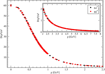
(a) Bare gluon propagator for both lattices.

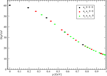
(b) $64^{4}$ propagator for different types of momenta.

Figure 2: Bare Landau gauge gluon propagator.

In Fig. 3 $\Gamma(p^{2})$ is plotted for different types of momenta. For the $64^{4}$ lattice, the data for $(n000)$ momenta does not follow the same curve as the other types of momenta. Furthermore, for the $80^{4}$ lattice, momenta of type $(n000)$ does not provide any useful information about the form factor. As a consequence, from now on we will disregard the momenta of type $(n000)$ in our analysis.

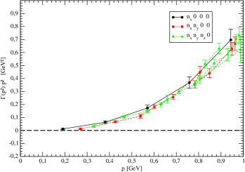
(a) $64^{4}$.

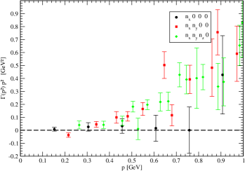
(b) $80^{4}$.

Figure 3: Infrared $\Gamma(p^{2})p^{2}$ for different types of momenta.

The form factor $\Gamma(p^{2})$ for both data sets and for momenta up to 2 GeV can be seen in Fig. 4. Although we see larger statistical errors for the larger volume, the results from the two lattice ensembles are essentially compatible within errors. In what concerns the behaviour in the low momenta region, we see a negative $\Gamma(p^{2})=-0.80(37)$ at $p=216$ MeV for the larger lattice. This value is compatible with zero only within 2.2 $\sigma$. Note that for higher momenta, we have $\Gamma(p=270\mbox{ MeV})=0.171(73)$ from the $64^{4}$ volume and $\Gamma(p=264\mbox{ MeV})=0.58(43)$ from the $80^{4}$ volume. In this sense, our data suggests that a zero crossing in $\Gamma(p^{2})$ should take place for $p\lesssim 250$ MeV. Earlier lattice simulations reported a zero crossing at essentially the same momentum value.

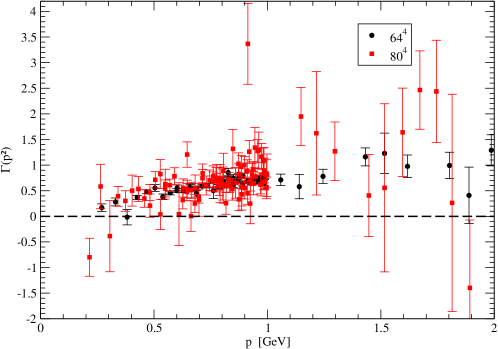
Figure 4: $\Gamma(p^{2})$ for the simulations considered in this work.

4 The ultraviolet region

The measurement of $\Gamma(p^{2})$ requires the computation of the ratio

$$\frac{G_{\mu\alpha\mu}(p,0,-p)p_{\alpha}}{\left[D(p^{2})\right]^{2}\,D(0)}.$$ (13)

This ratio induces large statistical fluctuations at high momenta. In fact, if we assume gaussian error propagation for the estimation of the statistical error on $\Gamma(p^{2})$, we obtain $\Delta\Gamma(p^{2})\sim p^{2}$. However, it is possible to measure the following combination

$$\Gamma_{UV}(p^{2})=\left[D(p^{2})\right]^{2}\,D(0)~{}\Gamma(p^{2})~{}p^{2}$$ (14)

with controllable statistical errors. Combining the predictions from one-loop renormalization group improved perturbation theory for $D(p^{2})$ and $\Gamma(p^{2})$, we get the following result for the behaviour of $\Gamma_{UV}(p^{2})$ at high momenta:

$$\Gamma_{UV}(p^{2})=\frac{Z}{p^{2}}\left[\ln\frac{p^{2}}{\mu^{2}}\right]^{\gamma^{\prime}}$$ (15)

where $\gamma^{\prime}=-35/44$, $Z$ is a constant and $\mu$ is a renormalization scale.

The results for $\Gamma_{UV}(p^{2})$ can be seen in Fig. 5 where we also show the prediction from tree-level perturbation theory $\Gamma_{UV}(p^{2})\sim\frac{1}{p^{2}}$ and the prediction of Eq. (15).

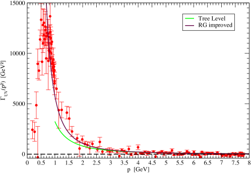
Figure 5: Comparison of $\Gamma_{UV}(p^{2})$ computed from the $64^{4}$ simulation with the predictions from perturbation theory.

5 Conclusions

We have computed the three gluon complete Green’s function on the lattice, for a particular kinematical configuration ($p_{2}=0$), using two different lattice volumes, $(6.5$ fm$)^{4}$ and $(8.2$ fm$)^{4}$ for the same lattice spacing ($a=0.102$ fm). In what concerns the low momenta region, we verified that the form factor $\Gamma(p^{2})$ exhibits a zero crossing for $p\sim 250$ MeV. Earlier results for 3d SU(2) [3, 4] and 4d SU(3) [5] lattice simulations are in good agreement with ours. We have also observed that, for sufficiently high momenta, the lattice data is compatible with the prediction of renormalisation group improved perturbation theory. More details about our work can be found in [14].

- [1] D. Binosi, D. Ibañez, and J. Papavassiliou, Phys. Rev. D87, 125026 (2013).
- [2] A. Aguilar, D. Binosi, D. Ibañez, and J. Papavassiliou, Phys. Rev. D89, 085008 (2014).
- [3] A. Cucchieri, A. Maas, T. Mendes, Phys. Rev. D74, 014503 (2006).
- [4] A. Cucchieri, A. Maas, T. Mendes, Phys. Rev. D77, 094510 (2008).
- [5] A. Athenodorou, D. Binosi, Ph. Boucaud, F. De Soto, J. Papavassiliou, J. Rodríguez-Quintero, and S. Zafeiropoulos, Phys. Lett. B761, 444 (2016) [arXiv:1607.01278 [hep-ph]].
- [6] André Sternbeck, Paul-Herrmann Balduf, these proceedings.
- [7] J. S. Ball, T.-W. Chiu, Phys. Rev. D22, 2550 (1980).
- [8] C. T. H. Davies, G. G. Batrouni, G. R. Katz, A. S. Kronfeld, G. P. Lepage, K. G. Wilson, P. Rossi, B. Svetitsky, Phys. Rev. D37, 1581 (1988).
- [9] R. G. Edwards, B. Joó (SciDAC Collaboration, LHPC Collaboration, UKQCD Collaboration), Nucl. Phys. Proc. Suppl. 140, 832 (2005) [arXiv:hep-lat/0409003].
- [10] M. Pippig, SIAM J. Sci. Comput. 35, C213 (2013).
- [11] B. Allés, D. S. Henty, H. Panagopoulos, C. Parrinello, C. Pittori, D. G. Richards, Nucl. Phys. B502, 325 (1997).
- [12] O. Oliveira, P. J. Silva, Phys. Rev. D86, 114513 (2012) [arXiv:1207.3029 [hep-lat]].
- [13] A. G. Duarte, O. Oliveira, P. J. Silva, Phys. Rev. D94, 014502 (2016) [arXiv:1605.00594 [hep-lat]].
- [14] A. G. Duarte, O. Oliveira, P. J. Silva, Phys. Rev. D94, 074502 (2016) [arXiv:1607.03831 [hep-lat]].
- [15] www.uc.pt/lca