Lasso, fractional norm and structured sparse estimation using a Hadamard product parametrization

Abstract

Using a multiplicative reparametrization, I show that a subclass of $L_{q}$ penalties with $q\leq 1$ can be expressed as sums of $L_{2}$ penalties. It follows that the lasso and other norm-penalized regression estimates may be obtained using a very simple and intuitive alternating ridge regression algorithm. As compared to a similarly intuitive EM algorithm for $L_{q}$ optimization, the proposed algorithm avoids some numerical instability issues and is also competitive in terms of speed. Furthermore, the proposed algorithm can be extended to accommodate sparse high-dimensional scenarios, generalized linear models, and can be used to create structured sparsity via penalties derived from covariance models for the parameters. Such model-based penalties may be useful for sparse estimation of spatially or temporally structured parameters.

Keywords: cyclic coordinate descent, generalized linear model, linear regression, optimization, ridge regression, sparsity, spatial autocorrelation.

1 Introduction

Consider estimation for the normal linear regression model $y\sim N_{n}(X\beta,\sigma^{2}I)$, where $X\in\mathbb{R}^{n\times p}$ is a matrix of predictor variables and $\beta\in\mathbb{R}^{p}$ is a vector of regression coefficients to be estimated. A least squares estimate is a minimizer of the residual sum of squares $||y-X\beta||^{2}.$ A popular alternative estimate is the lasso estimate (Tibshirani, 1996), which minimizes $||y-X\beta||^{2}+\lambda||\beta||_{1}$, a penalized residual sum of squares that balances fit to the data against the possibility that some or many of the elements of $\beta$ are small or zero. Indeed, minimizers of this penalized sum of squares may have elements that are exactly zero.

There exists a large variety of optimization algorithms for finding lasso estimates (see Schmidt et al. (2007) for a review). However, the details of many of these algorithms are somewhat opaque to data analysts who are not well-versed in the theory of optimization. One exception is the local quadratic approximation (LQA) algorithm of Fan and Li (2001), which proceeds by iteratively computing a series of ridge regressions. Fan and Li (2001) also suggested using LQA for non-convex $L_{q}$ penalization when $q<1$, and this technique was used by Kabán and Durrant (2008) and Kabán (2013) in their studies of non-convex $L_{q}$-penalized logistic regression. However, LQA can be numerically unstable for some combinations of models and penalties. To remedy this, Hunter and Li (2005) suggested optimizing a surrogate “perturbed” objective function. This perturbation must be user-specified, and its value can affect the parameter estimate. As an alternative to using local quadratic approximations, Zou and Li (2008) suggest $L_{q}$-penalized optimization using local linear approximations (LLA). While this approach avoids the instability of LQA, the algorithm is implemented by iteratively solving a series of $L_{1}$ penalization problems for which an optimization algorithm must be chosen as well.

This article develops a simple alternative technique for obtaining $L_{q}$-penalized regression estimates for many values of $q\leq 1$. The technique is based on a non-identifiable Hadamard product parametrization (HPP) of $\beta$ as $\beta=u\circ v$, where “$\circ$” denotes the Hadamard (element-wise) product of the vectors $u$ and $v$. As shown in the next section, if $\hat{u}$ and $\hat{v}$ are optimal $L_{2}$-penalized values of $u$ and $v$, then $\hat{\beta}=\hat{u}\circ\hat{v}$ is an optimal $L_{1}$-penalized value of $\beta$. An alternating ridge regression algorithm for obtaining $\hat{u}\circ\hat{v}$ is easy to understand and implement, and is competitive with LQA in terms of speed. Furthermore, a modified version of HPP can be adapted to provide fast convergence in sparse, high-dimensional scenarios. In Section 3 we consider extensions of this algorithm for non-convex $L_{q}$-penalized regression with $q\leq 1$. As in the $L_{1}$ case, $L_{q}$-penalized linear regression estimates may be found using alternating ridge regression, whereas estimates in generalized linear models can be obtained with a modified version of an iteratively reweighted least squares algorithm. In Section 4 we show how the HPP can facilitate structured sparsity in parameter estimates: The $L_{2}$ penalty on the vectors $u$ and $v$ can be interpreted as independent Gaussian prior distributions on the elements of $u$ and $v$. If instead we choose a penalty that mimics a dependent Gaussian prior, then we can achieve structured sparsity among the elements of $\hat{\beta}=\hat{u}\circ\hat{v}$. This technique is illustrated with an analysis of brain imaging data, for which a spatially structured HPP penalty is able to identify spatially contiguous regions of differential brain activity. A discussion follows in Section 5.

2 $L_{1}$ optimization using the HPP and ridge regression

2.1 The Hadamard product parametrization

The lasso or $L_{1}$-penalized regression estimate $\hat{\beta}$ of $\beta$ for the model $y\sim N_{p}(X\beta,\sigma^{2}I)$ is the minimizer of $||y-X\beta||^{2}+\lambda||\beta||_{1}$, or equivalently of the objective function

$$f(\beta)=\beta^{\top}Q\beta-2\beta^{\top}l+\lambda||\beta||_{1},$$ (1)

where $Q=X^{\top}X$ and $l=X^{\top}y$. Now reparametrize the model so that $\beta=u\circ v$, where “$\circ$” is the Hadamard (element-wise) product. We refer to this parametrization as the Hadamard product parametrization (HPP). Estimation of $u$ and $v$ using $L_{2}$ penalties corresponds to the following objective function:

$$g(u,v)=(u\circ v)^{\top}Q(u\circ v)-2(u\circ v)^{\top}l+\lambda(u^{\top}u+v^{\top}v)/2.$$ (2)

Consideration of this parametrization and objective function may seem odd, as the values of $u$ and $v$ beyond their element-wise product $\beta$ are not identifiable from the data. However, $g$ is differentiable and biconvex, and its local minimizers can be found using a very simple alternating ridge regression algorithm. Furthermore, there is a correspondence between minimizers of $g$ and minimizers of $f$, which we state more generally as follows:

Lemma 1.

Let $f(\beta)=h(\beta)+\lambda||\beta||_{1}$ and $g(u,v)=h(u\circ v)+\lambda(u^{\top}u+v^{\top}v)/2$. Then

1. $\inf_{\beta}f(\beta)=\inf_{u,v}g(u,v)$;

2. if $(\hat{u},\hat{v})$ is a local minimum of $g$, then $\hat{\beta}=\hat{u}\circ\hat{v}$ is a local minimum of $f$.

Proof.

To show item 1 we write $u=\beta/v$, where “$/$” denotes element-wise division, so that

$$\inf_{u,v}g(u,v) =\inf_{\beta,v}g(\beta/v,v)$$

$$=\inf_{\beta}\inf_{v}\left\{h(\beta)+\lambda\left(||\beta/v||^{2}+||v||^{2}\right)/2\right\}$$

$$=\inf_{\beta}\left\{h(\beta)+\lambda\inf_{v}\left(||\beta/v||^{2}+||v||^{2}\right)/2\right\}.$$

The inner infimum over $v$ is attained, and a minimizer $\tilde{v}$ can be can be found element-wise. The $j$th element $\tilde{v}_{j}$ of a minimizer $\tilde{v}$ is simply a minimizer of $\beta_{j}^{2}/v_{j}^{2}+v_{j}^{2}$. If $\beta_{j}$ is zero then $\tilde{v}_{j}=0$ is the unique global minimizer. Otherwise, this function is strictly convex in $v_{j}^{2}$ with a unique minimum at $\tilde{v}_{j}^{2}=|\beta_{j}|$. The inner minimum is therefore

$$||\beta/\tilde{v}||^{2}+||\tilde{v}||^{2} =\sum_{j=1}^{p}\left(\beta_{j}^{2}/\tilde{v}_{j}^{2}+\tilde{v}_{j}^{2}\right)$$

$$=\sum_{j=1}^{p}\left(\beta_{j}^{2}/|\beta_{j}|+|\beta_{j}|\right)=2||\beta||_{1},$$

and so

$$\inf_{u,v}g(u,v) =\inf_{\beta,v}g(\beta/v,v)$$

$$=\inf_{\beta}\left\{h(\beta)+\lambda\min_{v}\left(||\beta/v||^{2}+||v||^{2}\right)/2\right\}$$

$$=\inf_{\beta}\left\{h(\beta)+\lambda||\beta||_{1}\right\}=\inf_{\beta}f(\beta).$$

This proves item 1. In this proof, we saw that the constrained minimum of $u^{\top}u+v^{\top}v$ subject to $u\circ v=\beta$ is attained when $u_{j}^{2}=v_{j}^{2}=|\beta_{j}|$. Since $h$ only depends on $u\circ v$, a local minimizer $(\hat{u},\hat{v})$ of $g$ must also be a minimizer of $u^{\top}u+v^{\top}v$ subject to the constraint that $u\circ v=\hat{u}\circ\hat{v}=\hat{\beta}$, and so $\hat{u}_{j}^{2}=\hat{v}_{j}^{2}=|\hat{\beta}_{j}|$, giving a local minimum value of $g(\hat{u},\hat{v})=h(\hat{\beta})+\lambda||\hat{\beta}||_{1}=f(\hat{\beta})$. That this must be a local minimum of $f$ follows from the fact that the image of any ball in $\mathbb{R}^{p}\times\mathbb{R}^{p}$ around $(\hat{u},\hat{v})$ under the mapping $(u,v)\rightarrow u\circ v$ contains a ball in $\mathbb{R}^{p}$ around $\hat{u}\circ\hat{v}$. This proves item 2. ∎

We now return to the definitions of $f$ and $g$ in Equations (1) and (2), where $h(\beta)=\beta^{\top}Q\beta-2\beta^{\top}l$. Since all local minimizers of $f$ are global minimizers (Tibshirani, 2013), item 2 of the lemma shows that any local minimizer $(\hat{u},\hat{v})$ of $g$ provides a global optimizer $\hat{\beta}=\hat{u}\circ\hat{v}$ of the lasso objective function. In other words, lasso estimates can be obtained from local minimizers of $g$. Such minimizers can be found with a simple and intuitive alternating ridge regression algorithm. To see this, rewrite $(u\circ v)^{\top}Q(u\circ v)$ as $u^{\top}(Q\circ vv^{\top})u$, and $(u\circ v)^{\top}l$ as $u^{\top}(v\circ l)$, so that

$$g(u,v)=u^{\top}(Q\circ vv^{\top}+\tfrac{\lambda}{2})u+2u^{\top}(v\circ l)+\lambda v^{\top}v/2.$$

This is quadratic in $u$ for fixed $v$, with a unique minimizer of $\tilde{u}=(Q\circ vv^{\top}+\tfrac{\lambda}{2}I)^{-1}(l\circ v)$. Similarly, the unique minimizer of $g(u,v)$ in $v$ for fixed $u$ is $\tilde{v}=(Q\circ uu^{\top}+\tfrac{\lambda}{2}I)^{-1}(l\circ u)$. Iteratively optimizing $u$ and then $v$ given each other’s current value is a type of coordinate descent algorithm. Since each conditional minimizer is unique, the algorithm will converge to a stationary point $(\hat{u},\hat{v})$ of $g$ (Luenberger and Ye, 2008). At convergence, derivatives can be calculated to check if the point is a local minimizer (and therefore also a global minimizer). Alternatively, the optimality of $\hat{\beta}=\hat{u}\circ\hat{v}$ can be evaluated by checking if the Karush-Kuhn-Tucker (KKT) conditions are approximately met: Following Tibshirani (2013), the vector $\hat{\beta}$ is a global minimizer of $f$ if

$$2(l_{j}-[Q\hat{\beta}]_{j})/\lambda =\text{sign}(\hat{\beta}_{j})\ \text{if}\ \hat{\beta}_{j}\neq 0,$$ (3)

$$2(l_{j}-[Q\hat{\beta}]_{j})/\lambda \in[-1,1]\,\ \ \ \text{if}\ \hat{\beta}_{j}=0.$$ (4)

It is interesting to note that any stationary point $(\hat{u},\hat{v})$ of $g(u,v)$ will give a value $\hat{\beta}=\hat{u}\circ\hat{v}$ that satisfies (3). To see this, note that at a critical point we have $(Q\circ\hat{v}\hat{v}^{\top}+\tfrac{\lambda}{2}I)\hat{u}=l\circ\hat{v}$, which implies

$$\hat{u}_{j} =2\hat{v}_{j}(l_{j}-[Q(\hat{u}\circ\hat{v})]_{j})/\lambda.$$

Similarly, $\hat{v}_{j}=2\hat{u}_{j}(l_{j}-[Q(\hat{u}\circ\hat{v})]_{j})/\lambda$. If $\hat{\beta}_{j}=\hat{u}_{j}\hat{v}_{j}\neq 0$, then neither $\hat{u}_{j}$ nor $\hat{v}_{j}$ equal zero either, and so $\hat{u}_{j}/\hat{v}_{j}=2(l_{j}-[Q(\hat{u}\circ\hat{v})]_{j})/\lambda=\hat{v}_{j}/\hat{u}_{j}.$ This implies that $\hat{u}_{j}^{2}=\hat{v}_{j}^{2}$, or equivalently,

$$2(l_{j}-[Q\hat{\beta}]_{j})/\lambda=\frac{\hat{u}_{j}}{\hat{v}_{j}} =\frac{\text{sign}(\hat{u}_{j})}{\text{sign}(\hat{v}_{j})}$$

$$=\text{sign}(\hat{u}_{j}\hat{v}_{j})=\text{sign}(\hat{\beta}_{j}),$$

and so condition (3) is met. Not all stationary points will satisfy (4), though. For example, the point $(0,0)\in\mathbb{R}^{p}\times\mathbb{R}^{p}$ is a stationary point of $g$ but is not a local minimum and does not satisfy (4). However, in all of the numerical examples I have evaluated, the HPP algorithm has converged to objective function values that were as good or better than those of other algorithms.

2.2 Numerical evaluation

The HPP provides a simple, intuitive algorithm for obtaining lasso regression estimates. Given a starting value $v$ (such as one based on an OLS or ridge regression estimate), the algorithm is to iterate steps 1 and 2 below until a convergence criteria is met:

1. Set $u=(Q\circ vv^{\top}+\tfrac{\lambda}{2}I)^{-1}(l\circ v)$;

2. Set $v=(Q\circ uu^{\top}+\tfrac{\lambda}{2}I)^{-1}(l\circ u)$.

One justification of the HPP algorithm is that, for some researchers, optimization of $g$ via this HPP algorithm may be more intuitive and easier to code than alternative optimization schemes for $f$ that require an understanding of convex optimization. With this in mind, it is of interest to compare the convergence of the HPP algorithm to other intuitive and/or easy to implement algorithms. One such algorithm is the local quadratic approximation (LQA) algorithm of Fan and Li (2001), which also proceeds via iterative ridge regression. Specifically, one iteration of the LQA algorithm is as follows:

1. Compute $D=\text{diag}(|\beta_{1}|^{-1},\ldots,|\beta_{p}|^{-1});$

2. Set $\beta=(Q+\tfrac{\lambda}{2}D)^{-1}l$.

The idea behind this algorithm is that $\beta^{T}D\beta/2$ is a quadratic approximation to the $L_{1}$ penalty $||\beta||_{1}$ in a neighborhood around the current value of $\beta$. This algorithm can equivalently be interpreted as an EM algorithm for finding the posterior mode of $\beta$ under independent Laplace prior distributions on the elements of $\beta$ (Figueiredo, 2003). However, inspection of the algorithm reveals a potential problem: As entries of $\beta_{j}$ approach zero the corresponding diagonal entries of $D$ approach infinity, which could lead to numerical instability in the calculation of the update to $\beta$ in step 2 of the algorithm. In particular, the condition number of the matrix $Q+q\tfrac{\lambda}{2}D$ will generally approach infinity as entries of $\beta$ approach zero. Hunter and Li (2005) propose to remedy to this potential numerical instability of LQA by perturbing the update in step 2 so that $D$ remains bounded. In the context of $L_{1}$-penalized estimation, this modification amounts to replacing $|\beta_{j}|^{-1}$, the $j$th diagonal element of $D$, with $(|\beta_{j}|+\epsilon)^{-1}$, where $\epsilon$ is some small positive number, thereby ensuring that the condition number of $Q+\tfrac{\lambda}{2}D$ does not go to infinity. Note that in contrast, the matrices $Q\circ vv^{\top}+\tfrac{\lambda}{2}I$ and $Q\circ uu^{\top}+\tfrac{\lambda}{2}I$ in steps 1 and 2 of the HPP algorithm require no such modification, and remain well-conditioned as elements of $u$ or $v$ approach zero.

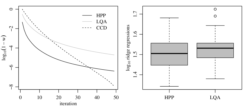
Figure 1: Simulation results for $L_{1}$-penalized regression. The left panel shows the progress of each algorithm per iteration, on average across the 100 datasets. The right panel shows the variability in the number of ridge regressions required until the convergence criterion is met.

Another natural candidate for comparison to the HPP algorithm is the “shooting” cyclic coordinate descent (CCD) algorithm described by Fu (1998). This algorithm optimizes the objective function iteratively for each element of $\beta$ using directional derivatives. While somewhat more complex than HPP and LQA in terms of understanding and implementation, CCD does not require matrix inversions and is perhaps the most popular algorithm for obtaining $L_{1}$-penalized regression coefficients.

The convergence properties of the HPP, CCD and $\epsilon$-perturbed LQA algorithms (with $\epsilon=10^{-12}$) were compared on 100 datasets that were simulated from the linear regression model $y\sim N_{n}(X\beta,I)$. A different value of $\beta$ was generated for each dataset, with entries simulated independently from a 50-50 mixture of a point-mass at zero and a mean-zero normal distribution with a standard deviation of 1/2. For each dataset, the entries of the design matrix $X$ were independently simulated from a standard normal distribution. Results are presented here for the case that $n=150$ and $p=100$. Other simulation scenarios may be explored using the replication code available at my website.

For each simulated dataset, a moment-based empirical Bayes estimate of $\lambda$ was obtained and all three algorithms were iterated 50 times, starting at the unpenalized least squares estimate. Let $f(\beta_{h}^{(i)})$, $f(\beta_{l}^{(i)})$ and $f(\beta_{c}^{(i)})$ denote the values of the objective function at the $i$th iterate of the HPP, LQA and CCD algorithms, respectively. Letting $f_{\max}=\max\{f(\beta_{h}^{(1)}),f(\beta_{l}^{(1)}),f(\beta_{c}^{(1)})\}$ and $f_{\min}=\min\{f(\beta_{h}^{(50)}),f(\beta_{l}^{(50)}),f(\beta_{s}^{(50)})\}$, the value of $w^{i}_{h}=(f_{\max}-f(\beta_{h}^{(i)}))/(f_{\max}-f_{\min})\in[0,1]$ measures the progress of the HPP algorithm at iterate $i$, and $w_{l}^{i}$ and $w_{c}^{i}$ can be defined similarly for the LQA and CCD algorithms. The upper-left panel of Figure 1 plots the values of $w_{h}^{i}$, $w_{l}^{i}$ and $w_{c}^{i}$ for each iteration $i$, on average across the 100 simulated datasets. The HPP algorithm makes substantially faster progress than either of the other two algorithms initially. However, HPP requires two ridge regressions per iteration, whereas LQA requires only one. To compare the computational costs of these algorithms, we need to evaluate the number of iterations each requires to find a solution. To this end, each of the three algorithms was iterated until

$$\max_{j}\left\{(\beta^{(i)}_{j}-\beta^{(i+1)}_{j})^{2}\sum_{k=1}^{n}x_{k,j}^{2}\right\}\leq\delta,$$ (5)

where $\delta$ was taken to be $\delta=10^{-6}$. The left side of this inequality is the convergence statistic used by the R-package glmnet (Friedman et al., 2010).

Objective functions and parameter estimates at convergence were compared across all three algorithms, and there was no evidence of any substantial differences: Relative differences in objective function values were below 0.001% $(10^{-5})$ for all 100 datasets, and relative squared differences among parameter estimates $\hat{\beta}$ and fitted values $X\hat{\beta}$ were also all less than 0.001%. The relative mean-squared estimation error $||\hat{\beta}-\beta||^{2}/||\beta||^{2}$ and the mean-squared prediction error $||X(\hat{\beta}-\beta)||^{2}/||X\beta||^{2}$ were 0.083 and 0.084, respectively, for all three algorithms.

The median numbers of iterations until convergence criterion (5) was met were 16, 34 and 29 for HPP, LQA and CCD respectively. The variability in the number of iterations until convergence for HPP and LQA is displayed in the second panel of Figure 1, where for comparison the results are given in terms of the number of ridge regressions required until convergence. Roughly speaking, HPP takes twice as much time per iteration but requires slightly less than half as many iterations to converge, resulting in a small reduction in average computational costs relative to LQA.

The computational costs of CCD are hard to compare to those of HPP and LQA as CCD involves different types of calculations at each iteration: CCD updates each of the $p$ coefficients cyclically, whereas HPP and LQA update multiple parameters at once but require matrix inversions at each iteration. An informal comparison on my desktop computer gave the total run-time to convergence for all 100 datasets being 0.96, 1.10 and 3.40 seconds for the HPP, LQA and CCD algorithms respectively, using convergence criteria (5) with $\delta=10^{-6}$. All algorithms were coded in the R programming environment using no C or FORTRAN code. It is likely that the runtime of CCD would improve relative to the other methods if such code were used, as each iteration of CCD involves a for-loop over the elements of $\beta$ which is particularly slow in R.

2.3 HPP for sparse high-dimensional regression

While simple to explain and implement, the HPP algorithm requires two matrix inversions per iteration and so becomes increasing computationally costly as $p$ increases. Such costs can be reduced by updating $u$ and $v$ via Cholesky decompositions instead of matrix inversions (see the replication code for details), but these calculations still require $O(p^{3})$ operations per decomposition.

However, the structure of the HPP algorithm permits a modification that can substantially reduce computational costs in sparse high-dimensional settings. Recall that the HPP update for the vector $u$ is $u=(Q\circ vv^{\top}+\tfrac{\lambda}{2}I)^{-1}(l\circ v)$, with an analogous update for $v$. If $v$ is sparse then so is $l\circ v$, and the rows and columns of the matrix $(Q\circ vv^{\top}+\tfrac{\lambda}{2}I)$ can be reordered to yield a block diagonal matrix with one block being $\lambda/2$ times an identity matrix. From this we can see that the elements of the updated $u$-vector corresponding the zero elements of $v$ will also be zero, while the remaining elements of $u$ will be given by $\tilde{u}=(\tilde{Q}\circ\tilde{v}\tilde{v}^{\top}+\tfrac{\lambda}{2}I)^{-1}(\tilde{l}\circ\tilde{v}),$ where $\tilde{Q}$, $\tilde{l}$, and $\tilde{v}$ are the submatrix and subvectors of $Q$, $l$, and $v$ corresponding to the non-zero elements of $v$. If the number of non-zero elements of $v$ is small, then the HPP update for $\tilde{u}$ (and thus $u$) can be computed quickly. Such a simplification is also possible for LQA in a limiting sense: If $D=\text{diag}(|\beta_{1}|^{-1},\ldots,|\beta_{p}|^{-1})$ then the LQA update matrix $(Q+\tfrac{\lambda}{2}D)^{-1}$ gets closer to being block diagonal as the elements of $\beta$ approach zero.

Unfortunately, these algorithms cannot take advantage of sparsity because neither algorithm produces coefficient updates that are exactly zero. A simple way to overcome this limitation is to set parameter values to zero if they are less in absolute value than some prespecified threshold. While this ad-hoc solution can induce exact sparsity, the caveat is that in doing so the algorithm may get trapped: Once an entry of $u$ or $v$ is set to zero, it remains zero for all iterations of HPP that follow. An easy fix to this potential problem is to induce sparsity not by ad-hoc thresholding, but by performing a CCD step, which can update a parameter from sparse to non-sparse and vice-versa. One version of such a mixed algorithm is to alternate HPP and CCD steps, resulting in what may be called an “HPCD” algorithm (Hadamard product, cyclic descent). Given a current value of $\beta$, two consecutive iterations of an HPCD algorithm proceeds as follows:

1. Update each element of $\beta$ iteratively with CCD.

2. Let $\tilde{\beta}$ be the nonzero values of $\beta$ and $\tilde{v}$ be the square root of the absolute values of $\tilde{\beta}$.

   1. Set $\tilde{u}=(\tilde{Q}\circ\tilde{v}\tilde{v}^{\top}+\tfrac{\lambda}{2}I)^{-1}(\tilde{l}\circ\tilde{v})$;

   2. Set $\tilde{v}=(\tilde{Q}\circ\tilde{u}\tilde{u}^{\top}+\tfrac{\lambda}{2}I)^{-1}(\tilde{l}\circ\tilde{u})$;

   3. Set $\tilde{\beta}=\tilde{u}\circ\tilde{v}$.

Similarly, an “LQCD” algorithm (local quadratic approximation, cyclic descent) may be constructed by alternately performing a CCD update and then an LQA update on the non-zero coefficients.

The HPCD, LQCD and CCD algorithms were compared in a simulation study of 100 datasets, simulated as before except now $p=1000$. Each algorithm was iterated 300 times on all 100 datasets, and the per-iteration convergence progress was averaged across datasets in the same manner as in the previous simulation study. The results, displayed graphically in the left panel of Figure 2,

Figure 2: Simulation results for $L_{1}$-penalized regression with $p>n$. The left panel shows the progress of each algorithm per iteration, on average across the 100 datasets. The right panel shows the time in seconds to convergence of each algorithm, across datasets.

indicate that on a per-iteration basis HPCD faster than LQCD and substantially faster than CCD.

The algorithms were also implemented on each dataset until convergence criteria (5) was met, with $\delta=10^{-6}$ as before. The three algorithms attained nearly the same objective function values as each other for each dataset, with relative differences being less than 0.001% ($10^{-5}$) across all datasets. Relative squared differences among parameter estimates $\hat{\beta}$ and fitted values $X\hat{\beta}$ were less than $1\%$ for all simulated datasets. Relative mean-squared estimation and prediction errors were 1.11 and 1.09 respectively, for all algorithms. The median number of iterations until convergence were 328, 649 and 1638 for the HPCD, LQCD and CCD algorithms respectively. The computational costs per iteration of these algorithms are difficult to compare since the sizes of the matrices inverted by HPCD and LQCD vary with the sparsity level of the parameter estimate. However, the amount of computer time until convergence was recorded for each algorithm and dataset, and is displayed graphically in the right panel of Figure 2. The HPCD algorithm was about 60% faster than LQCD on average, and more than five times faster than CCD (when implemented in R).

2.4 Correlated predictors

Since each iteration of CCD updates one element of $\beta$ at a time, its convergence properties may suffer if the Hessian of the objective function is not well conditioned. This can occur if the columns of $X$ are correlated (Friedman et al., 2010). Conversely, HPP and LQA both update entire vectors of parameters at once, and so their convergence properties may be robust to correlation among the predictors. We investigate this briefly with two simulation studies that are identical to the previous two, except now each $X$ is a column-standardized version of the random matrix $UV^{\top}+E$ where $U\in\mathbb{R}^{n\times r}$, $V\in\mathbb{R}^{p\times r}$ and $E\in\mathbb{R}^{n\times p}$ are matrices with i.i.d. standard normal entries, with $r=p/10$. To see how this produces correlated predictors, note that for fixed $V$ the rows of $UV^{\top}+E$ have covariance $VV^{\top}+I$.

As before, the different algorithms were applied to each simulated dataset for a fixed number of iterations, and their per-iteration progress towards the optimal objective function was averaged across datasets. Results for the $p=100$ simulation study are shown in the left panel of Figure 3. Comparing this to the left panel of Figure 1, the relative convergence rate of CCD is substantially reduced as compared to the case of uncorrelated predictors. The median numbers of iterations to convergence were 35, 74 and 192 for HPP, LQA and CCD respectively, representing a roughly two-fold increase for HPP and LQA but more than a six-fold increase for CCD.

The second panel of the figure compares HPCD, LQCD and CCD in the case that $p=1000$. The performance of CCD is much worse than HPCD and LQCD on a per-iteration basis, even more so than in the previous study with $p=1000$ (see Figure 2). The median numbers of iterations to convergence for HPCD, LQCD and CCD for this simulation study were 240, 458 and 2427. This represents a decrease in the number of iterations until convergence for HPCD and LQCD as compared to the uncorrelated case, but the number of iterations needed by CCD is now roughly 10 times that of HPCD. Average time to convergence was 3.2, 4.9 and 32.0 seconds for HPCD, LQCD and CCD respectively, and so for this simulation scenario HPCD is about 50% faster than LQCD, and 10 times faster than CCD as implemented in R.

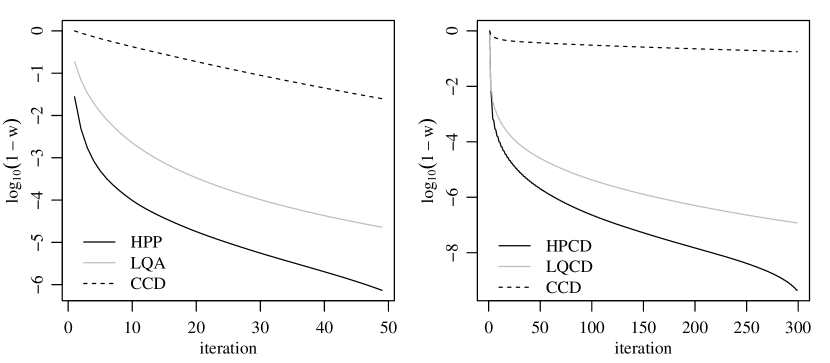
Figure 3: Average convergence progress for $L_{1}$-penalized regression algorithms with correlated predictors. The $p=100$ scenario is on the left, the $p=1000$ scenario is on the right.

3 HPP for non-convex penalties

3.1 HPP for $L_{q}$-penalized linear regression

A natural generalization of the HPP is to write $\beta=u_{1}\circ\cdots\circ u_{K}$ and optimize

$$g(u_{1},\ldots,u_{K})=(u_{1}\circ\cdots\circ u_{K})^{\top}Q(u_{1}\circ\cdots\circ u_{K})-2(u_{1}\circ\cdots\circ u_{K})^{\top}l+\tfrac{\lambda}{K}\left(u_{1}^{\top}u_{1}+\cdots u_{K}^{\top}u_{K}\right).$$ (6)

For $K=1$ the optimal $u$-value is the $L_{2}$-penalized ridge regression estimate, and for $K=2$ the optimal value of $(u_{1},u_{2})$ gives the $L_{1}$-penalized lasso regression estimate, as discussed in the previous section. Values of $K$ greater than 2 correspond to non-convex $L_{q}$ penalties with $q=2/K$. For example, the $L_{1/2}$-penalized estimate is obtained by optimizing (6) with $K=4$. Non-convex penalties such as these have been studied by Fan and Li (2001), Hunter and Li (2005), Kabán and Durrant (2008), Zou and Li (2008), and Kabán (2013) among others. Such non-convex penalties induce sparsity without the severe penalization of large parameter values that is imposed by convex penalties, such as the $L_{1}$ and $L_{2}$ norms. Defining $||\beta||_{q}^{q}=\sum_{j}|\beta_{j}|^{q}$, the correspondence between the $L_{q}$ penalties and the HPP is given by the following lemma:

Lemma 2.

Let $f(\beta)=h(\beta)+\lambda||\beta||_{q}^{q}$ where $q=2/K$, and let $g(u_{1},\ldots,u_{K})=h(u_{1}\circ\cdots\circ u_{K})+\lambda(u_{1}^{\top}u_{1}+\cdots u_{K}^{\top}u_{K})/K$. Then

1. $\inf_{\beta}f(\beta)=\inf_{u_{1},\ldots,u_{K}}g(u_{1},\ldots,u_{K})$;

2. if $(\hat{u}_{1},\ldots,\hat{u}_{K})$ is a local minimum of $g$, then $\hat{\beta}=\hat{u}_{1}\circ\cdots\circ\hat{u}_{K}$ is a local minimum of $f$.

Proof.

Using Lagrange multipliers, it is straightforward to show that the minimum value of $\sum_{k}u_{k}^{\top}u_{k}$ subject to the constraint that $\prod_{k}u_{k,j}=\beta_{j}$ is attained when $|u_{k,j}|$ is constant across $k$. This implies that at a minimizing value, $u_{k,j}^{2}=|\beta_{j}|^{2/K}$ and that $\sum_{k}u_{k}^{\top}u_{k}=||\beta||_{q}^{q}$, where $q=2/K$. The lemma then follows using exactly the same logic as used to prove Lemma 1. ∎

The lemma suggests a simple alternating ridge regression algorithm for obtaining $L_{q}$-penalized linear regression estimates in cases where $q=2/K$ for some integer $K$. Given a starting value $(u_{2},\ldots,u_{K})$, repeat steps 1 and 2 below for each $k=1,\ldots,K$, iteratively until convergence:

1. Set $v=(u_{1}\circ\cdots\circ u_{K})/u_{k}$;

2. Set $u_{k}=(Q\circ vv^{T}+\tfrac{\lambda}{K}I)^{-1}(l\circ v)$.

Note that $v$ in item 1 is simply the Hadamard product of the vectors $\{u_{1},\ldots,u_{K}\}$ except for $u_{k}$. Another intuitive algorithm that is even easier to code is the LQA algorithm for $L_{q}$-penalized linear regression, which proceeds by iterating the following steps:

1. Compute $D=\text{diag}(|\beta_{1}|^{q-2},\ldots,|\beta_{p}|^{q-2});$

2. Set $\beta=(Q+q\tfrac{\lambda}{2}D)^{-1}l$.

As discussed in the previous section, the condition number of $Q+q\tfrac{\lambda}{2}D$ in step 2 of the algorithm will generally converge to infinity as elements of $\beta$ approach zero, leading to the potential for numerical instability. The $\epsilon$-perturbed version of this algorithm proposed by Hunter and Li (2005) is to replace $|\beta_{j}|^{q-2}$, the $j$th diagonal element of $D$, with $|\beta_{j}|^{q-2}\tfrac{|\beta_{j}|}{|\beta_{j}|+\epsilon}$, where $\epsilon$ is some small positive number. While this term no longer remains bounded as $|\beta_{j}|\rightarrow 0$ if $q<1$, it does result in a minorization-maximization algorithm for optimizing a perturbed version of the objective function (see Hunter and Li (2005) for details). An alternative to LQA is the local linear approximation method (LLA) of Zou and Li (2008). For $L_{q}$-penalized regression, the LLA algorithm consists of iteratively solving an $L_{1}$-penalized regression problem as follows:

1. Compute $D=\text{diag}(|\beta_{1}|^{q-1},\ldots,|\beta_{p}|^{q-1});$

2. Set $\beta=\arg\min_{\beta}\beta^{\top}Q\beta-2\beta^{\top}l+2q\lambda\sum_{j=1}^{p}d_{j}|\beta_{j}|.$

As described by Zou and Li (2008), this approach avoids the potential numerical instability of the LQA algorithm, but requires an $L_{1}$-optimization at each iteration.

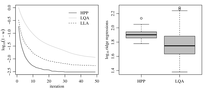
Figure 4: Simulation results for $L_{1/2}$-penalized regression. The left panel shows the progress of each algorithm per iteration, on average across the 100 datasets. The right panel shows the variability in the number of ridge regressions required until the convergence criterion is met.

The convergence properties of HPP, LLA and $\epsilon$-perturbed LQA were compared on the same simulated datasets as described in Section 2.2, but now using a nonconvex $L_{1/2}$ penalty corresponding to $K=4$. A summary of the results are displayed in Figure 4. As can be seen in the left panel, HPP converges at a faster rate per iteration than LQA, on average across datasets. Iterating until convergence, relative differences in objective function values were all below .4% $(0.004)$, and relative squared differences among parameter estimates $\hat{\beta}$ and fitted values $X\hat{\beta}$ were less than 1% for all but one of the simulated datasets. Relative mean-squared estimation error and prediction error were 0.081 and 0.082, respectively, for all three algorithms.

The median numbers of iterations until convergence were 20, 56 and 22 for the HPP, LQA and LLA algorithms respectively. Using the convergence criteria (5) with $\delta=10^{-6}$, the LQA algorithm required slightly more than three times (3.26) as many iterations as HPP to converge, on average across datasets. However, HPP requires $K=4$ ridge regressions per iteration as compared to one for LQA. Taking this into account, the two algorithms are comparable in terms of computational burden, as shown in the right panel of Figure 4, with the LQA algorithm being slightly more efficient on average. While the computational costs of HPP and LQA are easy to compare to each other, the cost of LLA is not easily comparable, as this algorithm involves different operations than the other two and depends on the particular $L_{1}$-optimization method being used. I compared the computational costs of LLA to HPP and LQA in terms of their runtimes on my desktop computer, using the R-package penalized (Goeman et al., 2016) to implement the $L_{1}$-optimization required by LLA. The total elapsed time to convergence, summed over all 100 simulated datasets, was 3.3 and 2.2 seconds for HPP and LQA respectively, whereas for LLA it was 15.0 seconds. The relative lack of speed of the LLA algorithm is due to the fact that, for these values of $n$ and $p$, performing an $L_{1}$-optimization at each iteration is much more costly than performing the single Cholesky factorization needed by HPP and LQA at each iteration. For larger values of $p$ where Cholesky factorizations are more costly, the LLA algorithm will be more competitive with HPP and LQA.

3.2 HPP for $L_{q}$-penalized generalized linear models

The arbitrariness of the function $h(\beta)$ in Lemmas 1 and 2 means that the HPP could be used for penalized estimation in scenarios beyond linear regression. Consider a likelihood $L(\beta,\psi)=\prod_{i}p(y_{i}|\eta_{i},\psi)$ where $\eta_{i}=\beta^{\top}x_{i}$ and $p(y_{i}|\eta_{i},\psi)=c(y_{i})e^{\{(y_{i}\eta_{i}-A(\eta_{i}))/\psi\}}$, with $x_{i}$ being an observed $p$-variate vector of predictors for each observation $i$. The $L_{q}$-penalized likelihood estimate of $\beta$ is the maximizer of the penalized likelihood given by $\exp(-\lambda||\beta||_{q}^{q}/(2\psi))\times\prod_{i}p(y_{i}|\eta_{i},\psi)$, or equivalently is the minimizer of two times the scaled negative log penalized likelihood

$$f(\beta)=2\sum_{i}A(\beta^{\top}x_{i})-2\beta^{\top}\sum_{i}y_{i}x_{i}+\lambda||\beta||_{q}^{q}.$$

For example, the special cases of linear regression, Poisson regression and logistic regression correspond to $A(\eta)$ being equal to $\eta^{2}/2$, $e^{\eta}$ and $\ln(1+e^{\eta})$ respectively.

By Lemma 2, if $q=2/K$ then the minimum of $f(\beta)$ is equal to the minimum of $g(u_{1},\ldots,u_{K})$, where

$$g(u_{1},\ldots,u_{K})=2\sum_{i}A([u_{1}\circ\cdots\circ u_{K}]^{\top}x_{i})-2(u_{1}\circ\cdots\circ u_{K})^{\top}X^{\top}y+\frac{\lambda}{K}\left(u_{1}^{\top}u_{1}+\cdots u_{K}^{\top}u_{K}\right).$$

Local minima of $g$ can be found using a variety of algorithms that iteratively update $u_{1},\ldots,u_{K}$. For example, suppose we can optimize the following $L_{2}$-penalized likelihood function in $\beta$:

$$f(\beta:X,\lambda)=2\sum_{i}A(\beta^{\top}x_{i})-2\beta^{\top}X^{\top}y+\lambda||\beta||^{2}.$$

Now let $v=(u_{1}\circ\cdots\circ u_{K})/u_{k}$. The part of $g$ that depends on $u_{k}$ can be written as

$$g_{k}(u_{k}:X,v) =2\sum_{i}A([u_{k}\circ v]^{\top}x_{i})-2(u_{k}\circ v)^{\top}\sum_{i}y_{i}x_{i}+\tfrac{\lambda}{K}u_{k}^{\top}u_{k}$$

$$=2\sum_{i}A(u_{k}^{\top}[v\circ x_{i}])-2u_{k}^{\top}\sum_{i}y_{i}(v\circ x_{i})+\tfrac{\lambda}{K}u_{k}^{\top}u_{k}$$

$$=f(u_{k}:\tilde{X}_{k},\lambda/K),$$

where $\tilde{X}_{k}=XD(v)$, so that the $i$th row of $\tilde{X}_{k}$ is $\tilde{x}_{i}=v\circ x_{i}$. If we can optimize $f(\beta:X,\lambda)$ in $\beta$, then we can optimize $g$ by iteratively optimizing $f(u_{k}:\tilde{X}_{k},\lambda/K)$ in $u_{k}$ for each $k=1,\ldots,K$. Therefore, any algorithm that provides $L_{2}$-penalized generalized linear model estimates can also be used to provide $L_{q}$-penalized estimates via the HPP, if $q=2/K$. For example, $f(u_{k}:\tilde{X}_{k},\lambda/K)$ can generally be optimized with the Newton-Raphson algorithm. The first and second derivatives of $f(u_{k}:\tilde{X}_{k},\lambda/K)$ are

$$d_{k}=\frac{\partial f}{\partial u_{k}}= 2\left(v\circ\sum x_{i}(\dot{A}(\eta_{i})-y_{i})+\tfrac{\lambda}{K}u_{k}\right)$$

$$H_{k}=\frac{\partial^{2}f}{\partial u_{k}\partial u_{k}^{T}} =2\left(vv^{T}\circ\sum\ddot{A}(\eta_{i})x_{i}x_{i}^{T}+\tfrac{\lambda}{K}I\right),$$

where $\eta_{i}=(u_{1}\circ\cdots\circ u_{K})^{T}x_{i}$ and $\dot{A}$ and $\ddot{A}$ are the first and second derivatives of $A(\eta)$, respectively. Critical points of $g$ can then be found by repeating the following steps iteratively for $i=1,\ldots,K$ until convergence:

1. Compute $v=(u_{1}\circ\cdots\circ u_{K})/u_{k}$;

2. Optimize $f(u_{k}:\tilde{X}_{k},\lambda/K)$ in $u_{k}$ by iterating the following until convergence:

   1. Compute $\eta_{i}=(u_{k}\circ v)^{\top}x_{i}$ for each $i=1,\ldots,n$, then $d_{k}$ and $H_{k}$;

   2. Set $u_{k}$ to $u_{k}-H_{k}^{-1}d_{k}$.

The LQA strategy for $L_{q}$-penalized estimation in generalized linear models is similar, except that at each iteration we optimize

$$2\sum_{i}A(\beta^{\top}x_{i})-2\beta^{\top}\sum y_{i}x_{i}+q\lambda\beta^{\top}D\beta,$$

where $D=\text{diag}(|\tilde{\beta}_{1}|^{q-2},\ldots,|\tilde{\beta}_{p}|^{q-2})$, with $\tilde{\beta}$ being the value of $\beta$ at the current iteration of the algorithm. The $\epsilon$-perturbed version of this LQA algorithm is, as in the previous subsection, obtained by replacing $|\beta_{j}|^{q-2}$, the $j$th diagonal element of $D$, with $|\beta_{j}|^{q-2}\tfrac{|\beta_{j}|}{|\beta_{j}|+\epsilon}$, where $\epsilon$ is some small positive number. This perturbed LQA algorithm with $\epsilon=10^{-12}$ was compared to the HPP and LLA algorithms in terms of obtaining $L_{1/2}$-penalized estimates of logistic regression coefficients. For each of the 100 values of $\beta$ and $X$ used in the previous simulation study, a vector of $n=150$ binary observations were independently simulated from the logistic regression model $y_{i}\sim\text{binary}(e^{\beta_{i}^{\top}x_{i}}/(1+e^{\beta_{i}^{\top}x_{i}}))$, for $i=1,\ldots,n$. As shown in the left panel of Figure 5, each iteration of HPP provides a larger improvement to the objective function than an iteration of either LLA or LQA, on average across datasets. Each of the three algorithms were also iterated until convergence criteria (5) was met. Unlike for the previous three simulation studies, the objective functions at convergence were sometimes non-trivially different: Objective functions differed by as much as 4.3%, and differed by 1% or more for 18 of the 100 datasets. The HPP algorithm attained a lower (better) objective function than the LQA algorithm for 88 of the 100 datasets, and a lower objective function than LLA for 60 datasets. However, even though these algorithms produced solutions with non-trivial objective function differences, their estimation accuracies were nearly identical: Relative MSE $||\hat{\beta}-\beta||^{2}/||\beta||^{2}$ and the mean function estimation error $||X(\hat{\beta}-\beta)||^{2}/||X\beta||^{2}$ were both about 0.78 on average across datasets for all three methods.

While the number of iterations to convergence for the LQA algorithm was nearly five times (4.65) that of the HPP algorithm on average, HPP requires $K=4$ Newton-Raphson optimizations per iteration whereas LQA only requires one. As shown in the right panel of the figure, this results in the HPP algorithm being slightly less computationally costly than the LQA algorithm, on average. In term of comparison to LLA, while for linear regression the computational costs per iteration of HPP and LQA were much lower than that of LLA, for logistic regression the converse is true: In terms of elapsed times to convergence, HPP and LQA took a total of 27.5 and 30.2 seconds respectively to obtain estimates for all 100 datasets, whereas LLA took only 14.7 seconds - about twice as fast for this particular simulation scenario. This reversal is because all three logistic regression algorithms involve iterative optimization schemes within each iteration (IRLS for HPP and LQA, gradient descent for LLA), whereas for linear regression this was the case only for LLA.

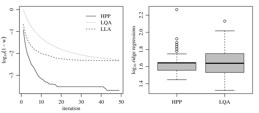
Figure 5: Simulation results for $L_{1/2}$-penalized logistic regression. The left panel shows the progress of each algorithm per iteration, on average across the 100 datasets. The right panel shows the variability in the number of ridge regressions required until the convergence criterion is met.

4 Structured penalization with the HPP

It is well-known that the lasso objective function $f(\beta)=\beta^{T}Q\beta-2\beta^{T}l+\lambda||\beta||_{1}$ is equal to the scaled log posterior density of $\beta$ under a Laplace prior distribution on the elements of $\beta$ (Tibshirani, 1996; Figueiredo, 2003; Park and Casella, 2008). Specifically, for the linear regression model $y\sim N(X\beta,\sigma^{2}I)$ and prior distribution $\beta_{1},\ldots,\beta_{p}\sim$ i.i.d. Laplace$(\lambda/[2\sigma^{2}])$, the posterior density of $\beta$ is given by

$$p(\beta|y,X,\sigma^{2}) \propto\exp(-||y-X\beta||^{2}/[2\sigma^{2}])\exp(-\lambda||\beta||_{1}/[2\sigma^{2}])$$

$$\propto\exp(-\tfrac{1}{2\sigma^{2}}[\beta^{\top}Q\beta-2\beta^{\top}l+\lambda||\beta||_{1}])=\exp(-\tfrac{1}{2\sigma^{2}}f(\beta)),$$

where $Q=X^{\top}X$ and $l=X^{\top}y$ as before. The lasso estimate $\hat{\beta}$ is therefore equal to the posterior mode estimate. Alternatively, reparametrizing the regression model so that $\beta=u\circ v$, and using independent $N(0,2\sigma^{2}/\lambda)$ prior distributions for the elements of $u$ and $v$ gives

$$p(u,v|y,X,\sigma^{2}) \propto\exp(-||y-X(u\circ v)||^{2}/[2\sigma^{2}])\exp(-\tfrac{1}{2\sigma^{2}}[\lambda u^{\top}u/2+\lambda v^{\top}v/2])$$

$$\propto\exp(-\tfrac{1}{2\sigma^{2}}g(u,v)),$$

where $g(u,v)=(u\circ v)^{T}Q(u\circ v)-2(u\circ v)^{T}l+\lambda(u^{\top}u+v\top v)/2$. The minimizers $\hat{u}$ and $\hat{v}$ of $g(u,v)$ may therefore be viewed as posterior mode estimates under independent Gaussian priors on $u$ and $v$, with the lasso estimate given by $\hat{\beta}=\hat{u}\circ\hat{v}$.

The $L_{1}$ and $L_{2}$ penalties (or Laplace and Gaussian priors) on $\beta$ and $(u,v)$ respectively induce sparsity in the parameter estimates, but in an unstructured way. From a Bayesian perspective, the a priori independence of the parameters means that the parameters convey no information about each other. In particular, the shrinkage of any one parameter is unrelated to that of any other. However, in many estimation problems there are relationships among the elements of $\beta$, and it may be desirable to shrink related parameters by similar amounts or towards a common value. For example, a subset of elements of $\beta$ may correspond to the effects of different levels of a single categorical predictor. For models with such variables, the group lasso penalty of Yuan and Lin (2006) may shrink the entire subset to zero, in which case it would be inferred that there is no effect of the categorical predictor. In other situations, the elements of $\beta$ may represent variables that have spatial or temporal locations. To estimate such parameters, Tibshirani et al. (2005) introduced the fused lasso, which in addition to penalizing the magnitudes of the elements of $\beta$, also penalizes the differences between elements that are spatially or temporally close to one another.

These and other structured penalizations employ a variety of optimization techniques to obtain parameter estimates. As an alternative to these approaches, the HPP can be used to generate a class of structured sparse estimates that can be obtained with a simple and intuitive alternating ridge regression algorithm. Consider the objective function

$$g(u,v)=(u\circ v)^{T}Q(u\circ v)-2(u\circ v)^{T}l+u^{\top}\Sigma_{u}^{-1}u+v^{\top}\Sigma_{v}^{-1}v,$$ (7)

where $\Sigma_{u}$ and $\Sigma_{v}$ are positive definite (covariance) matrices. This objective function is equal to the scaled log-posterior density of $(u,v)$ under the model $y\sim N(X\beta,\sigma^{2}I)$ and independent prior distributions $u/\sigma\sim N(0,\Sigma)$, $v/\sigma\sim N(0,\Sigma)$. We refer to this combination of parametrization and penalty as a structured HPP, or SHPP. Note that the unstructured HPP corresponding to the $L_{1}$ penalty on $\beta=u\circ v$ is obtained by setting $\Sigma=\tfrac{2}{\lambda}I$.

Local minima of $g(u,v)$ may be obtained with the following algorithm in which $u$ and $v$ are iteratively optimized until convergence:

1. Set $u=(Q\circ vv^{\top}+\Sigma_{u}^{-1})^{-1}(l\circ v)$;

2. Set $v=(Q\circ uu^{\top}+\Sigma_{v}^{-1})^{-1}(l\circ u)$.

In addition to the simplicity of the estimation approach, the SHPP also benefits from having a penalty that is easily interpretable as a covariance model for the relationships among the entries of $u$ and $v$, and therefore among the entries of $\beta=u\circ v$. From a Bayesian perspective, if $u/\sigma\sim N(0,\Sigma_{u})$ and $v/\sigma\sim N(0,\Sigma_{v})$, then ${\text{Cov}}[\beta/\sigma^{2}]=\Sigma_{u}\circ\Sigma_{v}$ (although $\beta$ is not a priori Gaussian). Furthermore, since any positive definite matrix can be written as the Hadamard product of two other positive definite matrices (Majindar, 1963; Styan, 1973), $\Sigma_{u}$ and $\Sigma_{v}$ can always be chosen to yield a particular value of ${\text{Cov}}[\beta/\sigma^{2}]$.

To illustrate the SHPP methodology, we analyze spatial data from a diffusion tensor imaging (DTI) study that compared the brain activity of 6 dyslexic children to that of 6 non-dyslexic controls, as described in Deutsch et al. (2005). Following Efron (2010), we analyze $z$-scores obtained from two-sample tests performed at each of $p=15,443$ spatially arranged voxels. Each voxel has a location in a $73\times 55\times 20$ three-dimensional grid. A plot of these $z$-scores at three adjacent vertical locations is given in Figure 6.

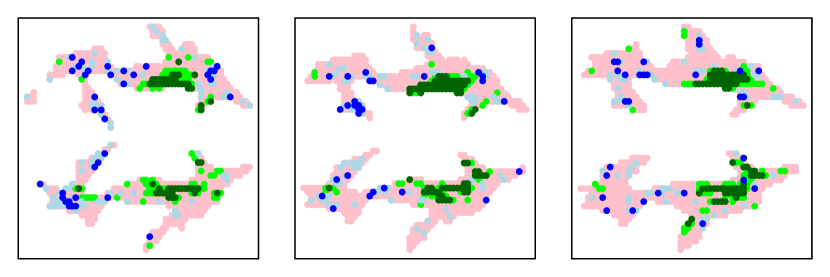
Figure 6: DTI $z$-scores at three adjacent vertical coordinates. Green and blue correspond to positive and negative values exceeding $z_{.975}$ in absolute value, and light green and light blue correspond to values exceeding $z_{.9}$ in absolute value.

The data exhibit a high degree of positive spatial dependence, with the $z$-values of neighboring voxels frequently being of the same sign. Also note that the spatial dependence among the large negative values appears to be much smaller than that of the large positive values, suggesting that many of the large negative values are due to noise.

Possible causes of this dependence include spatially dependent measurement errors and spatially structured signals. While it is likely that both of these factors are contributing to the spatial dependence, for the purpose of illustrating the SHPP we assume that it is exclusively the latter. We model these data as $z\sim N_{p}(\theta,I)$, and use a spatial SHPP for estimating $\theta$. Specifically, we write $\theta=u\circ v$ and optimize

$$g(u,v)=||z-u\circ v||^{2}+u^{\top}\Sigma^{-1}u+v^{\top}\Sigma^{-1}v,$$ (8)

where $\Sigma$ is the covariance matrix of a spatial conditional autoregression (CAR) model. The CAR model is parametrized as $\Sigma=\tau^{2}(I-\rho G)^{-1}$, where $\rho$ and $\tau^{2}$ are parameters and $G$ is a matrix of spatial weights. Letting $n_{i}$ be the number of voxels spatially adjacent to voxel $i$, the weights are given by $g_{i,j}=1/n_{i}$ if $j$ is adjacent to $i$ and $g_{i,j}=0$ otherwise. Under this model, the conditional expectation of $u_{i}$ given $\{u_{j}:j\neq i\}$ is $\rho$ times the average value of its neighbors, and the conditional variance is $\tau^{2}$.

Empirical Bayes estimates of $\rho$ and $\tau^{2}$ were obtained from the data and then used to define the SHPP objective function (8). To avoid calculations involving the $15,443\times 15,433$ covariance matrix $\Sigma$ that are necessary for the algorithm described above, we instead use a block coordinate descent algorithm that iteratively updates the values of $u_{i}$ and $v_{i}$ for each voxel $i$ as follows:

1. Compute $q=v_{i}^{2}+1/\tau^{2}$ and $l=z_{i}v_{i}+\rho\bar{u}_{n_{i}}/\tau^{2}$. Set $u_{i}=l/q$;

2. Compute $q=u_{i}^{2}+1/\tau^{2}$ and $l=z_{i}u_{i}+\rho\bar{v}_{n_{i}}/\tau^{2}$. Set $v_{i}=l/q$.

In the above algorithm, $\bar{u}_{n_{i}}$ denotes the average of the $u$-values among the $n_{i}$ neighbors of voxel $i$, and $\bar{v}_{n_{i}}$ is defined analogously. Starting with values of $u_{i}=|z_{i}|$ and $v_{i}=z_{i}/|z_{i}|$, this algorithm was iterated until the relative change in $u\circ v$ from one complete iteration over all voxels to the next was less than $10^{-10}$. This required 123 iterations and a little under two minutes on my desktop computer. The resulting estimate $\hat{\theta}$ is very sparse, with about 94% of the entries being less than $10^{-6}$ in absolute value (10 times smaller than the smallest entry of $z$). As shown in the top row of Figure 7, this sparsity is highly spatially structured, and a few large multi-voxel regions of the brain with consistently positive values are identified. The lack of non-zero negative values of $\hat{\theta}$ is in agreement with an analysis by Efron (2010, chapter 4) using false discovery rates, and further suggests that the few large and negative raw-data values at spatially isolated voxels are the result of noise. For comparison, the second row of the figure summarizes an unstructured lasso estimate, where the shrinkage parameter $\lambda$ was obtained using the same empirical Bayes approach described in Section 2.2. The unstructured estimate has non-zero negative values for several spatially isolated voxels, and the estimated positive regions are not as spatially coherent as those of the SHPP estimate.

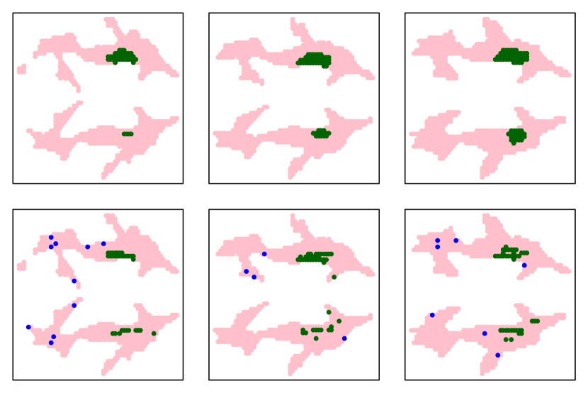
Figure 7: Estimated group differences using spatially structured (top) and unstructured (bottom) penalties. Green, blue and pink correspond to estimates that are positive, negative and zero respectively.

5 Discussion

The Hadamard product parametrization provides a simple and intuitive method for obtaining $L_{q}$-penalized regression estimates for certain values of $q$. In terms of accessibility to practitioners, the HPP algorithm is similar to the LQA algorithm. Both of these algorithms proceed by iterative ridge regression. Unlike the “ridge” of the LQA algorithm, that of the HPP algorithm is bounded near zero, suggesting that HPP is to be preferred over LQA for reasons of numerical stability. However, for the numerical examples in this article (and others considered by the author), instability was not an insurmountable issue for LQA and the two algorithms performed comparably.

The HPP algorithm updates only non-sparse parameter values, meaning that its computational costs are greatly reduced when the parameter values are highly sparse. Sparsity in parameter values can be introduced by combining HPP with a cyclic coordinate descent (CCD) algorithm. In a simulation study with a large number of predictors ($p=1000$), the resulting hybrid algorithm exhibited extremely fast convergence relative to standard CCD. However, in non-sparse high-dimensional scenarios, HPP as presented here may be impractical as it requires a Cholesky factorization at each iteration. One possible modification of HPP for such cases would be to use a first-order method (e.g. gradient descent) to do the optimization at each iteration.

The $L_{2}$ penalties on the parameters in the HPP can be thought of as isotropic normal prior distributions. Similarly, non-isotropic quadratic penalties can be constructed that can be interpreted as Gaussian models for the parameters. Such penalties can be useful in situations where the relationships between the parameters are naturally expressed in terms of a covariance model. However, the analogy to Bayesian estimation is limited: The value $(\hat{u},\hat{v})$ that minimizes $||y-X(u\circ v)||^{2}+\lambda(||u||^{2}+||v||^{2})/2$ is the posterior mode of $(u,v)$ under isotropic Gaussian priors, but $\hat{\beta}=\hat{u}\circ\hat{v}$ is not the posterior mode of $\beta$ under the prior induced by the Gaussian priors on $u$ and $v$. This is because, in general, the posterior mode of a function of a parameter is not the function at the posterior mode of the parameter. If $u$ and $v$ are a priori Gaussian then the induced prior distribution on $\beta$ is not a Laplace distribution (which would yield the Lasso estimate as a posterior mode), but a “normal product” distribution (Weisstein, 2016). This prior, considered by Zhou et al. (2015), corresponds to a different penalty than any of the $L_{q}$ penalties, and can be shown to be in the class of normal-gamma prior distributions studied by Griffin and Brown (2010).

Replication code for the numerical examples in this article is available at my website. I thank Panos Toulis for a helpful discussion. This research was supported by NSF grant DMS-1505136.

References

- Deutsch et al. (2005) Deutsch, G. K., R. F. Dougherty, R. Bammer, W. T. Siok, J. Gabrieli, and B. Wandell (2005). Correlations between white matter microstructure and reading performance in children. Cortex 41(3), 354–363.
- Efron (2010) Efron, B. (2010). Large-scale inference, Volume 1 of Institute of Mathematical Statistics (IMS) Monographs. Cambridge University Press, Cambridge. Empirical Bayes methods for estimation, testing, and prediction.
- Fan and Li (2001) Fan, J. and R. Li (2001). Variable selection via nonconcave penalized likelihood and its oracle properties. J. Amer. Statist. Assoc. 96(456), 1348–1360.
- Figueiredo (2003) Figueiredo, M. A. T. (2003, September). Adaptive sparseness for supervised learning. IEEE Trans. Pattern Anal. Mach. Intell. 25(9), 1150–1159.
- Friedman et al. (2010) Friedman, J., T. Hastie, and R. Tibshirani (2010). Regularization paths for generalized linear models via coordinate descent. Journal of Statistical Software 33(1), 1–22.
- Fu (1998) Fu, W. J. (1998). Penalized regressions: the bridge versus the lasso. J. Comput. Graph. Statist. 7(3), 397–416.
- Goeman et al. (2016) Goeman, J. J., R. J. Meijer, and N. Chaturvedi (2016). Penalized: L1 (lasso and fused lasso) and L2 (ridge) penalized estimation in GLMs and in the Cox model. R package version 0.9-47.
- Griffin and Brown (2010) Griffin, J. E. and P. J. Brown (2010). Inference with normal-gamma prior distributions in regression problems. Bayesian Anal. 5(1), 171–188.
- Hunter and Li (2005) Hunter, D. R. and R. Li (2005). Variable selection using MM algorithms. Ann. Statist. 33(4), 1617–1642.
- Kabán (2013) Kabán, A. (2013). Fractional norm regularization: Learning with very few relevant features. IEEE transactions on neural networks and learning systems 24(6), 953–963.
- Kabán and Durrant (2008) Kabán, A. and R. J. Durrant (2008). Learning with vs -norm regularisation with exponentially many irrelevant features. In Joint European Conference on Machine Learning and Knowledge Discovery in Databases, pp. 580–596. Springer.
- Luenberger and Ye (2008) Luenberger, D. G. and Y. Ye (2008). Linear and nonlinear programming (Third ed.). International Series in Operations Research & Management Science, 116. Springer, New York.
- Majindar (1963) Majindar, K. N. (1963). On a factorisation of positive definite matrices. Canad. Math. Bull. 6, 405–407.
- Park and Casella (2008) Park, T. and G. Casella (2008). The Bayesian lasso. J. Amer. Statist. Assoc. 103(482), 681–686.
- Schmidt et al. (2007) Schmidt, M., G. Fung, and R. Rosales (2007). Fast optimization methods for l1 regularization: A comparative study and two new approaches. In European Conference on Machine Learning, pp. 286–297. Springer.
- Styan (1973) Styan, G. P. H. (1973). Hadamard products and multivariate statistical analysis. Linear Algebra and Appl. 6, 217–240.
- Tibshirani (1996) Tibshirani, R. (1996). Regression shrinkage and selection via the lasso. J. Roy. Statist. Soc. Ser. B 58(1), 267–288.
- Tibshirani et al. (2005) Tibshirani, R., M. Saunders, S. Rosset, J. Zhu, and K. Knight (2005). Sparsity and smoothness via the fused lasso. J. R. Stat. Soc. Ser. B Stat. Methodol. 67(1), 91–108.
- Tibshirani (2013) Tibshirani, R. J. (2013). The lasso problem and uniqueness. Electron. J. Stat. 7, 1456–1490.
- Weisstein (2016) Weisstein, E. W. (2016). Normal product distribution. From MathWorld–A Wolfram Web Resource. Visited on 10/25/16.
- Yuan and Lin (2006) Yuan, M. and Y. Lin (2006). Model selection and estimation in regression with grouped variables. J. R. Stat. Soc. Ser. B Stat. Methodol. 68(1), 49–67.
- Zhou et al. (2015) Zhou, Z., K. Liu, and J. Fang (2015). Bayesian compressive sensing using normal product priors. IEEE Signal Processing Letters 22(5), 583–587.
- Zou and Li (2008) Zou, H. and R. Li (2008). One-step sparse estimates in nonconcave penalized likelihood models. Ann. Statist. 36(4), 1509–1533.