NNLL resummation for the associated production of a top pair and a Higgs boson at the LHC

Abstract

We study the resummation of soft gluon emission corrections to the production of a top-antitop pair in association with a Higgs boson at the Large Hadron Collider. Starting from a soft-gluon resummation formula derived in previous work, we develop a bespoke parton-level Monte Carlo program which can be used to calculate the total cross section along with differential distributions. We use this tool to study the phenomenological impact of the resummation to next-to-next-to-leading logarithmic (NNLL) accuracy, finding that these corrections increase the total cross section and the differential distributions with respect to NLO calculations of the same observables.

1 Introduction

The associated production of a top-quark pair and a Higgs boson can provide direct information on the Yukawa coupling of the Higgs boson to the top quark, which is crucial for verifying the origin of fermion masses and may shed light on the hierarchy problem related to the mass of the Higgs boson. For this reason, experimental collaborations at the Large Hadron Collider (LHC) are actively searching for this Higgs-boson production mode in the currently ongoing Run II. The Standard Model (SM) cross section for this process at a center-of-mass energy of $13$ TeV is quite small, of the order of $0.5$ pb.

Differences between the measured cross section and the corresponding SM predictions could indicate the presence of new physics which modifies the top-quark Yukawa coupling. Consequently, a large amount of work has been devoted to the study of this process beyond leading order (LO) in the SM. The LO cross section scales as $\alpha_{s}^{2}\alpha$, where $\alpha_{s}$ and $\alpha$ denote the strong coupling constant and the electromagnetic fine structure constant, respectively. The next-to-leading order (NLO) QCD corrections to this process were first evaluated more than ten years ago Beenakker:2001rj ; Beenakker:2002nc ; Reina:2001bc ; Reina:2001sf ; Dawson:2002tg ; Dawson:2003zu . This process also served as a benchmark for validating automated tools for NLO calculations; in Frederix:2011zi ; Garzelli:2011vp the NLO corrections were calculated automatically and interfaced with Monte Carlo event generators, thus including parton shower and hadronization effects. Electroweak corrections to this process were studied in Yu:2014cka ; Frixione:2014qaa ; Frixione:2015zaa . NLO QCD and electroweak corrections were included in the POWHEG framework in Hartanto:2015uka . In Denner:2015yca the NLO corrections to the associated production of a top pair and a Higgs boson were studied by considering also the decay of the top quark and off-shell effects. The cross section for the associated production of a top pair, a Higgs boson and an additional jet at NLO was evaluated in vanDeurzen:2013xla .

Perturbative calculations for the $t\bar{t}H$ production process are difficult and involved, due to the presence of five external legs, four of which carry color charges. Consequently, it is not likely that the next-to-next-to-leading order (NNLO) QCD corrections for this process will be computed in the near future. For this reason, the impact of soft gluon emission corrections beyond NLO was the subject of recent studies. In Kulesza:2015vda the soft gluon emission corrections to the total $t\bar{t}H$ cross section in the production threshold limit were evaluated up to next-to-leading logarithmic (NLL) accuracy; the production threshold is defined as the kinematic region in which the partonic center-of-mass energy approaches $2m_{t}+m_{H}$, which is the minimal energy of the final state. In Broggio:2015lya , on the other hand, we applied Soft-Collinear Effective Theory (SCET) methods in order to study the impact of soft-gluon corrections to the associated production of a top pair and a Higgs boson in the partonic threshold limit, i.e. in the limit where the partonic center-of-mass energy approaches the invariant mass $M$ of the $t\bar{t}H$ final state. The mass $M$ is bounded from above only by the hadronic center-of-mass energy. In Broggio:2015lya a resummation formula for the soft emission corrections was derived and all of the elements necessary for the evaluation of that formula to next-to-next-to-leading logarithmic (NNLL) accuracy were evaluated. By using these results, a study of the approximate NNLO corrections originating from soft gluon emission in the partonic threshold limit was carried out. In particular, an in-house parton level Monte Carlo program was developed and employed to evaluate the total cross section and several differential distributions. However, a direct numerical evaluation of the soft gluon emission corrections to NNLL was not performed in Broggio:2015lya . Recently, results for the total cross section and invariant mass distribution at NLL accuracy in the partonic threshold limit were presented in Kulesza:2016vnq .

From the technical point of view, the associated production of a top pair and a W boson shows several similarities to the associated production of a top pair and a Higgs boson. However, the former process involves only one partonic production channel in the partonic threshold limit, namely the quark annihilation channel, while the latter also receives large contributions from the gluon fusion channel. For this reason some of us recently studied the resummation of the soft gluon corrections in the partonic threshold limit to $t\bar{t}W$ production Broggio:2016zgg . In that work the resummation was carried out up to NNLL accuracy in Mellin space. An in-house parton level Monte Carlo program for the numerical evaluation of the resummation formulas was developed and employed to obtain predictions for the total cross section and several differential distributions at the LHC operating at a center-of-mass energy of $8$ and $13$ TeV. (The NNLL resummation in the partonic threshold limit for $t\bar{t}W$ production in momentum space was studied in Li:2014ula .)

By building upon the results of Broggio:2015lya and Broggio:2016zgg , in this paper we study the resummation of soft gluon emission corrections to the associated production of a top-quark pair and a Higgs boson in Mellin space. We developed an in-house parton level Monte Carlo code which allows us to evaluate numerically soft emission corrections to this process up to NNLL accuracy. By matching these results with complete NLO calculations carried out with MadGraph5_aMC@NLO Alwall:2014hca (which we will indicate with MG5_aMC in the rest of this paper) we obtain predictions for the total cross section and several differential distributions which are valid to NLO+NNLL accuracy. We also compute the observables at NLO+NLL accuracy and using NNLO approximations of the NLO+NNLL results, and show that these less precise computations miss important effects.

The paper is organized as follows: In Section 2 we review the salient features of the technique employed to obtain and evaluate the relevant resummation formulas. In Section 3 we present predictions, valid to NLO+NNLL accuracy, for the total cross section and several differential distributions for the associated production of a top pair and a Higgs boson at the LHC operating at a center-of-mass energy of $13$ TeV. Finally, Section 4 contains our conclusions.

2 Outline of the Calculation

The associated production of a top quark pair and a Higgs boson receives contributions from the partonic process

$$i(p_{1})+j(p_{2})\longrightarrow t(p_{3})+\bar{t}(p_{4})+H(p_{5})+X\,,$$ (1)

where $ij\in\{q\bar{q},\bar{q}q,gg\}$ at lowest order in QCD, and $X$ indicates the unobserved partonic final-state radiation. Two Mandelstam invariants play a crucial role in our discussion:

$$\hat{s}=(p_{1}+p_{2})^{2}=2p_{1}\cdot p_{2}\,,\quad\text{and}\quad M^{2}=\left(p_{3}+p_{4}+p_{5}\right)^{2}\,.$$ (2)

The soft or partonic threshold limit is defined as the kinematic situation in which

$$z\equiv\frac{M^{2}}{\hat{s}}\rightarrow 1\,.$$ (3)

In this region, the unobserved final state can contain only soft radiation.

The factorization formula for the QCD cross section in the partonic threshold limit was derived in Broggio:2015lya and reads

$$\sigma\left(s,m_{t},m_{H}\right)= \frac{1}{2s}\int_{\tau_{\text{min}}}^{1}\!\!\!d\tau\int^{1}_{\tau}\frac{dz}{\sqrt{z}}\sum_{ij}ff_{ij}\left(\frac{\tau}{z},\mu\right)$$

$$\times\int d\text{PS}_{t\bar{t}H}\mbox{Tr}\left[\mathbf{H}_{ij}\left(\{p\},\mu\right)\mathbf{S}_{ij}\left(\frac{M(1-z)}{\sqrt{z}},\{p\},\mu\right)\right]\,.$$ (4)

In (4), $s$ indicates the square of the hadronic center-of-mass energy and

$$\tau_{\text{min}}=\frac{\left(2m_{t}+m_{H}\right)^{2}}{s}\,,\qquad\tau=\frac{M^{2}}{s}\,.$$ (5)

We use the symbol $\{p\}$ to indicate the set of external momenta $p_{1},\cdots,p_{5}$. The trace $\mbox{Tr}\left[\mathbf{H}_{ij}\mathbf{S}_{ij}\right]$ is proportional to the spin and color averaged squared matrix element for $t\bar{t}H+X_{s}$ production in the process initiated by the two partons $i$ and $j$, where $X_{s}$ indicates the unobserved soft gluons in the final state. The hard functions $\mathbf{H}_{ij}$, which are matrices in color space, are obtained from the color decomposed virtual corrections to the $2\to 3$ tree-level process. The soft functions $\mathbf{S}_{ij}$ (which are also matrices in color space) are related to color-decomposed real emission corrections in the soft limit; they depend on plus distributions of the form

$$P^{\prime}_{n}(z)\equiv\left[\frac{1}{(1-z)}\ln^{n}\left(\frac{M^{2}(1-z)^{2}}{\mu^{2}z}\right)\right]_{+}\,,$$ (6)

as well as on the Dirac delta function of argument $(1-z)$. The parton luminosity functions $ff_{ij}$ are defined as the convolutions of the parton distribution functions (PDFs) for the partons $i$ and $j$ in the protons $N_{1}$ and $N_{2}$:

$$ff_{ij}\left(y,\mu\right)=\int_{y}^{1}\frac{dx}{x}f_{i/N_{1}}\left(x,\mu\right)f_{j/N_{2}}\left(\frac{y}{x},\mu\right)\,.$$ (7)

In the soft limit the indices $ij\in\{q\bar{q},\bar{q}q,gg\}$, as at LO. The hard and soft functions are two-by-two matrices for $q\bar{q}$-initiated (quark annihilation) processes, and three-by-three matrices for $gg$-initiated (gluon fusion) processes. Contributions from other production channels such as $\bar{q}g$ and $qg$ are subleading in the soft limit. We shall refer to such processes collectively as the “quark-gluon” or the “$qg$” channel in what follows.

The hard functions satisfy renormalization group equations governed by the soft anomalous dimension matrices $\mathbf{\Gamma}^{ij}_{H}$, which depend on the partonic channel considered. These anomalous dimension matrices, which are needed to carry out the resummation of soft gluon corrections, were derived in Ferroglia:2009ep ; Ferroglia:2009ii . The hard functions, soft functions, and soft anomalous dimensions must be computed in fixed-order perturbation theory up to a given order in $\alpha_{s}$. In this work we study the resummation up to NNLL accuracy. For this task we need to evaluate the hard functions, soft functions and soft anomalous dimensions to NLO. All of these elements were already evaluated to the order needed here Ferroglia:2009ep ; Ferroglia:2009ii ; Ahrens:2010zv ; Broggio:2015lya . In particular, the NLO hard functions were evaluated by customizing two of the one-loop provider programs available on the market, GoSam Cullen:2011ac ; Cullen:2014yla ; Binoth:2008uq ; Mastrolia:2010nb ; Peraro:2014cba and Openloops Cascioli:2011va . The numerical evaluation of the hard functions for this work has been performed by using a modified version of Openloops in combination with Collier Denner:2002ii ; Denner:2005nn ; Denner:2010tr ; Denner:2014gla ; Denner:2016kdg . GoSam in combination with Ninja Peraro:2014cba ; Mastrolia:2012bu ; vanDeurzen:2013saa was used to cross-check our results.

The resummation formula for the associated production of a $t\bar{t}H$ final state in Mellin space is similar to the one which was derived for the production of a $t\bar{t}W$ final state in Broggio:2016zgg and reads

$$\sigma(s,m_{t},m_{H})= \frac{1}{2s}\int_{\tau_{\text{min}}}^{1}\frac{d\tau}{\tau}\frac{1}{2\pi i}\int_{c-i\infty}^{c+i\infty}dN\tau^{-N}\sum_{ij}\widetilde{ff}_{ij}\left(N,\mu\right)\int d\text{PS}_{t\bar{t}H}\,\widetilde{c}_{ij}\left(N,\mu\right)\,,$$ (8)

where we introduced the Mellin transform of the luminosity functions $\widetilde{ff}_{ij}$, and

$$\widetilde{c}_{ij}\left(N,\mu\right)\equiv\mbox{Tr}\left[\mathbf{H}_{ij}\left(\{p\},\mu\right)\mathbf{\widetilde{s}}_{ij}\left(\ln\frac{M^{2}}{\bar{N}\mu^{2}},\{p\},\mu\right)\right]\,.$$ (9)

Since the soft limit $z\to 1$ corresponds to the limit $N\to\infty$ in Mellin space, we neglected terms suppressed by powers of $1/N$ in (8). Furthermore, in (9) we employed the notation $\bar{N}=Ne^{\gamma_{E}}$. The function $\mathbf{\widetilde{s}}_{ij}$ is the Mellin transform of the soft function $\mathbf{S}_{ij}$ found in (4).

The hard and soft functions in (8) can be evaluated in fixed order perturbation theory at scales at which they are free from large logarithms. We indicate these scales with $\mu_{h}$ and $\mu_{s}$, respectively. Subsequently, by solving the renormalization group (RG) equations for the hard and soft functions one can evolve the hard scattering kernels in (9) to the factorization scale $\mu_{f}$. One obtains

$$\widetilde{c}_{ij}(N,\mu_{f})=\mbox{Tr}\Bigg{[} \widetilde{\mathbf{U}}_{ij}(\!\bar{N},\{p\},\mu_{f},\mu_{h},\mu_{s})\,\mathbf{H}_{ij}(\{p\},\mu_{h})\,\widetilde{\mathbf{U}}_{ij}^{\dagger}(\!\bar{N},\{p\},\mu_{f},\mu_{h},\mu_{s})$$

$$\times\widetilde{\mathbf{s}}_{ij}\left(\ln\frac{M^{2}}{\bar{N}^{2}\mu_{s}^{2}},\{p\},\mu_{s}\right)\Bigg{]}\,.$$ (10)

Large logarithmic corrections depending on the ratio of the scales $\mu_{h}$ and $\mu_{s}$ are resummed in the channel-dependent matrix-valued evolution factors $\widetilde{\mathbf{U}}$. The expression for the evolution factors is

$$\widetilde{\mathbf{U}}\left(\bar{N},\{p\},\mu_{f},\mu_{h},\mu_{s}\right)= \exp\Biggl{\{}2S_{\Gamma_{\text{cusp}}}(\mu_{h},\mu_{s})-a_{\Gamma_{\text{cusp}}}(\mu_{h},\mu_{s})\ln\frac{M^{2}}{\mu_{h}^{2}}+a_{\Gamma_{\text{cusp}}}(\mu_{f},\mu_{s})\ln\bar{N}^{2}$$

$$+2a_{\gamma^{\phi}}(\mu_{s},\mu_{f})\Biggr{\}}\times\mathbf{u}\left(\{p\},\mu_{h},\mu_{s}\right),$$ (11)

which is formally identical to the expression found for the corresponding quantity in carrying out the resummation for $t\bar{t}W$ production. For the definition of the various RG factors appearing in (11) we refer the reader to Broggio:2016zgg . However, while for $t\bar{t}W$ production one needs to consider the evolution factor in the quark-annihilation channel only, for $t\bar{t}H$ production one also needs to evaluate the appropriate anomalous dimensions and evolution factor for the gluon fusion channel.

The functions $\mathbf{U}$ in (11) depend on $\alpha_{s}$ evaluated at three different scales: $\mu_{h}$, $\mu_{s}$ and $\mu_{f}$. In practice, it is convenient to rewrite the evolution factors in terms of $\alpha_{s}(\mu_{h})$ only. This can be done by employing the running of $\alpha_{s}$ at three loops Moch:2005ba . By doing this, logarithms such as $\ln(\mu_{h}/\mu_{s})$ appear explicitly in the formula for the evolution matrix, which becomes Broggio:2016zgg

$$\widetilde{\mathbf{U}}\left(\bar{N},\{p\},\mu_{f},\mu_{h},\mu_{s}\right)= \exp\Biggl{\{}\frac{4\pi}{\alpha_{s}(\mu_{h})}g_{1}\left(\lambda,\lambda_{f}\right)+g_{2}\left(\lambda,\lambda_{f}\right)+\frac{\alpha_{s}(\mu_{h})}{4\pi}g_{3}\left(\lambda,\lambda_{f}\right)+\cdots\Biggr{\}}$$

$$\times\mathbf{u}(\{p\},\mu_{h},\mu_{s})\,,$$ (12)

with

$$\lambda=\frac{\alpha_{s}(\mu_{h})}{2\pi}\beta_{0}\ln{\frac{\mu_{h}}{\mu_{s}}}\,,\qquad\lambda_{f}=\frac{\alpha_{s}(\mu_{h})}{2\pi}\beta_{0}\ln{\frac{\mu_{h}}{\mu_{f}}}\,.$$ (13)

The leading logarithmic (LL) function $g_{1}$, the NLL function $g_{2}$, and the NNLL function $g_{3}$ can be obtained starting from (11). One can see that the l.h.s of (10) is independent of $\mu_{h}$ and $\mu_{s}$ if the evolution factors and the hard and soft functions are known to all orders in perturbation theory. This is impossible in practice, which introduces a residual dependence on the choice of the scales $\mu_{h}$ and $\mu_{s}$ in any numerical evaluation of (11) or (12). The hard and soft functions are free from large logarithms if one chooses $\mu_{h}\sim M$ and $\mu_{s}\sim M/\bar{N}$. It is well known that one then faces the presence of a branch cut for large values of $N$ in the hard scattering kernel, whose existence is related to the Landau pole in $\alpha_{s}$. In this work, we choose the integration path in the complex $N$ plane when evaluating the inverse Mellin transform according to the Minimal Prescription (MP) introduced in Catani:1996yz . In the numerics, we need the parton luminosity functions in Mellin space. These can be constructed using techniques described in Bonvini:2012sh ; Bonvini:2014joa .

3 Numerical Results

$M_{W}$	$80.419$ GeV	$m_{t}$	$173.2$ GeV
$M_{Z}$	$91.1876$ GeV	$m_{H}$	$125$ GeV
$G_{F}$	$1.16639\times 10^{-5}$ GeV-2	$\alpha_{s}\left(M_{Z}\right)$	from MMHT 2014 PDFs

Table 1: Input parameters employed throughout the calculation.

In this section we present predictions for the total cross section and differential distributions for the $t\bar{t}H$ production process. The main goal of this work is to obtain predictions for physical observables which are valid to NLO+NNLL accuracy. However, we also perform some systematic studies meant to provide insight into the validity of various approximations to this state-of-the-art result. In all cases, we use the input parameters listed in Table 1, and MMHT 2014 PDFs Harland-Lang:2014zoa . We switch PDF orders as appropriate for a given perturbative approximation according to the scheme given in Table 2, where we also specify the computer code used in each case.

As a preliminary step we check that with our choice of scales and input parameters the NLO expansion of the NNLL resummation formula (which we refer to as “approximate NLO”) provides a satisfactory approximation to the exact NLO calculation. Such an approximation of (10) captures the leading terms in the Mellin-space soft limit ($N\to\infty$) of the NLO cross section, namely the single and double powers of $\ln N$ as well as $N$-independent terms. Even though the $N$-independent terms depend on the Mandelstam variables, we will refer to them as “constant” terms in what follows. Analogous comparisons of approximate NLO and complete NLO calculations were carried out for $t\bar{t}W$ production in Broggio:2016zgg . In Broggio:2015lya , similar comparisons were also performed for $t\bar{t}H$ production, but with two differences with respect to the current work: the renormalization and factorization scales were fixed (independent of $M$) instead of dynamic (correlated with $M$), and the leading terms were represented in momentum space instead of Mellin space.

The NLO approximation mentioned above is easily obtained by setting $\mu_{s}=\mu_{h}=\mu_{f}$ in the NNLL resummation formula (10). For this reason, the matched NLO+NNLL cross section is given by

$$\sigma^{{\text{NLO+NNLL}}}= \sigma^{{\text{NLO}}}+\left[\sigma^{\text{NNLL}}-\sigma^{\text{approx. NLO}}\right]\,.$$ (14)

The difference of terms in the square brackets contributes at NNLO and beyond, adding NNLL resummation onto the NLO result. In order to study the convergence of resummed perturbation theory, we will also calculate NLO+NLL results, defined as

$$\sigma^{{\text{NLO+NLL}}}= \sigma^{{\text{NLO}}}+\left[\sigma^{{\text{NLL}}}-\sigma^{{\text{NLL expanded to NLO}}}\right]\,.$$ (15)

The difference of terms in the square brackets contributes at NNLO and beyond, adding NLL resummation onto the NLO result. However, in contrast to the approximate NLO result, the constant piece of the NLO expansion of the NLL resummation formula contains explicit dependence on the matching scales $\mu_{h}$ and $\mu_{s}$, in addition to that on $\mu_{f}$. The numerical dependence on these scales is formally of NNLL order (and is indeed canceled through $\mu_{s}$ and $\mu_{h}$ dependence in the NLO hard and soft functions in the NNLL result), and provides an additional handle on estimating the size of NNLL corrections using the NLL resummation formula.

While we are mainly interested in NNLL resummation effects, it is also interesting to study to what extent these all-orders corrections are approximated by their NNLO truncation. To this end, we consider “approximate NNLO” calculations based on the NNLL resummation formula (10). Approximate NNLO calculations include all powers of $\ln N$ and part of the constant terms from a complete NNLO calculation, but neglect terms which vanish as $N\to\infty$. Since the constant terms are not fully determined by an NNLL calculation (only their $\mu$-dependence is, through the RG equations), there is some freedom as to how to construct such approximations.

Here we consider two possibilities. The first follows the procedure used in Broggio:2016zgg for the case of $t\bar{t}W$ production. A detailed description of which constant pieces are included in that NNLO approximation can be found in Section 4 of Broggio:2016zgg . We match these NNLO corrections, obtained in the soft limit, with the NLO ones in the usual way:

$$\sigma^{\text{nNLO}}=\sigma^{\text{NLO}}+\left[\sigma^{\text{approx. NNLO}}-\sigma^{\text{approx. NLO}}\right]\,,$$ (16)

where we introduced the acronym nNLO to indicate approximate NNLO corrections matched to full NLO calculations. The second NNLO approximation we consider is based on the direct expansion of the NLO+NNLL result to NNLO. This differs from the approximate NNLO result used above by constant terms, which are formally of N³LL order. We define this approximation through the matching equation

$$\left(\sigma^{\text{NLO+NNLL}}\right)_{\text{NNLO exp.}} =\sigma^{\text{NLO}}+\left[\sigma^{\text{NNLL expanded to NNLO}}-\sigma^{\text{approx. NLO}}\right]\,.$$ (17)

In both cases above, the difference of terms in the square brackets is a pure NNLO correction. Contrary to the approximate NNLO result used in (16), which depends only on $\mu_{f}$ by construction, the constant pieces of the NNLO expansion of the NNLL result in (17) contain explicit dependence on $\mu_{h}$ and $\mu_{s}$, in addition to that on $\mu_{f}$. This scale dependence is formally of N³LL order, and can be used to estimate the size of such corrections to the NNLL results. Moreover, the NNLO approximation (17) differs from the NLO+NNLL result through terms of N³LO and higher, so comparing the two results gives a direct measure of how important such terms are numerically. In fact, were an exact NNLO calculation to appear, adding to it these beyond NNLO terms would achieve NNLO+NNLL resummation.

3.1 Scale choices

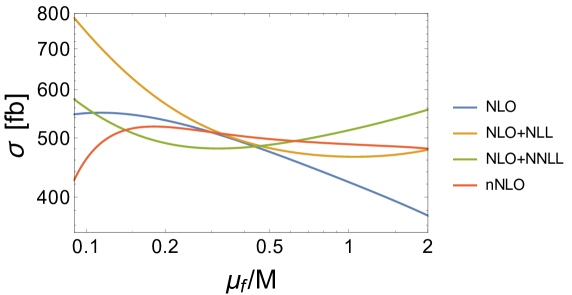
Figure 1: Factorization-scale dependence of the total $t\bar{t}H$ production cross section at the LHC with $\sqrt{s}=13$ TeV. The NLO and NLO+NLL curves are obtained using MMHT 2014 NLO PDFs, while the NLO+NNLL and nNLO curves are obtained using MMHT 2014 NNLO PDFs.

Numerical evaluations of the resummed formulas have a residual dependence on the choice of the hard and soft scales $\mu_{h}$ and $\mu_{s}$. This feature arises from the fact that the various factors in (10) have to be evaluated at a given order in perturbation theory. When the resummation is carried out in Mellin space the standard default choice of these scales is $\mu_{h,0}=M$ and $\mu_{s,0}=M/\bar{N}$ Ferroglia:2015ivv ; Pecjak:2016nee ; Broggio:2016zgg . This choice is the same one followed in the “direct QCD” resummation method Catani:1996yz ; Bonvini:2012az ; Bonvini:2014qga , and is the one we shall use here.

Furthermore, both the fixed-order and resummed results have a residual dependence on the factorization scale $\mu_{f}$. The factorization scale should be chosen in such a way that logarithms of the ratio $\mu_{f}/M$ are not large Collins:1989gx . Since we are working in the partonic threshold limit it is natural to choose a dynamical value for the factorization scale which is correlated with the final state invariant mass $M$. Figure 1 shows the dependence of the total cross section calculated within various perturbative approximations on the choice of the ratio $\mu_{f}/M$ at the LHC with $\sqrt{s}=13$ TeV. One can observe that the NLO, NLO+NLL and NLO+NNLL curves intersect each other in the vicinity of $\mu_{f}/M=0.5$, while the three curves have a very different behavior for small values of $\mu_{f}$. In addition, Figure 1 shows that beyond-NLO corrections are quite significant for $\mu_{f}/M\gg 0.5$, as the NLO result falls rather steeply away to smaller values in that region, while the other three curves remain reasonably stable.

Because of these considerations, in the following we employ two different default choices for the factorization scale, namely $\mu_{f,0}=M/2$ and $\mu_{f,0}=M$. The choice $\mu_{f,0}=M/2$ may be advantageous because the lower-order perturbative results are larger at lower $\mu_{f}$, so that the apparent convergence of the perturbative series is improved, but other than this numerical fact there is no obvious reason to exclude the natural hard scale $M$ as a default choice so we study this as well. In both cases, the uncertainty associated to the choice of a default value for the scale is estimated by varying each scale in the interval $[\mu_{i,0}/2,2\mu_{i,0}]$ ($i\in\{s,f,h\}$). The scale uncertainty above the central value of an observable $O$ (the total cross section, or the value of a differential cross section in a given bin) is then evaluated by combining in quadrature the quantities

$$\Delta O_{i}^{+}=\text{max}\{O\left(\kappa_{i}=1/2\right),O\left(\kappa_{i}=1\right),O\left(\kappa_{i}=2\right)\}-\bar{O}\,,$$ (18)

for $i=f,h,s$. In (18) $\kappa_{i}=\mu_{i}/\mu_{i,0}$ and $\bar{O}$ is the value of $O$ evaluated by setting all scales to their default values ($\kappa_{i}=1$ for $i=f,h,s$). The scale uncertainty below the central value can be obtained in the same way by combining in quadrature the quantities $\Delta O_{i}^{-}$, defined as in (18) but with “max” replaced by “min”. We use this procedure to obtain the perturbative uncertainties given in all of the tables and figures that follow.

3.2 Total cross section

order	PDF order	code	$\sigma$ [fb]
LO	LO	MG5_aMC	$378.7^{+120.5}_{-85.2}$
app. NLO	NLO	in-house MC	$473.3^{+0.0}_{-28.6}$
NLO no $qg$	NLO	MG5_aMC	$482.1^{+10.9}_{-35.1}$
NLO	NLO	MG5_aMC	$474.8^{+47.2}_{-51.9}$
NLO+NLL	NLO	in-house MC +MG5_aMC	$480.1^{+57.7}_{-15.7}$
NLO+NNLL	NNLO	in-house MC +MG5_aMC	$486.4^{+29.9}_{-24.5}$
nNLO (Mellin)	NNLO	in-house MC +MG5_aMC	$497.9^{+18.5}_{-9.4}$
(NLO+NNLL)${}_{\rm NNLO\,exp.}$	NNLO	in-house MC +MG5_aMC	$482.7^{+10.7}_{-21.1}$

Table 2: Total cross section for $t\bar{t}H$ production at the LHC with $\sqrt{s}=13$ TeV and MMHT 2014 PDFs. The default value of the factorization scale is $\mu_{f,0}=M/2$, and the uncertainties are estimated through scale variations of this (and the resummation scales $\mu_{s}$ and $\mu_{h}$ when applicable) as explained in the text, see the discussion around (18).

We begin our analysis by considering the total cross section for the associated production of a top pair and a Higgs boson at the LHC operating at a center-of-mass energy of 13 TeV. The results obtained are summarized in Table 2, where we set $\mu_{f,0}=M/2$, in Table 3, where we set $\mu_{f,0}=M$, and in Figure 2, which presents a visual comparison between the main results at the two different scales.

We first compare the approximate NLO corrections generated from NNLL soft-gluon resummation (second row of each table), with the full NLO corrections without (third row of each table) and with (fourth row of each table) the $qg$ channel. Since the approximate NLO results include only the leading-power contributions from the gluon fusion and quark-annihilation channels in the soft limit, the difference between these results and the NLO corrections without the $qg$ channel gives a measure of the importance of power corrections away from this limit. The two results are seen to differ by no more than a few percent, even though the NLO corrections are large. This shows that at NLO the power corrections away from the soft limit for these channels are quite small. Comparing the NLO results with and without the $qg$ channel reveals that this channel contributes significantly to the scale uncertainty, in particular when one chooses $\mu_{f,0}=M/2$. The fact that the leading terms in the soft limit make up the bulk of the NLO correction provides a strong motivation to resum them to all orders. No information is lost by doing this, as both sources of power corrections are taken into account by matching with NLO as discussed above. Since the power corrections are treated in fixed order, the perturbative uncertainties associated with them are estimated through the standard approach of scale variations.

order	PDF order	code	$\sigma$ [fb]
LO	LO	MG5_aMC	$293.5^{+85.2}_{-61.7}$
app. NLO	NLO	in-house MC	$444.7^{+28.6}_{-39.2}$
NLO no $qg$	NLO	MG5_aMC	$447.0^{+35.1}_{-40.4}$
NLO	NLO	MG5_aMC	$423.0^{+51.9}_{-49.7}$
NLO+NLL	NLO	in-house MC +MG5_aMC	$466.2^{+22.9}_{-26.8}$
NLO+NNLL	NNLO	in-house MC +MG5_aMC	$514.3^{+42.9}_{-39.5}$
nNLO (Mellin)	NNLO	in-house MC +MG5_aMC	$488.4^{+9.4}_{-8.3}$
(NLO+NNLL)${}_{\rm NNLO\,exp.}$	NNLO	in-house MC +MG5_aMC	$485.7^{+6.8}_{-15.0}$

Table 3: Total cross section for $t\bar{t}H$ at the LHC with $\sqrt{s}=13$ TeV and MMHT 2014 PDFs. The results are obtained as in Table 2, but with the default value of the factorization scale chosen instead as $\mu_{f,0}=M$.

We next turn to the NLO+NLL and NLO+NNLL cross sections, which are the main results of this section. The exact numbers are given in Tables 2 and 3, and a pictorial representation is given in Figure 2. The results for the default scale choice $\mu_{f,0}=M/2$ converge quite nicely. The scale uncertainties get progressively smaller when moving from NLO to NLO+NLL to NLO+NNLL, and the higher-order results are roughly within the range predicted by the uncertainty bands of the lower-order ones. For $\mu_{f,0}=M$ the convergence is still reasonable but not quite as good, mainly because the NLO and NLO+NLL results are noticeably smaller than at $\mu_{f,0}=M/2$. Interestingly, the NLO+NLL result has a smaller scale uncertainty than the NLO+NNLL one for $\mu_{f,0}=M$, a fact which looks rather accidental considering its wider variation over a larger range of $\mu_{f}$, as seen in Figure 1. However, one should remember that the scales $\mu_{h}$ and $\mu_{s}$ are kept fixed at their default values in the NLO+NLL and NLO+NNLL curves of Figure 1, while they are varied as explained above in order to obtain the scale uncertainty reported in the tables.

Finally, we discuss the NNLO approximations to the NNLL resummation formula. The results in Table 2 show that for $\mu_{f,0}=M/2$ the importance of resummation effects beyond NNLO is rather small, roughly at or below the 5% level after taking scale uncertainties into account. An examination of Table 3 shows that the effects are noticeably larger at $\mu_{f,0}=M$, approximately at the 10% level. In either case, Figure 2 shows very clearly that the nNLO results display an artificially small scale dependence compared to the NLO+NNLL results, confirming the cautionary statements made in Broggio:2015lya about the reliability of the nNLO scale dependence in estimating higher-order perturbative corrections.

The results in this section highlight the importance of an NNLL calculation. Taken as a whole, they show that both NLO+NLL and approximate NNLO calculations are a poor proxy for the more complete NLO+NNLL calculation. We have considered two default scale choices, $\mu_{f,0}=M/2$ and $\mu_{f,0}=M$. However, we should emphasize that in the end the default scale choice is arbitrary, and it would not be unreasonable to combine the envelope of results from the two choices into a single, larger perturbative uncertainty. The NLO+NNLL results quoted at either scale would not change significantly through such a combination.

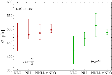
Figure 2: Comparison between different perturbative approximations to the total cross section carried out with the default factorization scale choices $\mu_{f,0}=M/2$ (left) and $\mu_{f,0}=M$ (right). The labels “NLL” and “NNLL” on the horizontal axis indicate NLO+NLL and NLO+NNLL calculations.

3.3 Differential distributions

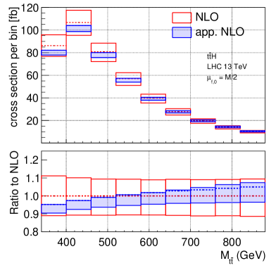
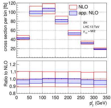
Figure 3: Differential distributions at approximate NLO (blue band) compared to the complete NLO (red band). The default factorization scale is chosen as $\mu_{f,0}=M/2$, and the uncertainty bands are generated through scale variations as explained in the text.

In this section we discuss results for differential distributions. In particular, we consider:

• the distribution differential with respect to the invariant mass of the top pair and Higgs boson in the final state, $M$;

• the distribution differential with respect to the invariant mass of the top-quark pair, $M_{t\bar{t}}$;

• the distribution differential with respect to the transverse momentum of the Higgs boson, $p_{T}^{H}$;

• the distribution differential with respect to the transverse momentum of the top quark, $p_{T}^{t}$.

We first set the default value of the factorization scale to $\mu_{f,0}=M/2$. Figure 3 shows the comparison between complete NLO calculations and approximate NLO calculations for all of the distributions listed above. We observe that for all of the distributions the approximate NLO scale uncertainty band (in blue) is included in the NLO scale uncertainty band (bins with the red frame). However, the approximate NLO uncertainty is smaller than the NLO uncertainty in all bins. Furthermore the bin-by-bin ratio of the two distributions, found at the bottom of each panel, shows that the NLO and approximate NLO corrections have somewhat different shapes.

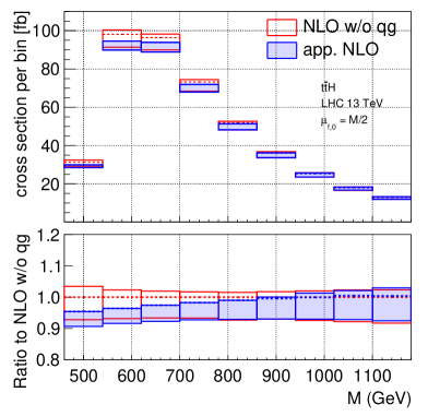
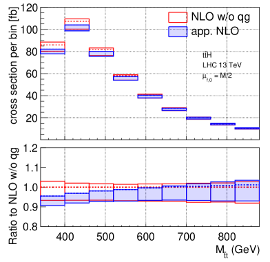
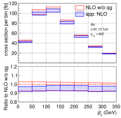
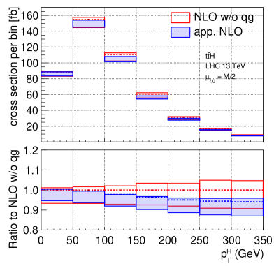
Figure 4: Differential distributions at approximate NLO (blue band) compared to the NLO distributions without the quark-gluon channel contribution (red band). All settings are as in Figure 3.

As for the case of the total cross section, it is reasonable to look at how the approximate NLO distributions compare to the NLO calculations when the contribution of the $qg$ channel is left out from the latter. This comparison can be found in Figure 4. One can see that approximate NLO and NLO distributions without the $qg$ channel agree quite well and the size of the respective uncertainty bands is very similar. We remind the reader that the contribution of the $qg$-channel at NLO is included in the NLO+NLL, NLO+NNLL and nNLO predictions discussed below through the matching procedure.

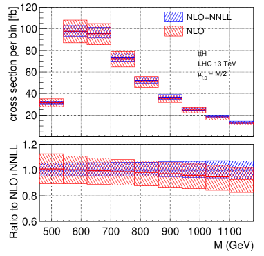
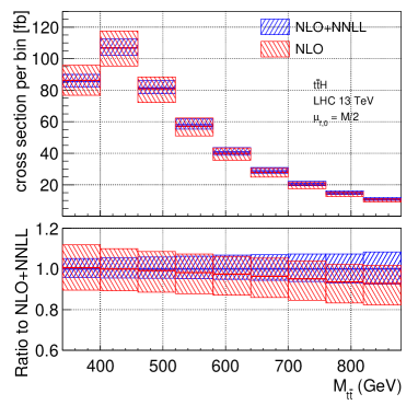
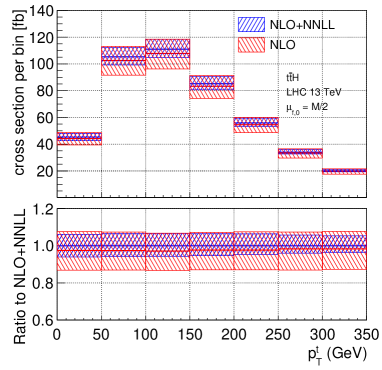
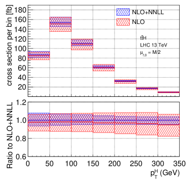
Figure 5: Differential distributions with $\mu_{f,0}=M/2$ at NLO+NNLL (blue band) compared to the NLO calculation (red band). The uncertainty bands are generated through scale variations of $\mu_{f}$, $\mu_{s}$ and $\mu_{h}$ as explained in the text.

The comparison between the NLO and the NLO+NNLL calculations of the differential distributions can be found in Figure 5. We see that the NLO+NNLL uncertainty band is included in the NLO scale uncertainty band in almost all bins of the distributions considered here. The exception is the bins in the far tail of the $M$ and $M_{t\bar{t}}$ distributions, where the NLO+NNLL band is not completely included in the NLO one, but is higher than the NLO one. In general one can observe that the central value of the NLO+NNLL calculation is slightly larger than the central value of the NLO one in almost all bins of the distributions shown in Figure 5.

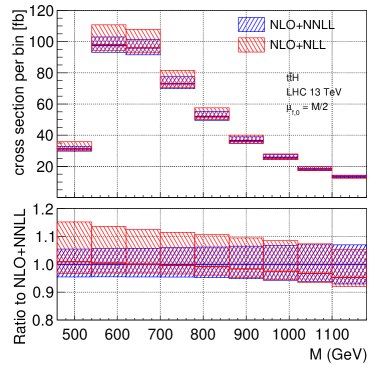
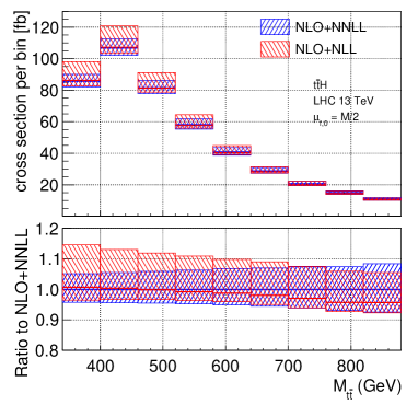
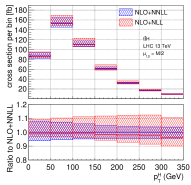
Figure 6: Differential distributions $\mu_{f,0}=M/2$ at NLO+NNLL (blue band) compared to the NLO+NLL calculation (red band). The uncertainty bands are generated through scale variations.

Figure 6 shows a comparison between NLO+NLL and NLO+NNLL results. The central value of these two calculations is quite close in all bins. The main effect of the corrections at NLO+NNLL is to shrink slightly the scale uncertainty bands with respect to the NLO+NLL results everywhere with the exception of the bins in the far tail of the $M$ and $M_{t\bar{t}}$ distributions.

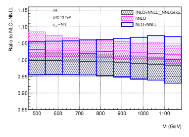
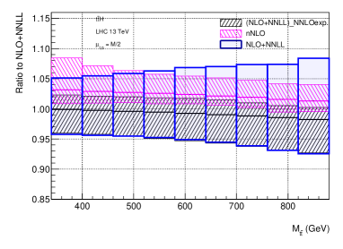
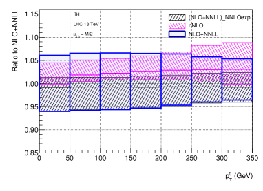
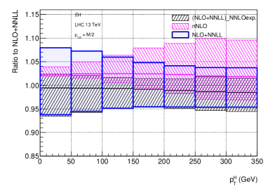
Figure 7: Differential distributions ratios for $\mu_{f,0}=M/2$, where the uncertainties are generated through scale variations.

We conclude our discussion of the results obtained with the choice $\mu_{f,0}=M/2$ by comparing in Figure 7 the NLO+NNLL, nNLO and NLO+NNLL expanded predictions for the various distributions. The figure shows the ratio, separately for each bin, of the distribution to the NLO+NNLL prediction evaluated with $\mu_{i}=\mu_{i,0}$ for $i=s,f,h$. The blue band refers to NLO+NNLL calculations, the dashed red band to nNLO calculations and the dashed black band to the NNLO expansion of the NLO+NNLL resummation. The dashed black band and the blue band thus differ by NNLL resummation effects of order N³LO and higher. Numerically, these effects contribute roughly at the 5% level, and as for the total cross section the NNLO truncation of the NLO+NNLL resummation formula tends to underestimate the uncertainty of the all-orders resummation. The difference between the dashed red band and the dashed black band is due to constant NNLO corrections, which are of N³LL order. Taking the envelope of the two NNLO approximations (i.e. the black and red bands) gives a more realistic estimate of the scale uncertainty, which is generally contained within the NLO+NNLL result (the exception is the high-$p_{T}^{H}$ bins).

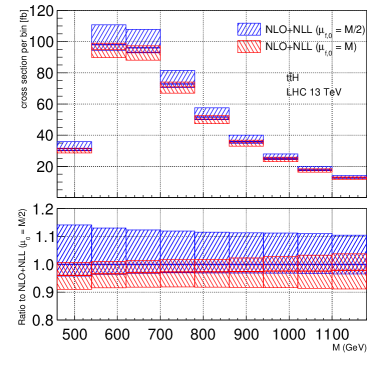
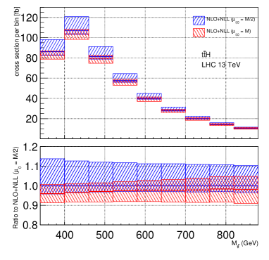
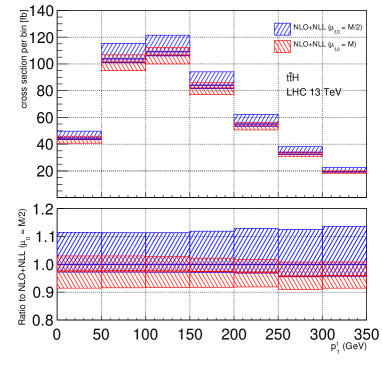
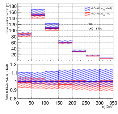
Figure 8: Differential distributions at NLO+NLL at $\mu_{f,0}=M/2$ (blue band) compared to the NLO+NLL calculation at $\mu_{f,0}=M$ (red band), where the uncertainties are generated through scale variations.

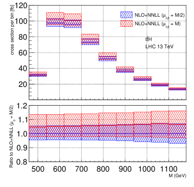
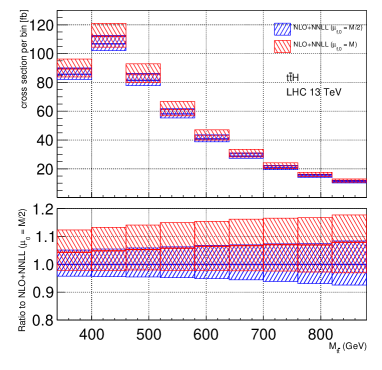
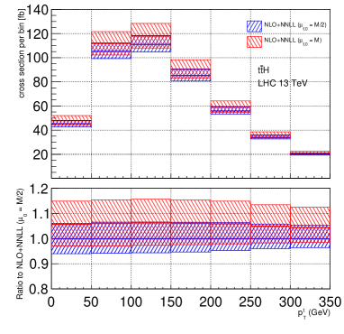
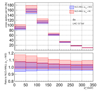
Figure 9: Differential distributions at NLO+NNLL at $\mu_{f,0}=M/2$ (blue band) compared to the NLO+NNLL calculation at $\mu_{f,0}=M$ (red band), where the uncertainties are generated through scale variations.

We want at this point to study results for a different choice of the default factorization scale, namely $\mu_{f,0}=M$. As discussed for the case of the total cross section in Section 3.2, the numerical impact of the soft emission corrections with the choice $\mu_{f,0}=M$ is significantly larger than the impact of the same corrections with the choice $\mu_{f,0}=M/2$. However, NLO+NNLL predictions obtained with the two choices are in good agreement. For what concerns the differential distributions studied here this can be seen by comparing NLO+NLL calculations carried out with the choice $\mu_{f,0}=M$ or $\mu_{f,0}=M/2$ (Figure 8), and NLO+NNLL calculations with $\mu_{f,0}=M$ or $\mu_{f,0}=M/2$ (Figure 9). Figure 8 shows that at NLO+NLL the overlap between the distributions evaluated at $\mu_{f,0}=M$ and $\mu_{f,0}=M/2$ is not particularly good, with the band at $\mu_{f,0}=M/2$ slightly larger than the one at $\mu_{f,0}=M$ in all bins. Figure 9 shows instead that the NLO+NNLL distributions at $\mu_{f,0}=M$ and $\mu_{f,0}=M/2$ have a large overlap in all bins. The scale uncertainty at NLO+NNLL with $\mu_{f,0}=M$ is larger than the scale uncertainty at $\mu_{f,0}=M/2$ in all bins. The good agreement between the two bands shown in each panel of Figure 9 indicates that NLO+NNLL predictions are quite stable with respect to different (but reasonable) choices of the standard value for the factorization scale.

4 Conclusions

In this paper we evaluated the resummation of the soft emission corrections to the associated production of a top-quark pair and a Higgs boson at the LHC in the partonic threshold limit $z\to 1$. The calculation is carried out to NNLL accuracy and it is matched to the complete NLO cross section in QCD. The numerical evaluation of observables at NLO+NNLL was carried out by means of an in-house parton level Monte Carlo code developed for this work, based on the resummation formula derived in Broggio:2015lya . The resummation procedure is however carried out in Mellin space, following the same approach employed in Ferroglia:2015ivv ; Pecjak:2016nee for the calculation of the (boosted) top-quark pair production cross section and in Broggio:2016zgg for the calculation of the cross section for the associated production of a top-quark pair and a $W$ boson.

In the previous sections we presented predictions for the total cross section for this production process at the LHC operating at a center-of-mass energy of $13$ TeV. In addition, we showed results for four different differential distributions depending on the four-momenta of the massive particles in the final state: the differential distributions in the invariant mass of the $t\bar{t}H$ particles, in the invariant mass of the $t\bar{t}$ pair, in the transverse momentum of the Higgs boson, and in the transverse momentum of the top quark. We found that the relative size of the NNLL corrections with respect to the NLO cross section is rather sensitive to the choice of the factorization scale $\mu_{f}$. In particular, for the two choices which we analyzed in detail, namely $\mu_{f,0}=M/2$ and $\mu_{f,0}=M$, it was found that the NNLL corrections enhance the total cross section and differential distributions in all bins considered. The NNLL soft emission corrections expressed as a percentage of the NLO observables are larger at $\mu_{f,0}=M$ than they are at $\mu_{f,0}=M/2$. However, by comparing NLO+NNLL predictions obtained by setting $\mu_{f,0}=M/2$ with NLO+NNLL predictions evaluated with $\mu_{f,0}=M$, and after accounting for the scale uncertainty affecting both predictions, we find compatible results. This fact shows that the NLO+NNLL predictions are quite stable with respect to the factorization scale choice. Indeed, it would not be unreasonable to combine the envelope of the results at the two different scale choices into a single result with a larger perturbative uncertainty, which for the case of the total cross section would be at about the 20 % level. By taking the envelope of the corresponding NLO results, one finds instead an uncertainty larger than 30 %. We also studied the total cross section and differential distributions at NLO+NLL accuracy and with NNLO approximations of the NLO+NNLL resummation formula, and found that both of these are a poor proxy for the more complete NLO+NNLL results, especially for higher values of $\mu_{f,0}$.

The parton level Monte Carlo developed for this paper could be extended to include the decays of the top quarks and the Higgs boson following the work done in Broggio:2014yca . This would allow one to impose cuts on the momenta of the detected particles. Furthermore, our code could serve as a template for the calculation of the NNLL soft emission corrections to the associated production of a top pair and a $Z$ boson at the LHC. The latter is a process of significant phenomenological interest which has already been investigated experimentally at both the Run I and Run II of the LHC. We plan to study the NLO+NNLL cross section for this process in future work.

References

- (1) W. Beenakker, S. Dittmaier, M. Kramer, B. Plumper, M. Spira and P. M. Zerwas, Higgs radiation off top quarks at the Tevatron and the LHC, Phys. Rev. Lett. 87 (2001) 201805, [hep-ph/0107081].
- (2) W. Beenakker, S. Dittmaier, M. Kramer, B. Plumper, M. Spira and P. M. Zerwas, NLO QCD corrections to t anti-t H production in hadron collisions, Nucl. Phys. B653 (2003) 151–203, [hep-ph/0211352].
- (3) L. Reina, S. Dawson and D. Wackeroth, QCD corrections to associated t anti-t h production at the Tevatron, Phys. Rev. D65 (2002) 053017, [hep-ph/0109066].
- (4) L. Reina and S. Dawson, Next-to-leading order results for t anti-t h production at the Tevatron, Phys. Rev. Lett. 87 (2001) 201804, [hep-ph/0107101].
- (5) S. Dawson, L. H. Orr, L. Reina and D. Wackeroth, Associated top quark Higgs boson production at the LHC, Phys. Rev. D67 (2003) 071503, [hep-ph/0211438].
- (6) S. Dawson, C. Jackson, L. H. Orr, L. Reina and D. Wackeroth, Associated Higgs production with top quarks at the large hadron collider: NLO QCD corrections, Phys. Rev. D68 (2003) 034022, [hep-ph/0305087].
- (7) R. Frederix, S. Frixione, V. Hirschi, F. Maltoni, R. Pittau and P. Torrielli, Scalar and pseudoscalar Higgs production in association with a top-antitop pair, Phys. Lett. B701 (2011) 427–433, [1104.5613].
- (8) M. V. Garzelli, A. Kardos, C. G. Papadopoulos and Z. Trocsanyi, Standard Model Higgs boson production in association with a top anti-top pair at NLO with parton showering, Europhys. Lett. 96 (2011) 11001, [1108.0387].
- (9) Y. Zhang, W.-G. Ma, R.-Y. Zhang, C. Chen and L. Guo, QCD NLO and EW NLO corrections to production with top quark decays at hadron collider, Phys. Lett. B738 (2014) 1–5, [1407.1110].
- (10) S. Frixione, V. Hirschi, D. Pagani, H. S. Shao and M. Zaro, Weak corrections to Higgs hadroproduction in association with a top-quark pair, JHEP 09 (2014) 065, [1407.0823].
- (11) S. Frixione, V. Hirschi, D. Pagani, H. S. Shao and M. Zaro, Electroweak and QCD corrections to top-pair hadroproduction in association with heavy bosons, JHEP 06 (2015) 184, [1504.03446].
- (12) H. B. Hartanto, B. Jager, L. Reina and D. Wackeroth, Higgs boson production in association with top quarks in the POWHEG BOX, Phys. Rev. D91 (2015) 094003, [1501.04498].
- (13) A. Denner and R. Feger, NLO QCD corrections to off-shell top-antitop production with leptonic decays in association with a Higgs boson at the LHC, JHEP 11 (2015) 209, [1506.07448].
- (14) H. van Deurzen, G. Luisoni, P. Mastrolia, E. Mirabella, G. Ossola and T. Peraro, Next-to-Leading-Order QCD Corrections to Higgs Boson Production in Association with a Top Quark Pair and a Jet, Phys. Rev. Lett. 111 (2013) 171801, [1307.8437].
- (15) A. Kulesza, L. Motyka, T. Stebel and V. Theeuwes, Soft gluon resummation for associated production at the LHC, JHEP 03 (2016) 065, [1509.02780].
- (16) A. Broggio, A. Ferroglia, B. D. Pecjak, A. Signer and L. L. Yang, Associated production of a top pair and a Higgs boson beyond NLO, JHEP 03 (2016) 124, [1510.01914].
- (17) T. Becher, A. Broggio and A. Ferroglia, Introduction to Soft-Collinear Effective Theory, vol. 896. Springer, 2015, 10.1007/978-3-319-14848-9.
- (18) A. Kulesza, L. Motyka, T. Stebel and V. Theeuwes, Soft gluon resummation at fixed invariant mass for associated production at the LHC, in 4th Large Hadron Collider Physics Conference (LHCP 2016) Lund, Sweden, June 13-18, 2016, 2016. 1609.01619.
- (19) A. Broggio, A. Ferroglia, G. Ossola and B. D. Pecjak, Associated production of a top pair and a W boson at next-to-next-to-leading logarithmic accuracy, JHEP 09 (2016) 089, [1607.05303].
- (20) H. T. Li, C. S. Li and S. A. Li, Renormalization group improved predictions for production at hadron colliders, Phys. Rev. D90 (2014) 094009, [1409.1460].
- (21) J. Alwall, R. Frederix, S. Frixione, V. Hirschi, F. Maltoni, O. Mattelaer et al., The automated computation of tree-level and next-to-leading order differential cross sections, and their matching to parton shower simulations, JHEP 07 (2014) 079, [1405.0301].
- (22) A. Ferroglia, M. Neubert, B. D. Pecjak and L. L. Yang, Two-loop divergences of scattering amplitudes with massive partons, Phys. Rev. Lett. 103 (2009) 201601, [0907.4791].
- (23) A. Ferroglia, M. Neubert, B. D. Pecjak and L. L. Yang, Two-loop divergences of massive scattering amplitudes in non-abelian gauge theories, JHEP 11 (2009) 062, [0908.3676].
- (24) V. Ahrens, A. Ferroglia, M. Neubert, B. D. Pecjak and L. L. Yang, Renormalization-Group Improved Predictions for Top-Quark Pair Production at Hadron Colliders, JHEP 09 (2010) 097, [1003.5827].
- (25) G. Cullen, N. Greiner, G. Heinrich, G. Luisoni, P. Mastrolia, G. Ossola et al., Automated One-Loop Calculations with GoSam, Eur. Phys. J. C72 (2012) 1889, [1111.2034].
- (26) G. Cullen et al., GS-2.0: a tool for automated one-loop calculations within the Standard Model and beyond, Eur. Phys. J. C74 (2014) 3001, [1404.7096].
- (27) T. Binoth, J. P. Guillet, G. Heinrich, E. Pilon and T. Reiter, Golem95: A Numerical program to calculate one-loop tensor integrals with up to six external legs, Comput. Phys. Commun. 180 (2009) 2317–2330, [0810.0992].
- (28) P. Mastrolia, G. Ossola, T. Reiter and F. Tramontano, Scattering AMplitudes from Unitarity-based Reduction Algorithm at the Integrand-level, JHEP 08 (2010) 080, [1006.0710].
- (29) T. Peraro, Ninja: Automated Integrand Reduction via Laurent Expansion for One-Loop Amplitudes, Comput. Phys. Commun. 185 (2014) 2771–2797, [1403.1229].
- (30) F. Cascioli, P. Maierhofer and S. Pozzorini, Scattering Amplitudes with Open Loops, Phys. Rev. Lett. 108 (2012) 111601, [1111.5206].
- (31) A. Denner and S. Dittmaier, Reduction of one loop tensor five point integrals, Nucl. Phys. B658 (2003) 175–202, [hep-ph/0212259].
- (32) A. Denner and S. Dittmaier, Reduction schemes for one-loop tensor integrals, Nucl. Phys. B734 (2006) 62–115, [hep-ph/0509141].
- (33) A. Denner and S. Dittmaier, Scalar one-loop 4-point integrals, Nucl. Phys. B844 (2011) 199–242, [1005.2076].
- (34) A. Denner, S. Dittmaier and L. Hofer, COLLIER - A fortran-library for one-loop integrals, PoS LL2014 (2014) 071, [1407.0087].
- (35) A. Denner, S. Dittmaier and L. Hofer, Collier: a fortran-based Complex One-Loop LIbrary in Extended Regularizations, 1604.06792.
- (36) P. Mastrolia, E. Mirabella and T. Peraro, Integrand reduction of one-loop scattering amplitudes through Laurent series expansion, JHEP 06 (2012) 095, [1203.0291].
- (37) H. van Deurzen, G. Luisoni, P. Mastrolia, E. Mirabella, G. Ossola and T. Peraro, Multi-leg One-loop Massive Amplitudes from Integrand Reduction via Laurent Expansion, JHEP 03 (2014) 115, [1312.6678].
- (38) S. Moch, J. A. M. Vermaseren and A. Vogt, Higher-order corrections in threshold resummation, Nucl. Phys. B726 (2005) 317–335, [hep-ph/0506288].
- (39) S. Catani, M. L. Mangano, P. Nason and L. Trentadue, The Resummation of soft gluons in hadronic collisions, Nucl. Phys. B478 (1996) 273–310, [hep-ph/9604351].
- (40) M. Bonvini, Resummation of soft and hard gluon radiation in perturbative QCD. PhD thesis, Genoa U., 2012. 1212.0480.
- (41) M. Bonvini and S. Marzani, Resummed Higgs cross section at N3LL, JHEP 09 (2014) 007, [1405.3654].
- (42) L. A. Harland-Lang, A. D. Martin, P. Motylinski and R. S. Thorne, Parton distributions in the LHC era: MMHT 2014 PDFs, Eur. Phys. J. C75 (2015) 204, [1412.3989].
- (43) A. Ferroglia, B. D. Pecjak, D. J. Scott and L. L. Yang, QCD resummations for boosted top production, PoS TOP2015 (2016) 052, [1512.02535].
- (44) B. D. Pecjak, D. J. Scott, X. Wang and L. L. Yang, Resummed differential cross sections for top-quark pairs at the LHC, Phys. Rev. Lett. 116 (2016) 202001, [1601.07020].
- (45) M. Bonvini, S. Forte, M. Ghezzi and G. Ridolfi, Threshold Resummation in SCET vs. Perturbative QCD: An Analytic Comparison, Nucl. Phys. B861 (2012) 337–360, [1201.6364].
- (46) M. Bonvini, S. Forte, G. Ridolfi and L. Rottoli, Resummation prescriptions and ambiguities in SCET vs. direct QCD: Higgs production as a case study, JHEP 01 (2015) 046, [1409.0864].
- (47) J. C. Collins, D. E. Soper and G. F. Sterman, Factorization of Hard Processes in QCD, Adv. Ser. Direct. High Energy Phys. 5 (1989) 1–91, [hep-ph/0409313].
- (48) A. Broggio, A. S. Papanastasiou and A. Signer, Renormalization-group improved fully differential cross sections for top pair production, JHEP 10 (2014) 98, [1407.2532].