WES - Weihai Echelle Spectrograph

Abstract

The Weihai Echelle Spectrograph (WES) is the first fiber-fed echelle spectrograph for astronomical observation in China. It is primarily used for chemical abundance and asteroseismology studies of nearby bright stars, as well as radial velocity detections for exoplanets. The optical design of WES is based on the widely demonstrated and well-established white-pupil concept. We describe the WES in detail and present some examples of its performance. A single exposure echelle image covers the spectral region 371-1,100 nm in 107 spectral orders over the rectangular CCD. The spectral resolution $R=\lambda/\Delta\lambda$ changes from 40,600 to 57,000 through adjusting the entrance slit width from full to 2.2 pixels sampling at the fiber-exit. The limiting magnitude scales to $V=8$ with a signal-to-noise ratio (SNR) of more than 100 in $V$ for an hour exposure, at the spectral resolution R$\approx$40,000 in the median seeing of 1.7^′′ at Weihai Observatory (WHO) for the 1-meter telescope. The radial velocity (RV) measurement accuracy of WES is estimated to be $<$10 m/s in 10 months (302 days) and better than 15 m/s in 4.4 years (1,617 days) in the recent data processing.

1 Introduction

Weihai Observatory (WHO) of Shandong University is located at $122^{\circ}02^{\prime}58.6^{\prime\prime}E,37^{\circ}32^{\prime}09.3^{\prime\prime}N$. Made by the German APM Company, the WHO 1-meter telescope (WHOT), with an f/8 classic Cassgerain design and equatorial fork mount mechanical structure, was installed in 2007 June. Standard Johnson-Cousins UBVRI and Stromgren uvby filters are mounted at the Cassegrain focal plane for the photometric system. On more than 85% of observational nights, the seeing is better than 2.0^′′ and the median seeing is 1.7^′′ at WHO (Hu et al. 2014). Sky brightness is influenced primarily by urban light pollution, which constrains the limiting magnitude of the photometry system. The faintest sky brightness is about 19.0 mag arcsec⁻² and the limiting magnitude with SNR of 100 and exposure of 300 s is 16.2 for V band at WHO (Guo et al. 2014; Hu et al. 2014). The flexible scheduling character of WHOT allows for long-term monitoring programs with a focus on stellar astrophysics that mainly call for high-quality and high-resolution spectra. And the high resolution spectroscopic observations are less influenced than photometric observations because of high optical dispersion.

Since the discovery of 51 Peg b, the first exoplanet orbiting a solar-like star (Mayor & Queloz 1995), well over 2 900 exoplanets have been confirmed. The detection and characterisation of exoplanets are among the most popular topics in modern astronomy and astrophysics. The common methods for searching for exoplanets are radial velocity (RV) detection, transit detection and gravitational microlensing. High dispersion optical spectroscopic observations and high precision radial velocity (PRV) measurements on exoplanets are important for searching for new planetary systems around dwarf and giant stars, and for determining the architecture of exoplanetary systems (Sato et al. 2005a). Many groups around the world have built successful spectrographs for these purposes, such as ELODIE (Baranne et al. 1996) with which the first exoplanet (51 Peg b) was discovered, FOCES (Pfeiffer et al. 1998), FEROS (Kaufer et al. 1998), CORALIE (Queloz & Mayor 2001), HARPS (Pepe et al. 2000), HERMES (Raskin et al. 2011) and CAFÉ (Aceituno et al. 2013).

As a complement to the current photometric measurement, the WES, designed and built by Nanjing Institute of Astronomical Optics & Technology (NIAOT), was installed in 2010 to exploit the telescope infrastructure. The design of WES was guided by the scientific need for a high-resolution spectrograph with a high optical efficiency and very high wavelength stability. Like many high resolution spectrographs, the optical layout of WES is based on echelle grating, white pupil and fiber-fed design. The white pupil design with smaller cross-disperser size can reduce the scattered light emanating from the echelle gratings and avoids vignetting (Harrison et al. 1976; Baranne 1988; Pfeiffer et al. 1998). The optical fibers can transmit the light of celestial object to a bench-mounted spectrograph installed in a stable environment which permits higher radial velocity measurement precison. The spectroscopic observation can provide data for the studies of metal abundance of stars, exoplanet mass determination, asteroseismology, etc.

We give a description of the WES in Sect. 2, including the telescope interface module, fiber optics, optical layout, and operating environment. In Sect. 3, we describe the observations and data reduction. In Sect. 4 we present some data showing the performance of WES. The final section carries a brief summary and future prospects.

2 Instrument

The WES is designed for studies of metal abundance, stellar activity, and asteroseismology on nearby bright stars. In particular, it is specialized so as to have high RV measurement precision to search for and characterise giant exoplanets orbiting bright stars. Precise radial velocity measurements are needed to detect the small amplitude reflex motion of an exoplanet’s host star. So the most important design goal of WES is radial velocity measurement accuracy and stability (e.g., the stability in short-period is $\sim$10 m/s for a 6th magnitude star with the exposure of 10 min and the measurement error of 2 m/s.). Similar to most high resolution spectrographs, WES is also a cross-dispersed echelle spectrograph with a large 2K$\times$2K CCD chip which can image the complete visible spectrum in one exposure. WES adopts a fiber-fed mode and is installed in a very stable environment. The environment and mechanical design focus on holding the temperature constant and avoiding mechanical vibrations, which are critical for the high accuracy and stability of wavelength calibration. An iodine (I₂) cell can be placed into the beam to determine the instrumental profile (IP), as is commonly used in exoplanet research (Butler et al. 1996; Valenti et al. 1995).

2.1 Telescope interface module

The telescope interface module mounted at the Cassegrain focal plane has two functions, one is for auto star guiding and injecting the light of flat field (Tungsten) and Thorium-Argon (ThAr) calibration lamp into the fiber-head, the other is to change the observation mode between photometric system (Hu et al. 2014) and spectroscopic system. Fig. 1 shows the interface to telescope including the fiber-head, the telescope guiding system and the calibration unit.

Figure 1: A schematic diagram of interface to the telescope.

A 45^∘ tilt mirror mounted on a compact motorized translation stage can be moved into and out of the optical light path in front of the telescope focal plane, at the center of the telescope interface. The light from telescope is guided to the fiber-head when the 45^∘ pickoff mirror is moved in the optical light path. When the pickoff mirror is moved out, the light from telescope goes into the photometric system. The light of ThAr or flat-field lamp from the calibration unit simulates the focal ratio of telescope (f/8) by the projection optics. A black circular shading is attached on a lens in the projection optics for simulating pupil of the telescope. The simulation of the light between telescope and calibration unit is very important for PRV measurement because of instrument profile stability (Valenti et al. 1995).

The fiber-head includes the entrance pinhole mirror mounted at the focal plane of telescope and the input microlens glued on the top of fiber. The microlens is used to re-image the telescope pupil onto the fiber which will be described in Sect 2.2. The diameter of the pinhole is decided by the median seeing at WHO which is 1.7^′′ (Hu et al. 2014). Too much light will be lost if the diameter is too small. If the diameter of the pinhole is too large, all of the star image will fall into the pinhole, then it is not feasible to monitor the star position and we cannot make sure that the illumination of fiber-head is uniform. The diameter of the pinhole is 0.1 mm corresponding to 2.6^′′ in the sky. The throughput of the pinhole is 80% at seeing=1.7^′′ condition calculated using the method of Pfeiffer et al. (1998).

The pinhole mirror is slightly inclined to reflect the star guiding image of $6^{\prime}\times 6^{\prime}$ field of view at the focal plane via another inclined mirror through guiding optics to a SBIG ST2000 XMI CCD. The guiding optics is telecentric with characteristics of constant magnification and geometry in all field of view, which is good for target identification and automatic guiding. Fig. 2b shows an image of the guiding field. The guiding can be implemented on the overflow annulus of the science target when only the target appears in the field of view. We can also use another star in the field of view for manual or automatic offset guiding in the situation as shown in Fig. 2b. The telescope guiding also affects the instrumental profile (IP) of WES. A software for automatic guiding has been developed. Because of the good tracking accuracy which can reach 0.6^′′ (RMS) in 10 min of blind guiding (Hu et al. 2014), the position of the target star is almost always centered on the pinhole during the long exposure ($\sim$30-60 minutes).

The iodine cell can be moved in front of the fiber-head automatically. The iodine absorption lines superimposed on the stellar spectra provide a stable reference for measuring stellar radial velocities (Marcy & Butler 1992). The cell is a sealed glass cylinder with a diameter of 50 mm and an optical path of 40 mm. The cell is covered with distributed strips of heating tape and mounted in the center of a vacuum vessel. The iodine molecules in the cell fully evaporate at 65 ^∘C. In order to make sure that the iodine molecules fully evaporate without thermal broadening of the I₂ features, the temperature controller maintains the cell at 65 ^∘C after a 5 minutes warm-up during our PRV observations.

2.2 Fiber optics

Using fiber optics to feed the spectrograph, we could mount WES in a thermally and mechanically isolated environment to provide an exceptionally stable echelle order image on the CCD for exoplanet research by the radial velocity method. The focal-ratio degradation (FRD) is small from about f/3.0 to about f/7.0, for most popular fibers used on astronomy (Ramsey 1988). Behind the pinhole mirror with an entrance aperture, a microlens glued on top of the fiber images the telescope pupil onto its rear surface with a diameter of 46 $\mu$m filling 92% of the 50 $\mu$m core fibre’s entrance-surface, with a focal ratio of f/3.67 which is well-suited to minimizing FRD in the fibre optics (Fig. 2a). The focal ratio is still $\sim$f/3.7 at the other end of the fibre. The microlens at fiber-exit produces an f/10 light cone which is the same as the focal-ratio of collimator of the spectrograph. An adjustable slit is placed in the position of fiber-exit re-imaging. The parameters of the fiber optics are summarized in Table 1 and shown in Fig. 2a.

Figure 2: a) Fibre feed and exit optics. b) An image acquired by guiding CCD. c) A schematic diagram of the adjustable slit

Table 1: Fibre optics characteristics

Pinhole diameter	100 $\mu$m
Sky aperture	2.6 arcsec
Fiber core diameter	50 $\mu$m
Microlens:	Entrance	Exit
Lens diameter	0.60 mm	0.60 mm
Lens thickness	0.72 mm	0.82 mm
Radius of curvature	0.35 mm	0.35 mm
Focal length	0.38 mm	0.50 mm
Lens glass type	N-SF66	KZFS12
Glass refractive index nd	1.92	1.65
Output focal ratio	f/3.67	f/10

The fiber coupling has many advantages (Pfeiffer et al 1998). The spatial information at the fiber entrance is almost perfectly scrambled through the optical fibre. But seeing variations and guiding imprecisions mostly result in angular fluctuations which induce some variation in the illumination of the echelle grating and thus introduce some error in RV measurements (Raskin et al. 2011). And the modal noise will reduce the SNR of the spectrum as described by Dr. Grupp (2003). In order to remove the fiber noise restrictions and obtain a higher SNR spectrum, we installed a mechanical fiber-shaking device in front of fiber-exit outside the spectrograph box. The rotating speed of the fiber-shaking device can be adjusted by voltage of motor drive for adapting to different exposure time.

2.3 Spectrograph

The optical layout of WES (Fig. 3) is based on a white pupil design (Baranne 1988), one of the best solutions for high resolution spectrographs, which can be freed easily from scattered light produced at the echelle grating, avoids vignetting, and minimizes cross-disperser size compared to other designs. The ZEMAX description of the optimised optical system can be found in Appendix A.

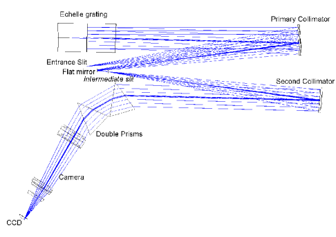
Figure 3: The optical layout of WES with collimators, echelle grating, fold mirror, cross-disperser, and camera.

Figure 4: a)The layout of WES with the mechanics. b) A photograph of WES mounted on the optical bench for initial testing.

2.3.1 Collimators

Two collimators of WES were cut from a single parabolic mirror with a focal length of 925 mm. The main collimator with a size of 230$\times$180 mm transforms the f/10 beam to a collimated beam with a diameter of 92.5 mm. The beams which are dispersed by echelle grating, are again collected by the main collimator and focused at an intermediate focal plane. A flat mirror is placed in front of the intermediate focal plane in order to fold the light path, which reduces the volume of WES and allows an intermediate slit to be placed at the intermediate focal plane. Only the light from the intermediate focal plane can pass the intermediate slit, stopping most of the stray light produced at the echelle grating and roughness of the optical surfaces and edges (Kaufer et al. 1999). The second collimator, also called transfer collimator, with a size of 230$\times$135 mm, transforms the converged beam to a collimated beam cross-dispersed by prisms. A Hartmann diaphragm with left and right semicircle is placed in the collimated beam, in front of the echelle grating, for automatic focusing.

2.3.2 Dispersing element

Because of our compromise between cost and throughput of small telescope, the WES uses a R3 echelle grating with blaze angle of $\theta=71.5^{\circ}$ as the main dispersing element. The echelle grating was made by Newport company with 31.6 grooves/mm and size of 128$\times$254 mm. The surface was aluminum-coated with the peak efficiency of 73% at $\sim$630 nm. The echelle grating is mounted facing downwards to avoid dust settling on the optical surface. The grating is used in quasi-Littrow condition with a slight tilted angle ($0.7^{\circ}$).

The white-pupil layout minimizes the size of the cross-disperser. The WES uses a pair of two identical LF5 prisms with a base length of 103 mm, a width of 125 mm, a height of 134 mm, and an apex angle of 41^∘.

2.3.3 Camera and CCD

The f/3.0 dioptric camera with a diameter of 116mm images the echellogram onto a 2K$\times$2K Andor iKon-L DZ936N-BV CCD with a 13.5 $\mu$m/pixel scale. The image quality of the camera designed for WES is that calculated 80% encircled energy spot diameter is smaller than 25 $\mu$m. The spot diagrams across the echellogram for the complete optical system of WES design is shown in Fig. 5. The free spectral range of WES with 100 spectral orders from 370 nm to 976 nm simulated on the a 2048 $\times$ 2048 13.5 $\mu$m pixels CCD are shown in Fig. 7a. The arrangement of echelle grating and cross disperser results in a line tilt relative to the echelle dispersion direction. Although the geometric effect of line tilt is to degrade the resolving power, this effect is negligible at all but the largest tilts (Hearnshaw et al. 2002). The R3 echelle grating of WES is used in quasi-Littrow condition with a slight tilted angle ($0.7^{\circ}$) causing 4.2^∘ line tilt. Then the whole spectrum is not slightly tilted to align the slit images with the CCD rows specially because the spectral lines tilt little. The impact of slit tilt and anamorphism on spectrograph resolution is negligible as shown in Fig. 6a and Fig. 7b. In order to keep the camera in a very stable mechanically condition for measuring PRV, the symmetrical mountings of camera are manufactured in the shape of circular tube because of its excellent resistance to gravity deformation. The whole barrel of camera is installed on an electric guide rail for automatic focusing. The CCD operates at 0.05MHz with a readout noise of 3.6 e^-. The temperature of the chip is set to -95 ^∘C by water cooling which is good for low dark current and environment stability.

Figure 5: The spot diagrams across the echellogram for the complete optical system of WES design. Wavelength is indicated in $\mu$m above each 1 $\times$ 1 CCD pixels box (13.5 $\mu$m). From bottom left to up right is blue to red. The solid line implies Airy disk.

2.4 Environment Control

The optical elements of WES are all installed on a marble vibration-proof optical bench which is 1500 kilograms with a thickness of 20 cm (see Fig. 4b). There is an air compressor for an air-supported vibration isolation system under the optical bench for avoiding mechanical vibration for frequencies below 3 Hz. Temperature and atmospheric pressure controlled for the long-term are the most important parameters for environment stability. This bench is placed in an air-conditioned room to limit temperature and humidity changes. Unlike the HARPS spectrograph, which is operated in vacuum (Pepe et al. 2000) and the HERMES which was atmospheric pressure controlled (Raskin et al. 2011), WES is just operated in a temperature controlled environment at present (see Fig. 3). The design of atmospheric pressure control for WES will be developed in the near future.

The optical bench is wrapped by a laminated box made of two panels of polyurethane. There is a circulatory pipe with constant temperature water and heat reflecting plate made of aluminum between two panels. The CCD was also wrapped by a polyurethane box to isolate thermal fluctuations. There are two refrigerated and heating circulators outside the air-conditioned room, one for the spectrograph box setting temperature to 20 ^∘C and the other for CCD cooling setting temperature to 18 ^∘C. When using water cooling, the internal fan of the CCD is switched off via the software. The sensors for temperature, humidity, and pressure measurements are placed inside and outside the temperature control box. All of the mounts for the large optical elements (camera, collimators, echelle grating, cross prisms, etc) are made of Invar with very small coefficient of thermal expansion (CTE), 1.6$\times$${10}^{-6}$/^∘C. The mountings of camera lens are manufactured from different cast iron with different CTE, which matches the CTE of the lens. The symmetry of the structure minimizes gravity deformation. All the elements are locked and shut off power after adjustment.

3 Observations and data reduction

We have two observation modes: the normal mode and the PRV mode. In the normal mode, we observe the object at the required spectral resolutions (40,000-55,000) without iodine cell, providing data for common stellar physics research. In the PRV mode, we obtain the spectrum at the spectral resolution of R$\sim$50,000 with iodine cell. We observe a template iodine-free stellar spectrum at higher resolution (R$\sim$55,000). We always arrange the template observations with high quality at very clear nights. Then we also observe a rapidly rotating B star with the iodine cell in order to calculate the instrumental profile at the same night. The template observations can also provide data for studies of stellar abundance, gravity gradient, and other physical parameters, which is crucial for the formation and evolution of planetary systems. We use the same method of RV analysis as described by Sato et al. (2002).

We chose some RV standard stars ($\epsilon$ Vir, $\iota$ Per, $\tau$ Cet, etc) for regular observations to test the stability of the spectrograph and detect the instrumental system drifts. We also observe some targets of known exoplanet hosts ($\beta$ Gem, $\upsilon$ And, etc) for further monitoring to derive accurate parameters of planetary systems and reveal additional planets. We have obtained 106 frames in 25 nights distributed during more than 4 years for $\beta$ Gem (Hatzes et al. 2006). More than 90 objects for RV measurement with V magnitude from 0 to 6 have been observed since 2010 after WES installed.

The raw data reduction is made using standard procedures in the echelle package in Image Reduction and Analysis Facility (IRAF). The reduction procedure is summarized as follows:

• Combination of bias and bias subtraction for the frames of objects, flat fields, ThAr.

• Combining and mosaicing flat fields. Because of the different throughput in the blue and red part of the spectrograph, we acquire flat fields with three different exposure times and combine them respectively. We trim different regions of three different types of flat fields, and then mosaic into one flat field.

• Normalizing the flat field and flat fielding the data.

• Background subtraction. Unlike the long-slit spectrograph, both the sky and the target’s light are recorded at the same location on the CCD with the fiber-fed spectrograph. We should observe the sky spectra separately. The level of scattered light is very low with the layout of white pupil. We can do or skip this step according to our scientific purposes.

• Extraction of the spectra and wavelength calibration.

• Continuum normalization. In the observations with iodine cell, it is difficult to fit the continuum because of iodine absorption spectra superimposed on the stellar spectra. We normalize the stellar spectra divided by the spectra of combined flat field.

4 Performances

4.1 Wavelength range and Spectral resolution

For a fiber-fed spectrograph without FRD effect, the nominal spectral resolution $R=\lambda/\Delta\lambda$ of WES with a collimated beam size of 92.5 mm, a sky aperture of 2.6 arcsec, and a R3 echelle grating at the 1.0 m WHOT is about 44 000. Each image of fiber core is sampled by 3.0 $\times$ 3.0 pixels on the CCD. The resolution can be increased to 57000 with a minimum of 2.2 pixels sampling by narrowing the adjustable slit at the fiber-exit.

The image of the ThAr frame with full slit width is shown in Fig. 6a. We measured the full width at half maximum (FWHM) of the image of fiber core all through the CCD to examine the overall image quality of WES. The FWHMs of all single emission lines are chosen and their contour is shown in Fig. 6b. The image quality at the focal plane is good and uniform, in the sense that the actual average FWHM of the image of fiber core is 3.38 pixels, and the variation is less than 0.86 pixels. We note that the left region has a slightly larger FWHM than the right, which is possibly caused by the measurement accuracy effected by low SNR or a misalignment of the CCD camera with respect to the optical axis. We will consider it in the future adjustment.

The arc spectra allows us to get a dispersion solution (wavelength versus pixel and order number) of WES. We identify the emission lines using the task of “ecidentify” in the echelle package of IRAF with four-order Chebyshev function after tracing and extracting a ThAr frame. The RMS of the identification is 0.003 Å (according to $\sim$0.06 pixels, $\sim$147 m/s). The wavelength range covered by each order and the corresponding sampling ratio per pixel can be derived after the identification (see Fig. 8a). The spectral resolution is defined as $R=\lambda/\Delta\lambda$. We derived the $\Delta\lambda$ from the FWHM of the ThAr emission lines projected alone spectral direction after flux integral along cross-dispersion direction.

The full-frame raw data obtained from $\tau$ Cet shows the position of the curved echellogram on the CCD in Fig. 7b. The rectangular 2K$\times$2K CCD with 13.5$\mu$m per pixel can image 100 orders of continuous spectrum from 371 to 976 nm and 7 further extended orders of slightly truncated spectrum from 976 to 1,100 nm. The spectral resolution power R=$\lambda/\Delta\lambda$ is 40,600 with full slit-width at 550 nm. The maximum spectral resolution is 57,000 with a 2.2 pixels sampling at 550 nm (see Fig. 8b). We set the throughput of full slit-width as 1.0. The spectral resolution and relative throughput of different slit-widths measured through ThAr frames are shown in Table 2. Because we can not measure the slit-width directly, the values of slit-width in Table 2 is converted by the software according to the step of the drive motor and it is the relative value (Coefficient $\times$ Physical width $+$ Constant), not the physical value. So we mainly focus on the resolution and the relative throughput.

Figure 6: a) The full-frame raw data of ThAr. At bottom left the inset shows a magnified section of the echelle image. b) The contour of FWHM measured from the ThAr frame.

Figure 7: a) The free spectral range of WES with 100 orders simulated on the 27.648 $\times$ 27.648 mm CCD, blue is towards the bottom left and red is towards the top right. b) The full-frame raw data of $\tau$ Cet displaying 107 echelle orders of curved echellogram ranging from 3710 to 10998 Å. At bottom left the inset shows a magnified section of the echelle image.

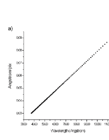
Figure 8: a) The spectral sampling per pixel of each order according to different wavelengths. b) The spectral resolution with 2.2 pixels sampling.

Table 2: The measured spectral resolution and throughput of different slit-widths.

Slit-widtha	Relative throughput	FWHM	Spectral Resolution
($\mu$m)		(pixels)	(R)
135	1.00	3.09	40600
130	0.98	3.01	41700
125	0.96	3.00	41800
120	0.93	2.93	42900
115	0.91	2.90	43300
110	0.87	2.83	44500
105	0.83	2.75	45700
100	0.77	2.69	46700
95	0.74	2.55	49200
90	0.67	2.49	50400
85	0.60	2.38	52900
80	0.53	2.29	54900

Note: ^aThe values is the relative value (Coefficient $\times$ Physical width $+$ Constant), not the physical value.

The IPs of WES with different resolutions, at the center of the 108^th blaze order ($\sim$5560 $\AA$) along the wavelength (CCD line), was modelled through the B-star + I₂ spectrum (Butler et al. 1996; Endl et al. 2000, Sato et al. 2002) as shown in Fig. 9. We modelled the IP with a combination of a central and ten satellite Gaussian profiles which are placed at appropriate intervals and have suitable widths. The IP of WES is symmetric and close to the Gaussian profile nearly, which is very important for the PRV measurement (Kambe et al. 2002).

Figure 9: The IPs of WES with different resolutions, at the center of the 108^th blaze order ( $\sim$5560 $\AA$) along the wavelength (CCD line), derived from B-star + I₂ spectra. The solid and dashed line are the IP from multi and single Gaussian fitting respectively in this data modeling technique.

The cross-disperser provides a minimum order separation of 11 pixels in the reddest part of the spectrum, and a maximum order separation of 26 pixels in the bluest part of the spectrum. Because of more than 3 pixels of FWHM in each order and the possible spectra overlapping redward of 6,000 Å, it is not good enough to use simultaneous thorium technique (Baranne et al. 1996).

Fig. 10 shows the spectra of some blaze orders of $\iota$ Per (HD19733, Spectral Type: F9.5V, Vmag=4.05) observed with 30 min exposure time at R=50,000. The spectra is reduced after continuum normalization.

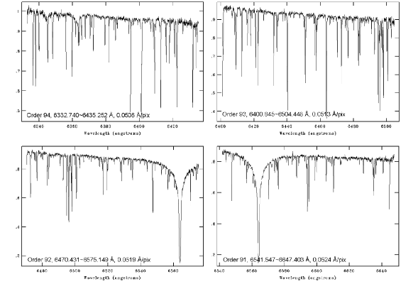
Figure 10: Some blaze orders of the normalized spectra of $\iota$ Per (Vmag=4.05), obtained with 30 min exposure time at R = 50,000.

4.2 Efficiency

The system efficiency is the ratio of photons incident at the top of the atmosphere at zenith and the detected photons on the spectrograph CCD (Aceituno et al. 2013). This efficiency includes atmospheric transparency, throughput of all optical elements, and guiding losses.

We estimated the efficiency of the whole spectroscopic system using as much as possible the specifications given by the corresponding instrument data sheets and the reflectivity or transmissivity of each element we measured. Before the efficiency test, we measured the reflectivity or transmissivity of each element using a spectrophotometer CM-2300d (Konica Minolta, Japan), after we cleaned the optical elements. The efficiency of each element is listed in Table 3. The mean atmospheric transmission is 0.74 in the V band tested by photometric system of WHOT (Hu et al. 2014). The efficiency of 1-m telescope is 0.67, degraded by the main telescope mirror reflections roughly 0.91, the secondary telescope mirror reflections 0.84 and 0.87 pass secondary mirror block. The reflectance of the pick-off mirror is 0.80. The throughput of 0.1 mm guiding pinhole is 0.80 at the median seeing of 1.7^′′, as described in Sect. 2.1. The throughput of 50 $\mu$m fiber optics is 0.58 tested by NIAOT. The efficiency of the spectrograph itself was originally estimated to be around 0.30 in the V band, using the specifications given by data sheets (Table 3). So the overall expected efficiency is 0.74*0.67*0.8*0.8*0.58*0.30=0.055 in the V band, including atmospheric transparency and guiding pinhole losses. The efficiency will be higher at 620nm in the R band.

Table 3: The efficiency of each element

Element	Type	Efficiency	origin
Atmospheric transmission	Transmission	0.74	Measured
Telescope
Main mirror	Mirror reflectivity	0.91	Measured
Secondary mirror	Mirror reflectivity	0.84	Measured
	Secondary mirror block pass	0.87	Data sheet
Pick-off mirror	Mirror reflectivity	0.80	Measured
Pinhole mirror	Throughput at the seeing of 1.7′′	0.80	Calculated
Fiber optics	Throughput of fiber optics	0.58	Measured
Spectrograph
Two collimators	Mirror reflectivity	0.945	Data sheet
Fold mirror	Mirror reflectivity	0.986	Data sheet
Prism
	Total transmission	0.88	Data sheet
	Total entrance/exit transmission	0.916	Data sheet
Echelle grating
	Overfilling	0.89	Data sheet
	Absolute efficiency at 630nm	0.73	Data sheet
Camera	All lenses total transmission	0.81	Data sheet
CCD
	Quantum efficiency	0.89	Data sheet
	Entrance/Exit transmission	0.93	Data sheet

The throughput of the photometric system in each band at WHOT has been estimated by observing a series of standard stars on photometric nights. We arranged efficiency comparison tests between WES and photometric system through dome-flat at the same night. The brightness of the flat field lamp is stable which eliminate the effect of weather and seeing. The specific steps of dome-flat test are as follows:

• In the night without the Moon, the dome was closed completely after dark.

• Open the flat-field lamp half an hour, waiting for the light becomes stable. Make sure that the telescope is not moving.

• Acquire the dome-flat field through the photometric system. In order to avoid shutter effect, the exposure time should not be too short.

• Acquire the dome-flat field through the WES

• Data analysis, specific as follows:

  • Calculate the photon number per square centimeter per second (cm^-2s^-1) obtained from a filter of the photometric system ($N_{phot}$). And extract the spectra of dome-flat obtained from WES.

  • The dome-flat spectrum of WES is convolved with the transmittance curve of the filter. Then the photon number in this band is obtained from WES, ($N_{spec}$), translated to per square centimeter per second according to the area of the pinhole aperture.

  • Through the efficiency of the photometric system, ($E_{phot}$), we can get the efficiency of WES, $E_{spec}=E_{phot}\times(N_{spec}/N_{phot})$.

The dome-flat test shows that the efficiency of WES is 38.5% of photometric system with efficiency 0.183 in V band including atmospheric transparency in October 2010. So the efficiency of WES is 0.385*0.183$\approx$0.070 in the V band without guiding losses. Considering throughput of 0.1 mm guiding pinhole for the point source, the final efficiency is 0.07*0.80=0.056 including atmospheric transparency and guiding loss. It is similar to the value estimated using data sheets and the reflectivity of each element as described above.

Table 4 shows the SNR and efficiency computed using some existing scientific observation data. We acquired a spectrum of HD19445 (Vmag=8.06) in an hour exposure with an SNR of 106 at 550 nm, with the resolution of R$\approx$40,000 and a seeing of 1.4^′′ on November 17, 2010.

In the PRV mode, the throughput of I₂ cell is 0.77 at 550nm, 0.86 at 620 nm. The throughput of slit width is $\sim$0.67 at R=50,000. So the efficiency in the PRV mode is 0.77*0.67$\approx$0.52 of that in normal mode without the I₂ cell and slit at 550nm. The SNR of $\upsilon$ And (Vmag=4.09) is 269 with an exposure of 600 second. Through this observation of $\upsilon$ And, the SNR is estimated to be 112 for Vmag=6 star in 10-min exposure time. The absolute spectral flux (photons cm^-2s^-1Å^-1) of standard stars can be found on the website (http://deep-red.sr.unh.edu/starflux/). We calculated the efficiency of two observation modes using observations of HR982 and $\upsilon$ And at different wavelengths as shown in Fig. 11.

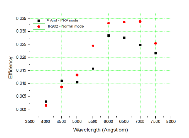
Figure 11: Overall WES efficiency derived from the absolute flux of standard star HR982 and $\upsilon$ And, respectively corresponding to the normal mode and the PRV mode.

Table 4: Some observations of WES.

Object	Exptime	I2 cell	R	Vmag	SNR550nm	Efficiency	Rmag	SNR620nm	Efficiency
	(s)	(Yes/No)				at 550nm			at 620nm
Vega	15	No	50000	0.03	280	0.016	0.07	313	0.032
Deneb	60	No	40000	1.25	383	0.022	1.14	415	0.037
HIP677	60	No	40000	2.06	304	0.029	2.09	322	0.054
HIP96516	1200	No	40000	5.70	228	0.024	5.56	307	0.059
HD19445	3600	No	40000	8.06	106	0.017	7.60	130	0.032
HD115515	1800	No	40000	9.45	48	0.021	9.79	55	0.060
HD71369	360	Yes	50000	3.42	227	0.010	2.76	310	0.016
$\upsilon$ And	600	Yes	50000	4.09	269	0.015	3.64	360	0.028
$\tau$ Cet	600	Yes	50000	3.50	307	0.011	2.88	472	0.023

The best efficiency that already appeared is 2.9% at 550nm, which is lower than expected. Because of no cleaning of the optical instruments for a long time, suboptimal seeing, imperfect weather and telescope guiding for observation, the efficiency cannot reach expected value.

4.3 Stray light

The stray light is primarily reduced by the intermediate slit in front of the flat mirror, as described in Sect 2.3.1. The distribution of stray light is very local, and became relevant when the signal is weak at the blue part of focal plane. We determine the stray light level scattered into a pixel, by the ratio of spectral intensity in the inter-order to the peak flux in the adjacent orders with the frames of flat-field. The highest stray light level is 5.3% at blue part of the focal plane, and less than 0.7% at most of red focal plane.

4.4 Stability and RV precision

During the commissioning periods without the most stable conditions, the temperature in the spectrograph box changed 1.7 ^∘C in six months from September 2010 to February 2011, causing 7.3-pixel shift in cross-dispersion direction and 0.8-pixel shift in dispersion direction on the CCD. The spectrograph is thermally stabilised to $\pm$0.03 ^∘C in one day, $\pm$0.04 ^∘C in one week after the commissioning.

The RV method for exoplanet research requires very high precision. For example, Jupiter imparts a velocity of 12.47 m/s on the Sun. If we want to determine a Doppler shift of 10 m/s at the optical band, the wavelength shift at 5,000 Å is about 0.00016 $\AA$ which correspond to 0.004 pixels on the CCD of WES. So RV observations have high demands on spectrograph stability.

The radial velocities of $\epsilon$ Vir (HD 113226, Vmag=2.79, G8III) calculated from the observations of WES are shown in Fig. 12 in order to test measurement precision of radial velocity. The standard deviation (as “std” shown in the figure) of the measured radial velocities is 9.15 m/s over a 6-month period (183 days), with the internal measurement error (as “std/sqrt(n)” shown in the figure) of 2.64 m/s. As shown in bottom panel of Fig. 12, the standard deviation is 14.04 m/s over a 54-month period (1,617 day, 4.4 years), with the internal measurement error of 1.93 m/s.

We also analyzed the radial velocities of $\iota$ Per (HD 19373, Vmag=4.05, F9.5V) as shown in Fig. 13. The standard deviation of the RVs is 10.43m/s over a 10-month period (302 days), with the internal measurement error of 3.14 m/s (top panel of Fig. 13). The standard deviation of the RVs is 14.63m/s over a 35-month period (1,068 days), with the internal measurement error of 2.28 m/s (bottom panel of Fig. 13).

The measurement errors of RV obtained from each frame are about 2 - 10 m/s in most of time, but larger (40 - 60 m/s) in JD (-2450000) from 6024 to 6026 in Fig. 12, due to the instability of I₂ temperature. The unstability was caused by the problem of conducting wire which affected the accuracy of the instrument profile measurement.

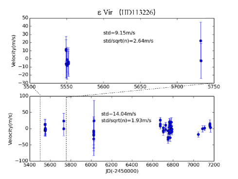
Figure 12: The radial velocities of $\epsilon$ Vir (HD113226) obtained from WES.

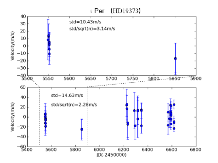
Figure 13: The radial velocities of $\iota$ Per (HD19373) obtained from WES.

Wittenmyer et al. (2015) analyzed 38 observations of $\beta$ Gem (HD 62509, Vmag=1.14, K0III) over a 500-day baseline, with a mean internal velocity uncertainty of 8.6 m/s. All published velocities spanning more than 25 years are included to fit a Keplerian orbit to the planetary signal. The RMS about the fit to the velocities obtained from WES is only 7.3 m/s, better than any previous published data set, demonstrating that the data acquisition and RV extraction techniques of WES are robust.

4.5 Results about fiber-shaking device

The SNR will be deduced by modal noise which leads to a non-uniform distribution of light at the fiber exit. A fiber-shaking device allowing non-harmonic movement of the fiber will changes the speckle distribution quickly on the fiber exit during exposure time (Sect2.2). The light path of flat-field and ThAr lamp on the fiber-head is stable. The modal distribution will not be changed when the fiber-shaking device is off. The difference of SNR between the fiber shaking device on and off is showen in Fig. 14. The measured average SNR of flat-field frame is about 310 and 200 at 7000 - 8000 $\AA$ when the fiber-shaking device is on and off respectively (top panel of Fig. 14). The measured SNRs almost reach the predicted ones calculated from pure photon statistics using the square root of mean photon numbers ($\sqrt{N}$), expected for a well exposed flat-field spectrum when the fiber-shaking device is on. The fiber shaking device improves the scrambling of flat field frames and ThAr frames. The increase of SNR can optimize flat fielding and wavelength calibration in data preprocessing.

The light from star at fiber-head changed the input light path at high-frequency because of atmospheric perturbation in most seeing situations, as the effect of a fiber-shaking device. The modal distribution also changed quickly when the fiber-shaking device is off. We did the fiber-shaking device test with observations for spectral type B stars (see the bottom panel of Fig. 14). The SNR did not change significantly when the fiber-shaking device is on and off, and it also reached the highest SNR expected with seeing 2^′′. During exposure of short time and very good seeing, the SNR may increase or remain unchanged when the fiber-shaking device is on, which still need further tests.

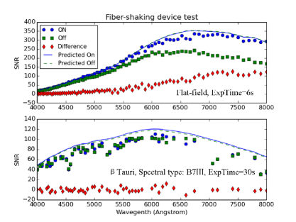
Figure 14: Measured and predicted SNR when the fiber-shaking device on and off. Top panel: SNR difference of Flat-field; Bottom panel: SNR difference of B star.

5 Summary and future prospects

Table 5: Main characteristics of WES.

Telescope interface module
Guiding CCD	SBIG ST2000 XMI, field of view: $\sim 6^{\prime}\times 6^{\prime}$
Pinhole aperture	0.1 mm (2.6′′)
Fiber optics
Fiber core	50 $\mu$m
Entrance focal ratio	f/3.67
Exit focal ratio	$\sim$f/3.7
Spectrograph	white-pupil layout
Collimated beam diameter	92.5 mm
Collimator focal ratio	f/10
Echelle grating	Newport R3 (71.5∘), 31.6 grooves/mm, 128 $\times$ 254 mm
Cross-disperser	2 LF5 prisms, 41∘ apex angle,
	103 (base) $\times$ 125 (width) $\times$ 134 (height) mm
Dioptric camera
Camera focal ratio	f/3.0
Camera aperture	116 mm diameter
Detector	Andor iKon-L DZ936N-BV, 2K$\times$ 2K 13.5-$\mu$m pixels
Total size of spectrograph	2.3 (L) $\times$ 1.85 (W) $\times$ 1.5 (H) m
Wavelength range
	371-976 nm (in continuous 100 orders)
	976-1,100 nm (in extended 7 orders)
Resolving power	at 550nm
Spectral resolution per pixel	0.044 Å/pix
$R=\lambda/\Delta\lambda$ with slit	40,600-57,000
Separation between orders	11-26 pixels from red to blue
Temperature stabilitiy
Temperature change in one day	$\pm$0.03 ∘C
Temperature change in one week	$\pm$0.04 ∘C
Limiting magnitudes	at 550nm
The normal mode	Vmag=8 for SNR=100 in 1-hour exposure
The PRV mode	Vmag=6 for SNR=110 in 10-min exposure
Stabilitiy for the PRV mode	The standard deviation of RV standard star
Short-period	$\sim$10 m/s in 10 months
Long-period	$<$15 m/s in 54 months (4.4 years)

After commissioning since October 2010, WES has reached the predicted performance. The main characteristics of WES are given in Table 5. In the normal mode, with a seeing of 1.4^′′, the limiting magnitude obtained for 1 hour exposure that produces an SNR of more than 100 at 550 nm with the resolution of 40,000 was around Vmag=8. In the PRV mode, with the resolution of 50,000 and iodine cell, the SNR will reach more than 110 at 550 nm for Vmag=6 in 10-min exposure.

The temperature change is 0.04^∘C in one week, much lower than expected (0.5^∘C), which is good for PRV observations. The limiting factors of RV accuracy seem to be: (1) insufficient SNR; (2) unstable optical depth of the I₂ cell due to unstable temperature control; (3) systematic error in the instrument profile (IP), etc. So we will focus on the stability of optical element, environment control, and guiding telescope carefully in future observations.

Using the RV standard stars ($\epsilon$ Vir, $\iota$ Per) and an exoplanet hosting star ($\beta$ Gem), we estimated that RV precision is about 10 m/s in short period of time (10 months), showing that WES can be used to detect and research giant exoplanets (Cao et al. 2014). The standard deviation of RV is better than 15 m/s and the internal measurement error is lower than 3 m/s over 4.4 years time. The RV precision will be better after optimizing the code for measurement in the near future. The WES with RV observing system has joined the East Asia exoplanet searching network (EAPSNET) and the Pan-Pacific Planet Search (PPPS), collaborating with exoplanet hunters from China, Japan, Korea and Australia (Izumiura. 2005; Liu et al. 2009; Sato et al. 2008; Wittenmyer et al. 2011), to search for the new worlds around giant and dwarf stars.

Appendix A: ZEMAX optical description

Table A1 summarises the ZEMAX data of all optical surfaces of the WES. The optical system has been optimised by considering the measured values of the radii of curvature of the elements.

Table A1: ZEMAX optical surface data.

Surf	Type	Radius	Thickness	Glass	Diameter	Conic	Comment
OBJ	STANDARD	Infinity	0		0	0	Source
1	COORDBRKa	-	925		-	-	Tilt Inbeam
STO	STANDARDb	-1850	-925	MIRROR	339.9809	-1	Collimator-1
3	COORDBRKc	-	0		-	-	Littrow twist 1/2
4	COORDBRKd	-	0		-	-	Blaze tilt
5	COORDBRK	-	0		-	-	90deg tilt of Grating
6	DGRATINGe	Infinity	0	MIRROR	393.7426	0	Echelle Grating
7	COORDBRK	-	0		-	-	90deg backtilt of Grating
8	COORDBRK	-	0		-	-	Blaze backtilt
9	COORDBRK	-	0		-	-	Lttrow twist 2/2
10	COORDBRK	-	925		-	-	Shift back littrow
11	STANDARDb	-1850	-879	MIRROR	297.2057	-1	Collimator-1
12	STANDARD	Infinity	46	MIRROR	51.84238	0	Fold Mirror
13	STANDARD	Infinity	925		58.22472	0	Intermediate Slit
14	COORDBRK	-	0		-	-
15	STANDARDf	-1850	-852	MIRROR	389.1993	-1	Collimator-2
16	COORDBRKg	-	0		-	-	Center coord
17	COORDBRKh	-	0		-	-	Prism-1
18	STANDARD	Infinity	-65	LF5	119.2219	0	Prism-1 front
19	COORDBRKi	-	0		-	-	Prism-1
20	STANDARDj	Infinity	0		156.3835	0	Prism-1 back
21	COORDBRKh	-	-79.25		-	-	Prism-1
22	COORDBRKh,k	-	0		-	-	Prism-2
23	STANDARD	Infinity	-65	LF5	122.2081	0	Prism-2 front
24	COORDBRKi	-	0		-	-	Prism-2
25	STANDARDh,j	Infinity	0		146.435	0	Prism-2 back
26	COORDBRK	-	-60		-	-	Prism-2
27	STANDARD	Infinity	-5		116	0
28	STANDARD	Infinity	0		116	0	Circular buffle
29	STANDARD	-185.13	-23.5	S-FPL53	120	-0.3635	Lens 1 front
30	STANDARD	267.9	-15.16		120	0	Lens 1 back
31	STANDARD	231.7	-10	H-K9L	120	0	Lens 2 front
32	STANDARD	-173.868	-15	S-FPL53	120	0	Lens 2 back/Lens 3 front
33	STANDARD	2228.84	-231.95		120	0	Lens 3 back
34	STANDARD	-100	-32	H-QK3L	100	0	Lens 4 front
35	STANDARD	301.04	-30.67		100	0	Lens 4 back
36	STANDARD	130.3006	-8	H-F4	76	0	Lens 5 front
37	STANDARD	Infinity	-54.94		76	0	Lens 5 back
38	STANDARD	Infinity	0		33.59009	0
39	COORDBRK	-	0		-	-
40	STANDARD	Infinity	-2.3	LITHOSIL-Q	40	0	Dewar front
41	STANDARD	Infinity	-9	VACUUM	40	0	Dewar back
IMA	STANDARD	Infinity		VACUUM	25.65352	0	CCD

Notes: ^aTilt About X: 7.64; ^bY- Decenter: 113.8; ^cTilt About X: 0.7; ^dTilt About Y: 71.5; ^eX- Decenter: 123.76; ^fY- Decenter: -145.6; ^gDecenter Y: -124; Tilt About X: 1.4; ^hTilt About X: -33.8; ⁱTilt About X: 41; ^jY- Decenter: 24.256232; ^kDecenter Y: 20.6;

References

- (1) Aceituno, J., Sánchez, S. F, Grupp, F., Lillo, J., et al. 2013, A&A 552, A31
- (2) Baranne, A. 1988, in Very Large Telescopes and their Instrumentation, ed. M.-H. Ulrich (European Southern Observatory), 1195
- (3) Baranne, A., Queloz, D., Mayor, M., et al. 1996, A&AS, 119, 373
- (4) Butler, R. P., Marcy, G. W., Williams, E., et al. 1996, PASP, 108, 500
- (5) Endl, M., Kürster, M., & Els, S. 2000, A&A, 362, 585.
- (6) Cao, C., Ren, D., Gao, D., et al. 2014, in IAU Symp. 293, Formation, Detection, and Characterization of Extrasolar Habitable Planets, ed. N. Haghighipour & J.-L. Zhou (Cambridge: Cambridge Univ. Press), 33
- (7) Grupp, F. 2003, A&A, 412, 897
- (8) Guo, D.-F., Hu, S.-M., Chen, X., Gao, D.-Y., & Du, J.-J. 2014, PASP, 126, 496
- (9) Harrison, G. R., Loewen, E. G., & Wiley R. S. 1976, APPLIED OPTICS, 15, 971
- (10) Hatzes, A. P., Cochran, W. D., Endl, M., et al. 2006, A&A, 457, 335
- (11) Hearnshaw, J. B., Barnes, G. M., Kershaw, G. M, et al. 2002, Experimental Astronomy, 13, 59
- (12) Hu, S.-M., Han, S.-H., Guo, D.-F., & Du, J.-J. 2014, RAA, 14, 719
- (13) Izumiura, H. 2005, Korean Astronomical Society, 38, 81
- (14) Kambe, E., Sato, B., Takeda, Y., Ando, H., Noguchi, K., Aoki, W., Izumiura, H., Wada, S., et al. 2002, PASJ, 54, 865
- (15) Kaufer, A., & Pasquini, L. 1998, Proc. SPIE, 3355, 844
- (16) Kaufer, A., Stahl, O., Tubbesing, S., et al. 1999, The Messenger, vol. 95, p. 8-12
- (17) Liu, Y.-J., Sato, B., Zhao, G., Ando, Hiroyasu 2009, ReA&A, 9, 1.
- (18) Mayor, M., & Queloz, D. 1995, Nature, 378, 355
- (19) Marcy, G. W., & Butler, R. P. 1992, PASP, 104, 270
- (20) Pfeiffer, M. J., Frank, C., Baumueller, D., Fuhrmann, K., & Gehren, T. 1998, A&AS, 130, 381
- (21) Pepe, F., Mayor, M., Delabre, B., et al. 2000, in “Optical and IR Telescope Instrumentation and Detectors”, SPIE 4008, 582
- (22) Queloz, D., & Mayor, M. 2001, Messenger, 105, 1
- (23) Ramsey 1988, in Fiber optics in astronomy, ed. Samuel C. Barden (San Francisco: A.S.P. Conference Series), 3, 26
- (24) Raskin, G., van Winckel, H., Hensberge, H., et al. 2011, A&A, 526, A69.
- (25) Sato, B., Kambe, E., Takeda, Y., & Izumiura, H. 2002, PASJ, 54, 873
- (26) Sato, B., Izumiura, H., Toyota, E., et al. 2008, PASJ, 60, 539
- (27) Sato, B., Kambe, E., Takeda, et al., 2005a, PASJ, 57, 97
- (28) Valenti, J. A., Butler, R. P. & Marcy, G. W. 1995, PASP, 107, 966.
- (29) Wittenmyer, R. A., Gao, D., Hu, S. M., et al. 2015, PASP, 127, 1021
- (30) Wittenmyer, R. A., Endl, M., Wang, L., et al. 2011b, ApJ, 743, 184
- (31)