Generalized Entropy Concentration for Counts

Abstract

The phenomenon of entropy concentration provides strong support for the maximum entropy method, MaxEnt, for inferring a probability vector from information in the form of constraints. Here we extend this phenomenon, in a discrete setting, to non-negative integral vectors not necessarily summing to 1. We show that linear constraints that simply bound the allowable sums suffice for concentration to occur even in this setting. This requires a new, ‘generalized’ entropy measure in which the sum of the vector plays a role. We measure the concentration in terms of deviation from the maximum generalized entropy value, or in terms of the distance from the maximum generalized entropy vector. We provide non-asymptotic bounds on the concentration in terms of various parameters, including a tolerance on the constraints which ensures that they are always satisfied by an integral vector. Generalized entropy maximization is not only compatible with ordinary MaxEnt, but can also be considered an extension of it, as it allows us to address problems that cannot be formulated as MaxEnt problems.

Keywords: maximum generalized entropy, counts, concentration, linear constraints, inequalities, norms, tolerances

1 Introduction

The maximum entropy method or principle, originally proposed by E.T. Jaynes in 1957, now appears in standard textbooks on engineering probability and information theory, [PP02], [CT06]. Commonly referred to as MaxEnt, the principle essentially states that if the only information available about a probability vector is in the form of linear constraints on its elements, then, among all others, the preferred probability vector is the one that maximizes the Shannon entropy under these constraints. Besides the great wealth and diversity of its applications, MaxEnt can be justified on a variety of theoretical grounds: axiomatic formulations ([SJ80], [Ski89], [Csi91], [Cat12]), the concentration phenomenon ([Jay83], [Gr8], [Cat12], [OG16]), decision- and game-theoretic interpretations ([Gr8] and references therein), and its unification with Bayesian inference ([GC07], [Cat12]).

Among these justifications, in a discrete setting, the appeal of concentration lies in its conceptual simplicity. It is essentially a combinatorial argument, first presented by E.T. Jaynes [Jay83], who called it “concentration of distributions at entropy maxima”. The concentration viewpoint was further developed in [Gr8] and [OG16], which presented generalizations, improved results, eliminated the asymptotics, and studied additional aspects.

In this paper we adopt a discrete, finite, non-probabilistic, combinatorial approach, and show that the concentration phenomenon arises in a new setting, that of non-negative vectors which are not necessarily density vectors. Among other things, this requires introducing a new, ‘generalized’ entropy measure. This new concentration phenomenon lends support to an extension of the MaxEnt method to what we call “maximum generalized entropy”, or MaxGEnt.

The basics of entropy concentration are easiest to explain in terms of the abstract “balls and bins” paradigm ([Jay03]). There are $m$ labelled, distinguishable bins, to which $n$ indistinguishable balls are to be allocated one-by-one. The final content of the bins is described by a count vector $\nu=(\nu_{1},\ldots,\nu_{m})$ which sums to $n$, and a corresponding frequency vector $f=\nu/n$, summing to 1. Suppose that the frequency vector must satisfy a set of linear equalities and inequalities, $\sum_{i}a_{ij}f_{i}=b_{j}$ and $\sum_{i}a_{ij}f_{i}\leqslant b_{j}$, with $a_{ij},b_{j}\in\mathbb{R}$. The concentration phenomenon is that as $n$ becomes large, the overwhelming majority of the allocations which accord with the constraints have frequency vectors that are close to the $m$-vector which maximizes the Shannon entropy subject to the constraints.

In our extension there is no longer a given number of balls. Therefore we cannot define a unique frequeny vector, but must deal directly with count vectors $\nu$ whose sums are unknown (Example 1.1 below makes this clear). The linear constraints are now placed on the counts $\nu_{i}$, again with coefficients in $\mathbb{R}$. Our only assumption about the constraints is that they limit the sums of the count vectors to lie in a finite range $[s_{1},s_{2}]$. With just this assumption, we show that as the counts are allowed to become larger and larger (by a process of scaling the problem, explained in §3), the vast majority of allocations that satisfy the constraints in fact have count vectors close to the non-negative $m$-vector $x^{\ast}$ that maximizes the generalized entropy $G(x)$. A precise statement of this concentration phenomenon needs some additional preliminaries, and is given at the end of this section.

Our main results are, in §2, a new generalized entropy function $G$, defined on arbitrary non-negative vectors, which reduces to the Shannon entropy $H$ on vectors summing to 1; its properties are studied in §2 and §3, where the scaling process is also introduced. In §4 we demonstrate the new concentration pheonomenon with respect to deviations from the maximum generalized entropy value $G^{\ast}$. Theorem 4.1 gives a lower bound on the ratio of the number of realizations of the MaxGEnt vector to that of the set of count vectors $\nu$ whose generalized entropies $G(\nu)$ are far from the maximum value $G^{\ast}$. Then Theorem 4.2 completes the picture by deriving how large the problem must be for the above ratio to be suitably large. In §5 we establish concentration with respect to the $\ell_{1}$ norm distance of the count vectors from the MaxGEnt vector; we present Theorems 5.1 and 5.2, which are analogous to those of §4, and also Theorem 5.3, an optimized version of Theorem 5.2. In all the theorems, ‘far’, ‘large’, etc. are defined in terms of parameters, introduced in Table 1.2 below. None of our results involve any asymptotic considerations, and we give a number of numerical illustrations.

The following example demonstrates the basic issues referred to above in a very simple setting, which highlights the differences with the usual frequency vector case. After this, we proceed to the precise statement of generalized entropy concentration.

Example 1.1

A number of indistinguishable balls are to be placed one-by-one in three bins, red, green, and blue. The final content $(\nu_{r},\nu_{g},\nu_{b})$ of the bins must satisfy $\nu_{r}+\nu_{g}=4$ and $\nu_{g}+\nu_{b}\leqslant 6$. Thus the total number of balls that may be put in the bins cannot be too small, e.g. 3, or too large, e.g. 20. Each assignment of balls to the bins is described by a sequence made from the letters $r,g,b$, with a corresponding count vector $\nu=(\nu_{r},\nu_{g},\nu_{b})$; the sequence can be of any length $n$ consistent with the constraints. Table 1.1 lists all the count vectors that satisfy the constraints, their sums $n$, and their number of realizations $\#\nu$, i.e. the number of sequences that result in these counts, given by a multinomial coefficient, e.g. $\binom{7}{3,1,3}=140$. [In the terminology of the theory of types, $\#\nu$ is the size of the type class $T(\nu/n)$.] What can be said about the “most likely” final content of the bins?

$\nu_{r}$ $\nu_{g}$ $\nu_{b}$ $n$ $\#\nu$ 0 4 0 4 1 1 3 0 4 2 2 0 6 3 1 0 4 4 0 1 1 0 4 1 5 5 1 3 1 20 2 2 1 30 3 1 1 20 4 0 1 5

$\nu_{r}$ $\nu_{g}$ $\nu_{b}$ $n$ $\#\nu$ 0 4 2 6 15 1 3 2 60 2 2 2 90 3 1 2 60 4 0 2 15 1 3 3 7 140 2 2 3 210 3 1 3 140 4 0 3 35

$\nu_{r}$ $\nu_{g}$ $\nu_{b}$ $n$ $\#\nu$ 2 2 4 8 420 3 1 4 280 4 0 4 70 3 1 5 9 504 4 0 5 126 4 0 6 10 210

Table 1.1: The count vectors $\nu=(\nu_{r},\nu_{g},\nu_{b})$ satisfying $\nu_{r}+\nu_{g}=4,\nu_{g}+\nu_{b}\leqslant 6$, their sum $n$, and their number of realizations $\#\nu$. If we had the additional constraint $\nu_{r}+\nu_{g}+\nu_{b}=7$, only the $n=7$ section of the table would apply, and we would reduce to a MaxEnt problem.

This example makes two points. First, it does not seem possible to find a single frequency vector that can be naturally associated with the problem; without that, one cannot think about maximizing the usual entropy. Second, one may think that starting with the largest possible number of balls, 10 in this case, would lead to the greatest number of realizations. But this is not so: the count vector with the most realizations sums to 9, and even vectors summing to 8 have more realizations than the one summing to 10.

Next we give a precise statement, GC below, of generalized entropy concentration. To do that we need to (a) define the generalized entropy and describe how to find the vector that maximizes it, (b) specify how to derive the bounds $s_{1},s_{2}$ from the constraints, (c) describe how to ensure the existence of integral solutions (count vectors) to the constraints, and (d) introduce parameters that define the concentration.

To find the vector with the largest number of realizations in a problem like that of Example 1.1, we first assume that the problem does not admit arbitrarily large solutions. This is made precise in (1.2) below, but a necessary condition is that each element of $\nu$ appears in some constraint. Next we relax the integrality requirement on the counts, and set up a continuous maximization problem

$$\begin{array}[]{c}\max_{x\in\mathcal{C}}G(x),\text{\quad where}\quad G(x)=-\sum_{i}x_{i}\ln x_{i}+\left(\sum_{i}x_{i}\right)\ln\left(\sum_{i}x_{i}\right)\\ \text{and}\qquad\mathcal{C}=\{x\in\mathbb{R}^{m}\mid A^{E}x=b^{E},A^{I}x\leqslant b^{I},x\geqslant 0\}.\end{array},$$ (1.1)

Here $G(x)$ is the generalized entropy of the real vector $x\geqslant 0$, and the constraints on $x$ are expressed via the real matrices $A^{E},A^{I}$ and vectors $b^{E},b^{I}$. We assume that the constraints (a) are satisfiable, and (b) they bound the possible sums of the $x\in\mathcal{C}$; this is equivalent to assuming that all $x_{i}$ are bounded. Thus $\mathcal{C}$ is a non-empty polytope in $\mathbb{R}^{m}$ and (1.1) is a concave maximization problem (see e.g. [BV04]) with a solution $x^{\ast}$. We will refer to (1.1) as the “MaxGEnt problem” and to $x^{\ast}$ as “the MaxGEnt vector” or as “the optimal relaxed count vector”. Since the function $G$ is concave but not strictly concave, see Fig. 2.1 in §2, it is not immediate that the solution $x^{\ast}$ is unique; however, we show that this is the case in §2.4.

The boundedness assumption is that $\sum_{i}x_{i}$ lies between (finite) numbers $s_{1}$ and $s_{2}$; these are determined by solving the linear programs

$$s_{1}\;\triangleq\min_{x\in\mathcal{C}}(x_{1}+\cdots+x_{m}),\qquad s_{2}\;\triangleq\max_{x\in\mathcal{C}}(x_{1}+\cdots+x_{m}).$$ (1.2)

(A technicality is that the constraints may force some elements of $x^{\ast}$ to be 0; for reasons explained in §3 it is convenient to eliminate such elements, so that in the end all elements of $x^{\ast}$ can be assumed to be positive reals.) Finally, from $x^{\ast}$ we derive an integral vector $\nu^{\ast}$, to which we refer as the optimal, or MaxGEnt count vector, by a procedure explained in §3.

Because in the end we are interested only in integral/count vectors in the set $\mathcal{C}$ of (1.1), we will introduce, as explained in §3, tolerances on the satisfaction on the constraints, governed by a parameter $\delta$. This will turn $\mathcal{C}$ into $\mathcal{C}(\delta)$. To describe the concentration we need two more parameters, $\varepsilon$ specifying the strength of the concentration, and $\eta$ or $\vartheta$ describing the size of the region in which it occurs. The parameters are summarized in Table 1.2.

$\delta$:	relative tolerance in satisfying the constraints
$\varepsilon$:	concentration tolerance, on number of realizations
$\eta$:	relative tolerance in deviation from the maximum generalized entropy value $G^{\ast}$
$\vartheta$:	absolute tolerance in deviation (distance) from the optimal relaxed count vector $x^{\ast}$

Table 1.2: Parameters for the concentration results.

Lastly, when we have ordinary entropy and frequency vectors, concentration occurs by increasing the number of balls $n$. With count vectors, this is replaced by increasing $b^{E},b^{I}$, the values of the constraints. The increase we consider here consists in multiplying these vectors by a scalar $c>1$, a process which we call scaling. This scaling results in larger and larger count vectors being admissible and is described in detail in §3.

Now we can give the precise statement of the concentration phenomenon for count vectors:

GC: Theorems 4.2 and 5.2 compute a number $\hat{c}(\delta,\varepsilon,\eta)$ and $\hat{c}(\delta,\varepsilon,\vartheta)$, respectively, called the “concentration threshold”, such that if the problem data $b^{E},b^{I}$ is scaled by any factor $c\geqslant\hat{c}$, the number of assignments/sequences that result in the optimal count vector $\nu^{\ast}$ is at least $1/\varepsilon$ times greater than the number of all assignments that result in count vectors with entropy less than $(1-\eta)G^{\ast}$ or farther than $\vartheta$ from $x^{\ast}$ by $\ell_{1}$ norm.

Significance

In a problem where the only available information is embodied in the constraints and which otherwise admits a large number of probability vectors as solutions, the concentration phenomenon provides a powerful argument for the MaxEnt method, which selects a particular solution, the one with maximum entropy, in preference to all others. Likewise, the concentration results in this paper support the maximization of generalized entropy for problems involving general non-negative vectors. We believe that MaxGEnt can be considered to be a compatible extension of MaxEnt. The compatibility is that any MaxEnt problem over the reals with constraints $A^{E}x=b^{E},A^{I}x\leqslant b^{I}$ can be formulated as a MaxGEnt problem of the form (1.1) with the same constraints, plus the constraint $\sum_{i}x_{i}=1$; both problems will have the same solution $x^{\ast}\in\mathbb{R}^{m}$, and the maximum entropy $H(x^{\ast})$ will equal the maximum generalized entropy $G(x^{\ast})$. Also, if the constraints of the MaxGEnt problem either explicitly or implicitly fix the value of $\sum_{i}x_{i}$, then the problem can be reduced to a MaxEnt problem over the reals. The extension consists in the fact that MaxGEnt addresses problems involving un-normalized vectors that cannot be formulated as MaxEnt problems, as we saw in Example 1.1; more examples of such problems are given in §3, §4, and §5.

Related work

Our term “generalized entropy” for $G$ is neither imaginative nor distinctive, and there are many other generalized entropy measures. The most general of these are Csiszár’s $f$-entropies and $f$-divergences [Csi96], and the related $\Phi$-entropies of [BLM13]. Any relationship of $G$ to $\Phi$-entropies remains to be investigated. The function $G$, in the form of the log of a multinomial coefficient with “variable numerator”, appeared in [OS06] and [Oik12].

The problem of inferring a non-negative real vector from information in the form of linear equalities was considered by Skilling [Ski89], where such vectors were termed “positive additive distributions”, and by Csizsár, [Csi91], [Csi96]. Both authors gave axiomatic justifications, which do not involve probabilities, for minimizing the I-divergence, a generalization of relative entropy to un-normalized vectors. A further generalization is the $\alpha,\beta$ divergences of [CCA11]. We discuss a connection between I-divergence and our generalized entropy in §2.5.

With respect to concentration, recent developments for the discrete, normalized case were given in [OG16]. The continuous normalized case, for relative entropy, is examined in [Cat12] from the viewpoint of information geometry. Countable spaces are also treated in [Gr8]. But these references do not provide explicit bounds such as the ones here and in [OG16]. To our knowledge, concentration for non-density vectors has not been studied before.

The structure and some of the presentation of this paper are similar to [OG16] because of the similar subject matter, entropy concentration from a combinatorial viewpoint. Many of the results here that appear similar to those of section III of [OG16] are generalizations of those results, insofar as $G$ is a generalization of $H$. However the main theorems here do not actually subsume corresponding theorems in [OG16], because in both cases the theorems include optimizations specific to count or frequency vectors, respectively.

2 The generalized entropy $G$

In this section we introduce the generalized entropy function $G$, and study its properties, relationships with other functions, and its maximization under linear constraints.

Given a real vector $x\geqslant 0$, its generalized entropy is

$$G(x)\;\triangleq\;H(x)+\Bigl{(}\sum_{i}x_{i}\Bigr{)}\ln\Bigl{(}\sum_{i}x_{i}\Bigr{)}\;=\;\Bigl{(}\sum_{i}x_{i}\Bigr{)}H(\chi),\quad x\geqslant 0.$$ (2.1)

Here $H(x)$ is the form $-\sum_{i}x_{i}\ln x_{i}$ extended to vectors in $\mathbb{R}_{+}^{m}$ that are not necessarily density vectors, and $\chi$ is the density, or normalized, or probability, vector corresponding to $x$. (2.1) gives two ways to look at $G(x)$: it is the (extended) entropy of $x$ plus the sum of $x$ times its log, or the sum of $x$ times the ordinary entropy of the normalized $x$. If $x$ is already normalized $G(x)$ coincides with $H(x)$. Fig. 2.1 is a plot of $G(x)$ for $m=2$.

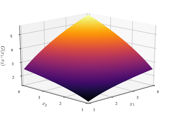
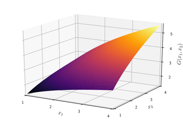
Figure 2.1: $G(x_{1},x_{2})$. Note that $G(x,x)=(2\ln 2)x$, which destroys the strict concavity of $G$.

2.1 Basic properties

We list some important properties of the function $G$:

P1

$G(x_{1},\ldots,x_{m})$ is the log of the multinomial coefficient $\binom{x_{1}+\cdots+x_{m}}{x_{1},\ldots,x_{m}}$ to “second Stirling order”: by using the first two terms of $\ln x!\;=\;x\ln x-x+\frac{1}{2}\ln x+\ln\sqrt{2\pi}+\frac{\vartheta}{12x},\vartheta\in(0,1),$we find that

$$\ln\binom{x_{1}+\cdots+x_{m}}{x_{1},\ldots,x_{m}}\approx G(x_{1},\ldots,x_{m}).$$

This interpretation was given in [Oik12], where it was used to derive “most likely” matrices, i.e. those with the largest number of realizations, from incomplete information.

P2

$G$ is related to the ordinary entropy (of density vectors) and the extended entropy (of arbitrary non-negative vectors) $H$ in the two ways specified in (2.1).

P3

Unlike the entropy of normalized vectors which is bounded by $\ln m$, the generalized entropy $G(x)$ increases without bound as the elements of $x$ become larger: for any $x,y$, if $y\geqslant x$ then $G(y)\geqslant G(x)$. This is shown in Proposition 2.3. One consequence is that if $x,y$ are close in norm, i.e. $\|x-y\|\leqslant\zeta$, $|G(x)-G(y)|$ cannot be bounded by an expression involving only $m$ and $\zeta$.

P4

$G(x)$ is positive, unless $x$ has just one non-0 element, in which case $G(x)=0$. This follows from the second form in (2.1).

P5

Given any p.d. $p=(p_{1},\ldots,p_{m})$ and any $n$-sequence $\sigma$ with count vector $\nu$, the probability of $\sigma$ under $p$ can be written as

$${\Pr}_{p}(\sigma)=e^{-(G(\nu)+nD(f\|p))}$$

where $D(\cdot\mid\cdot)$ is the divergence, or relative entropy, between two probability vectors and $f=\nu/n$ is the frequency vector corresponding to $\nu$. By substituting $G(\nu)=nH(f)$ we obtain the well-known expression for the same probability in terms of the ordinary entropy of a frequency vector.

P6

Like the ordinary or the extended $H,$ $G(x_{1},\ldots,x_{m})$ is concave over the domain $x_{1}>0,\ldots,x_{m}>0$, but unlike $H$, it is not strictly concave. See Proposition 2.2 in §2.2.

P7

The maximum of $G(x_{1},\ldots,x_{m})$ subject just to the constraint $\sum_{i}x_{i}=s$ is $s\ln m$. When $s=1$, $x$ is a density vector and this reduces to the maximum of $H$.

P8

What is the relationship between maximizing $G$ and maximizing the extended $H$? Consider maximizing the first form in (2.1), subject to $A^{E}x=b^{E},A^{I}x\leqslant b^{I}$, by imposing the additional constraint $\sum_{i}x_{i}=s$ and treating $s$ as a parameter taking values in $[s_{1},s_{2}]$. For a given $s$, there will be a unique maximum since $H$ is strictly concave. Further, some $s=s^{\ast}$ will achieve $\max_{s}\max_{x}(s\ln s+H(x))$ subject to $A^{E}x=b^{E},A^{I}x\leqslant b^{I},\sum_{i}x_{i}=s$; this maximum value will equal $G(x^{\ast})$. Using the second form in (2.1) we see that there is a similar relationship between maximizing $G(x)$ and maximizing the function $sH(x/s)$.

P9

$G$ has a scaling (or homogeneity) property, which $H$ does not: for any $c>0$ and any $x\in\mathbb{R}_{+}^{m}$, $G(cx)=cG(x)$. This is most easily seen from the second form in (2.1).

P10

$G$ has a further important scaling property: if $x^{\ast}$ maximizes $G(x)$ under $Ax\leqslant b$, then for any $c>0$, $cx^{\ast}$ maximizes $G(x)$ under $Ax\leqslant cb$. We show this in §3.3, Proposition 3.2.

2.2 Monotonicity and concavity properties

As we noted in property P3 in §2.1, $G$ is an increasing function in the sense that

Proposition 2.1

For any $x,y$, if $y\geqslant x$ then $G(y)\geqslant G(x)$, and if the inequality is strict in some places, then $G(y)>G(x)$.

We will use this property in §2.3. Now we turn to concavity.

The extended ordinary entropy $H$ is strictly concave, and in addition, strongly concave for any modulus $\gamma\leqslant 1/a$ when defined over $[0,a]^{m}$. The generalized entropy $G$ is also concave, but neither strictly concave, nor strongly concave for any modulus. However $-G$ is sublinear, whereas $-H$ is not. These properties are collected in the following proposition:

Proposition 2.2

1. The function $G(x_{1},..,x_{m})$ is concave over $\mathbb{R}_{+}^{m}$.

2. G is not strictly concave over $\mathbb{R}_{+}^{m}$.

3. $G$ is not strongly concave over $\mathbb{R}_{+}^{m}$ for any modulus $\gamma>0$.

4. If the definition of $G$ is extended over all of $\mathbb{R}^{m}$ by setting $G(x)=-\infty$ if any $x_{i}$ is $<\;0$, then for all $\alpha,\beta>0$ and for all $x,y\in\mathbb{R}^{m}$, $G(\alpha x+\beta y)\;\geqslant\;\alpha G(x)+\beta G(y)$.

The last property is stronger than (implies) concavity since $\alpha,\beta$ are not required to sum to 1. The absence of strict concavity means that more care is needed with maximization, we address this in §2.4.

2.3 Lower bounds

Given a point $x$, if some other point $y$ is close to it in the distance/norm sense, how much smaller than $G(x)$ can $G(y)$ be? We will need the answer in §4. Proposition 2.1 implies that if we have a hypercube centered at $x$, say $\|x-y\|_{\infty}\leqslant\zeta$, then $G(\cdot)$ attains its maximum at the “upper right-hand” corner of the hypercube and its minimum at the “lower left-hand” corner. Specifically, for any $\zeta>0$, let $\boldsymbol{\zeta}$ denote the $m$-vector $(\zeta,\ldots,\zeta)$, and let $x\geqslant\boldsymbol{\zeta}$. Then it can be seen from Proposition 2.1 that for any $y\geqslant 0$

$$\|x-y\|_{\infty}\leqslant\zeta\quad\Rightarrow\quad G(x-\boldsymbol{\zeta})\leqslant G(y)\leqslant G(x+\boldsymbol{\zeta}).$$ (2.2)

Using this observation we can show that

Lemma 2.1

Given $\zeta>0$ and $x,y\in\mathbb{R}^{m}_{+}$, if $x>\boldsymbol{\zeta}$ and $\|y-x\|_{\infty}\leqslant\zeta$, then

$$G(y)\;\geqslant\;G(x)-\Bigl{(}\sum_{i}\ln\frac{\|x\|_{1}}{x_{i}}\Bigr{)}\zeta-\frac{1}{2}\Bigl{(}\sum_{i}\frac{1}{x_{i}-\zeta}-\frac{m}{\|x\|_{1}/m-\zeta}\Bigr{)}\zeta^{2}.$$

The coefficient of $\zeta^{2}$ is positive unless all $x_{i}$ are equal, in which case it becomes 0.

The lower bound above does not depend on $y$, only on $x$ and $\zeta$. The restriction $x>\boldsymbol{\zeta}$ applies to the ‘reference’ point $x$, not to the ‘variable’ $y$; see also Remark 4.2. Lastly, since $\|x-y\|_{1}\leqslant\zeta\Rightarrow\|x-y\|_{\infty}\leqslant\zeta$, the lemma holds also when the $\ell_{\infty}$ norm is replaced by the $\ell_{1}$ norm.

We will use Lemma 2.1 in §4.1 to bound how far from the maximum $G(x^{\ast})$ the value $G(x)$ can be if $x$ is close to $x^{\ast}$. We also comment there, Remark 4.3, on how the above bound compares to bounds obtainable from the relationship between (ordinary) entropy difference and $\ell_{1}$ norm.

2.4 Maximization

Let $\mathcal{C}(0)$ denote the subset of $\mathbb{R}^{m}$ defined by the constraints in (1.1). Here we point out that despite the fact that $G$ is not a strictly concave function (recall Proposition 2.2, part 2), the point $x^{\ast}$ solving (1.1) is the unique optimal solution of our maximization problem, and occupies a special location in $\mathcal{C}(0)$:

Proposition 2.3

1. The point $x^{\ast}$ is the unique optimal solution of problem (1.1).

2. The set $\mathcal{C}(0)$ does not contain any $x$ s.t. $x\geqslant x^{\ast}$ with at least one strict inequality.

Figure 2.2 illustrates the first statement of the proposition.

Figure 2.2: A 2-dimensional polytope $\mathcal{C}(0)$. By Proposition 2.3, $x^{\ast}$ can lie only on the heavy black line.

Finally we look at the form of the solution $x^{\ast}$ in terms of Lagrange multipliers. The Lagrangean for problem (1.1) is

$$L(x,\lambda^{E},\lambda^{I})=G(x)-\lambda^{E}\cdot(A^{E}x-b^{E})-\lambda^{I}\cdot(A^{I}x-b^{I}),$$ (2.3)

where $\lambda^{E},\lambda^{I}$ are the vectors of the Lagrange multipliers corresponding to the equality and inequality constraints. The solution $x^{\ast}$ will satisfy some of the inequality constraints with equality (and these are called binding or active at $x^{\ast}$), and some with strict inequality. It is known that multipliers $\lambda^{I}_{j}$ corresponding to inequalities non-binding at $x^{\ast}$ will be 0, while the rest of them will be $\geqslant\;0$ (see, e.g., [HUL96], Ch. VII, §2.4). Thus, denoting the sub-vector of $\lambda^{I}$ corresponding to binding inequalities by $\lambda^{\operatorname{BI}}$ and the corresponding sub-matrix of $A^{I}$ by $A^{\operatorname{BI}}$, it follows from (2.3) that $x^{\ast}$ can be written as

$$x^{\ast}_{j}=(x^{\ast}_{1}+\cdots+x^{\ast}_{m})e^{-(\lambda^{E}\cdot A^{E}_{.j}+\lambda^{\operatorname{BI}}\cdot A^{\operatorname{BI}}_{.j})}.$$ (2.4)

This expression determines the elements of the density vector $\chi^{\ast}=x^{\ast}/\sum_{i}x^{\ast}_{i}$ in terms of the multipliers, but it does not determine the vector $x^{\ast}$ itself.

Remark 2.1

It is clear that the form (2.4) cannot express any elements of $x^{\ast}$ that are 0, if the multipliers $\lambda$ are to be finite. To avoid introducing special cases in the sequel to handle the zeros, we will assume as a convenience that any elements of the solution to problem (1.1) that are forced to be exactly 0 by the constraints are eliminated from consideration either before or after the solution is found. We have already alluded to this after (1.2). Thus, whenever we speak of $x^{\ast}$ in what follows we will assume that all of its elements are positive. See Example 5.3 in §5. A more detailed discussion of the issue of 0s is in [OG16], §II.A.

Example 2.1

Returning to Example 1.1, it is possible to maximize $G$ analytically under the given constraints. Introducing real variables $x_{1},x_{2},x_{3}$ corresponding to $\nu_{r},\nu_{g},\nu_{b}$ and letting the constraints be $x_{1}+x_{2}=a$ and $x_{2}+x_{3}\leqslant b$, the solution turns out to be

$$x^{\ast}_{1}=s^{\ast}-b,\quad x^{\ast}_{2}=a+b-s^{\ast},\quad x^{\ast}_{3}=s^{\ast}-a,\qquad s^{\ast}=\frac{a+b+\sqrt{a^{2}+b^{2}}}{2}.$$

Further, the bounds $s_{1},s_{2}$ of  (1.2) on the possible sums are $s_{1}=a$ and $s_{2}=a+b$. We see that the MaxGEnt solution to the problem is never trivial, in the sense that for all $a,b$, we have $s_{1}<s^{\ast}<s_{2}$; when $a=b$ we have $s^{\ast}=\frac{1}{2}\left(1+\frac{\sqrt{13}}{5}\right)s_{2}\approx 0.861s_{2}$. With $a=4,b=6$ we find $s^{\ast}=8.61$ and $x^{\ast}=(2.61,1.39,4.61)$; compare with Table 1.1.

2.5 A connection with I-divergence

For density vectors, the relationship between ordinary entropy $H(x)$ and divergence $D(x\|y)$ is well known: with uniform $y$, $D(x\|y)$ reduces to $H(x)$ to within a constant, and its minimization is equivalent to the maximization of $H(x)$. Here we look at whether $G(x)$ has any analogous properties.

First, if in $D(x\|y)$ we take $y$ to have all of its elements equal to $\sum_{i}x_{i}$, we obtain $-G(x)$. However, this is merely a formal relationship. For example, minimizing $D(x\|y)$ with respect to $x$ when $y=\left(\sum_{i}x_{i},\ldots,\sum_{i}x_{i}\right)$ cannot be given the same interpretation as minimizing $D(x\|y)$ with respect to $x$ given a fixed ‘prior’ $y$. So even if $x,y$ summed to 1, neither the axiomatic nor the concentration justifications for cross-entropy minimization would apply.

Second, the concentration properties we establish in §4 and §5 support the maximization of $G(x)$ as a method of inference of non-negative vectors from limited information. Another method for doing this, suggested in [Ski89], [Csi96], is based on minimizing the I-divergence (information divergence) between non-negative vectors

$$\mathcal{D}(u\|v)\;\triangleq\;\sum_{i}u_{i}\ln\frac{u_{i}}{v_{i}}-\sum_{i}u_{i}+\sum_{i}v_{i},\qquad u,v\in\mathbb{R}^{m}_{+}.$$ (2.5)

This reduces to $D(u\|v)$ when $u,v$ sum to 1. The inference problem is “problem (iii)” in [Csi96]: infer a non-negative function $p(z)$, not necessarily summing or integrating to 1, given that (a) it belongs to a certain feasible set $\mathcal{F}$ of functions defined by linear equality constraints, and (b) a default model $q(z)$. It is shown that the solution of this problem is the $p^{\ast}\in\mathcal{F}$ that minimizes the I-divergence $\mathcal{D}(p\|q)$. (Recently, minimization of I-divergence and generalizations to “$\alpha,\beta$ divergences” has found many applications in the area known as “non-negative matrix factorization”, see [CCA11].)

There is a relationship between minimizing I-divergence and maximizing generalized entropy:

Proposition 2.4

Let $(A^{E},b^{E}),(A^{I},b^{I})$ be linear equality and inequality constraints on a vector in $\mathbb{R}_{+}^{m}$, and let $x^{\ast}$ be the solution of the MaxGEnt problem with these constraints on $x$. Given a prior $v\in\mathbb{R}^{m}_{+}$, let $u^{\ast}(v)$ be the solution to the minimum I-divergence problem with the same constraints on $u$. Then there is a prior $\tilde{v}$ which makes the two solutions coincide, i.e. $u^{\ast}(\tilde{v})=x^{\ast}$. That prior is $\tilde{v}=(s^{\ast},\ldots,s^{\ast})$.

This follows from the fact that the minimum I-divergence solution to a problem with prior $v$ and constraints $A^{E}u=b^{E}$ and $A^{I}u\leqslant b^{I}$ on $u$ is

$$u^{\ast}_{j}=v_{j}e^{-(\lambda^{E}\cdot A^{E}_{.j}+\lambda^{\operatorname{BI}}\cdot A^{\operatorname{BI}}_{.j})}.$$ (2.6)

If we set $v_{j}=s^{\ast}$, it can be seen from expression (2.4) that $u^{\ast}_{j}=x^{\ast}_{j}$ satisfies (2.6).

Inference by minimizing I-divergence under equality constraints has an axiomatic basis, but as pointed out in §3 and §7 of [Csi96], the combinatorial, concentration rationale that we are advocating here does not seem to apply to it. Proposition 2.4 shows that the adoption of a particular prior furnishes this rationale, except that this prior cannot be properly viewed as independent of the solution (posterior) $u^{\ast}$. This dependence may shed some light on the difficulty of finding the concentration rationale in general. [As an illustration, Example 2.1 can be solved by I-divergence minimization assuming a constant prior $v=(\alpha,\alpha,\alpha)$. An analytical solution $u^{\ast}$ is possible, and it has the same form as the MaxGEnt solution, but it is a function of $\alpha\in(0,\infty)$; the question then becomes what value to adopt for $\alpha$.]

3 Constraints, scaling, sensitivity, and the optimal count vector

In §3.1 we discuss the necessity of introducing tolerances into the constraints defining the MaxGEnt problem, and in §3.2 the effect of these tolerances on the maximization of $G$. In §3.3 we turn to the scaling of the problem, i.e. multiplying the data vector $b$ by some $c>0$, and the important properties of this scaling. Lastly, in §3.4 we discuss the optimal, or MaxGEnt count vector $\nu^{\ast}$, constructed from the real vector $x^{\ast}$ solving problem (1.1).

3.1 Constraints with tolerances

We pointed out the necessity of introducing tolerances into linear constraints when establishing concentration of ordinary entropy in [OG16]. The constraints involved real coefficients, and the solutions had to be rational (frequency) vectors with a particular denominator. Here the solutions need to be integral (count) vectors, but the equality constraints may not have any integral solution; e.g. $x_{1}-x_{2}=1,x_{1}+x_{2}=4$ are satisfied only for $(x_{1},x_{2})=(2.5,1.5)$, and likewise with inequalities, e.g. $1.3\leqslant x_{1}\leqslant 1.99$. We therefore define the set of real $m$-vectors $x$ that satisfy the constraints in (1.1) with a relative accuracy or tolerance $\delta\geqslant 0$:

$$\mathcal{C}(\delta)\triangleq\{x\in\mathbb{R}^{m}:b^{E}-\delta|\beta^{E}|\leqslant A^{E}x\leqslant b^{E}+\delta|\beta^{E}|,A^{I}x\leqslant b^{I}+\delta|\beta^{I}|\},$$ (3.1)

where $\beta^{E},\beta^{I}$ are identical to $b^{E},b^{I}$, except that any elements that are 0 are replaced by appropriate small positive constants. The tolerances are only on the values $b$ of the constraints, not on their structure $A$. Recall that the generalized entropy is maximized over $\mathcal{C}(0)$, which we have assumed to be non-empty, problem (1.1).

There are three main points concerning the introduction of $\delta$. First, the existence of integral solutions, which is elaborated in Proposition 3.1 below. Second, and related to the first, $\delta$ ensures that the concentration statement GC in §1 holds for all scalings of the problem larger than a threshold $\hat{c}$. This is analogous to having concentration for frequency (rational) vectors hold for all denominators $n$ larger than some $N$, as in [OG16]. Third, $\delta$ has an effect on the maximization of $G$; this the subject of §3.2.

Proposition 3.1 below gives the fundamental facts about the existence of count vectors in $\mathcal{C}(\delta)$. Given an $x$ in $\mathcal{C}(0)$, any other vector $y$ close enough to it is in $\mathcal{C}(\delta)$, and, if $\delta$ is not too small, the count vector obtained by rounding $x$ element-wise is in $\mathcal{C}(\delta)$; in other words, for every real vector in $\mathcal{C}(0)$ there is an integral vector in $\mathcal{C}(\delta)$. The “close enough” and the “not too small” depend on a number $\vartheta_{\infty}$:

Proposition 3.1

With $\beta^{E},\beta^{I}$ as in (3.1), define

$$\vartheta_{\infty}\;\triangleq\;\min(|\beta^{E}|_{\min}/\interleave A^{E}\interleave_{\infty},|\beta^{I}|_{\min}/\interleave A^{I}\interleave_{\infty}),$$

or $\infty$ if there are no constraints. Then if $x$ is any point in $\mathcal{C}(0)$,

1. Given any $\delta>0$, any $y\in\mathbb{R}_{+}^{m}$ such that $\|y-x\|_{\infty}\;\leqslant\delta\;\vartheta_{\infty}$ is in $\mathcal{C}(\delta)$.

2. In particular, if $\delta\geqslant 1/(2\vartheta_{\infty})$, the integral/count vector $[x]$ is in $\mathcal{C}(\delta)$.

As we add constraints to a problem, $\vartheta_{\infty}$ can only decrease, or at best stay the same. This proposition is used in §4.3, eq. (4.23), and in §5.2, after (5.9).

Example 3.1

Fig. 3.1 shows a network consisting of 6 nodes and 6 links. The links are subject to a certain impairment $x$ and $x_{i}$ is the quantity associated with link $i$. The impairment is additive, e.g. its value over the path $AB$ consisting of links $4,1,6$ is $x_{4}+x_{1}+x_{6}$.

Figure 3.1: Data $b$ on the impairment $x$ in a 6-node, 6-link network.

Suppose that $x$ is measured over the 3 paths $AB,BC,CA$, and it is also known that the access links 4, 5, 6 contribute no more than a certain amount, as shown in Fig. 3.1. The structure matrices $A^{E},A^{I}$ and data vectors $b^{E},b^{I}$ then are

$$\small A^{E}=\left[\begin{array}[]{cccccc}1&0&0&1&0&1\\ 0&0&1&0&1&1\\ 0&1&0&1&1&0\end{array}\right],\quad b^{E}=\left[\begin{array}[]{c}b_{1}\\ b_{2}\\ b_{3}\end{array}\right],\quad A^{I}=\left[\begin{array}[]{cccccc}0&0&0&1&0&0\\ 0&0&0&0&1&0\\ 0&0&0&0&0&1\end{array}\right],\quad b^{I}=\left[\begin{array}[]{c}b_{4}\\ b_{4}\\ b_{4}\end{array}\right].$$

The problem is to infer the impairment vector $x$ from the measurement vector $b$. Clearly, the values of the $b_{i}$ depend on the chosen units and can change under various conditions, whereas the elements of $A^{E},A^{I}$ are constants defining the structure of the network, and independent of any units.

Suppose we take $(b_{1},\ldots,b_{4})=(10.5,18.3,8.7,4)$. Then with $\beta^{E},\beta^{I}=b^{E},b^{I}$ we have in Proposition 3.1 $|b^{E}|_{\min}/\interleave A^{E}\interleave_{\infty}=8.7/3$ and $|b^{I}|_{\min}/\interleave A^{I}\interleave_{\infty}=4/1$, so $\vartheta_{\infty}=2.9$. The vector $x=(6.591,5.326,13.26,1.120,2.253,2.789)$ satisfies the constraints exactly. The rounded vector $[x]=(7,5,13,1,2,3)$ is in the set $\mathcal{C}(\delta)$ defined by (3.1) for any $\delta\geqslant 0.172$.

3.2 Effect of tolerances on the optimality of $x^{\ast}$

With the constraints $x_{1}-x_{2}=1,x_{1}+x_{2}=4,$and $x_{1},x_{2}\geqslant 0$, $\mathcal{C}(0)$ is a 0-dimensional polytope in $\mathbb{R}^{2}$, the point $(2.5,1.5)$. However, introducing the tolerance  $\delta=0.05$ turns the equalities into inequalities and $\mathcal{C}(0.05)=\{0.95\leqslant x_{1}-x_{2}\leqslant 1.05,3.8\leqslant x_{1}+x_{2}\leqslant 4.2\}$ becomes 2-dimensional. Apart from the change in dimension, $\mathcal{C}(0.05)$ also contains the point $(2.55,1.55)$ at which $G$ assumes a value greater than $G^{\ast}=G(2.5,1.5)$, its maximum over $\mathcal{C}(0)$. This must be taken into account, since concentration refers to the vectors in $\mathcal{C}(\delta)$, not those in $\mathcal{C}(0)$. The following lemma shows that the amount by which the value of $G$ can exceed $G^{\ast}$ due to the widening of the domain $\mathcal{C}(0)$ to $\mathcal{C}(\delta)$ is bounded by a linear function of $\delta$; it generalizes Prop. II.2 of [OG16] for the ordinary entropy $H$:

Lemma 3.1

Let $(\lambda^{E},\lambda^{\operatorname{BI}})$ be the vector of Lagrange multipliers in (2.4) corresponding to the solution $G^{\ast}=G^{\ast}(0),x^{\ast}=x^{\ast}(0)$ of the maximization problem (2.1). Define

$$\Lambda^{\ast}\;\triangleq\;|\lambda^{E}|\cdot|\beta^{E}|+\lambda^{\operatorname{BI}}\cdot|\beta^{\operatorname{BI}}|,\qquad\Lambda^{\ast}\geqslant G^{\ast}.$$

Then with $\delta\geqslant 0$, for any $\nu\in\mathcal{C}(\delta)$

$$G(\nu)\;\leqslant\;G^{\ast}+\Lambda^{\ast}\delta-nD(f\|\chi^{\ast}),$$

where $n=\sum_{i}\nu_{i}$, $f$ is the frequency vector corresponding to $\nu$, and $\chi^{\ast}$ is the density vector corresponding to $x^{\ast}$.

The upper bound on $G(\nu)$ is at least $(1+\delta)G^{\ast}-nD(f\|\chi^{\ast})$. When $\delta=0$ the lemma says simply that $G^{\ast}$ is the maximum of $G$ over $\mathcal{C}(0)$. The $D(\cdot\|\cdot)$ term is positive, and equals 0 iff $\nu=\alpha x^{\ast}$ for some $\alpha>0$. Leaving aside that this is possible only for special $x^{\ast}$ and $\alpha$, Lemma 3.1 says that if the resulting $\nu$ is in $\mathcal{C}(\delta)$, then $G(\nu)=\alpha G^{\ast}\leqslant G^{\ast}+\Lambda^{\ast}\delta$, i.e. the allowable $\alpha$ is limited by $\delta$. Also, if we have even one equality constraint, $\delta$ limits the size of the allowable $\alpha$ even further.

3.3 Scaling of the data and bounds on the allowable sums

We establish a fundamental property, P10 in §2.1, of maximizing the generalized entropy $G$: if the problem data $b$ is scaled by the factor $c>0$, all aspects of the solution scale by the same factor.

Proposition 3.2

Suppose that the relaxed count vector $x^{\ast}$ maximizes $G(x)$ under the linear constraints $A^{E}x=b^{E},A^{I}x\leqslant b^{I}$, which also imply that $\sum_{i}x_{i}$ is between the bounds $s_{1},s_{2}$. Let $c>0$ be any constant. Then the vector $cx^{\ast}$ maximizes $G(x)$ under the scaled constraints $A^{E}x=cb^{E},A^{I}x\leqslant cb^{I}$, the maximum value of $G$ is $cG(x^{\ast})$, and the new bounds on $\sum_{i}x_{i}$ are $cs_{1},cs_{2}$.

How do $s_{1}$ and $s_{2}$, defined in (1.2), depend on the structure matrices $A^{E},A^{I}$ and the data $b^{E},b^{I}$? In general, the problem of bounding $s_{1}$ or $s_{2}$ doesn’t have a simple answer: by scaling the variables, any linear program whose objective function is a positive linear combination of the variables can be converted to one where the objective function is simply the sum of the variables. But in some special cases we can derive simple bounds on $s_{1}$ and $s_{2}$:

Proposition 3.3

Bounds on the sums $s_{1}$ and $s_{2}$.

1. If there are some equality constraints, then $s_{1}\geqslant\|b^{E}\|_{1}/\interleave(A^{E})^{T}\interleave_{\infty}$. (This bound can only increase if there are also inequalities.)

2. Suppose all of $A^{E},A^{I},b^{E},b^{I}$ are $\geqslant 0$, and each $x_{i}$ occurs in at least one constraint. Then $s_{2}\leqslant\sum_{i}b^{E}_{i}/\alpha^{E}_{i}+\sum_{i}b^{I}_{i}/\alpha^{I}_{i}$, where $\alpha^{E}_{i}$, $\alpha^{I}_{i}$, is the smallest non-zero element of row $i$ of $A^{E}$, respectively $A^{I}$, if that element is $<1$, and 1 otherwise.

Recall from §1 that “each $x_{i}$ occurs in at least one constraint” is a necessary condition for the problem to be bounded. The proposition applies to Example 3.1: we find that $s_{1}\geqslant(b_{1}+b_{2}+b_{3})/2$ and $s_{2}\leqslant b_{1}+b_{2}+b_{3}+b_{4}$.

3.4 The optimal count vector $\nu^{\ast}$

Given the relaxed optimal count vector $x^{\ast}$, we construct from it a count vector $\nu^{\ast}$ which is a reasonable approximation to the integral vector that solves problem (1.1), in the sense that (a) its sum is close to that of $x^{\ast}$, and (b) its distance from $x^{\ast}$ is small in $\ell_{1}$ norm. These properties will be needed in §4 and §5. We will require $\nu^{\ast}$ to sum to $n^{\ast}$, where

$$n^{\ast}\triangleq\lceil s^{\ast}\rceil,\quad s^{\ast}\triangleq\sum_{i}x^{\ast}_{i}.$$ (3.2)

For any $x\geqslant 0$, let $[x]$ be the vector obtained by rounding each of the elements of $x$ up or down to the nearest integer. $\nu^{\ast}$ is obtained from $x^{\ast}$ by a process of rounding and adjusting:

Definition 3.1 ([OG16], Defn. III.1)

Given $x^{\ast}$, form the density vector $\chi^{\ast}=x^{\ast}/s^{\ast}$ and set $\tilde{\nu}=[n^{\ast}\chi^{\ast}]$. Construct $\nu^{\ast}$ by adjusting $\tilde{\nu}$ as follows. Let $d=\sum_{i}\tilde{\nu}_{i}-n^{\ast}\in\mathbb{Z}$. If $d=0$, set $\nu^{\ast}=\tilde{\nu}$. Otherwise, if $d<0$, add 1 to $|d|$ elements of $\tilde{\nu}$ that were rounded down, and if $d>0$, subtract 1 from $|d|$ elements that were rounded up. The resulting vector is $\nu^{\ast}$.

We will refer to $\nu^{\ast}$ as “the optimal count vector” or “the MaxGEnt count vector” (even though it is not unique). It sums to $n^{\ast}$, and does not differ too much from $x^{\ast}$ in norm:

Proposition 3.4

The optimal count vector $\nu^{\ast}$ of Definition 3.1 is such that

$$\sum_{1\leqslant i\leqslant m}\nu^{\ast}_{i}=n^{\ast},\quad\|\nu^{\ast}-x^{\ast}\|_{1}\leqslant\frac{3m}{4}+1,\quad\|\nu^{\ast}-x^{\ast}\|_{\infty}\leqslant 1,\quad\|f^{\ast}-\chi^{\ast}\|_{1}\leqslant\frac{3m}{4n^{\ast}}.$$

There are other approximations to the integral solution of problem (1.1); for example, simply $[x^{\ast}]$ achieves smaller norms than $\nu^{\ast}$: $\|[x^{\ast}]-x^{\ast}\|_{1}\leqslant m/2$, $\|[x^{\ast}]-x^{\ast}\|_{\infty}\leqslant 1/2$. ($[x^{\ast}]$ is the point of $\mathbb{N}^{m}$ that minimizes the Euclidean distance $\|\nu-x^{\ast}\|_{2}$ from $x^{\ast}$.) But $[x^{\ast}]$ does not have the required sum $n^{\ast}$.

Another, more sophisticated definition for $\nu^{\ast}$, would use the solution of the integer linear program $\min_{\nu\in\mathbb{N}^{m}}\sum_{i=1}^{m}|\nu_{i}-x^{\ast}_{i}|$ subject to $\sum_{i=1}^{m}\nu_{i}=n^{\ast}$. [This is a linear program because $\min_{z}\sum_{i}|z_{i}-c_{i}|$ is equivalent to $\min_{a,z}\sum_{i}a_{i}$ subject to $a_{i}\geq z_{i}-c_{i},a_{i}\geq-(z_{i}-c_{i})$.] A $\nu^{\ast}$ better than that of Definition 3.1 would improve the bound in (4.9) below.

4 Concentration with respect to entropy difference

It is not clear that concentration should occur at all in a situation like the one of Example 1.1. The fact that $G$ has a global maximum $G^{\ast}$ over $\mathcal{C}(0)$ is not enough. In this section we demonstrate that concentration around $G^{\ast}$ does indeed occur, in the sense of the statement GC of §1, pertaining to entropies $\eta$-far from $G^{\ast}$. This is done in two stages, by Theorem 4.1 in §4.2 and Theorem 4.2 in §4.3.

Consider the count vectors that sum to $n$ and satisfy the constraints. We divide them into two sets, $\mathcal{A}_{n},\mathcal{B}_{n}$, according to the deviation of their generalized entropy from $G^{\ast}$: given $\delta,\eta>0$,

$$\begin{array}[]{lll}\mathcal{A}_{n}(\delta,\eta)&\triangleq&\{\nu\in N_{n}\cap\mathcal{C}(\delta),G(\nu)\geqslant(1-\eta)G^{\ast}\},\\ \mathcal{B}_{n}(\delta,\eta)&\triangleq&\{\nu\in N_{n}\cap\mathcal{C}(\delta),G(\nu)<(1-\eta)G^{\ast}\}.\end{array}$$ (4.1)

Irrespective of the values of $\delta$ and $\eta$, $\mathcal{A}_{n}(\delta,\eta)\uplus\mathcal{B}_{n}(\delta,\eta)=N_{n}\cap\mathcal{C}(\delta)$. Now we discuss the possible range of $n$.

We have assumed that the problem constraints $A^{E}x=b^{E},A^{I}x\leqslant b^{I}$ imply that $s_{1}\leqslant\sum_{i}x_{i}\leqslant s_{2}$, where the bounds $s_{1},s_{2}$ on the sum of $x$ are found by solving the linear programs (1.2). So any integral vector that satisfies the constraints exactly, i.e. is in $\mathcal{C}(0)$, must have a sum $n$ between $n_{1}=\lceil s_{1}\rceil$ and $n_{2}=\lfloor s_{2}\rfloor$. We will use a slight modification of this definition

$$n_{1}\triangleq\lceil s_{1}\rceil,\quad n_{2}\triangleq\lceil s_{2}\rceil.$$ (4.2)

With $n^{\ast}$ defined by (3.2), we have $n_{1}\leqslant n^{\ast}\leqslant n_{2}$. We may assume without loss of generality that $n_{1}\leqslant n_{2}+1$; otherwise all count vectors sum to a known $n$, and we reduce to the case of frequency vectors which was studied in [OG16].

Remark 4.1

There is a certain degree of arbitrariness (or flexibility) in the definitions of $n_{1},n_{2}$. Setting $n_{1}=\lceil s_{1}\rceil,n_{2}=\lfloor s_{2}\rfloor$ says that the allowable sums are those of count vectors which belong to $\mathcal{C}(0)$; it does not say that the only allowable vectors are those in $\mathcal{C}(0)$. Now it could be argued that after introducing the tolerance $\delta$, the numbers $n_{1},n_{2}$ should be allowed to become functions of $\delta$. However, this would introduce significant extra complexity. Our definition makes concessions to simplicity by restricting somewhat the allowable sums, and by slightly adjusting the value of $n_{2}$ to handle the ‘boundary’ case $\lfloor s_{2}\rfloor<s^{\ast}\leqslant s_{2}$ more easily.

Having defined the range of allowable sums $n$ as $n_{1}\leqslant n\leqslant n_{2}$, we will use the (disjoint) unions of the sets (4.1) over $n\in\{n_{1},\ldots,n_{2}\}$

$$\begin{array}[]{lll}\mathcal{A}_{n_{1}:n_{2}}(\delta,\eta)&\triangleq&\left\{\nu\middle|\;\sum_{i}\nu_{i}=n,n_{1}\leqslant n\leqslant n_{2},\nu\in\mathcal{C}(\delta),G(\nu)\geqslant(1-\eta)G^{\ast}\right\},\\ \mathcal{B}_{n_{1}:n_{2}}(\delta,\eta)&\triangleq&\left\{\nu\middle|\;\sum_{i}\nu_{i}=n,n_{1}\leqslant n\leqslant n_{2},\nu\in\mathcal{C}(\delta),G(\nu)<(1-\eta)G^{\ast}\right\}.\end{array}$$ (4.3)

Irrespective of $\delta$ and $\eta$ we have

$$\mathcal{A}_{n_{1}:n_{2}}(\delta,\eta)\;\uplus\;\mathcal{B}_{n_{1}:n_{2}}(\delta,\eta)\;=\;N_{n_{1}:n_{2}}\cap\mathcal{C}(\delta).$$ (4.4)

We note the following relationship among the numbers of realizations of the optimal count vector $\nu^{\ast}$ and those of the sets $\mathcal{A}_{n_{1}:n_{2}}(\delta,\eta)$ and $\mathcal{B}_{n_{1}:n_{2}}(\delta,\eta)$: if $\nu^{\ast}\in\mathcal{A}_{n_{1}:n_{2}}(\delta,\eta)$, then

$$\begin{array}[]{rrrrrrrrr}\displaystyle\frac{\#\nu^{\ast}}{\#\mathcal{B}_{n_{1}:n_{2}}(\delta,\eta)}&\geqslant&\displaystyle\frac{1}{\varepsilon}&\displaystyle\Rightarrow&\displaystyle\frac{\#\mathcal{A}_{n_{1}:n_{2}}(\delta,\eta)+\#\;\mathcal{B}_{n_{1}:n_{2}}(\delta,\eta)}{\#\mathcal{A}_{n_{1}:n_{2}}(\delta,\eta)}&\displaystyle\leqslant&1+\varepsilon&\Rightarrow&\\ &&&&\displaystyle\;\frac{\#\mathcal{A}_{n_{1}:n_{2}}(\delta,\eta)}{\#(N_{n_{1}:n_{2}}\cap\mathcal{C}(\delta))}&\geqslant&\displaystyle\frac{1}{1+\varepsilon}&>&\displaystyle 1-\varepsilon.\end{array}$$ (4.5)

In other words, if the single vector $\nu^{\ast}$ dominates the set $\mathcal{B}_{n_{1}:n_{2}}$ w.r.t. realizations, then the set $\mathcal{A}_{n_{1}:n_{2}}$ dominates the set $N_{n_{1}:n_{2}}\cap\mathcal{C}(\delta)$ likewise.

The concentration statement GC in §1 says that given $\delta,\varepsilon,\eta>0$, there is a number $\hat{c}=\hat{c}(\delta,\varepsilon,\eta)\geqslant 1$ such that when the data $b^{E},b^{I}$ are scaled by any factor $c\geqslant\hat{c}$, then

$$\nu^{\ast}\in\mathcal{A}_{n_{1}:n_{2}}(\delta,\eta)\qquad\text{and}\qquad\frac{\#\nu^{\ast}}{\#\mathcal{B}_{n_{1}:n_{2}}(\delta,\eta)}\;\geqslant\;\frac{1}{\varepsilon}.$$ (4.6)

We establish the inequality in (4.6) by finding a lower bound on $\#\nu^{\ast}$ in §4.1 and an upper bound on $\#\mathcal{B}_{n_{1}:n_{2}}(\delta,\eta)$ in §4.2. Theorem 4.1 presents the ratio of these bounds. Then in §4.3 we find the concentration threshold $\hat{c}$ that ensures (4.6); that is given by Theorem 4.2. Table 4.1 describes our notation for the process of scaling the problem data.

Basic quantities	Derived quantities
$x^{\ast}\mapsto cx^{\ast}$	$\nu^{\ast}$
$s_{1},s_{2},s^{\ast}\mapsto cs_{1},cs_{2},cs^{\ast}$	$n_{1},n_{2},n^{\ast}$
$G^{\ast}\mapsto cG^{\ast}$
$\vartheta_{\infty}\mapsto c\vartheta_{\infty}$

Table 4.1: The data scaling process $b\mapsto cb$. The symbols $x^{\ast},s_{1},s_{2},\ldots$ on the left denote quantities before scaling. The symbols $\nu^{\ast},\ldots$ on the right are quantities derived from the scaled basic quantities.

4.1 Realizations of the optimal count vector

In this section we find a lower bound on $\#\nu^{\ast}\;=\;\binom{\nu^{\ast}_{1}+\cdots+\nu^{\ast}_{m}}{\nu^{\ast}_{1},\ldots,\nu^{\ast}_{m}}$ where $\nu^{\ast}$ is the $m$-vector of Definition 3.1, in terms of quantities related to the generalized entropy.

Like the number of realizations of a frequency vector and its entropy, the number of realizations $\#\nu$ of a count vector $\nu$ is related to its generalized entropy. Given $\nu\in\mathbb{N}^{m}$, w.l.o.g. let $\nu_{1},\ldots,\nu_{k},k\geqslant 1$ be its non-zero elements; then

$$e^{-\frac{k}{12}}S(\nu)e^{G(\nu)}\leqslant\;\#\nu\;\leqslant S(\nu)e^{G(\nu)},\qquad S(\nu)\;\triangleq\;\frac{\sqrt{n}}{(2\pi)^{(k-1)/2}}\frac{1}{\sqrt{\nu_{1}\cdots\nu_{k}}}.$$ (4.7)

This follows immediately from eq. (III.6) in [OG16], or Problem 2.2 in [CK11]; the bounds hold even when $k=1$ and $\#\nu=1$. Since $\nu^{\ast}$ has no 0 elements (Remark 2.1) we can take $k=m$ in (4.7), so

$$\#\nu^{\ast}\;\geqslant\;e^{-m/12}S(\nu^{\ast})e^{G(\nu^{\ast})}.$$ (4.8)

Next we want to bound $G(\nu^{\ast})$ in terms of $G^{\ast}=G(x^{\ast})$. By Proposition 3.4, $\|\nu^{\ast}-x^{\ast}\|_{\infty}\leqslant 1$. If we assume that $x^{\ast}>\boldsymbol{1}$, Lemma 2.1 applies to $\nu^{\ast}$ and $x^{\ast}$ and we get

$$x^{\ast}>\boldsymbol{1}\quad\Rightarrow\quad G(\nu^{\ast})\;\geqslant\;G^{\ast}-\sum_{i}\ln\frac{1}{\chi^{\ast}_{i}}-\frac{1}{2}\Bigl{(}\sum_{i}\frac{1}{x^{\ast}_{i}-1}-\frac{m}{s^{\ast}/m-1}\Bigr{)}.$$ (4.9)

Returning to (4.8), it remains to find a convenient lower bound for $S(\nu^{\ast})$. Since $\|\nu^{\ast}-x^{\ast}\|_{\infty}\leqslant 1$, we can use $\nu^{\ast}_{i}\leqslant x^{\ast}_{i}+1$ in (4.7) to obtain

$$S(\nu^{\ast})\;\geqslant\;\frac{\sqrt{s^{\ast}}}{(2\pi)^{(m-1)/2}}\prod_{1\leqslant i\leqslant m}\frac{1}{\sqrt{x^{\ast}_{i}+1}}.$$ (4.10)

[Another, simpler bound, is obtained by noting that $\nu_{1}\nu_{2}\cdots\nu_{m}$ is maximum when all $\nu_{i}$ are equal to $n/m$. The bound (4.10) is generally better, but can become slightly worse in some exceptional situations.] Putting (4.10) and (4.9) in (4.8),

$$\begin{aligned} \#\nu^{\ast}&\geqslant\frac{e^{-m/12}\sqrt{s^{\ast}}}{(2\pi)^{(m-1)/2}}e^{-\frac{1}{2}\Bigl{(}\sum_{i=1}^{m}\frac{1}{x^{\ast}_{i}-1}-\frac{m}{s^{\ast}/m-1}\Bigr{)}}\prod_{i=1}^{m}\frac{\chi^{\ast}_{i}}{\sqrt{x^{\ast}_{i}+1}}\;\;e^{G^{\ast}}\\ &\triangleq C_{0}(x^{\ast})e^{G^{\ast}}.\end{aligned},\quad\text{if $x^{\ast}>\boldsymbol{1}$}$$ (4.11)

The form of $C_{0}(x^{\ast})$ is convenient for scaling according to Table 4.1.

Remark 4.2

On the condition $x^{\ast}>\boldsymbol{1}$. It is certainly possible to formulate MaxGEnt problems whose solutions have some elements that are smaller than 1, in fact arbitrarily close to 0, and thus invalidate (4.9) and (4.11). Here however we are dealing with ‘large’ problems, where $x^{\ast}$ is scaled by $c>1$ for concentration to arise; see Theorem 4.2 below. So one way to deal with such problem formulations is to take as “the problem” a certain pre-scaling of the original, one might say pathological, problem. Nevertheless, if one wanted to avoid the $x^{\ast}>\boldsymbol{1}$ issue entirely, one could use a weaker bound than (4.9) not subject to this restriction; see, for example, Remark 4.3.

Remark 4.3

We compare the bound (4.9), derived for count vectors, to one adapted from a bound for density vectors. In [OG16], proof of Proposition III.1, we derived the bound

$$H(f^{\ast})\;\geqslant\;H(\chi^{\ast})-\frac{3m}{8s^{\ast}}\ln(m-1)-h\left(\frac{3m}{8s^{\ast}}\right)$$ (4.12)

where $h(\cdot)$ is the binary entropy function; there we had $n$ in place of $s^{\ast}$. [This is based on the bound $|H(\chi)-H(\psi)|\;\leqslant\;\frac{1}{2}\|\chi-\psi\|_{1}\ln(m-1)+h\left(\frac{1}{2}\|\chi-\psi\|_{1}\right)$; see [CK11] problem 3.10, or [Zha07]. An improved version, using both the $\ell_{1}$ and $\ell_{\infty}$ norms is in [Sas13].] By multiplying both sides of (4.12) by $n^{\ast}$ and then using the fact that $n^{\ast}H(f^{\ast})=G(\nu^{\ast})$, $n^{\ast}\geqslant s^{\ast}$, and $s^{\ast}G(\chi^{\ast})=G(x^{\ast})\triangleq G^{\ast}$, we obtain

$$G(\nu^{\ast})\;\geqslant\;G^{\ast}-\frac{3m}{8}\ln(m-1)-s^{\ast}h\left(\frac{3m}{8s^{\ast}}\right).$$ (4.13)

One way to compare the bounds (4.9) and (4.13) is to ask how the right-hand sides, apart from the $G^{\ast}$ term, behave under scaling of the problem by $c$ (§3.3): we see that as $c$ increases, the r.h.s. of (4.9) tends to $-\sum_{i}\ln(1/\chi^{\ast}_{i})$ while the r.h.s. of (4.13) goes to $-\infty$.

4.2 Realizations of the sets with smaller entropy

Here we derive upper bounds on the number of realizations of the sets $\mathcal{B}_{n}(\delta,\eta)$ and $\mathcal{B}_{n_{1}:n_{2}}(\delta,\eta)$. By combining them with the lower bound on $\#\nu^{\ast}$ of §4.1, we establish our first main result, Theorem 4.1.

From (4.1) and (4.7),

$$\#\mathcal{B}_{n}(\delta,\eta)\;\leqslant\;\sum_{\nu\in N_{n}\cap\mathcal{C}(\delta),\;G(\nu)<(1-\eta)G^{\ast}}S(\nu)e^{G(\nu)}\quad\leqslant\quad e^{(1-\eta)G^{\ast}}\sum_{\nu\in N_{n}}S(\nu),$$

where in going from the 1st to the 2nd inequality we ignored all the constraints. Using (4.7) and proceeding as in [OG16], proof of Lemma III.1,

$$\#\mathcal{B}_{n}(\delta,\eta) \leqslant\;e^{(1-\eta)G^{\ast}}\sum_{k=1}^{m}\binom{m}{k}\frac{\sqrt{n}}{(2\pi)^{(k-1)/2}}\sum_{\nu_{1}+\cdots+\nu_{k}=n}\frac{1}{\sqrt{\nu_{1}\cdots\nu_{k}}}$$ (4.14)

$$\leqslant\;e^{(1-\eta)G^{\ast}}\sum_{k=1}^{m}\binom{m}{k}\frac{\sqrt{n}}{(2\pi)^{(k-1)/2}}\int_{\text{\scriptsize{$\begin{array}[]{c}x_{1}+\cdots+x_{k}=n\\ x_{1},\ldots,x_{k}\geqslant 0\end{array}$}}}\frac{dx_{1}\cdots dx_{k}}{\sqrt{x_{1}\cdots x_{k}}}$$

$$=\;e^{(1-\eta)G^{\ast}}\sum_{k=1}^{m}\binom{m}{k}\frac{\sqrt{n}}{(2\pi)^{(k-1)/2}}\frac{\pi^{k/2}}{\Gamma(k/2)}n^{k/2-1}$$

$$=\;e^{(1-\eta)G^{\ast}}\sqrt{2\pi/n}\sum_{k=1}^{m}\binom{m}{k}\left(\frac{n}{2}\right)^{k/2}\frac{1}{\Gamma(k/2)}.$$

We show in the Appendix §A that the sum in the last line above is bounded by $\frac{(n/2)^{m/2}}{\Gamma(m/2)}\bigl{(}1+\sqrt{m/n}\bigr{)}^{m}$. This is better than the $4\bigl{(}1+\sqrt{n/4}\bigr{)}^{m}$ bound for the same sum obtained in [OG16], proof of Lemma III.1, as it is asymptotically tight ($m$ fixed, $n\rightarrow\infty$). Using this improved bound in (4.14),

$$\#\mathcal{B}_{n}(\delta,\eta)\;<\;e^{(1-\eta)G^{\ast}}\sqrt{2\pi/n}\frac{(n/2)^{m/2}}{\Gamma(m/2)}\left(1+\sqrt{m/n}\right)^{m}.$$ (4.15)

We now turn to the set $\mathcal{B}_{n_{1}:n_{2}}(\delta,\eta)$ defined in (4.3). By (4.15),

$$\#\mathcal{B}_{n_{1}:n_{2}}(\delta,\eta) =\sum_{n_{1}\leqslant n\leqslant n_{2}}\#\mathcal{B}_{n}(\delta,\eta)$$

$$<e^{(1-\eta)G^{\ast}}\frac{\sqrt{2\pi}}{\Gamma(m/2)}\sum_{n_{1}\leqslant n\leqslant n_{2}}\frac{1}{\sqrt{n}}\left(\frac{n}{2}\right)^{\frac{m}{2}}\left(1+\sqrt{m/n}\right)^{m}.$$

Bounding the sum in the 2nd line by an integral,

$$\frac{1}{2^{m/2}}\sum_{n_{1}\leqslant n\leqslant n_{2}}\frac{1}{\sqrt{n}}\left(\sqrt{n}+\sqrt{m}\right)^{m} \leqslant\frac{1}{2^{m/2}}\int_{s_{1}}^{s_{2}+2}\frac{1}{\sqrt{y}}\left(\sqrt{y}+\sqrt{m}\right)^{m}dy$$

$$=\frac{1}{2^{m/2-1}}\frac{1}{m+1}\Bigl{(}\bigl{(}\sqrt{s_{2}+2}+\sqrt{m}\bigr{)}^{m+1}-\bigl{(}\sqrt{s_{1}}+\sqrt{m}\bigr{)}^{m+1}\Bigr{)}$$

where in the first line we have widened the interval of integration from $[n_{1},n_{2}+1]$ to $[s_{1},s_{2}+2]$; recall the definition (4.2) of $n_{1},n_{2}$. Therefore

$$\begin{gathered}\#\mathcal{B}_{n_{1}:n_{2}}(\delta,\eta)\;<\;C_{1}(s_{1},s_{2})e^{(1-\eta)cG^{\ast}},\\ C_{1}(s_{1},s_{2})\;\triangleq\;\frac{\sqrt{\pi}}{(m+1)2^{(m-3)/2}\Gamma(m/2)}\left(\left(\sqrt{s_{2}+2}+\sqrt{m}\right)^{m+1}-\left(\sqrt{s_{1}}+\sqrt{m}\right)^{m+1}\right),\end{gathered}$$ (4.16)

where the sums $s_{1},s_{2}$ have been defined in (1.2).

By combining (4.11) and (4.16) we arrive at our first main result, a lower bound on the ratio of the number of realizations of the optimal count vector $\nu^{\ast}$ to those of the set $\mathcal{B}_{n_{1}:n_{2}}(\delta,\eta)$, of count vectors with generalized entropy $\eta$-far from $G^{\ast}=G(x^{\ast})$:

Theorem 4.1

Given structure matrices $A^{E},A^{I}$ and data vectors $b^{E},b^{I}$, let $(x^{\ast},s_{1},s_{2})$ be the optimal solution to problem (1.1), (1.2). Assume that $x^{\ast}>\boldsymbol{1}$; recall Remark 4.2. Then for any $\delta,\eta>0$,

$$\frac{\#\nu^{\ast}}{\#\mathcal{B}_{n_{1}:n_{2}}(\delta,\eta)}\;>\;\frac{(m+1)e^{-m/12}\Gamma(m/2)}{2\pi^{\frac{m}{2}}}\frac{C_{2}(x^{\ast})C_{4}(x^{\ast})}{C_{3}(s_{1},s_{2})}e^{\eta G^{\ast}}$$

where the constants are

$$C_{2}(x^{\ast}) =\sqrt{s^{\ast}}\prod_{1\leqslant i\leqslant m}\frac{\chi^{\ast}_{i}}{\sqrt{x^{\ast}_{i}+1}},$$

$$C_{4}(x^{\ast}) =\mathrm{exp}\Bigl{(}-\frac{1}{2}\Bigl{(}\sum_{1\leqslant i\leqslant m}\frac{1}{x^{\ast}_{i}-1}-\frac{m}{s^{\ast}/m-1}\Bigr{)}\Bigr{)},$$

$$C_{3}(s_{1},s_{2}) =\left(\sqrt{m}+\sqrt{s_{2}+2}\right)^{m+1}-\left(\sqrt{m}+\sqrt{s_{1}}\right)^{m+1}.$$

One use of the theorem is when the problem is already ‘large’ enough and doesn’t require further scaling. Then one may substitute appropriate values for $\delta$ and $\eta$ and see what kind of concentration is achieved. Note that the concentration tolerance $\varepsilon$ does not appear in the theorem.

4.3 The scaling factor needed for concentration

What happens to the lower bound of Theorem 4.1 as the size of the problem increases? In this section we establish Theorem 4.2, our first concentration result, which shows that the bound can exceed $1/\varepsilon$ for any given $\varepsilon>0$.

Introducing into the bound of Theorem 4.1 a scaling factor $c\geqslant 1$,

$$\frac{\#\nu^{\ast}}{\#\mathcal{B}_{n_{1}:n_{2}}(\delta,\eta)}\>>\;\frac{(m+1)e^{-m/12}\Gamma(m/2)}{2\pi^{\frac{m}{2}}}\frac{C_{2}(cx^{\ast})C_{4}(cx^{\ast})}{C_{3}(cs_{1},cs_{2})}e^{c\eta G^{\ast}}.$$ (4.17)

To facilitate scaling, we develop bounds on the functions $C_{2},C_{3},C_{4}$ of $c$ appearing above. First,

$$C_{2}(cx^{\ast})\;=\;\frac{\sqrt{s^{\ast}}}{c^{(m-1)/2}}\prod_{1\leqslant i\leqslant m}\frac{\chi^{\ast}_{i}}{\sqrt{x^{\ast}_{i}+1/c}}\;\geqslant\;\frac{\sqrt{s^{\ast}}}{c^{(m-1)/2}}\prod_{1\leqslant i\leqslant m}\frac{\chi^{\ast}_{i}}{\sqrt{x^{\ast}_{i}+1}},\quad c\geqslant 1,$$ (4.18)

since $\chi^{\ast}$ is invariant under scaling, and the first product above increases as $c\nearrow$. Next, writing $C_{3}$ as

$$C_{3}(cs_{1},cs_{2})\;=\;c^{(m+1)/2}\Bigl{(}\bigl{(}\sqrt{m/c}+\sqrt{s_{2}+2/c}\bigr{)}^{m+1}-\bigl{(}\sqrt{m/c}+\sqrt{s_{1}}\bigr{)}^{m+1}\Bigr{)},$$

it can be shown that the function of $c$ multiplying $c^{(m+1)/2}$ above decreases as $c\nearrow$, so its maximum occurs at $c=1$. Thus

$$C_{3}(cs_{1},cs_{2})\;\leqslant\;c^{(m+1)/2}\left(\left(\sqrt{m}+\sqrt{s_{2}+2}\right)^{m+1}-\left(\sqrt{m}+\sqrt{s_{1}}\right)^{m+1}\right),\quad c\geqslant 1.$$ (4.19)

Finally, for $C_{4}(cx^{\ast})$,

$$-\frac{1}{2}\Bigl{(}\sum_{1\leqslant i\leqslant m}\frac{1}{cx^{\ast}_{i}-1}-\frac{m}{cs^{\ast}/m-1}\Bigr{)}\;>\;-\frac{1}{2}\sum_{1\leqslant i\leqslant m}\frac{1}{cx^{\ast}_{i}-1}\;\geqslant\;-\frac{1}{2}\sum_{1\leqslant i\leqslant m}\frac{1}{x^{\ast}_{i}-1},$$

since $x^{\ast}>\boldsymbol{1}$ and $c\geqslant 1$, and so

$$C_{4}(cx^{\ast})\;>\;e^{-\frac{1}{2}\sum_{i=1}^{m}\frac{1}{x^{\ast}_{i}-1}}.$$ (4.20)

Putting (4.18), (4.19), and (4.20) into (4.17), if $x^{\ast}>\boldsymbol{1}$,

$$\frac{\#\nu^{\ast}}{\#\mathcal{B}_{n_{1}:n_{2}}(\delta,\eta)}\;>\;Bc^{-m}e^{c\eta G^{\ast}},$$ (4.21)

where the constant

$$B\;\triangleq\;\frac{(m+1)\Gamma(m/2)e^{-m/12}}{2\pi^{\frac{m}{2}}}\frac{\sqrt{s^{\ast}}\prod_{1\leqslant i\leqslant m}\frac{\chi^{\ast}_{i}}{\sqrt{x^{\ast}_{i}+1}}}{\left(\sqrt{m}+\sqrt{s_{2}+2}\right)^{m+1}-\left(\sqrt{m}+\sqrt{s_{1}}\right)^{m+1}}\;e^{-\frac{1}{2}\sum_{i=1}^{m}\frac{1}{x^{\ast}_{i}-1}}$$

is $\ll\;1$. By (4.6), the scaling factor $c$ to be applied to the original problem must be such that the r.h.s. of (4.21) is $\geqslant 1/\varepsilon$, and also such that $\nu^{\ast}$ belongs to $\mathcal{A}_{n_{1}:n_{2}}(\delta,\eta)$. The first of these requirements translates into

$$c\eta G^{\ast}-m\ln c\;\geqslant\;-\ln(\varepsilon B),$$ (4.22)

If $c_{1}$ is the largest of the two solutions of the equality version of (4.22), the inequality (4.22) will hold for all $c\geqslant c_{1}$.

The second requirement on $c$, that $\nu^{\ast}\in\mathcal{A}_{n_{1}:n_{2}}(\delta,\eta)$, which is really $\nu^{\ast}\in\mathcal{A}_{n^{\ast}}(\delta,\eta)$, has two parts. For the first part we need $\nu^{\ast}\in\mathcal{C}(\delta)$; by Proposition 3.1 this is ensured by $\|\nu^{\ast}-cx^{\ast}\|_{\infty}\leqslant\delta c\vartheta_{\infty}$, and since the l.h.s. is $\leqslant 1$ by Proposition 3.4, this will hold if $c\geqslant c_{2}$ where

$$c_{2}\triangleq\frac{1}{\delta\vartheta_{\infty}}.$$ (4.23)

For the second part we need $c$ to be s.t. $G(\nu^{\ast})>(1-\eta)cG^{\ast}$. By Proposition 3.2 and (4.9), this is ensured by

$$cG^{\ast}-\sum_{1\leqslant i\leqslant m}\ln\frac{1}{\chi^{\ast}_{i}}-\frac{1}{2}\Bigl{(}\sum_{1\leqslant i\leqslant m}\frac{1}{cx^{\ast}_{i}-1}-\frac{m}{cs^{\ast}/m-1}\Bigr{)}\;>\;(1-\eta)cG^{\ast}$$

$$\Leftarrow\quad\frac{1}{2}\sum_{1\leqslant i\leqslant m}\frac{1}{cx^{\ast}_{i}-1}+\sum_{1\leqslant i\leqslant m}\ln\frac{1}{\chi^{\ast}_{i}}\;<\;c\eta G^{\ast},$$

$$\Leftarrow\quad\frac{1}{2c}\sum_{1\leqslant i\leqslant m}\frac{1}{x^{\ast}_{i}-1}+\sum_{1\leqslant i\leqslant m}\ln\frac{1}{\chi^{\ast}_{i}}\;\leqslant\;c\eta G^{\ast},$$ (4.24)

where the last implication follows from $c\geqslant 1$ and $x^{\ast}>\boldsymbol{1}$. So we need $c\geqslant c_{3}$, the largest solution of the (quadratic) equation version of (4.24).

Given tolerances $\delta,\varepsilon,\eta$, we have now established how to compute a lower bound $\hat{c}$, the concentration threshold, on the scaling factor required for concentration to occur around the point $\nu^{\ast}$ or in the set $\mathcal{A}_{n_{1}:n_{2}}$, to the extent specified by $\delta,\varepsilon,\eta$. This is our second main result, which establishes the statement GC in §1 concerning deviation from the value $G^{\ast}$:

Theorem 4.2

With the conditions of Theorem 4.1, for any $\delta,\varepsilon,\eta>0$, define the concentration threshold

$$\hat{c}\triangleq\max(c_{1},c_{2},c_{3}),$$

where $c_{1},c_{2},c_{3}$ have been defined in (4.22)-(4.24). Then when the data $b^{E},b^{I}$ is scaled by a factor $c\geqslant\hat{c}$, the count vector $\nu^{\ast}$ of Definition 3.1 belongs to the set $\mathcal{A}_{n_{1}:n_{2}}(\delta,\eta)$ and we have

$$\frac{\#\nu^{\ast}}{\#\mathcal{B}_{n_{1}:n_{2}}(\delta,\eta)}\geqslant\frac{1}{\varepsilon}\quad\text{and}\quad\frac{\#\mathcal{A}_{n_{1}:n_{2}}(\delta,\eta)}{\#(N_{n_{1}:n_{2}}\cap\mathcal{C}(\delta))}\geqslant 1-\varepsilon,$$

where $n_{1}=\lceil cs_{1}\rceil,n_{2}=\lceil cs_{2}\rceil$, and the sets $\mathcal{A}_{n_{1}:n_{2}},\mathcal{B}_{n_{1}:n_{2}}$ have been defined in (4.3).

Note that the constraint information $A^{E},b^{E},A^{I},b^{I}$ appears implicitly, via $s_{1},s_{2}$, and $\vartheta_{\infty}$. The various sets figuring in the theorem are depicted in Figure 4.1.

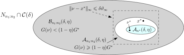
Figure 4.1: The outer ellipse, the set $N_{n_{1}:n_{2}}\cap\mathcal{C}(\delta)$ of count vectors that satisfy the constraints to within tolerance $\delta$, is partitioned into $\mathcal{B}_{n_{1}:n_{2}}$, shown in gray, and $\mathcal{A}_{n_{1}:n_{2}}$, the inner white ellipse. The relationship shown between $\|\nu-x^{\ast}\|_{\infty}\leqslant\delta\vartheta_{\infty}$ and $\mathcal{A}_{n_{1}:n_{2}}(\delta,\eta)$ is not the only one possible. Likewise for $x^{\ast}$ and $\mathcal{A}_{n^{\ast}}(\delta,\eta)$.

4.3.1 Bounds on the concentration threshold

It is useful to know something about how the threshold $\hat{c}$ depends on the solution $x^{\ast},G^{\ast}$ to the MaxGEnt problem and on the parameters $\delta,\varepsilon,\eta$, without having to solve equations. We derive some bounds on $\hat{c}$ with regard to convenience, not tightness.

If $c_{i}\geqslant L_{i}$, then $\hat{c}=\max_{i}c_{i}\geqslant\max_{i}L_{i}$. Hence we have the lower bound

$$\hat{c}\;\geqslant\;\max\Bigl{(}\frac{-\ln(\varepsilon B)}{\eta G^{\ast}},\frac{1}{\delta\vartheta_{\infty}}\Bigr{)},$$ (4.25)

since $c_{1}$ must be bigger than the first term on the r.h.s., and $c_{2}$ equals the second. As intuitively expected, the bound says that the smaller $\delta,\varepsilon$, or $\eta$ are, the more scaling we need. By looking at the expression for $B$ after (4.21), we see that the same holds the farther apart the bounds $s_{1},s_{2}$ on the possible sums are from each other; this accords with intuition, and we discuss it further in Example 4.2.

Next, if $c_{i}\leqslant U_{i}$, then $\max_{i}c_{i}\leqslant\max_{i}U_{i}$. So

$$\hat{c}\;\leqslant\;\max\biggl{(}\frac{2m}{\eta G^{\ast}}\ln\frac{m-\ln(\varepsilon B)}{\eta G^{\ast}}-\frac{\ln(\varepsilon B)}{\eta G^{\ast}},\frac{1}{\delta\vartheta_{\infty}},\sqrt{\frac{\sum_{i=1}^{m}1/(x^{\ast}_{i}-1)}{2\eta G^{\ast}}}\biggr{)},$$ (4.26)

where the expressions on the r.h.s. are upper bounds on $c_{1},c_{2},c_{3}$, respectively, as shown in the Appendix. The upper bound says that the larger $G^{\ast}$ is, the less scaling we need; likewise for the elements of $x^{\ast}$. Both of these implications agree with intuition. Further illustrations of the bounds (4.25) and (4.26) are in Example 4.1.

4.4 Examples

We give two examples. The first continues Example 3.1, illustrates the bounds on the concentration threshold, and points out a, at first sight, surprising behavior of the threshold. The second example illustrates an intuitively-expected relationship between concentration and the bounds $s_{1},s_{2}$.

Example 4.1

Returning to Example 3.1, we find

$$s_{1}=21.5,\;s_{2}=37.5,\;x^{\ast}=(6.591,5.326,13.26,1.120,2.253,2.789),\;s^{\ast}=31.34,\;G^{\ast}=47.53.$$

Thus $\nu^{\ast}=(7,5,14,1,2,3)$ and $n^{\ast}=32$. Also, $\vartheta_{\infty}=2.9$. Table 4.2 shows what happens when the problem data $b$ is scaled by the factor $\hat{c}$ dictated by the given $\delta,\varepsilon,\eta$. [We don’t use a special notation for the quantities appearing in the unscaled vs. the scaled problem, so whenever we write $x^{\ast},\nu^{\ast}$, $b^{E}$, etc. a scaling factor, which could be 1, is implied.]

$\delta\in[0.01,1],\varepsilon=10^{-9}$
$\eta$	$\hat{c}$	$b$	$n_{1}$	$n^{\ast}$	$n_{2}$	$\nu^{\ast}$
0.05	34.48	(362.1,631.0,300.0,137.9)	880	1081	1294	(227,184,457,39,78,96)
0.02	91.27	(958.3,1670,794.0,365.1)	2328	2861	3423	(602,486,1210,102,206,255)
0.01	191.9	(2015,3512,1670,767.7)	4894	6015	7197	(1265,1022,2545,215,433,535)
$\delta\in[0.01,1],\varepsilon=10^{-15}$
0.05	40.25	(422.7,736.6,350.2,161.0)	1027	1262	1510	(266,214,534,45,91,112)
0.02	106.8	(1121.3,1954.3,929.1,427.2)	2724	3347	4005	(703,569,1416,120,241,298)
0.01	222.9	(2340.2,4078.6,1939.0,891.5)	5684	6985	8358	(1469,1187,2955,250,502,622)

Table 4.2: Scaling of the problem of Example 3.1 for the given $\delta,\varepsilon,\eta$.

With respect to the discrete solution, in the first row of Table 4.2 for example, we have $\|x^{\ast}-\nu^{\ast}\|_{\infty}=0.370$. Further, $\nu^{\ast}$ satisfies the equality constraints with tolerance $\|A^{E}\nu^{\ast}-b^{E}\|_{\infty}/\min|b^{E}|=0.0033$ and the inequality constraints with tolerance 0. We see that the scaling factor $\hat{c}$ is quite sensitive to $\eta$ and rather insensitive to $\varepsilon$; this can be surmised from (4.25). One way to interpret the scaling is as a change in the scale of measurement of the data $b$, e.g. a change in the units. Then scaling by a larger factor means choosing more refined units, and the above results show that the concentration increases, as intuitively expected.

With respect to the bounds (4.25) and (4.26) on the threshold $\hat{c}$, for the first row of the table with $\delta=0.01$, they yield $\hat{c}\in[34.48,41.87]$. For $\delta\in[0.02,0.05]$ they yield $\hat{c}\in[25.1,41.87]$. For the second row, the bounds give $\hat{c}\in[62.8,116.2]$ for any $\delta\in[0.01,0.05]$.

Now suppose that the problem data is pre-scaled by 34.5. Then for the first row the bounds say that $\hat{c}\in[1.0,1.0]$, i.e. no further scaling is needed. For the second row, Theorem 4.2 gives $\hat{c}=2.39$ and the bounds give $\hat{c}\in[2.23,2.55]$. So the original problem had a threshold $\hat{c}=91.27$, but when scaled by 34.5, the threshold becomes only $\hat{c}=2.39<\frac{91.27}{34.5}=2.64$. Apparently, unlike the rest of the problem (Proposition 3.2), the concentration threshold does not behave linearly with scaling: $\hat{c}\left(34.5\times\text{problem}\right)<34.5\hat{c}\left(\text{problem}\right)$. The explanation for this at first sight disconcerting behavior is two-fold: first, Theorem 4.2 does not say that $\hat{c}$ is the minimum required scaling factor for a given problem; second, there are many approximations involved in the derivation of $\hat{c}$, and many get better as the size of the problem increases.

Example 4.2

Intuition says that the bounds $s_{1},s_{2}$ on the possible sums of the admissible count vectors have something to do with concentration: if they are wide, concentration should be more difficult to achieve. Suppose that, somehow, the MaxGEnt vector $x^{\ast}$ from which $\nu^{\ast}$ is derived remains fixed; then the wider the range $s_{1},s_{2}$ allowed by the constraints, the larger should be the scaling factor required for $\nu^{\ast}$ to dominate. The bound (4.25) agrees with this, due to the expression for $B$ after (4.21). We now give a simple situation in which the difference between $s_{1}$ and $s_{2}$ can increase while $x^{\ast}$ remains fixed.

Consider a 2-dimensional problem with box constraints $b_{1}\leqslant x_{1}\leqslant b_{2}$, $b_{3}\leqslant x_{2}\leqslant b_{4}$, depicted in Fig. 4.2. Then $s_{1}=b_{1}+b_{3}$, $s_{2}=b_{2}+b_{4}$ and $G$ is maximum at the upper right corner of the box (Proposition 2.3). If we reduce $b_{1},b_{3}$ to $b^{\prime}_{1},b^{\prime}_{3}$, the lower left corner of the box moves down and to the left while the upper right corner remains fixed, as shown in the figure.

Figure 4.2: Reducing $s_{1}$ while leaving $s_{2}$ and $x^{\ast}$ unchanged.

Thus we widen the bounds $s_{1},s_{2}$ while leaving $s^{\ast},G^{\ast}$ unchanged, and the problem with the new box constraints requires more scaling than the original problem. The construction generalizes immediately to $m$ dimensions, see §2.3.

5 Concentration with respect to distance from the MaxGEnt vector

In this section we provide results analogous to those of §4, but with the sets $\mathcal{A},\mathcal{B}$ formulated in terms of the distance of their elements from the optimal vector $x^{\ast}$, as measured by the $\ell_{1}$ norm. This is a more intuitive measure than difference in entropy. There are three main results: Theorems 5.1 and 5.2, analogues of Theorems 4.1 and 4.2, and Theorem 5.3, an optimized version of Theorem 5.2 that does not require specifying a $\delta$. In various places we reuse results and methods from §4, so the presentation here is more succinct.

For given $n$ and $\delta>0$, we want to consider the count vectors in $N_{n}$ that lie in $\mathcal{C}(\delta)$ and whose distance from $x^{\ast}$ is no more than $\vartheta>0$ in $\ell_{1}$ norm, and those that lie in $\mathcal{C}(\delta)$ but are farther from $x^{\ast}$ than $\vartheta$ in $\ell_{1}$ norm. The situation is less straightforward than with frequency/density vectors. First, given two real $m$-vectors, the norm of their difference can never be smaller than the difference of their norms, so it does not make sense to require that this norm be too small. Second, we will be considering norms that can be large numbers, especially after scaling of the problem, so it will not do to consider a fixed-size region around $x^{\ast}$. For these reasons, we define for $\vartheta>0$

$$\begin{gathered}\mathcal{A}_{n}(\delta,\vartheta)\;\triangleq\;\{\nu\in N_{n}\cap\mathcal{C}(\delta),\|\nu-x^{\ast}\|_{1}\leqslant|n-s^{\ast}|+\min(n,s^{\ast})\vartheta\},\\ \mathcal{B}_{n}(\delta,\vartheta)\;\triangleq\;\{\nu\in N_{n}\cap\mathcal{C}(\delta),\|\nu-x^{\ast}\|_{1}>|n-s^{\ast}|+\min(n,s^{\ast})\vartheta\}.\end{gathered}$$ (5.1)

This is more complicated that the definition for frequency vectors in [OG16], but here $\vartheta$ is again a small number $<\;1$. If $n$ were equal to $s^{\ast}$, (5.1) would say that the density vectors $f$ and $\chi^{\ast}$ are such that $\|f-\chi^{\ast}\|_{1}$ is $\leqslant\;\vartheta$ in $\mathcal{A}_{n}$ and $>\;\vartheta$ in $\mathcal{B}_{n}$. In general, (5.1) says that the norm of $\nu-x^{\ast}$ is close to $|n-s^{\ast}|$: if $n\leqslant s^{\ast}$, the bound is $s^{\ast}-(1-\vartheta)n$, and if $n>s^{\ast}$ it is $n-(1-\vartheta)s^{\ast}$.

We will consider the (disjoint) unions of the sets (5.1) over $n\in\{n_{1},\ldots,n_{2}\}$, with $n_{1},n_{2}$ given by (4.2):

$$\begin{gathered}\mathcal{A}_{n_{1}:n_{2}}(\delta,\vartheta)\;\triangleq\;\bigl{\{}\nu\mid\sum_{i}\nu_{i}=n,n_{1}\leqslant n\leqslant n_{2},\nu\in\mathcal{C}(\delta),\|\nu-x^{\ast}\|_{1}\leqslant|n-s^{\ast}|+\min(n,s^{\ast})\vartheta\bigr{\}},\\ \mathcal{B}_{n_{1}:n_{2}}(\delta,\vartheta)\;\triangleq\;\bigl{\{}\nu\mid\sum_{i}\nu_{i}=n,n_{1}\leqslant n\leqslant n_{2},\nu\in\mathcal{C}(\delta),\|\nu-x^{\ast}\|_{1}>|n-s^{\ast}|+\min(n,s^{\ast})\vartheta\bigr{\}}.\end{gathered}$$ (5.2)

For any $\delta,\vartheta$, these two sets partition $N_{n_{1}:n_{2}}\cap\mathcal{C}(\delta)$, the set of count vectors that sum to a number between $n_{1}$ and $n_{2}$ and lie in $\mathcal{C}(\delta)$.

With these definitions, we will establish an analogue of (4.6) in §4: given $\delta,\varepsilon,\vartheta>0$, there is a concentration threshold $\hat{c}=\hat{c}(\delta,\varepsilon,\vartheta)$ s.t. if the problem data $b^{E},b^{I}$ is scaled by any factor $c\geqslant\hat{c}$, then the MaxGEnt count vector $\nu^{\ast}$ is in the set $\mathcal{A}_{n_{1}:n_{2}}(\delta,\vartheta)$ and has at least $1/\varepsilon$ times the realizations of all vectors in the set $\mathcal{B}_{n_{1}:n_{2}}(\delta,\vartheta)$:

$$\nu^{\ast}\in\mathcal{A}_{n_{1}:n_{2}}(\delta,\vartheta)\qquad\text{and}\qquad\frac{\#\nu^{\ast}}{\#\mathcal{B}_{n_{1}:n_{2}}(\delta,\vartheta)}\;\geqslant\;\frac{1}{\varepsilon}.$$ (5.3)

There is one important difference with §4, that here the tolerances $\delta$ and $\vartheta$ cannot be chosen independently of one another, they must obey a certain restriction.

Remark 5.1

$G^{\ast}$ is the maximum of $G$ over the domain $\mathcal{C}(0)$, with no tolerances on the constraints. As we said in §3.1, a tolerance $\delta>0$ widens this domain to $\mathcal{C}(\delta)$, may move the vector that maximizes $G$ from $x^{\ast}(0)$ to $x^{\ast}(\delta)$, and may change the maximum value from $G^{\ast}(0)$ to $G^{\ast}(\delta)$. Here we are looking for concentration in a region of size $\vartheta$ around the point $x^{\ast}$. If $\delta$ is too large, we cannot expect such a region to dominate the count vectors in $\mathcal{C}(\delta)$ w.r.t. the number of realizations, since $x^{\ast}(\delta)$ may even lie inside the set $\mathcal{B}(\delta,\vartheta)$; by Proposition 2.3, it already lies on the ‘boundary’ of $\mathcal{C}(0)$. If $\vartheta$ is given, concentration in $\mathcal{A}(\delta,\vartheta)$ requires an upper bound on the allowable $\delta$; see (5.8) below.

In the setting of §4 there is no limitation on the magnitude of $\delta$ with respect to that of $\eta$. It is perfectly fine if the set $\mathcal{A}_{n}(\delta,\eta)$ contains $\nu$ with $G(\nu)>G^{\ast}(0)$, but not if $\mathcal{B}_{n}(\delta,\eta)$ does. But $\mathcal{B}_{n}(\delta,\eta)$ can’t contain any such $\nu$ by its definition (4.1): if there are any such $\nu$, all of them have to be in $\mathcal{A}_{n}(\delta,\eta)$.

5.1 Realizations of the sets far from the MaxGEnt vector

To bound the number of realizations of $\mathcal{B}_{n_{1}:n_{2}}(\delta,\vartheta)$ we need to show that if $\nu$ is far from $x^{\ast}$, in the $\|\nu-x^{\ast}\|_{1}$ sense, then $G(\nu)$ is far from $G(x^{\ast})$. To simplify the notation, in this section we denote $x^{\ast}(0),\chi^{\ast}(0),G^{\ast}(0)$ simply by $x^{\ast},\chi^{\ast},G^{\ast}$.

We first need an auxiliary relationship between the norm of the difference of two real vectors and the norm of the difference of their normalized versions:

Proposition 5.1

Let $\|\cdot\|$ be any vector norm, such as $\|\cdot\|_{1},\|\cdot\|_{2},\|\cdot\|_{\infty}$ etc. Then for any $x,y\in\mathbb{R}^{m}$ and $\vartheta>0$,

$$\|x-y\|>|\|x\|-\|y\||+\vartheta\quad\Rightarrow\quad\left\|\frac{x}{\|x\|}-\frac{y}{\|y\|}\right\|>\frac{\vartheta}{\min(\|x\|,\|y\|)}.$$

What we want to show about $G(\nu)$ and $G^{\ast}$ follows by taking Lemma 3.1, bounding the divergence term $D(\cdot\|\cdot)$ in terms of the $\ell_{1}$ norm, and then using Proposition 5.1 with the $\ell_{1}$ norm and $\min(\|\nu\|,\|x^{\ast}\|)\vartheta$ in place of $\vartheta$:

Lemma 5.1

Given $\delta\geqslant 0$ and $\vartheta>0$, with the notation of Lemma 3.1, for any count vector $\nu\in\mathcal{C}(\delta)$ with sum $n$,

$$\|\nu-x^{\ast}\|_{1}>|n-s^{\ast}|+\min(n,s^{\ast})\vartheta\quad\Rightarrow\quad G(\nu)\;\leqslant\;G^{\ast}+\Lambda^{\ast}\delta-\gamma^{\ast}\vartheta^{2}n$$

where

$$\gamma^{\ast}\triangleq\frac{1}{4(1-2\beta^{\ast})}\ln\frac{1-\beta^{\ast}}{\beta^{\ast}},\quad\beta^{\ast}\triangleq\max_{I\subset\{1,\ldots,m\}}\min\Bigl{(}\sum_{i\in I}\chi^{\ast}_{i},1-\sum_{i\in I}\chi^{\ast}_{i}\Bigr{)}.$$

In general, $\gamma^{\ast}\geqslant\frac{1}{2}$ and $\frac{1-\chi^{\ast}_{\max}}{2}\leqslant\beta^{\ast}\leqslant\frac{1}{2}$. If $\beta^{\ast}=1/2$, $\gamma^{\ast}\triangleq 1/2$.

The bound on the divergence that we used above, $D(p\|q)\geqslant\gamma(q)\|p-q\|_{1}^{2}$, is due to [OW05]. The closeness of the number $\beta(q)$ to $1/2$ can be thought of as measuring how far away the density vector $q$ is from having a partition. [BHK14] is also relevant here, as the authors study $\inf_{p}D(p\|q)$ subject to $\|p-q\|_{1}\geqslant\ell$. They refer to $1-\beta\geqslant 1/2$, where $\beta$ is as in Lemma 5.1, as the “balance coefficient”. Their Theorem 1b provides an exact value for $\inf_{p}D(p\|q)$ as a function of $1-\beta$, $q$, and $\ell$, valid for $\ell\leqslant 4(1/2-\beta)$; this could be used in Lemma 5.1, at the expense of an additional condition between, in our notation, $\vartheta$ and $\beta^{\ast}$. They also show that $\beta\geqslant 1/2-q_{\max}/2$, where $q_{\max}$ is the largest element of $q$, a result which we have incorporated into Lemma 5.1.

We can now proceed to find an upper bound on $\#\mathcal{B}_{n_{1}:n_{2}}(\delta,\vartheta)$. Beginning with $\#\mathcal{B}_{n}(\delta,\vartheta)$, by (5.1) and (4.7)

$$\#\mathcal{B}_{n}(\delta,\vartheta)\;\leqslant\sum_{\text{\scriptsize{$\begin{array}[]{c}\nu\in N_{n}\cap\mathcal{C}(\delta)\\ \|\nu-x^{\ast}\|_{1}>|n-s^{\ast}|+\min(n,s^{\ast})\vartheta\end{array}$}}}S(\nu)e^{G(\nu)}.$$

Applying Lemma 5.1 to $G(\nu)$ and, similarly to what we did in §4.2, ignoring the condition involving the norm in the sum as well as the intersection with $\mathcal{C}(\delta)$,

$$\#\mathcal{B}_{n}(\delta,\vartheta)\;\leqslant\;e^{G^{\ast}+\Lambda^{\ast}\delta-\gamma^{\ast}\vartheta^{2}n}\;\sum_{\nu\in N_{n}}S(\nu).$$

The sum above is identical to that in the expression for $\#\mathcal{B}_{n}(\delta,\eta)$ given at the beginning of §4.2, so following the development that led to (4.15),

$$\#\mathcal{B}_{n}(\delta,\vartheta)\;\leqslant\;\sqrt{2\pi/n}\;\frac{(n/2)^{m/2}}{\Gamma(m/2)}\bigl{(}1+\sqrt{m/n}\bigr{)}^{m}e^{G^{\ast}+\Lambda^{\ast}\delta-\gamma^{\ast}\vartheta^{2}n}.$$

Compare with (4.15). Consequently,

$$\#\mathcal{B}_{n_{1}:n_{2}}(\delta,\vartheta)\;=\;\sum_{n_{1}\leqslant n\leqslant n_{2}}\#\mathcal{B}_{n}(\delta,\vartheta)$$ (5.4)

$$\qquad\leqslant\;\frac{\sqrt{2\pi}}{2^{m/2}\Gamma(m/2)}\;e^{G^{\ast}+\Lambda^{\ast}\delta}\sum_{n_{1}\leqslant n\leqslant n_{2}}\frac{1}{\sqrt{n}}\bigl{(}\sqrt{m}+\sqrt{n}\bigr{)}^{m}\,e^{-\gamma^{\ast}\vartheta^{2}n}$$

$$\qquad\leqslant\;\frac{\sqrt{2\pi}}{2^{m/2}\Gamma(m/2)}\,e^{G^{\ast}+\Lambda^{\ast}\delta}$$

$$\hskip 40.00006pt\frac{2}{(m+1)}\Bigl{(}\bigl{(}\sqrt{s_{2}+2}+\sqrt{m}\bigr{)}^{m+1}\,e^{-\gamma^{\ast}\vartheta^{2}(s^{\ast}+1)}+\bigl{(}\sqrt{s^{\ast}+2}+\sqrt{m}\bigr{)}^{m+1}\,e^{-\gamma^{\ast}\vartheta^{2}s_{1}}\Bigr{)}$$

where the inequality implied in the last line is derived in the Appendix. This bound on $\#\mathcal{B}_{n_{1}:n_{2}}(\delta,\vartheta)$ is to be compared with the bound (4.16) on $\#\mathcal{B}_{n_{1}:n_{2}}(\delta,\eta)$.

Combining (4.11) with (5.4) we obtain a lower bound on the ratio of numbers of realizations analogous to that of Theorem 4.1:

Theorem 5.1

Given structure matrices $A^{E},A^{I}$ and data vectors $b^{E},b^{I}$, let $(x^{\ast},s_{1},s_{2})$ be the optimal solution of problem (1.1). Assume that $x^{\ast}>\boldsymbol{1}$; recall Remark 4.2. Then for any $\delta,\varepsilon,\vartheta>0$,

$$\frac{\#\nu^{\ast}}{\#\mathcal{B}_{n_{1}:n_{2}}(\delta,\vartheta)}\;>\;\frac{(m+1)\Gamma(m/2)e^{-m/12}}{2\pi^{m/2}}\frac{C_{2}(x^{\ast})C_{4}(x^{\ast})}{C^{\prime}_{3}(s^{\ast},s_{1},s_{2})}\;\;e^{\gamma^{\ast}\vartheta^{2}s_{1}-\Lambda^{\ast}\delta},$$

where the constants $C_{2}(x^{\ast}),C_{4}(x^{\ast})$ are the same as in (4.17),

$$C^{\prime}_{3}(s^{\ast},s_{1},s_{2})\;=\;\left(\sqrt{s_{2}+2}+\sqrt{m}\right)^{m+1}e^{-\gamma^{\ast}\vartheta^{2}(s^{\ast}-s_{1}+1)}+\left(\sqrt{s^{\ast}+2}+\sqrt{m}\right)^{m+1},$$

and $\Lambda^{\ast},\gamma^{\ast}$ have been defined in Lemmas 3.1 and 5.1 respectively.

The lower bound will not be useful if the exponent $\gamma^{\ast}\vartheta^{2}s_{1}-\Lambda^{\ast}\delta$ is not positive. We elaborate on this in §5.2. Also, like Theorem 4.1, the theorem says nothing about how large the bound is for a given problem. This is the job of Theorem 5.2.

5.2 Scaling and concentration around the MaxGEnt count vector

As we did in §4.3, we now investigate what happens to the lower bound of Theorem 5.1 when the problem data $b$ is scaled by a factor $c\geqslant 1$. The end results are the concentration Theorems 5.2 and 5.3 below.

Table 4.1 described how scaling the data affects the quantities appearing in the bound, except for $\Lambda^{\ast}$, which is new to §5. Scaling $b$ has the effect $x^{\ast}\mapsto cx^{\ast}$, and from (2.4) in §2.4 we see that the Lagrange multipliers remain unchanged. Then the definition of $\Lambda^{\ast}$ in Lemma 3.1 shows that the end result of scaling is $\Lambda^{\ast}\mapsto c\Lambda^{\ast}$. This and $s_{1}\mapsto cs_{1}$ imply that scaling by $c$ multiplies the exponent $\gamma^{\ast}\vartheta^{2}s_{1}-\Lambda^{\ast}\delta$ in Theorem 5.1 by $c$. The effect of scaling on $C_{2}$ and $C_{4}$ is given by (4.18) and (4.20), and finally

$$\begin{array}[]{l}C^{\prime}_{3}(cs^{\ast},cs_{1},cs_{2})\;<\\ \qquad c^{\frac{m+1}{2}}\bigl{(}(\sqrt{s_{2}+2}+\sqrt{m})^{m+1}\,e^{-\gamma^{\ast}\vartheta^{2}}e^{-c\gamma^{\ast}\vartheta^{2}(s^{\ast}-s_{1})}+(\sqrt{s^{\ast}+2}+\sqrt{m})^{m+1}\bigr{)}\\ \qquad\leqslant\;c^{\frac{m+1}{2}}\bigl{(}(\sqrt{s_{2}+2}+\sqrt{m})^{m+1}e^{-\gamma^{\ast}\vartheta^{2}(s^{\ast}-s_{1}+1)}+(\sqrt{s^{\ast}+2}+\sqrt{m})^{m+1}\bigr{)}\\ \qquad\triangleq\;c^{\frac{m+1}{2}}C^{\prime\prime}_{3},\end{array}$$ (5.5)

where the 2nd inequality follows from $c\geqslant 1$. In conclusion, when the data $b$ is scaled by the factor $c\geqslant 1$, Theorem 5.1 says that if $x^{\ast}>\boldsymbol{1}$, then

$$\frac{\#\nu^{\ast}}{\#\mathcal{B}_{n_{1}:n_{2}}(\delta,\vartheta)}\;>\;\frac{B^{\prime}}{C^{\prime\prime}_{3}}c^{-m}e^{(2\gamma^{\ast}\vartheta^{2}s_{1}-\Lambda^{\ast}\delta)c},$$ (5.6)

where $C^{\prime\prime}_{3}$ is defined in (5.5) and

$$B^{\prime}\;\triangleq\;\frac{(m+1)\Gamma(m/2)e^{-m/12}}{2\pi^{m/2}}\sqrt{s^{\ast}}e^{-\frac{1}{2}\sum_{i=1}^{m}\frac{1}{x^{\ast}_{i}-1}}\prod_{1\leqslant i\leqslant m}\frac{\chi^{\ast}_{i}}{\sqrt{x^{\ast}_{i}+1}}.$$ (5.7)

(5.6) and (5.7) are to be compared with (4.21).

Recalling Remark 5.1, an important consequence of (5.6) is that if concentration is to occur the tolerances $\delta$ and $\vartheta$ must satisfy

$$\vartheta^{2}\;>\;\frac{\Lambda^{\ast}}{2\gamma^{\ast}s_{1}}\delta.$$ (5.8)

This can be ensured by choosing small enough $\delta$ for the given $\vartheta$, or large enough $\vartheta$ for the given $\delta$. (The results of this paper do not immediately translate to the frequency vector case, but (5.8) can be compared with the similar condition in Theorem IV.2 of [OG16].)

By (5.6), the concentration statement (5.3) will hold if the scaling factor $c$ is such that

$$(2\gamma^{\ast}\vartheta^{2}s_{1}-\Lambda^{\ast}\delta)c-m\ln c\;\geqslant\;\ln\frac{C^{\prime\prime}_{3}}{\varepsilon B^{\prime}}.$$ (5.9)

This inequality is of the same form as (4.22), and will hold for all $c$ greater than the larger of the two roots of the equality version of it.

As in §4.3, we also need $\nu^{\ast}$ to be in the set $\mathcal{A}_{n_{1}:n_{2}}(\delta,\vartheta)$ of (5.2), more specifically in $\mathcal{A}_{n^{\ast}}(\delta,\vartheta)$. For this, we must first have $\nu^{\ast}\in\mathcal{C}(\delta)$; this is ensured by $c\geqslant c_{2}$, with $c_{2}$ as in (4.23). Second, by the definition (5.1) of $\mathcal{A}_{n}(\delta,\vartheta)$, we need $\|\nu^{\ast}-x^{\ast}\|_{1}\leqslant|n^{\ast}-s^{\ast}|+\min(n^{\ast},s^{\ast})\vartheta$; by Proposition 3.4 this will hold if $\vartheta\geqslant(3m/4+1)/(cs^{\ast})$.

We have now established the desired analogue of Theorem 4.2, and proved the statement GC of §1, in terms of distance from the MaxGEnt vector $x^{\ast}$:

Theorem 5.2

With the same conditions as in Theorem 5.1, suppose that the tolerances $\delta,\vartheta$ satisfy (5.8), where $\Lambda^{\ast},\gamma^{\ast}$ have been defined in Lemmas 3.1 and 5.1. Let

$$c_{1}\;\triangleq\;\frac{3m/4+1}{\vartheta s^{\ast}},\quad c_{2}\;\triangleq\;\frac{1}{\delta\vartheta_{\infty}},$$

and given $\varepsilon>0$, let $c_{3}$ be the largest root $c$ of the equality version of (5.9). Finally, define the concentration threshold

$$\hat{c}\;\triangleq\;\max(c_{1},c_{2},c_{3}).$$

Then when the data $b^{E},b^{I}$ is scaled by any $c\geqslant\hat{c}$, the MaxGEnt count vector $\nu^{\ast}$ of Definition 3.1 belongs to the set $\mathcal{A}_{n_{1}:n_{2}}(\delta,\vartheta)$ of (5.2), specifically to $\mathcal{A}_{n^{\ast}}(\delta,\vartheta)$, and is such that

$$\frac{\#\nu^{\ast}}{\#\mathcal{B}_{n_{1}:n_{2}}(\delta,\vartheta)}\geqslant\frac{1}{\varepsilon}\quad\text{and}\quad\frac{\#\mathcal{A}_{n_{1}:n_{2}}(\delta,\vartheta)}{\#(N_{n_{1}:n_{2}}\cap\mathcal{C}(\delta))}>1-\varepsilon.$$

The second inequality in the claim of the theorem follows from the first by (4.5) in §4, which holds whether the sets $\mathcal{A}_{n_{1}:n_{2}}$ and $\mathcal{B}_{n_{1}:n_{2}}$ are defined as they were in §4 or as they were defined here. As in Theorem 4.2, the constraint information $A^{E},b^{E},A^{I},b^{I}$ appears implicitly in Theorem 5.2, via $s_{1},s_{2}$, and $\vartheta_{\infty}$. Bounds on the concentration threshold can be derived similarly to §4.3.1.

Finally, Fig. 5.1 depicts the various sets involved in the definition of the threshold $\hat{c}$ appearing in the theorem.

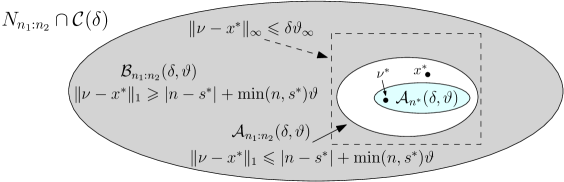
Figure 5.1: Concentration around $\nu^{\ast}$ w.r.t. $\ell_{1}$ norm. The MaxGEnt vector $\nu^{\ast}$ has $1/\varepsilon$ times more realizations than the entire set $\mathcal{B}_{n_{1}:n_{2}}(\delta,\vartheta)$, shown in gray. The relationship we show between $\|\nu-x^{\ast}\|_{\infty}\leqslant\delta\vartheta_{\infty}$ and $\mathcal{A}_{n_{1}:n_{2}}(\delta,\vartheta)$ is not the only one possible; likewise for $x^{\ast}$ and $\mathcal{A}_{n^{\ast}}(\delta,\vartheta)$.

From the definition of $\hat{c}$ in Theorem 5.2 we see that as $\delta$ increases, the constants $c_{2}$ and $c_{3}$ behave in opposite ways: $c_{2}$ decreases but $c_{3}$ increases. If one cares only about the tolerances $\varepsilon$ and $\vartheta$, and does not care to specify a particular $\delta$, this opens the possibility of reducing $\hat{c}$ by choosing $\delta$ so as to minimize the largest of $c_{2},c_{3}$:

Theorem 5.3

Given $\varepsilon,\vartheta$, suppose that

$$\Lambda^{\ast}\geqslant m\vartheta_{\infty}\quad\text{and}\quad\vartheta^{2}\;<\;\frac{\Lambda^{\ast}\sqrt{s^{\ast}/m+1}}{\gamma^{\ast}\vartheta_{\infty}s_{1}}\frac{1}{\varepsilon^{1/m}},$$

where the various quantities are as in Theorem 5.2. If so, the equation for $\delta$

$$\frac{2\gamma^{\ast}\vartheta^{2}s_{1}}{\vartheta_{\infty}}\frac{1}{\delta}+m\ln\delta\;=\;\ln\frac{C^{\prime\prime}_{3}}{\varepsilon B^{\prime}}+\frac{\Lambda^{\ast}}{\vartheta_{\infty}}-m\ln\vartheta_{\infty}$$

has a root $\delta_{0}\in\bigl{(}0,2\gamma^{\ast}\vartheta^{2}s_{1}/\Lambda^{\ast}\bigr{]}$, and we define

$$\hat{c}\;\triangleq\;\max\Bigl{(}\frac{1}{\delta_{0}\vartheta_{\infty}},\frac{3m/4+1}{\vartheta s^{\ast}}\Bigr{)}.$$

Then when the data $b^{E},b^{I}$ is scaled by any $c\geqslant\hat{c}$, the MaxGEnt count vector $\nu^{\ast}$ of Definition 3.1 belongs to the set $\mathcal{A}_{n^{\ast}}(\delta_{0},\vartheta)$ of (5.1), and is such that

$$\frac{\#\nu^{\ast}}{\#\mathcal{B}_{n_{1}:n_{2}}(\delta_{0},\vartheta)}\geqslant\frac{1}{\varepsilon}\quad\text{and}\quad\frac{\#\mathcal{A}_{n_{1}:n_{2}}(\delta_{0},\vartheta)}{\#(N_{n_{1}:n_{2}}\cap\mathcal{C}(\delta_{0}))}>1-\varepsilon.$$

In this situation a simple lower bound on the concentration threshold $\hat{c}$ is

$$\hat{c}\;\geqslant\;\max\left(\frac{H(\chi^{\ast})}{2\gamma^{\ast}}\frac{1}{\vartheta_{\infty}\vartheta^{2}},\frac{3m}{4s^{\ast}\vartheta}\right)$$ (5.10)

where for the first expression we used the upper bound on $\delta_{0}$ and $\Lambda^{\ast}\geqslant s^{\ast}H(\chi^{\ast})$. The ratio $H(\chi^{\ast})/\gamma^{\ast}$ is small for imbalanced distributions $\chi^{\ast}$, e.g. with a single dominant element, in which case $\gamma^{\ast}$ is large, and approaches $2\ln m$ for perfectly balanced ones. The bound (5.10) says that $\hat{c}$ increases with $\vartheta^{-2}$, and this can be seen in Example 5.2 below.

5.3 Examples

The first two examples illustrate Theorems 5.2 and 5.3, while the third illustrates the removal of 0s from the solution mentioned in §2.4 and the ‘boundary’ case in which the MaxGEnt vector $x^{\ast}$ sums to the maximum allowable $s^{\ast}=s_{2}$.

Example 5.1

We return to Example 4.1. Recall that

$$s_{1}=21.5,\;s_{2}=37.5,\;x^{\ast}=(6.591,5.326,13.26,1.120,2.253,2.789),\;s^{\ast}=31.34,\;G^{\ast}=47.53.$$

We have $\vartheta_{\infty}=2.9$, $\gamma^{\ast}=0.5$, and $\Lambda^{\ast}=G^{\ast}=47.53$. The constraint (5.8) on $\delta$ and $\vartheta$ is $\vartheta^{2}>1.864\delta$. This means that if we want small $\vartheta$, we must have a correspondingly small $\delta$, as we commented after (5.8). Table 5.1 lists various values of $\hat{c}(\delta,\varepsilon,\vartheta)$ obtained from Theorem 5.2.

$\hat{c}$ $\delta$ $\vartheta$ $\varepsilon=10^{-9}$ $\varepsilon=10^{-15}$ 0.001 0.08 862.7 989.2 $10^{-4}$ 3448 3448 $10^{-5}$ 34483 34483 0.001 0.07 1322 1511 $10^{-4}$ 3448 3448 $10^{-5}$ 34483 34483 0.001 0.06 2392 2722 $10^{-4}$ 3448 3448 $10^{-5}$ 34483 34483 $10^{-4}$ 0.05 3448 3448 $10^{-5}$ 34483 34483 $10^{-5}$ 0.03 34483 34483 0.01 $60376$ $67351$ 0.008 $111472$ $123967$

Table 5.1: Scaling of the problem of Example 4.1 for the given $\delta,\varepsilon,\vartheta$. The threshold $\hat{c}$ does not behave smoothly because of the $\max()$ in Theorem 5.2.

Example 5.2

Consider the same data as in Table 5.1, but with only $\varepsilon,\vartheta$ specified; we don’t care about a particular $\delta$, as long as it ensures that $\nu^{\ast}\in\mathcal{A}_{n^{\ast}}(\delta,\vartheta)$. With $\delta$ chosen automatically by Theorem 5.3, Table 5.2 below shows that the concentration threshold $\hat{c}$ is significantly reduced.

	$\hat{c}$
$\vartheta$	$\varepsilon=10^{-9}$	$\varepsilon=10^{-15}$
0.08	704.4	793.4
0.07	933.5	1050
0.06	1292	1450
0.05	1896	2124
0.04	3032	3387
0.03	5548	6178
0.01	$55345$	60991
0.008	88189	97004

Table 5.2: The threshold $\hat{c}$ for given $\varepsilon,\vartheta$ with optimal selection of $\delta=\delta_{0}$. Compare with Table 5.1.

The variation of $\hat{c}$ with $\vartheta^{-2}$ implied by the lower bound (5.10) is evident.

Example 5.3

Fig. 5.2 shows four cities connected by road segments. We assume that vehicles travelling from one city to another follow the most direct route, and that there is no traffic from a city to itself.

Figure 5.2: Four cities connected by (bidirectional) road segments. Arrows indicate the constrained directions.

The number of vehicles in city $i$ is known, which puts upper bounds on the number that leaves each city; also, from observations we have lower bounds on the number of vehicles on the road segments $2\rightarrow 3$, $3\rightarrow 1$, and $3\rightarrow 4$. From this information we want to infer how many vehicles travel from city $i$ to city $j$, i.e. infer the $4\times 4$ matrix of counts

$$v=\left(\begin{array}[]{cccc}0&v_{12}&v_{13}&v_{14}\\ v_{21}&0&v_{23}&v_{24}\\ v_{31}&v_{32}&0&v_{34}\\ v_{41}&v_{42}&v_{43}&0\end{array}\right).$$

So suppose the constraints on $v$ are

$$v_{ii}=0,\quad\sum_{j}v_{ij}\leqslant 100,120,80,90,\quad v_{23}+v_{24}\geqslant 80,\quad v_{31}+v_{41}\geqslant 59,\quad v_{14}+v_{24}+v_{34}\geqslant 70,$$

where the last three reflect the “direct route” assumption. Then we have $s_{1}=139,s_{2}=390$. We define the 12-element vector $x$ for the MaxGEnt method as $(v_{12},v_{13},v_{14},v_{21},v_{23},v_{24},\allowbreak\ldots,v_{43})$. [Note that if we knew that all vehicles in a city leave the city, then we could define a frequency matrix by dividing the matrix $v$ by $100+\cdots+90$ and thus formulate a MaxEnt problem.] The MaxGEnt solution is

$$v^{\ast}\;=\;\left(\begin{array}[]{cccc}0&33.333&33.333&33.333\\ 40.0&0&40.0&40.0\\ 27.765&26.118&0&26.118\\ 31.235&29.382&29.382&0\end{array}\right)$$

with sum $s^{\ast}=s_{2}=390$ and maximum generalized entropy $G^{\ast}=964.62$, $\Lambda^{\ast}=971.84$, $\gamma^{\ast}=0.5$. So here we have the boundary case in which the sum of $x^{\ast}$ is the maximum possible. (Problems involving matrices subject to constraints of the above type, for which analytical solutions are possible, were studied in [Oik12].)

Applying Theorem 5.3 with $\vartheta=0.04,\varepsilon=10^{-15}$ the ‘optimal’ $\delta$ is $\delta_{0}\approx 2.02\cdot 10^{-5}$ and yields the threshold $\hat{c}=837.9$. Using a scaling factor $c=838$ on $v^{\ast}$ results in the integral matrix

$$\nu^{\ast}\;=\;\left(\begin{array}[]{cccc}0&27394&27393&27393\\ 33520&0&33520&33520\\ 23267&21887&0&21887\\ \mathrm{26175}&24622&24622&0\end{array}\right)$$

with sum $n^{\ast}=326820\in[116842,326820]$. This matrix has at least $10^{15}$ times the number of realizations of the entire set $\mathcal{B}_{116842:326820}(2.02\cdot 10^{-5},0.04)$ defined in (5.2). To gain some appreciation of what this means, it is not easy to determine the size of this set, but just the particular subset of it

$$\mathcal{B}_{326819}(0,0.04)=\{\nu\in\mathcal{C}(0),\|\nu-x^{\ast}\|_{1}>13073\}$$

contains at least $2.012\cdot 10^{37}$ elements. For comparison, the whole of $\mathcal{C}(0)$ has $2.394\cdot 10^{54}$ elements. (We compute these numbers with the barvinok software, [VWBC05]. For $\mathcal{B}_{326819}$ we get a lower bound by using the stronger constraint $|\nu_{1}-x^{\ast}_{1}|>13072$ in place of $\|\nu-x^{\ast}\|_{1}>13073$, which is harder to express.)

6 Conclusion

We demonstrated an extension of the phenomenon of entropy concentration, hitherto known to apply to probability or frequency vectors, to the realm of count vectors, whose elements are natural numbers. This required introducing a new entropy function in which the sum of the count vector plays a role. Still, like the Shannon entropy, this generalized entropy can be viewed combinatorially as an approximation to the log of a multinomial coefficient. Our derivations are carried out in a fully discrete, finite, non-asymptotic framework, do not involve any probabilities, and all of the objects about which we make any claims are fully constructible. This discrete, combinatorial setting is an attempt to reduce the phenomenon of entropy concentration to its essence. We believe that this concentration phenomenon supports viewing the maximization of our generalized entropy as a compatible extension of the well-known MaxEnt method of inference.

Acknowledgments

Thanks to Peter Grünwald for his comments on a previous version of the manuscript, and for many useful discussions on the subject.

Appendix A Proofs

Proof of Proposition 2.1

Given a $y\geqslant x$, $y$ can be reached from $x$ by a sequence of steps each of which increases a single coordinate, and the value of $G$ increases at each step because all its partial derivatives are positive. (The derivatives are 0 only at points $x$ that consist of a single non-zero element; a direct proof can be given for that case.)

For a more formal proof, we note that the directional derivative $G^{\prime}(\xi;u)$ of $G$ at any point $\xi$ is $\geqslant\;0$ in any direction $u\geqslant 0$: $G^{\prime}(\xi;u)=\nabla G(\xi)\cdot u=\sum_{i}u_{i}\ln\frac{\xi_{1}+\cdots+\xi_{m}}{\xi_{i}}$. So any move away from $\xi$ in a direction $u\geqslant 0$ will increase $G$. More precisely, by the mean value theorem, for any $y$ that can be written as $x+u$ for some $u\geqslant 0$, there is a $\xi$ on the line segment from $x$ to $x+u$ s.t. $G(x+u)-G(x)=\nabla G(\xi)\cdot u\geqslant 0$. Finally, if some element of $u$ is strictly positive, then $\nabla G(\xi)\cdot u>0$.

Proof of Proposition 2.2

1. To establish concavity it suffices to show that $\nabla^{2}G(x)$, the Hessian of $G$, is negative semi-definite. We find

   $$\nabla^{2}G(x)\;=\;\frac{1}{x_{1}+\cdots+x_{m}}U_{m}-\operatorname{diag}\Bigl{(}\frac{1}{x_{1}},\ldots,\frac{1}{x_{m}}\Bigr{)},$$ (A.1)

   where $U_{m}$ is a $m\times m$ matrix all of whose entries are 1. Given $x$, for an arbitrary $y=(y_{1},\ldots,y_{m})$ we must have $y^{T}\nabla^{2}G(x)y\leqslant 0$. To show this, first write $\nabla^{2}G(x)$ as

   $$\nabla^{2}G(x)\;=\;\frac{1}{x_{1}+\cdots+x_{m}}\Bigl{(}U_{m}-\operatorname{diag}\Bigl{(}\frac{x_{1}+\cdots+x_{m}}{x_{1}},\ldots,\frac{x_{1}+\cdots+x_{m}}{x_{m}}\Bigr{)}\Bigr{)}.$$

   Now define $\xi_{i}=x_{i}/(x_{1}+\cdots+x_{m})$. Then $y^{T}\nabla^{2}G(x)y\leqslant 0$ is equivalent to

   $$(y_{1}+\cdots+y_{m})^{2}\;\leqslant\;y_{1}^{2}/\xi_{1}+\cdots+y_{m}^{2}/\xi_{m},$$ (A.2)

   where the $\xi_{i}$ are $\geqslant 0$ and sum to 1. But for fixed $y$, $y^{2}_{1}/\xi_{1}+\cdots+y^{2}_{m}/\xi_{m}$ is a convex function of $\xi=(\xi_{1},\ldots,\xi_{m})$ over the domain $\xi\succ 0$, and its minimum under the constraint $\xi_{1}+\cdots+\xi_{m}=1$ occurs at $\xi_{i}=y_{i}/(y_{1}+\cdots+y_{m})$. So the least value of the r.h.s. of (A.2) as a function of $\xi_{1},\ldots,\xi_{m}$ is $(y_{1}+\cdots+y_{m})^{2}$, and this establishes (A.2).

   For a given $x$ we see that $y^{T}\nabla^{2}G(x)y$ is 0 exactly at points $y$ such that for all $i$, $x_{i}/\sum_{j}x_{j}=y_{i}/\sum_{j}y_{j}$, i.e. iff $y=cx$ for some $c\in\mathbb{R}$.

2. The fact that the Hessian fails to be negative definite does not imply that $G$ is not strictly concave; negative definiteness is a sufficient, but not a necessary condition for strict concavity.

   It can be seen that $G$ is not strictly concave because of the scaling or homogeneity property P9 in §2.1: consider the distinct points $x$ and $y=2x$; strict concavity would require $G((x+y)/2)>G(x)/2+G(y)/2$, which is not true.

3. Proposition 1.1.2 in Chapter IV of [HUL96] says that a function $F(x)$ is strongly convex on a convex set $C$ with modulus $\gamma>0$ iff the modified function $F(x)-\frac{1}{2}\gamma\|x\|_{2}^{2}$ is convex on $C$. Applying this to our function $G$, by the proof carried out in part 1, we would have to show that given any $x\in\mathbb{R}_{+}^{m}$, for all $y\in\mathbb{R}_{+}^{m}$

   $$(y_{1}+\cdots+y_{m})^{2}-(y^{2}_{1}/\xi_{1}+\cdots+y^{2}_{m}/\xi_{m})+\gamma(y^{2}_{1}+\cdots+y^{2}_{m})\;\leqslant\;0$$

   for the chosen modulus $\gamma>0$. But for any $x$ and any $\gamma>0$, this condition is false at the point $y=\gamma x$.

4. By Definition 1.1.1 in [HUL96] Ch. V, §1.1, a convex and positively homogeneous function $F$ defined over the extended real numbers $\mathbb{R}\cup\{\pm\infty\}$ is sublinear. If we define $G(\cdot)$ over all of $\mathbb{R}^{m}$ by setting $G(x_{1},\ldots,x_{m})=-\infty$ if any $x_{i}$ is negative, the above statement applies to $F=-G$. Finally, a sublinear function has the property $F(\alpha x+\beta y)\leqslant\alpha F(x)+\beta F(y)$.

Proof of Lemma 2.1

By (2.2), if $\|x-y\|_{\infty}\leqslant\zeta$ we have $G(y)\geqslant G(x-\boldsymbol{\zeta})$. Now we expand $G(x-\boldsymbol{\zeta})$ in a Taylor series around $x$. Since $G(\cdot)$ is a twice-differentiable function on the open set $x>\boldsymbol{\zeta}$, if $x,x^{\prime}$ are two points in this set, then there is a $\tilde{x}=(1-\alpha)x+\alpha x^{\prime}$ with $\alpha\in[0,1]$, such that

$$G(x^{\prime})\;=\;G(x)+\nabla G(x)\cdot(x^{\prime}-x)+\frac{1}{2}(x^{\prime}-x)^{T}\cdot\nabla^{2}G(\tilde{x})\cdot(x^{\prime}-x)$$

(Theorem 12.14 of [Apo74]). Set $x^{\prime}=x-\boldsymbol{\zeta}$, so $\tilde{x}=x-\alpha\zeta$. Noting that

$$\nabla G(x) =\Bigl{(}\ln\frac{x_{1}+\cdots+x_{m}}{x_{1}},\ldots,\ln\frac{x_{1}+\cdots+x_{m}}{x_{m}}\Bigr{)},$$

$$\nabla^{2}G(\tilde{x}) =\frac{1}{\tilde{x}_{1}+\cdots+\tilde{x}_{m}}U_{m}-\mathrm{diag}\Bigl{(}\frac{1}{\tilde{x}_{1}},\ldots,\frac{1}{\tilde{x}_{m}}\Bigr{)},$$

$$(x^{\prime}-x)^{T}\cdot\nabla^{2}G(\tilde{x})\cdot(x^{\prime}-x) =\zeta^{2}\sum_{i}\Bigl{(}\frac{m^{2}}{\tilde{x}_{1}+\cdots+\tilde{x}_{m}}-\frac{1}{\tilde{x}_{i}}\Bigr{)},$$

where the second equality is (A.1) in the proof of Proposition 2.2, we find that for any $x>\boldsymbol{\zeta}$

$$G(x-\boldsymbol{\zeta})\;=\;G(x)-\zeta\sum_{i}\ln\frac{x_{1}+\cdots+x_{m}}{x_{i}}-\frac{1}{2}\zeta^{2}\Bigl{(}\sum_{i}\frac{1}{x_{i}-\alpha\zeta}-\frac{m}{\|x\|_{1}/m-\alpha\zeta}\Bigr{)},$$ (A.3)

where we know that the sum of the $\zeta$ and the $\zeta^{2}$ terms on the right is negative. [We chose to expand around the point $x-\boldsymbol{\zeta}$ because then the sign of the terms $\nabla G(x)\cdot\boldsymbol{\zeta}$ and $\boldsymbol{\zeta}^{T}\cdot\nabla^{2}G(\tilde{x})\cdot\boldsymbol{\zeta}$ is known.] Now for fixed $x$ define the function

$$g(\alpha,\zeta)\;\triangleq\sum_{1\leqslant i\leqslant m}\frac{1}{x_{i}-\alpha\zeta}-\frac{m}{\|x\|_{1}/m-\alpha\zeta},\quad\alpha\in[0,1],\zeta\geqslant 0,\;x>\boldsymbol{\zeta}.$$ (A.4)

This function is $\geqslant\;0$ and increasing with $\alpha$. To see that $g(\alpha,\zeta)\geqslant 0$, set $u_{i}=x_{i}-\alpha\zeta$ so that $\|x\|_{1}/m-\alpha\zeta$ becomes the arithmetic mean $\bar{u}$ of the $u_{i}$; then use a fundamental property of the power means: for any $u\geqslant 0$, and any weights $w_{i}$ summing to 1,

$$\biggl{(}\sum_{i}w_{i}u_{i}^{-k}\biggr{)}^{-1/k}\;\leqslant\;\sum_{i}w_{i}u_{i},\qquad k\geqslant 1$$ (A.5)

(see [HLP97], Theorem 16). The desired result follows by choosing all $w_{i}=1/m$. To show that $g(\alpha,\zeta)$ increases with $\alpha$,

$$\frac{\partial g}{\partial\alpha}=\sum_{i}\frac{\zeta}{(x_{i}-\alpha\zeta)^{2}}-\frac{m\zeta}{(\|x\|_{1}/m-\alpha\zeta)^{2}}$$

and this is always $\geqslant\;0$ by the same power means technique (A.5). [Similarly, $\partial^{2}g/\partial\alpha^{2}\geqslant 0$, so $g(\alpha,\zeta)$ is a convex function of $\alpha$.] We therefore see that for any $\zeta\geqslant 0$

$$\min_{\alpha\in[0,1]}g(\alpha,\zeta)=g(0,\zeta)\qquad\text{and}\qquad\max_{\alpha\in[0,1]}g(\alpha,\zeta)=g(1,\zeta).$$ (A.6)

It now follows from $G(y)\geqslant G(x-\boldsymbol{\zeta})$, (A.3), and (A.6) that for any $x>\boldsymbol{\zeta}$ and any $y$ s.t. $\|y-x\|_{\infty}\leqslant\zeta$

$$G(y)\;\geqslant\;G(x)-\zeta\sum_{i}\ln\frac{\|x\|_{1}}{x_{i}}-\frac{1}{2}\zeta^{2}\Bigl{(}\sum_{i}\frac{1}{x_{i}-\zeta}-\frac{m}{\|x\|_{1}/m-\zeta}\Bigr{)}.$$

This establishes the lemma. The coefficient of $\zeta^{2}$ above is $\geqslant\;0$ and equals 0 iff all elements of $x$ are equal ([HLP97], Theorem 16).

Proof of Proposition 2.3

1. The proof is by contradiction. Assume that $u,v$ are two (distinct) global maximizers of $G$ over $\mathcal{C}(0)$. It is not possible that both of them have the same sum $s$: under the condition $\sum_{i}x_{i}=s$, we have $G(x)=s\ln s-\sum_{i}x_{i}\ln x_{i}$ by (2.1). But the Shannon entropy extended to all $x\succcurlyeq 0$ is strictly concave, so $G(x)$ has a unique global maximizer over the convex domain $\mathcal{C}(0)\cap\left\{x\mid\sum_{i}x_{i}=s\right\}$.

   Next let $u$ and $v$ have different sums. We will derive a condition necessary for both $u$ and $v$ to maximize $G$ and show that it is contradicted by the scaling property of $G$. Under our assumption that $G(u)=G(v)=G^{\ast}$, the concavity of $G$ implies that any point on the line segment between $u$ and $v$ must yield the same value, $G^{\ast}$, of $G$. Thus the function $f(\alpha)=G(\alpha u+(1-\alpha)v)$, $\alpha\in[0,1]$, must be a constant for all $\alpha$. Therefore $f^{\prime}(\alpha)$ must be 0 for all $\alpha\in(0,1)$. Rather than $f^{\prime}(\alpha)$, it is easier to deal with the expression for $f^{\prime\prime}(\alpha)$. The constancy of $f^{\prime}(\alpha)$ implies that we must have $f^{\prime\prime}(\alpha)\equiv 0$:

   $$f^{\prime\prime}(\alpha)\;=\frac{\left(\sum_{i}u_{i}-\sum_{i}v_{i}\right)^{2}}{\alpha\sum_{i}u_{i}+(1-\alpha)\sum_{i}v_{i}}-\sum_{i}\frac{(u_{i}-v_{i})^{2}}{\alpha u_{i}+(1-\alpha)v_{i}}.$$

   We will consider the condition $f^{\prime\prime}\left(1/2\right)=0$, and set $u_{i}-v_{i}=z_{i},u_{i}+v_{i}=w_{i}$. Then we have

   $$f^{\prime\prime}\left(1/2\right)\;=\;\frac{\left(\sum_{i}z_{i}\right)^{2}}{\sum_{i}w_{i}}-\sum_{i}\frac{z_{i}^{2}}{w_{i}}=0.$$

   Further setting $q_{i}=w_{i}/\sum_{i}w_{i}$, since $\sum_{i}w_{i}>0$ the above condition is equivalent to $\left(\sum_{i}z_{i}\right)^{2}-\sum_{i}(z_{i}^{2}/q_{i})=0$. But the l.h.s. is a strictly concave function of $q$, hence over the convex set $q>0,\sum_{i}q_{i}=1$ it attains its global maximum of 0 at a unique point $\hat{q}$, where $\widehat{q_{i}}=z_{i}/\sum_{j}z_{j}$.

   So we have shown that $f^{\prime\prime}\left(1/2\right)=0\Rightarrow w_{i}/\sum_{j}w_{j}=z_{i}/\sum_{j}z_{j}$ for all $i$. This is equivalent to

   $$\forall i,\quad\frac{u_{i}+v_{i}}{\sum_{j}u_{j}+\sum_{j}v_{j}}=\frac{u_{i}-v_{i}}{\sum_{j}u_{j}+\sum_{j}v_{j}}\quad\operatorname{or}\quad\;\frac{u_{i}}{v_{i}}=\frac{\sum_{j}u_{j}}{\sum_{j}v_{j}}.$$ (A.7)

   This condition is necessary for $f^{\prime}(\alpha)$ to be constant, in particular 0, hence for $f(\alpha)$ to be constant. Finally, we can assume w.l.o.g. that $u$ and $v$ are such that $\sum_{i}u_{i}>\sum_{i}v_{i}$, and then (A.7) implies that there is some $c>1$ s.t. $u=cv$. But then the scaling property P9 in §2.1 says that $G(u)=cG(v)>G(v)$, contradicting our initial assumption that both $u$ and $v$ maximize $G$.

2. If $\hat{x}$ were such a point, we would have $G(\hat{x})>G(x^{\ast})$ by Proposition 2.1, and this would contradict that $x^{\ast}$ is the global maximum.

Proof of Proposition 3.1

Consider the equality constraints first. Writing them as $|A^{E}y-b^{E}|\leqslant\delta|b^{E}|$, we see that this will be satisfied if $\max_{i}|A^{E}y-b^{E}|_{i}\leqslant\delta\min_{i}|b_{i}^{E}|$, or $\|A^{E}y-b^{E}\|_{\infty}\leqslant\delta|b^{E}|_{\min}$. Now for any $y\in\mathbb{R}^{m}$, $A^{E}y-b^{E}=A^{E}(y-x)$, since $x\in\mathcal{C}(0)$. Thus $\|A^{E}y-b^{E}\|_{\infty}=\|A^{E}(y-x)\|_{\infty}$. But $\|A^{E}(y-x)\|_{\infty}\leqslant\interleave A^{E}\interleave_{\infty}\|y-x\|_{\infty}$, where the (rectangular) matrix norm $\interleave\cdot\interleave_{\infty}$ is defined as the largest of the $\ell_{1}$ norms of the rows. Therefore, to ensure $\|A^{E}y-b^{E}\|_{\infty}\leqslant\delta|b^{E}|_{\min}$ it suffices to require that $\|y-x\|_{\infty}\leqslant\delta|b^{E}|_{\min}/\interleave A^{E}\interleave_{\infty}$, as claimed.

Turning to the inequality constraints, write them as $A^{I}(x+y-x)\leqslant b^{I}+\delta|b^{I}|$, or $A^{I}x-b^{I}\leqslant A^{I}(x-y)+\delta|b^{I}|$. Since $A^{I}x-b^{I}\leqslant 0$, this inequality will be satisfied if $A^{I}(y-x)\leqslant\delta|b^{I}|$. This will certainly hold if $\max_{i}(A^{I}(y-x))_{i}\leqslant\delta\min_{i}|b^{I}_{i}|$, which is equivalent to $\|A^{I}(y-x)\|_{\infty}\leqslant\delta|b^{I}|_{\min}$. In turn, this will hold if we require $\interleave A^{I}\interleave_{\infty}\|y-x\|_{\infty}\leqslant|b^{I}|_{\min}$.

For both types of constraints the final condition is stronger than necessary, but more so in the case of inequalities. Finally, part 2 of the proposition follows from part 1 since $\|[x]-x\|_{\infty}\leqslant 1/2$.

Proof of Proposition 3.2

From (2.4) we can write the elements of $x^{\ast}$ in the form $x^{\ast}_{j}=\left(\sum_{i}x^{\ast}_{i}\right)\mathcal{E}_{j},$where $\mathcal{E}_{j}$ is an expression involving the vectors $\lambda^{E},\lambda^{\operatorname{BI}}$ and the matrices $A^{E},A^{\operatorname{BI}}$. The elements of $\lambda^{E},\lambda^{\operatorname{BI}}$ are determined by substituting the $x_{j}^{\ast}$ into the constraints. Thus the $k$th equality constraint leads to an equation of the form

$$\Bigl{(}\sum_{i}x^{\ast}_{i}\Bigr{)}(\text{expression involving the $\mathcal{E}_{j}$})\;=\;b^{E}_{k}$$ (A.8)

and similarly for each binding inequality constraint. But the solution of a system of equations of the form (A.8) is unchanged if the $x^{\ast}_{i}$ on the l.h.s. and the $b^{E}$ and $b^{\operatorname{BI}}$ on the r.h.s. are both multiplied by the same constant $c>0$. This establishes the first claim. The claim about the maximum of $G$ follows from property P9 of $G$ in the list of §2.

Coming to the bounds on $x_{1}+\cdots+x_{m}$, the fact that they scale with $b$ is just a property of general linear programs. That is, if $y$ is the solution to the linear program $\min_{x\in\mathbb{R}^{m}}\sum_{i}\alpha_{i}x_{i}$ subject to $Ax\leqslant b$, then $cy$ is the solution to $\min_{x\in\mathbb{R}^{m}}\sum_{i}\alpha_{i}x_{i}$ subject to $Ax\leqslant cb$. Similarly for the maximum.

Proof of Proposition 3.3

For part 1, given $A^{E}x=b^{E}$, we have $\|A^{E}x\|_{1}=\|b^{E}\|_{1}$. Now, omitting the superscript to simplify the notation,

$$\|Ax\|_{1} = |a_{11}x_{1}+\cdots+a_{1m}x_{m}|+|a_{21}x_{1}+\cdots+a_{2m}x_{m}|+\cdots+|a_{\ell 1}x_{1}+\cdots+a_{\ell m}x_{m}|$$

$$\leqslant |a_{11}+a_{21}+\cdots+a_{\ell 1}||x_{1}|+|a_{12}+a_{22}+\cdots+a_{\ell 2}||x_{2}|+\cdots$$

$$\leqslant \interleave A^{T}\interleave_{\infty}\|x\|_{1}.$$

Hence $\interleave(A^{E})^{T}\interleave_{\infty}\|x\|_{1}\geqslant\|b^{E}\|_{1}$, and since $x\geqslant 0$, $\|x\|_{1}$ is simply the sum of the $x_{i}$.

For part 2, any $x\in\mathbb{R}^{m}$ satisfying $A^{E}x=b^{E},A^{I}x\leqslant b^{I}$ will satisfy $A^{E}x\leqslant b^{E},A^{I}x\leqslant b^{I}$ as well. Divide each inequality in this system by the smallest non-0 element of the l.h.s., if that element is $<1$, otherwise leave the inequality as is. Since each $x_{i}$ appears in some constraint, if we add all the above inequalities by sides the resulting l.h.s. will be $\geqslant x_{1}+\cdots+x_{m}$, and the r.h.s. will be $\sum_{i}b^{E}_{i}/\alpha^{E}_{i}+\sum_{i}b^{I}_{i}/\alpha^{I}_{i}$, where the $\alpha_{i}$ are defined as in the Proposition.

Proof of Proposition 3.4

First, the adjustment performed on $\tilde{\nu}$ is always possible: if $d<0$ there must be at least $|d|$ elements of $n^{\ast}\chi^{\ast}$ that were rounded to their floors, and if $d>0$ to their ceilings. It is clear that the adjustment makes $\nu^{\ast}$ sum to $n^{\ast}$. Now suppose that $k\in\mathbb{N}$ and $\chi$ is an $m$-element density vector; then $k\chi$ sums to $k$, and the sum of the rounded version $[k\chi]$ differs by no more than $m/2$ from $k$. Thus $d\leqslant m/2$.

For the bound on $\|\nu^{\ast}-x^{\ast}\|_{1}$, we first show that $\|\nu^{\ast}-n^{\ast}\chi^{\ast}\|_{1}\leqslant 3m/4$. The adjustment of $\tilde{\nu}$ causes $d$ of the elements of $\nu^{\ast}$ to differ from the corresponding elements of $n^{\ast}\chi^{\ast}$ by $<1$, and the rest to differ by $\leqslant 1/2$, so $\|\nu^{\ast}-n^{\ast}\chi^{\ast}\|_{1}\leqslant\max_{d}(d+(m-d)/2)\leqslant 3m/4$. Next,

$$\|\nu^{\ast}-x^{\ast}\|_{1}=\|\nu^{\ast}-s^{\ast}\chi^{\ast}\|_{1}\leqslant\|\nu^{\ast}-n^{\ast}\chi^{\ast}\|_{1}+\|n^{\ast}\chi^{\ast}-s^{\ast}\chi^{\ast}\|_{1}\leqslant 3m/4+|n^{\ast}-s^{\ast}|,$$

since $\chi^{\ast}$ sums to 1, and lastly $|n^{\ast}-s^{\ast}|<1$ by (3.2).

That $\|\nu^{\ast}-x^{\ast}\|_{\infty}\leqslant 1$ follows from this last statement and the fact that $\nu^{\ast}$ sums to $n^{\ast}$. Finally, the bound on $\|f^{\ast}-\chi^{\ast}\|_{1}$ follows from that on $\|\nu^{\ast}-n^{\ast}\chi^{\ast}\|_{1}$.

Proof of Lemma 3.1

For brevity, in this proof we denote $G^{\ast}(0),x^{\ast}(0),\chi^{\ast}(0)$ simply by $G^{\ast},x^{\ast},\chi^{\ast}$.

Given the vector $x^{\ast}$, set $s^{\ast}=x^{\ast}_{1}+\cdots+x^{\ast}_{m}$. Then from (2.4), $x^{\ast}_{j}=s^{\ast}e^{-(\lambda^{E}\cdot A^{E}_{.j}+\lambda^{\operatorname{BI}}\cdot A^{\operatorname{BI}}_{.j})}$. Therefore

$$\sum_{i}x^{\ast}_{i}\ln x^{\ast}_{i} =\sum_{i}x^{\ast}_{i}\bigl{(}\ln s^{\ast}-(\lambda^{E}\cdot A^{E}_{.i}+\lambda^{\operatorname{BI}}\cdot A^{\operatorname{BI}}_{.i})\bigr{)}$$

$$=s^{\ast}\ln s^{\ast}-\sum_{i}x^{\ast}_{i}(\lambda^{E}\cdot A^{E}_{.i}+\lambda^{\operatorname{BI}}\cdot A^{\operatorname{BI}}_{.i})$$

$$=s^{\ast}\ln s^{\ast}-(\lambda^{E}\cdot b^{E}+\lambda^{\operatorname{BI}}\cdot b^{\operatorname{BI}}),$$

since $x^{\ast}$ satisfies the equalities and the binding inequalities. Substituting the above in (2.1), the maximum generalized entropy can be expressed in terms of the Lagrange multipliers and the data as

$$G^{\ast}=\lambda^{E}\cdot b^{E}+\lambda^{\operatorname{BI}}\cdot b^{\operatorname{BI}}.$$ (A.9)

This implies that the quantity $\Lambda^{\ast}$ is at least as large as $G^{\ast}$, as claimed.

Now if $\sigma$ is an arbitrary sequence with count vector $\nu$, its probability under $\chi^{\ast}$ is

$${\Pr}_{\chi^{\ast}}(\sigma)\;=\;(\chi^{\ast}_{1})^{\nu_{1}}\cdots(\chi^{\ast}_{m})^{\nu_{m}}$$

where $\chi_{j}^{\ast}=e^{-(\lambda^{E}\cdot A^{E}_{.j}+\lambda^{\operatorname{BI}}\cdot A^{\operatorname{BI}}_{.j})}$. Therefore

$${\Pr}_{\chi^{\ast}}(\sigma)=e^{-\xi(\nu)},\qquad\text{where}\quad\xi(\nu)\;=\;\sum_{i}\lambda^{E}_{i}(A^{E}_{i.}\cdot\nu)+\sum_{i}\lambda^{\operatorname{BI}}_{i}(A^{\operatorname{BI}}_{i.}\cdot\nu).$$ (A.10)

The rest of the proof is analogous to that of Proposition II.2 in [OG16]. If $\nu$ is in $\mathcal{C}(\delta)$, then

$$b^{E}_{i}-\delta|\beta^{E}_{i}|\leqslant A^{E}_{i.}\cdot\nu\leqslant b^{E}_{i}+\delta|\beta^{E}_{i}|,\qquad A^{\operatorname{BI}}_{i.}\cdot\nu\leqslant b^{\operatorname{BI}}_{i}+\delta|\beta^{\operatorname{BI}}_{i}|.$$

Therefore from (A.10), noting that $\lambda^{\operatorname{BI}}\geqslant 0$ but the $\lambda_{i}^{E}$ can be positive or negative,

$$\begin{array}[]{lll}\max_{\nu\in\mathcal{C}(\delta)}\xi(\nu)&\leqslant&\lambda^{E}\cdot b^{E}+(|\lambda^{E}|\cdot|\beta^{E}|)\delta+\lambda^{\operatorname{BI}}\cdot(b^{\operatorname{BI}}+\delta|\beta^{\operatorname{BI}}|),\\ \min_{\nu\in\mathcal{C}(\delta)}\xi(\nu)&\geqslant&\lambda^{E}\cdot b^{E}-(|\lambda^{E}|\cdot|\beta^{E}|)\delta+\min_{\nu\in\mathcal{C}(\delta)}\sum_{i}\lambda_{i}^{\operatorname{BI}}(A^{\operatorname{BI}}_{i.}\cdot\nu).\end{array}$$

(The $|\cdot|$ around $\lambda^{E}$ cannot be removed.) Using (A.9) in the above,

$$\begin{array}[]{lll}\max_{\nu\in\mathcal{C}(\delta)}\xi(\nu)&\leqslant&G^{\ast}+(|\lambda^{E}|\cdot|\beta^{E}|+\lambda^{\operatorname{BI}}\cdot|\beta^{\operatorname{BI}}|)\delta,\\ \min_{\nu\in\mathcal{C}(\delta)}\xi(\nu)&\geqslant&G^{\ast}-(|\lambda^{E}|\cdot|\beta^{E}|)\delta+\min_{\nu\in\mathcal{C}(\delta)}\sum_{i}\lambda_{i}^{\operatorname{BI}}(A^{\operatorname{BI}}_{i.}\cdot\nu-b^{\operatorname{BI}}_{i})\\ &=&G^{\ast}-(|\lambda^{E}|\cdot|\beta^{E}|)\delta-\Delta(\mathcal{C}(\delta)),\end{array}$$ (A.11)

where

$$\Delta(\mathcal{C}(\delta))\;\triangleq\max_{\nu\in\mathcal{C}(\delta)}\sum_{i}\lambda_{i}^{\operatorname{BI}}(b^{\operatorname{BI}}_{i}-A^{\operatorname{BI}}_{i.}\cdot\nu).$$

Finally, for any p.d. $p$ and any $n$-sequence $\sigma$ with count vector $\nu$, $\Pr_{p}(\sigma)$ is given by the expression in property P5 in §2.1. Comparing that with (A.10), $\xi(\nu)=G(\nu)+nD(f\|\chi^{\ast})$, so by using (A.11)

$$G^{\ast}-(|\lambda^{E}|\cdot|\beta^{E}|)\delta-\Delta(\mathcal{C}(\delta))\;\leqslant\;G(\nu)+nD(f\|\chi^{\ast})\;\leqslant\;G^{\ast}+(|\lambda^{E}|\cdot|\beta^{E}|+\lambda^{\operatorname{BI}}\cdot|\beta^{\operatorname{BI}}|)\delta,$$

where $f=\nu/n$, and the claim of the lemma follows.

Proof of inequality (4.15)

Let $y=\sqrt{n/2}$. The sum $\sum_{k=1}^{m}\binom{m}{k}y^{k}/\Gamma(k/2)$ can be found in closed form by noticing that if it is split over even and odd $k$, each of the sums is hypergeometric. However, the resulting expression is too complicated for our purposes. We will obtain a tractable bound that matches the highest power of $y$ in the sum, i.e. $y^{m}/\Gamma(m/2)$.

We need an auxiliary fact, relating $\Gamma(k/2)$ for $k<m$ to $\Gamma(m/2)$. From Gautschi’s inequality for the gamma function (see [OLBC10], 5.6.4) it follows that $\Gamma((\mu-1)/2)>\Gamma(\mu/2)/\sqrt{\mu/2}$, for any $\mu>1$. Applying this recursively we find that for $k\geqslant 1$

$$\Gamma\Bigl{(}\frac{m-k}{2}\Bigr{)} >\frac{2^{k/2}\Gamma(m/2)}{\bigl{(}m(m-1)\cdots(m-k+1)\bigr{)}^{1/2}}$$ (A.12)

$$>\frac{2^{k/2}\Gamma(m/2)}{m^{k/2}e^{-k(k-1)/(4m)}}$$

where the 2nd line follows by using $1-z<e^{-z}$, for $z<1$, in the denominator of the first line.

Now pulling out the last term of our sum, reversing the order of the other terms, and applying (A.12) to each term, we get

$$\sum_{k=1}^{m}\binom{m}{k}y^{k}\frac{1}{\Gamma(k/2)} <\frac{y^{m}}{\Gamma(m/2)}+\frac{1}{\Gamma(m/2)}\sum_{k=1}^{m-1}\binom{m}{m-k}\left(\frac{m}{2}\right)^{k/2}y^{m-k}e^{-\frac{k(k-1)}{4m}}$$

$$=\frac{y^{m}}{\Gamma(m/2)}+\frac{y^{m}}{\Gamma(m/2)}\sum_{k=1}^{m-1}\binom{m}{k}\left(\frac{m}{2y^{2}}e^{-\frac{k-1}{2m}}\right)^{k/2}$$

$$<\frac{y^{m}}{\Gamma(m/2)}+\frac{y^{m}}{\Gamma(m/2)}\Bigl{(}\bigl{(}1+\sqrt{m/(2y^{2})}\bigr{)}^{m}-1\Bigr{)}$$

$$=\frac{(n/2)^{\frac{m}{2}}}{\Gamma(m/2)}\bigl{(}1+\sqrt{m/n}\bigr{)}^{m},$$

where in going from the 2nd to the 3d line we ignored the exponential factor and the last term in the expansion of $\bigl{(}1+\sqrt{m/(2y^{2})}\bigr{)}^{m}$, and in the last line we substituted $y=\sqrt{n/2}$. The ratio of the sum and this last expression tends to 1 as $n\rightarrow\infty$.

Proofs of inequality (4.26)

The first term is an upper bound on $c_{1}$. (4.22) is an inequality of the type $x\geqslant\alpha\ln x+\beta$, with $\alpha,\beta\geqslant 0$. We will show that if $\alpha+\beta\geqslant 1$, this inequality is satisfied by $x=2\alpha\ln(\alpha+\beta)+\beta$. [This expression is motivated by the method of successive substitutions: with $x_{0}=\beta$, we get $x_{2}=\alpha\ln(a\ln\beta+\beta)+\beta$; but this satisfies the inequality only if $\beta<1$.] Substituting into the inequality we get

$$(\alpha+\beta)^{2}\geqslant 2\alpha\ln(\alpha+\beta)+\beta\quad\Leftrightarrow\quad\alpha+\beta\geqslant\frac{\alpha}{\alpha+\beta}2\ln(\alpha+\beta)+\frac{\beta}{\alpha+\beta}.$$

Therefore this will hold if $\alpha+\beta\geqslant\max(2\ln(\alpha+\beta),1)$. Now we have assumed that $\alpha+\beta\geqslant 1$, and $x\geqslant 2\ln x$ is always true for $x>0$, so our claim is established. Turning to the case $\alpha+\beta<1$, we can suppose that $\alpha<1$, otherwise we fall into the case $\alpha+\beta\geqslant 1$. Then it suffices to find a $x$ that satisfies $x\geqslant\ln x+\beta$, and that is so for $x=1.5\beta+\ln\beta$.

The third term in (4.26) is an upper bound on $c_{3}$. Write (4.24) as $\frac{1}{2}\Sigma_{1}-c\Sigma_{2}\leqslant c^{2}\eta G^{\ast}$. This will hold if $c\geqslant\bigl{(}\sqrt{\Sigma_{2}^{2}+2\Sigma_{1}\eta G^{\ast}}-\Sigma_{2}\bigr{)}/(2\eta G^{\ast})$, so the r.h.s. can be taken to be $c_{3}$. If $a,b\geqslant 0$, which is guaranteed by our assumption that $x^{\ast}>\boldsymbol{1}$, then $\sqrt{a+b}<\sqrt{a}+\sqrt{b}$, so $\sqrt{2\Sigma_{1}\eta G^{\ast}}/(2\eta G^{\ast})=\sqrt{\frac{\sum_{i=1}^{m}1/(x^{\ast}_{i}-1)}{2\eta G^{\ast}}}$ is an upper bound on $c_{3}$.

Proof of Proposition 5.1

To ease the notation, let $\|x\|=s,\|y\|=t$. First we show that

$$\left\|\frac{x}{s}-\frac{y}{t}\right\|\leqslant\vartheta\quad\Rightarrow\quad|\|x-y\|-|s-t||\leqslant\min(s,t)\vartheta.$$ (A.13)

We have

$$\left\|\frac{x}{s}-\frac{y}{t}\right\|\leqslant\vartheta \Leftrightarrow\left\|\left(\frac{x}{s}-\frac{y}{s}\right)+\left(\frac{y}{s}-\frac{y}{t}\right)\right\|\leqslant\vartheta \Rightarrow\left|\left\|\frac{x}{s}-\frac{y}{s}\right\|-\left\|\frac{y}{s}-\frac{y}{t}\right\|\right|\leqslant\vartheta$$

$$\Leftrightarrow\left|\frac{1}{s}\|x-y\|-\left\|\left(\frac{1}{s}-\frac{1}{t}\right)y\right\|\right|\leqslant\vartheta \Leftrightarrow\left|\frac{1}{s}\|x-y\|-\left|\frac{1}{s}-\frac{1}{t}\right|t\right|\leqslant\vartheta$$

$$\Leftrightarrow|\|x-y\|-|s-t||\leqslant s\vartheta.$$

Exchanging $x$ with $y$ and $s$ with $t$ in this derivation, it also follows that

$$\left\|\frac{x}{s}-\frac{y}{t}\right\|\leqslant\vartheta\quad\Rightarrow\quad|\|x-y\|-|s-t||\leqslant t\vartheta,$$

and this establishes (A.13). Now (A.13) implies that

$$\left\|\frac{x}{\|x\|}-\frac{y}{\|y\|}\right\|\leqslant\vartheta\quad\Rightarrow\quad\|x-y\|\;\leqslant\;\min(\|x\|,\|y\|)\vartheta+|\|x\|-\|y\||$$

and taking the contrapositive of this

$$\|x-y\|\;>\;\min(\|x\|,\|y\|)\vartheta+|\|x\|-\|y\||\quad\Rightarrow\quad\left\|\frac{x}{\|x\|}-\frac{y}{\|y\|}\right\|>\vartheta,$$

from which the claim of the proposition follows.

Proof of the inequality in (5.4)

This is an improvement over bounding the sum in the second line of (5.4) by simply pulling out $e^{-\gamma^{\ast}\vartheta^{2}n_{1}}$ and then bounding the rest by an integral. Splitting the sum around the point $n^{\ast}$,

$$\sum^{n_{2}}_{n=n_{1}}\frac{\left(\sqrt{n}+\sqrt{m}\right)^{m}}{\sqrt{n}}e^{-\gamma^{\ast}\vartheta^{2}n} \leqslant$$

$$e^{-\gamma^{\ast}\vartheta^{2}n_{1}}\sum_{n=n_{1}}^{n^{\ast}}\frac{\left(\sqrt{n}+\sqrt{m}\right)^{m}}{\sqrt{n}} +e^{-\gamma^{\ast}\vartheta^{2}(n^{\ast}+1)}\sum_{n=n^{\ast}+1}^{n_{2}}\frac{\left(\sqrt{n}+\sqrt{m}\right)^{m}}{\sqrt{n}}\quad\leqslant$$

$$2e^{-\gamma^{\ast}\vartheta^{2}s_{1}}\int_{\sqrt{s_{1}}}^{\sqrt{n^{\ast}+1}}\left(u+\sqrt{m}\right)^{m}du\; +2e^{-\gamma^{\ast}\vartheta^{2}(s^{\ast}+1)}\int_{\sqrt{n^{\ast}+1}}^{\sqrt{s_{2}+2}}\left(u+\sqrt{m}\right)^{m}du,$$

since the summand is an increasing function of $n$. The last line can be written as

$$\frac{2}{m+1}\left(\sqrt{n^{\ast}+1}+\sqrt{m}\right)^{m+1}(e^{-\gamma^{\ast}\vartheta^{2}s_{1}}-e^{-\gamma^{\ast}\vartheta^{2}(s^{\ast}+1)})+$$

$$\frac{2}{m+1}\left(\left(\sqrt{s_{2}+2}+\sqrt{m}\right)^{m+1}e^{-\gamma^{\ast}\vartheta^{2}(s^{\ast}+1)}-\left(\sqrt{s_{1}}+\sqrt{m}\right)^{m+1}e^{-\gamma^{\ast}\vartheta^{2}s_{1}}\right)$$

and the desired result follows by neglecting the second exponential from each of the two summands.

Proof of Theorem 5.3

We minimize the max of $c_{2}(\delta),c_{3}(\delta)$ by setting them equal to each other. Substituting $c_{2}$ for $c$ into (5.9) which defines $c_{3}$, we get the equation for $\delta$ in the theorem:

$$\frac{2\gamma^{\ast}\vartheta^{2}s_{1}}{\vartheta_{\infty}}\frac{1}{\delta}+m\ln\delta\;=\;\ln\frac{C^{\prime\prime}_{3}}{\varepsilon B^{\prime}}+\frac{\Lambda^{\ast}}{\vartheta_{\infty}}-m\ln\vartheta_{\infty}.$$ (A.14)

Let $f(\delta)$ stand for the function of $\delta$ on the l.h.s. This function decreases for $\delta<2\gamma^{\ast}\vartheta^{2}s_{1}/\allowbreak(m\vartheta_{\infty})$. From the condition between $\vartheta$ and $\delta$ of Theorem 5.2, we must have $\delta<\delta_{\max}=2\gamma^{\ast}\vartheta^{2}s_{1}/\Lambda^{\ast}$. So if $2\gamma^{\ast}\vartheta^{2}s_{1}/(m\vartheta_{\infty})>\delta_{\max}$, which will hold if $\Lambda^{\ast}\geqslant m\vartheta_{\infty}$, then $f(\delta)$ will decrease with $\delta\in(0,\delta_{\max})$. If $f(\delta_{\max})$ is less than the r.h.s. of (A.14) then (A.14) will have a root $\delta_{0}\in(0,\delta_{\max}]$. This condition on $f(\delta_{\max})$ boils down to

$$\left(\frac{2\gamma^{\ast}\vartheta_{\infty}\vartheta^{2}s_{1}}{\Lambda^{\ast}}\right)^{m}<\;\frac{C^{\prime\prime}_{3}}{\varepsilon B^{\prime}},\quad\text{or}\quad\varepsilon^{1/m}\vartheta^{2}\;<\;\frac{\Lambda^{\ast}}{2\gamma^{\ast}\vartheta_{\infty}s_{1}}\left(\frac{C^{\prime\prime}_{3}}{B^{\prime}}\right)^{1/m}.$$ (A.15)

To arrive at the condition of the theorem we find a simple lower bound on $(C^{\prime\prime}_{3}/B^{\prime})^{1/m}$. From (5.5),

$$C^{\prime\prime}_{3}\;>\;\left(\sqrt{s^{\ast}+2}+\sqrt{m}\right)^{m+1}\;>\;\left(\sqrt{s^{\ast}+m+2}\right)^{m+1}.$$

Therefore from (5.7)

$$\frac{C^{\prime\prime}_{3}}{B^{\prime}} >\frac{2\pi^{m/2}e^{m/12}\left(\sqrt{s^{\ast}+m+2}\right)^{m+1}}{(m+1)\Gamma(m/2)\sqrt{s^{\ast}}}$$

$$>\frac{2\pi^{m/2}e^{m/12}}{(m+1)\Gamma(m/2)}\left(\sqrt{s^{\ast}+m+2}\right)^{m}$$

where in the first line we used the fact that the product of the last two factors in the expression (5.7) for $B^{\prime}$ is $<\;1$. It follows that

$$\left(\frac{C^{\prime\prime}_{3}}{B^{\prime}}\right)^{1/m} >\frac{2^{1/m}\sqrt{\pi}e^{1/12}}{((m+1)\Gamma(m/2))^{1/m}}\sqrt{s^{\ast}+m+2}$$

$$=\frac{2^{1/m}\sqrt{\pi}e^{1/12}\sqrt{m}}{((m+1)\Gamma(m/2))^{1/m}}\sqrt{s^{\ast}/m+1+2/m}$$

$$>2\sqrt{s^{\ast}/m+1}.$$

[To go from the 2nd to the 3d line, it can be shown that the first factor on the 2nd line is an increasing function of $m$; its minimum occurs at $m=2$ and is $\approx\;2.22$.] It follows that condition (A.15) for the existence of the root $\delta_{0}$ will be satisfied if

$$\varepsilon^{1/m}\vartheta^{2}\;\leqslant\;\frac{\Lambda^{\ast}}{\gamma^{\ast}\vartheta_{\infty}s_{1}}\sqrt{s^{\ast}/m+1},$$

as stated in the theorem. Now since we have ensured $c_{2}(\delta_{0})=c_{3}(\delta_{0})$, we can take $\hat{c}=\max\bigl{(}c_{2}(\delta_{0}),c_{1}\bigr{)}$, where $c_{1}$ is as in Theorem 5.2.

Finally, it is quite likely that $c_{2}(\delta_{0})>c_{1}$ so that $\hat{c}=c_{2}(\delta_{0})$. Given that $\delta_{0}<\delta_{\max}=2\gamma^{\ast}\vartheta^{2}s_{1}/\Lambda^{\ast}$ and $\Lambda^{\ast}\geqslant m\vartheta_{\infty}$, it can be seen that this will be so if if $\vartheta<s^{\ast}/(2\gamma^{\ast}s_{1})$.

References

- [Apo74] T.M. Apostol. Mathematical Analysis, 2nd Ed. Addison-Wesley, 1974.
- [BHK14] D. Berend, P. Harremoës, and A. Kontorovich. Minimum KL-divergence on complements of L1 balls. IEEE Transactions on Information Theory, 60(6):3172–3177, 2014. Also http://arxiv.org/abs/1206.6544v8.
- [BLM13] S. Boucheron, G. Lugosi, and P. Massart. Concentration Inequalities: A Nonasymptotic Theory of Independence. Oxford University Press, 2013.
- [BV04] S. Boyd and L. Vandenberghe. Convex Optimization. Cambridge, 2004.
- [Cat12] A. Caticha. Entropic Inference and the Foundations of Physics. In EBEB-2012, the 11th Brazilian Meeting on Bayesian Statistics, 2012. Also http://arxiv.org/abs/1212.6967.
- [CCA11] A. Cichocki, S. Cruces, and S-I. Amari. Generalized Alpha-Beta Divergences and Their Application to Robust Nonnegative Matrix Factorization. Entropy, 13:134–170, 2011.
- [CK11] I. Csiszár and J. Körner. Information Theory: Coding Theorems for Discrete Memoryless Systems. Cambridge, 2nd edition, 2011.
- [Csi91] I. Csiszár. Why Least Squares and Maximum Entropy? An Axiomatic Approach to Inference for Linear Inverse Problems. The Annals of Statistics, 19(4):2032–2066, 1991.
- [Csi96] I. Csiszár. Maxent, Mathematics, and Information Theory. In K.M. Hanson and R.N. Silver, editors, Maximum Entropy and Bayesian Methods, 15th Int’l Workshop, Santa Fe, New Mexico, U.S.A., 1996. Kluwer Academic.
- [CT06] T.M. Cover and J.A. Thomas. Elements of Information Theory. J. Wiley, 2nd edition, 2006.
- [GC07] A. Giffin and A. Caticha. Updating probabilities with data and moments. In K.H. Knuth et al, editor, Bayesian Inference and Maximum Entropy Methods in Science and Engineering, 28. AIP Conf. Proc. 954, 2007.
- [Gr8] P.D. Grünwald. Entropy Concentration and the Empirical Coding Game. Statistica Neerlandica, 62(3):374–392, 2008. Also http://arxiv.org/abs/0809.1017.
- [HLP97] G.H. Hardy, J.E. Littlewood, and G. Pólya. Inequalities, 2nd Ed. Cambridge University Press, 1997.
- [HUL96] J.B. Hiriart-Urruty and C. Lemaréchal. Convex Analysis and Minimization Algorithms I. Springer-Verlag, 1996.
- [Jay83] E.T. Jaynes. Concentration of Distributions at Entropy Maxima. In R.D. Rosenkrantz, editor, E.T. Jaynes: Papers on Probability, Statistics, and Statistical Physics. D. Reidel, 1983.
- [Jay03] E.T. Jaynes. Probability Theory: The Logic of Science. Cambridge University Press, 2003.
- [OG16] K.N. Oikonomou and P.D. Grünwald. Explicit Bounds for Entropy Concentration under Linear Constraints. IEEE Transactions on Information Theory, 62:1206–1230, March 2016. Also http://arxiv.org/abs/1107.6004.
- [Oik12] K.N. Oikonomou. Analytical Forms for Most Likely Matrices Derived from Incomplete Information. International Journal of Systems Science, 43:443–458, March 2012. Also http://arxiv.org/abs/1110.0819.
- [OLBC10] F.W. Olver, D.W. Lozier, R.F. Boisvert, and C.W. Clark, editors. NIST Handbook of Mathematical Functions. Cambridge University Press, 2010.
- [OS06] K.N. Oikonomou and R.K. Sinha. Network Design and Cost Analysis of Optical VPNs. In Proceedings of the OFC, Anaheim, CA, U.S.A., March 2006. Optical Society of America.
- [OW05] E. Ordentlich and M.J. Weinberger. A Distribution-Dependent Refinement of Pinsker’s Inequality. IEEE Transactions on Information Theory, 51(5):1836–1840, May 2005.
- [PP02] A. Papoulis and S.U Pillai. Probability, Random Variables, and Stochastic Processes, 4th Ed. Mc. Graw Hill, 2002.
- [Sas13] I. Sason. Entropy Bounds for Discrete Random Variables via Maximal Coupling. IEEE Transactions on Information Theory, 59(11):7118–7131, 2013.
- [SJ80] J.E Shore and R.W Johnson. Axiomatic derivation of the principle of maximum entropy and the principle of minimum cross-entropy. IEEE Transactions on Information Theory, 26:26–37, 1980.
- [Ski89] J. Skilling. Classic Maximum Entropy. In J. Skilling, editor, Maximum Entropy and Bayesian Methods. Kluwer Academic, 1989.
- [VWBC05] S. Verdoolaege, K. Woods, M. Bruynooghe, and R. Cools. Computation and Manipulation of Enumerators of Integer Projections of Parametric Polytopes. Technical Report Report CW 392, K.U. Leuven, March 2005.
- [Zha07] Z. Zhang. Estimating mutual information via Kolmogorov distance. IEEE Transactions on Information Theory, 53:3280–3282, 2007.