Off-Shell Spinor-Helicity Amplitudes
from Light-Cone Deformation Procedure

Abstract

We study the consistency conditions for interactions of massless fields of any spin in four-dimensional flat space using the light-cone approach. We show that they can be equivalently rewritten as the Ward identities for the off-shell light-cone amplitudes built from the light-cone Hamiltonian in the standard way. Then we find a general solution of these Ward identities. The solution admits a compact representation when written in the spinor-helicity form and is given by an arbitrary function of spinor products, satisfying well-known homogeneity constraints. Thus, we show that the light-cone consistent deformation procedure inevitably leads to a certain off-shell version of the spinor-helicity approach. We discuss how the relation between the two approaches can be employed to facilitate the search of consistent interaction of massless higher-spin fields.

March 3, 2024

Imperial-TP-DP-2016-03

1 Introduction

Construction of consistent interacting field theories is an old and challenging problem. At the free level elementary fields in the Minkowski space can be identified with unitary irreducible representations of the Poincare group, which have been classified long time ago Wigner:1939cj , for a review see e.g. Bekaert:2006py . For interacting theories constructed perturbatively the main consistency requirement is that the physical degrees of freedom defined at the free level interact without breaking Poincare invariance.

A natural way to construct Poincare invariant theories is to use Lorentz tensors. Having contracted tensor indices appropriately one automatically ensures Lorentz invariance of the action. If, moreover, the action does not depend on coordinates explicitly, then it is also translationally invariant. In this way, Lorentz tensors allow to make all Poincare symmetry of the theory manifest.

What makes the manifestly covariant approach much less trivial is that, unless special care is taken, it introduces unwanted degrees of freedom. For consistency these extra degrees of freedom should be removed from the theory, usually, either by constraints or as a result of gauge invariance. In particular, for massless fields with spin greater than one-half description in terms of Lorentz tensors requires these fields to be gauge ones. To avoid unwanted degrees of freedom at the interacting level gauge invariance should also be preserved. This leads to the manifestly Lorentz covariant deformation procedure, which amounts to a simultaneous deformation of the action and gauge transformations in a way that the action remains gauge invariant. For massless higher-spin fields this approach was used by many authors and leads to the conclusion that non-trivial local interactions of higher-spin fields in flat space cannot exist, see e.g. Aragone:1979hx ; Bekaert:2010hp ; Joung:2013nma .

An alternative approach is to abandon Lorentz tensors and control Poincare symmetry explicitly by requiring that the Noether charges, deformed order by order, obey commutation relations of the Poincare algebra. A particular version of this procedure is the light-cone approach Bengtsson:1983pd ; Bengtsson:1983pg ; Bengtsson:1986kh , which we will use in this paper. A somewhat unattractive feature of the light-cone approach is that it requires manual control of all symmetries and as a result at first sight appears less economical than the manifestly Lorentz covariant one. On the other hand, it has an advantage of being completely general. It is quite remarkable that already at the cubic order by giving up manifest Lorentz covariance one can find additional consistent local interactions. These exotic vertices are known for a long time Bengtsson:1986kh ; Metsaev:1991mt ; Metsaev:1991nb ; Metsaev:1993ap , but only recently it was emphasised that they are missing in the manifestly Lorentz covariant classification Bengtsson:2014qza . Moreover, presence of the exotic vertices turns out to be crucial for consistency of higher-spin interactions at the quartic order Metsaev:1991mt ; Metsaev:1991nb . In particular, they are present in the chiral higher-spin theory Ponomarev:2016lrm , which is a cubic theory consistent to all orders in interactions, see also Metsaev:1991mt ; Metsaev:1991nb .

In this paper we study the light-cone consistency conditions in four-dimensional flat space-time and show that they can be rephrased as the Ward identities for the off-shell light-cone amplitudes. This terminology deserves clarification. Firstly, a term ’Ward identity’ is usually used for constraints on the $S$-matrix, imposed by gauge invariance. In the light-cone approach gauge freedom is completely fixed and the constraints that we call ’Ward identities’ appear as a consequence of invariance of the $S$-matrix with respect to the global Poincare symmetry algebra. Nevertheless, we then show that these constraints are equivalent to the constraints imposed by gauge invariance in manifestly covariant approaches, thus justifying a name ’Ward identities’ that we use for them. Secondly, by an ’off-shell amplitude’ we, essentially, mean an amputated correlator, that is a correlator where propagators associated with external lines are removed, but external momenta are not put on-shell. In the following, these light-cone amplitudes will be built from the light-cone Hamiltonian according to the light-cone Feynman rules to be specified in the text.

Next, we solve these Ward identities and show that their general solution can be compactly written employing the spinor-helicity language as an arbitrary function of spinor contractions, obeying natural homogeneity constraints. The relation between the light-cone deformation procedure and the spinor-helicity approach was observed before. In Ananth:2012un ; Akshay:2014qea it was found that the cubic light-cone interactions can be easily rewritten in the spinor-helicity form. The associated three-point amplitudes reproduce those found in Benincasa:2007xk . Then, in Bengtsson:2016jfk ; Bengtsson:2016alt the connection with the spinor-helicity approach was used to study the quartic sector of the light-cone consistency equations.

In the present paper we show that the relation between the light-cone deformation procedure and the spinor-helicity representation is not accidental. Instead, spinor contractions and associated homogeneity constraints appear inevitably from the light-cone consistency conditions. Moreover, being essentially off-shell the light-cone approach provides a natural off-shell continuation of amplitudes written in the spinor-helicity representation. In this way, by combining benefits of the two approaches we obtain an attractive tool to study consistent theories of massless fields: on one hand, it is manifestly covariant, which makes it efficient and, on the other hand, it is completely general and hence captures all consistent local interactions.

The plan of the paper is as follows. In Section 2 we review the basics of the light-cone deformation procedure. We start with the free theory and show how requiring closure of the Poincare algebra one derives kinematical and dynamical constraints. In Section 3 we show that the dynamical constraints can be equivalently rewritten as the Ward identities for the light-cone amplitude. To this end, in Section 3.1 we first rewrite them in terms of the light-cone Hamiltonian only. In Section 3.2 we collect some extra notations and identities necessary to streamline the following analysis. Next, in Section 3.3 we show that after some manipulations the light-cone consistency conditions acquire a form of the Ward identities for the amplitude, that contains contact diagrams, exchanges with one internal line and extra terms bilinear in the light-cone Hamiltonian. After that, in Section 3.4 we show that these extra terms produce contributions of exchanges with two internal lines as well as other terms, which are cubic in the light-cone Hamiltonian. Applying this procedure iteratively we recover the Ward identity for the complete amplitude in Section 3.5. This result is summarised in Proposition 1. Then, in Section 4 we derive a general solution of the Ward identity. The solution is summarised in Proposition 2. Interpretation of these results in terms of the spinor-helicity approach is given in Section 5. We present our conclusions and discuss possible extension in Section 6. Appendix A summarises our conventions.

2 Basics

In this Section we review the basics of the light-cone deformation procedure for massless fields in four-dimensional flat space-time.

2.1 Free massless fields in the light-cone gauge

The Poincare algebra commutation relations are given by

$$[P^{a},P^{b}] \,=0,$$

$$[J^{ab},P^{c}] \,=P^{a}\eta^{bc}-P^{b}\eta^{ac},$$

$$[J^{ab},J^{cd}] \,=J^{ad}\eta^{bc}-J^{bd}\eta^{ac}-J^{ac}\eta^{bd}+J^{bc}\eta^{ad},$$ (1)

where $x^{a}=\{x^{-},x^{+},x,\bar{x}\}$. For more details on our conventions see Appendix A. It admits helicity-$\lambda$ representations

$$P^{a}\cdot\Phi^{\lambda} \,\equiv\partial^{a}\Phi^{\lambda},$$

$$J^{ab}\cdot\Phi^{\lambda} \,\equiv(x^{a}\partial^{b}-x^{b}\partial^{a}+S^{ab})\Phi^{\lambda},$$ (2)

where $S^{ab}$ is the spin part of the angular momentum. In the light-cone gauge

$$S^{+a}\cdot\Phi^{\lambda}=0,\qquad S^{ab}\partial_{a}\cdot\Phi^{\lambda}=0.$$ (3)

The first condition in (3) implies that the only non-vanishing components of $S^{ab}$ are $S^{x\bar{x}}$, $S^{x-}$ and $S^{\bar{x}-}$. The second condition allows to express all of them in terms of $S^{x\bar{x}}$

$$S^{x-}\cdot\Phi^{\lambda}=-S^{x\bar{x}}\cdot\frac{\partial}{\partial^{+}}\Phi^{\lambda},\qquad S^{\bar{x}-}\cdot\Phi^{\lambda}=S^{x\bar{x}}\cdot\frac{\bar{\partial}}{\partial^{+}}\Phi^{\lambda}.$$ (4)

Thus, the helicity representation is specified by the action of $S^{x\bar{x}}$ generating the Wigner little group. It is conventional to define

$$S^{x\bar{x}}\cdot\Phi^{\lambda}=-\lambda\Phi^{\lambda},$$ (5)

where $\lambda$ is the helicity.

Free action and canonical analysis.

The canonically normalised action for the set of free massless fields is given by

$$S_{2}\equiv\int d^{4}xL_{2},\qquad L_{2}=-\frac{1}{2}\sum_{\lambda}\partial_{a}\Phi^{-\lambda}\partial^{a}\Phi^{\lambda}.$$ (6)

Here we do not impose any restrictions on the spectrum of values of $\lambda$ except that opposite helicities should enter together. For example, for the spin $s$ field one has $\lambda=\{s,-s\}$ and

$$L_{2}=-\partial_{a}\Phi^{-s}\partial^{a}\Phi^{s}.$$ (7)

In the scalar case $\lambda=0$ and

$$L_{2}=-\frac{1}{2}\partial_{a}\Phi^{0}\partial^{a}\Phi^{0}.$$ (8)

In the light-cone coordinates $\partial^{-}$ is the time derivative, so the canonical momentum is

$$\Pi^{\lambda}\equiv\frac{\delta L_{2}}{\delta(\partial^{-}\Phi^{\lambda})}=-\partial^{+}\Phi^{-\lambda}.$$ (9)

Then, the Poisson bracket is

$$[\partial^{+}\Phi^{\lambda}(x^{\perp},x^{+}),\Phi^{\mu}(y^{\perp},x^{+})]_{P}=\delta^{\lambda+\mu,0}\delta^{3}(x^{\perp},y^{\perp}),$$ (10)

where we use $x^{\perp}\equiv\{x,\bar{x},x^{-}\}$. The canonical Hamiltonian is given by

$$H_{2}\equiv\sum_{\lambda}\int d^{3}x^{\perp}(\Pi^{\lambda}\partial^{-}\Phi^{\lambda}-L_{2})=\sum_{\lambda}\int d^{3}x^{\perp}\partial\Phi^{-\lambda}\bar{\partial}\Phi^{\lambda},$$ (11)

where one integrates over equal-time hypersurfaces.

It is not hard to see that due to the fact that the Lagrangian (6) is first order in time derivatives, the theory features constraints. Their analysis has been discussed by many authors, for a review see e.g. Heinzl:2000ht . As a result, to account for the constraints one should replace the Poisson bracket by the Dirac one

$$[\partial^{+}\Phi^{\lambda}(x^{\perp},x^{+}),\Phi^{\mu}(y^{\perp},x^{+})]=\frac{1}{2}\delta^{\lambda+\mu,0}\delta^{3}(x^{\perp},y^{\perp}),$$ (12)

or, equivalently,

$$[\Phi^{\lambda}(x^{\perp},x^{+}),\Phi^{\mu}(y^{\perp},x^{+})]=\frac{1}{\partial^{+}_{x}-\partial^{+}_{y}}\delta^{\lambda+\mu,0}\delta^{3}(x^{\perp},y^{\perp}).$$ (13)

The canonical Hamiltonian (11) and the Dirac bracket (13) define the time evolution

$$\partial^{-}F(\Phi)=[F(\Phi),H_{2}].$$ (14)

In particular, one can verify that

$$\partial^{-}\Phi^{\lambda}(x)=[\Phi^{\lambda}(x),H_{2}]=-\frac{\partial\bar{\partial}}{\partial^{+}}\Phi^{\lambda}(x),$$ (15)

which is consistent with the variation of (6).

Noether currents and charges.

The action (6) is invariant with respect to transformations (2). The associated Noether currents are well known

$$P^{i}\quad\to\;\quad T^{i,j} \,=\sum_{\lambda}\frac{\delta L_{2}}{\delta(\partial_{j}\Phi^{\lambda})}\partial^{i}\Phi^{\lambda}-\eta^{ij}L_{2},$$

$$J^{ij}\quad\to\quad L^{ij,k} \,=x^{i}T^{j,k}-x^{j}T^{i,k}+R^{ij,k},$$ (16)

where $R^{ij,k}$ is the spin current

$$R^{ij,k}=\sum_{\lambda}\frac{\delta L_{2}}{\delta(\partial_{k}\Phi^{\lambda})}S^{ij}\cdot\Phi^{\lambda}$$ (17)

and $S^{ij}$ was given in (4), (5).

Accordingly, we define the Noether charges

$$P^{i}_{2}=\int d^{3}x^{\perp}T^{i,+},\qquad J^{ij}_{2}=\int d^{3}x^{\perp}L^{ij,+},$$ (18)

which with a slight abuse of notations we denoted by the same symbols as the algebra generators themselves. For simplicity we choose the integration hypersurface to be $x^{+}=0$. Explicitly the charges (18) read

$$P^{i}_{2}=-\sum_{\lambda}\int d^{3}x^{\perp}\partial^{+}\Phi^{-\lambda}p_{2}^{i}\Phi^{\lambda},\qquad J_{2}^{ij}=-\sum_{\lambda}\int d^{3}x^{\perp}\partial^{+}\Phi^{-\lambda}j_{2}^{ij}\Phi^{\lambda},$$ (19)

where

$$p_{2}^{+} \,=\partial^{+}, p_{2}^{-} =-\frac{\partial\bar{\partial}}{\partial^{+}},\qquad\qquad\quad\;p_{2}=\partial,\qquad\qquad\quad\;\bar{p}_{2}=\bar{\partial},$$

$$j_{2}^{+-} \,=-x^{-}\partial^{+}, j_{2}^{x\bar{x}} =x\bar{\partial}-\bar{x}\partial-\lambda,$$

$$j_{2}^{x+} \,=x\partial^{+}, j_{2}^{x-} =-x\frac{\partial\bar{\partial}}{\partial^{+}}-x^{-}\partial+\lambda\frac{\partial}{\partial^{+}},$$

$$j_{2}^{\bar{x}+} \,=\bar{x}\partial^{+}, j_{2}^{\bar{x}-} =-\bar{x}\frac{\partial\bar{\partial}}{\partial^{+}}-x^{-}\bar{\partial}-\lambda\frac{\bar{\partial}}{\partial^{+}}.$$ (20)

This representation coincides with the original one (2) up to terms that vanish on $x^{+}=0$ and on the mass-shell. As expected, the charges (19) generate the algebra action via the commutator

$$[\Phi^{\lambda},P_{2}^{i}]=p_{2}^{i}\Phi^{\lambda},\qquad[\Phi^{\lambda},J_{2}^{ij}]=j_{2}^{ij}\Phi^{\lambda}.$$ (21)

Moreover, the charge $P^{-}_{2}$ associated with the light-cone time translation is the canonical Hamiltonian $H_{2}$ (11).

Fourier transform.

It is convenient to make the Fourier transform with respect to spatial coordinates $x^{-}$, $x$ and $\bar{x}$

$$\Phi(x,x^{+}) \,=(2\pi)^{-\frac{3}{2}}\int{e^{+i(x^{-}p^{+}+\bar{x}p+x\bar{p})}\Phi(p,x^{+})d^{3}p^{\perp}},$$

$$\Phi(p,x^{+}) \,=(2\pi)^{-\frac{3}{2}}\int{e^{-i(x^{-}p^{+}+\bar{x}p+x\bar{p})}\Phi(x,x^{+})d^{3}x^{\perp}},$$ (22)

followed by a change of variables $p=iq$. This allows to avoid complex factors and effectively amounts to the substitution

$$\frac{\partial}{\partial x^{i}}\to q_{i},\qquad x^{i}\to-\frac{\partial}{\partial q_{i}}.$$ (23)

We will also use $q^{\perp}\equiv\{q,\bar{q},q^{+}\}$ and $\beta\equiv q^{+}$.

In these terms the canonical commutator reads

$$[\Phi^{\lambda_{1}}(q^{\perp}_{1},x^{+}),\Phi^{\lambda_{2}}(q^{\perp}_{2},x^{+})]=\frac{\delta^{\lambda_{1}+\lambda_{2},0}\delta^{3}(q^{\perp}_{1}+q^{\perp}_{2})}{\beta_{1}-\beta_{2}}$$ (24)

and the Noether charges are

$$P_{2}^{i} \,=\sum_{\lambda}\int d^{3}q^{\perp}_{1}d^{3}q^{\perp}_{2}\delta^{3}(q^{\perp}_{1}+q^{\perp}_{2})\beta_{1}\Phi^{-\lambda}(q^{\perp}_{1},x^{+})p^{i}_{2}(q_{2},\partial_{2})\Phi^{\lambda}(q^{\perp}_{2},x^{+}),$$

$$J_{2}^{ij} \,=\sum_{\lambda}\int d^{3}q^{\perp}_{1}d^{3}q^{\perp}_{2}\delta^{3}(q^{\perp}_{1}+q^{\perp}_{2})\beta_{1}\Phi^{-\lambda}(q^{\perp}_{1},x^{+})j^{ij}_{2}(q_{2},\partial_{2})\Phi^{\lambda}(q^{\perp}_{2},x^{+}),$$ (25)

where

$$p_{2}^{+} \,=q^{+}, p_{2}^{-} =-\frac{q\bar{q}}{\beta},\qquad\qquad\quad\;p_{2}=q,\qquad\qquad\quad\;\bar{p}_{2}=\bar{q},$$

$$j_{2}^{+-} \,=\frac{\partial}{\partial\beta}\beta, j_{2}^{x\bar{x}} =N_{q}-N_{\bar{q}}-\lambda,$$

$$j_{2}^{x+} \,=-\beta\frac{\partial}{\partial\bar{q}}, j_{2}^{x-} =\frac{\partial}{\partial\bar{q}}\frac{q\bar{q}}{\beta}+q\frac{\partial}{\partial\beta}+\lambda\frac{q}{\beta},$$

$$j_{2}^{\bar{x}+} \,=-\beta\frac{\partial}{\partial q}, j_{2}^{\bar{x}-} =\frac{\partial}{\partial q}\frac{q\bar{q}}{\beta}+\bar{q}\frac{\partial}{\partial\beta}-\lambda\frac{\bar{q}}{\beta}$$ (26)

and

$$N_{q}\equiv q\frac{\partial}{\partial q},\qquad N_{\bar{q}}\equiv\bar{q}\frac{\partial}{\partial\bar{q}}.$$ (27)

2.2 Introducing interactions consistently

At the interacting level the action receives non-linear corrections and so do the charges (25). The only consistency requirement that one imposes is that they still generate the Poincare algebra. The standard lore of the light-cone approach is that it is sufficient to deform only the generators, that are transversal to the light-cone $x^{+}=0$ Dirac:1949cp . These are

$$H\equiv P^{-},\qquad J\equiv J^{x-},\qquad\bar{J}\equiv J^{\bar{x}-}$$ (28)

and they are called dynamical generators. The remaining generators are called kinematical. Let us collectively denote by $D$ and $K$ the charges of the dynamical and the kinematical generators respectively. Then, at the non-linear level

$$D=D_{2}+\delta D,\qquad K=K_{2}.$$ (29)

Accordingly, one can break the Poincare algebra commutation relations into classes depending on the types of generators they feature. The simplest type of commutators is

$$[K,K]=K,$$ (30)

as it is automatically satisfied at the non-linear level. Other two groups of commutators

$$[K,D]=K\qquad \Rightarrow\qquad[K,\delta D]=0,$$ (31)

$$[K,D]=D\qquad \Rightarrow\qquad[K,\delta D]=\delta D$$ (32)

are very similar to each other. They both result in linear differential equations on deformations $\delta D$, which will be called kinematical constraints. These constraints can be solved easily for $\delta D$ at any order of deformation. The last type of commutators is

$$[D,D]=0$$ (33)

and it presents the main difficulty of the light-cone deformation procedure. We will now consider these issues one by one in more details.

Deformation.

A general ansatz for the dynamical generators at the non-linear level is

$$H=H_{2}+\sum_{n}H_{n},\quad J=J_{2}+\sum_{n}J_{n},\quad\bar{J}=\bar{J}_{2}+\sum_{n}\bar{J}_{n},$$ (34)

where

$$H_{n}= \;\frac{1}{n!}\sum_{\lambda_{i}}\int d^{3n}q^{\perp}\delta^{3}(\sum_{i=1}^{n}q^{\perp}_{i})h^{\lambda_{1}\dots\lambda_{n}}_{n}\prod_{i=1}^{n}\Phi^{\lambda_{i}}(q^{\perp}_{i}),$$

$$J_{n}= \;\frac{1}{n!}\sum_{\lambda_{i}}\int d^{3n}q^{\perp}\delta^{3}(\sum_{i=1}^{n}q^{\perp}_{i})\Big{[}j_{n}^{\lambda_{1}\dots\lambda_{n}}-\frac{1}{n}h_{n}^{\lambda_{1}\dots\lambda_{n}}\big{(}\sum_{j}\frac{\partial}{\partial\bar{q}_{j}}\big{)}\Big{]}\prod_{i=1}^{n}\Phi^{\lambda_{i}}(q^{\perp}_{i}),$$

$$\bar{J}_{n}= \;\frac{1}{n!}\sum_{\lambda_{i}}\int d^{3n}q^{\perp}\delta^{3}(\sum_{i=1}^{n}q^{\perp}_{i})\Big{[}\bar{j}_{n}^{\lambda_{1}\dots\lambda_{n}}-\frac{1}{n}h_{n}^{\lambda_{1}\dots\lambda_{n}}\big{(}\sum_{j}\frac{\partial}{\partial q_{j}}\big{)}\Big{]}\prod_{i=1}^{n}\Phi^{\lambda_{i}}(q^{\perp}_{i}).$$ (35)

Here $h_{n}$, $j_{n}$ and $\bar{j}_{n}$ generalise operators appearing in (26). They all depend on transversal momenta $q^{\perp}_{i}$, but not on $q_{i}^{-}$. On the one hand, $q_{i}^{-}$-independence of interaction vertices can always be achieved by field redefinitions, using the fact that on-shell

$$q_{i}^{-}\approx h_{2}(q^{\perp}_{i})\equiv-\frac{q_{i}\bar{q}_{i}}{\beta_{i}}.$$ (36)

On the other hand, interactions that are free of time derivatives are convenient, as they do not deform the canonical bracket.

In (35) the momentum delta-functions ensure translation invariance along spatial directions, which implies that the kinematical constraints arising from commutators with $P_{2}$, $\bar{P}_{2}$ and $P^{+}_{2}$ are automatically satisfied. The $h$-dependent corrections in the ansatzes for $J_{n}$ and $\bar{J}_{n}$ in (35) is just a standard trick which slightly simplifies the remaining kinematical constraints for $j$ and $\bar{j}$.

Kinematical constraints.

To evaluate the remaining kinematical constraints it is convenient to use

$$[F(\Phi),J_{2}^{ij}] \,=[\Phi,J_{2}^{ij}]\,\frac{\delta F(\Phi)}{\delta\Phi}=j_{2}^{ij}\Phi\,\frac{\delta F(\Phi)}{\delta\Phi},$$ (37)

which is a result of consecutive application of (21) to each $\Phi$ entering $F(\Phi)$. Employing (37) to evaluate commutators with $H_{n}$, we find

$$[J_{2}^{x+},H_{n}]=0\qquad\Rightarrow \qquad\delta^{3}(\sum_{i=1}^{n}q^{\perp}_{i})\sum_{i=1}^{n}\beta_{i}\frac{\partial}{\partial\bar{q}_{i}}h_{n}^{\lambda_{1}\dots\lambda_{n}}=0,$$ (38)

$$[J_{2}^{\bar{x}+},H_{n}]=0\qquad\Rightarrow \qquad\delta^{3}(\sum_{i=1}^{n}q^{\perp}_{i})\sum_{i=1}^{n}\beta_{i}\frac{\partial}{\partial q_{i}}h_{n}^{\lambda_{1}\dots\lambda_{n}}=0,$$ (39)

$$[J_{2}^{x\bar{x}},H_{n}]=0\qquad\Rightarrow \qquad\delta^{3}(\sum_{i=1}^{n}q^{\perp}_{i})\sum_{i=1}^{n}(N_{q_{i}}-N_{\bar{q}_{i}}+\lambda_{i})h_{n}^{\lambda_{1}\dots\lambda_{n}}=0,$$ (40)

$$[J_{2}^{+-},H_{n}]+H_{n}=0\qquad\Rightarrow \qquad\delta^{3}(\sum_{i=1}^{n}q^{\perp}_{i})\sum_{i=1}^{n}\beta_{i}\frac{\partial}{\partial\beta_{i}}h_{n}^{\lambda_{1}\dots\lambda_{n}}=0.$$ (41)

Constraints for $j_{n}$ and $\bar{j}_{n}$ are analogous and can be found, e.g. in Ponomarev:2016lrm .

The first two conditions (38), (39) imply that $h_{n}$ can depend on $q_{i}$ and $\bar{q}_{i}$ only through their particular combinations with $\beta_{i}$

$$\bar{\mathbb{P}}_{ij}\equiv\bar{q}_{i}\beta_{j}-\bar{q}_{j}\beta_{i},\qquad\mathbb{P}_{ij}\equiv q_{i}\beta_{j}-q_{j}\beta_{i}.$$ (42)

The remaining two conditions (40), (41) simply specify the homogeneity degrees of $h_{n}$ on its arguments.

Dynamical commutators.

Let us now consider the dynamical equation

$$[H,J]=0\qquad\Rightarrow\qquad[H_{2},J_{n}]+[H_{3},J_{n-1}]+\dots+[H_{n-1},J_{3}]+[H_{n},J_{2}]=0.$$ (43)

The charges $H_{2}$ and $J_{2}$ are already known, so the first and the last commutators can be readily computed. Employing (37) for $H_{2}$ we find

$$[H_{2},J_{n}]=-\frac{1}{n!}\sum_{\lambda_{i}}\int d^{3n}q^{\perp}\delta(\sum_{i=1}^{n}q^{\perp}_{i}){\cal H}^{\{i\}}\Big{[}j_{n}^{\lambda_{1}\dots\lambda_{n}}+\frac{1}{n}\big{(}\sum_{j}\frac{\partial}{\partial\bar{q}_{j}}\big{)}h_{n}^{\lambda_{1}\dots\lambda_{n}}\Big{]}\prod_{i=1}^{n}\Phi^{\lambda_{i}}(q^{\perp}_{i}),$$ (44)

where

$${\cal H}^{\{i\}}\equiv\sum_{i=1}^{n}h_{2}(q^{\perp}_{i}).$$ (45)

Analogously, the last commutator in (43) gives

$$[H_{n},J_{2}]=\frac{1}{n!}\sum_{\lambda_{i}}\int d^{3n}q^{\perp}\delta(\sum_{i=1}^{n}q^{\perp}_{i}){\cal J}^{\{i\}}h_{n}^{\lambda_{1}\dots\lambda_{n}}\prod_{i=1}^{n}\Phi^{\lambda_{i}}(q^{\perp}_{i}),$$ (46)

where

$${\cal J}^{\{i\}}=\sum_{i=1}^{n}\Big{(}-\frac{q_{i}\bar{q}_{i}}{\beta_{i}}\frac{\partial}{\partial\bar{q}_{i}}-q_{i}\frac{\partial}{\partial\beta_{i}}+\lambda_{i}\frac{q_{i}}{\beta_{i}}\Big{)}.$$ (47)

Eventually, (43) becomes

$$\,-\frac{1}{n!}\sum_{\lambda_{i}}\int d^{3n}q^{\perp}\delta(\sum_{i=1}^{n}q^{\perp}_{i}){\cal H}^{\{i\}}\Big{[}j_{n}^{\lambda_{1}\dots\lambda_{n}}+\frac{1}{n}\big{(}\sum_{j}\frac{\partial}{\partial\bar{q}_{j}}\big{)}h_{n}^{\lambda_{1}\dots\lambda_{n}}\Big{]}\prod_{i=1}^{n}\Phi^{\lambda_{i}}(q^{\perp}_{i})$$

$$\,\qquad\qquad\qquad\qquad\qquad\;+\frac{1}{n!}\sum_{\lambda_{i}}\int d^{3n}q^{\perp}\delta(\sum_{i=1}^{n}q^{\perp}_{i}){\cal J}^{\{i\}}h_{n}^{\lambda_{1}\dots\lambda_{n}}\prod_{i=1}^{n}\Phi^{\lambda_{i}}(q^{\perp}_{i})$$

$$\,\qquad\qquad\qquad\qquad\qquad\qquad\qquad\qquad\qquad\quad+[H_{3},J_{n-1}]+\dots+[H_{n-1},J_{3}]=0.$$ (48)

The equation $[H,\bar{J}]=0$ is analogous. Moreover, $[H,J]=0$ and $[H,\bar{J}]=0$ together imply that the last consistency condition $[J,\bar{J}]=0$ is also satisfied Ponomarev:2016lrm . Hence, in order to proceed it is enough to learn how to solve (48) efficiently.

3 Towards the Ward identity

It is hard not to notice that the light-cone consistency condition (48) is reminiscent of some constraint imposed on the total amplitude made of $H$. Indeed, along with a contribution from the contact n-point interaction $h_{n}$, it contains terms $[H_{m},J_{n+2-m}]$, which are naturally associated with the exchanges involving $m$- and $(n+2-m)$-point vertices. On the other hand, it is not at all obvious how to make this relation precise. Firstly, (48) contains $J$ and $H$ on equal footing. While $H$ is trivially related to the vertices the way they appear in the action, for $J$ this relation is less obvious. Secondly, it is not immediately clear how (48) produces contributions associated with exchanges involving two or more internal lines.

In the amplitude language, the main consistency requirement any interacting field theory should satisfy is that the $S$-matrix is Poincare invariant. Given that the $S$-matrix is essentially the transition amplitude between the on-shell states of the free theory, the Poincare algebra acts on the $S$-matrix by the free theory generators. Of course, one expects that consistency conditions in different approaches are related to each other. Hence, the light-cone consistency condition (48) should be related to Poincare invariance of the $S$-matrix with respect to the free theory transformations. Our goal in this Section is to clarify this relation. This will enable us to rewrite the light-cone consistency conditions in the $S$-matrix-like form and then solve them in Section 4.

More precisely, we will show that

$$[H,J]=0\qquad\Leftrightarrow\qquad[A,J_{2}]=0,$$

$$[H,\bar{J}]=0\qquad\Leftrightarrow\qquad[A,\bar{J}_{2}]=0,$$ (49)

where $A$ will be specified later. At this point we just note that $A$, similarly to $H$, is given by a space-time integral, where as a kernel instead of $h$ one has a certain off-shell continuation of the amplitude built of $h$. Moreover, one can then trivially show that

$$[H,K]=0\qquad\Leftrightarrow\qquad[{A},K]=0,$$ (50)

were $K$ are kinetic generators as well as

$$[{A},H]={\cal H}\,{A}\approx 0.$$ (51)

Combining (49)-(51) together, we find that the light-cone consistency conditions imply Poincare invariance of the $S$-matrix, as expected. However, we would like to emphasise, that (49)-(51) hold off-shell. Also, let us stress that despite these formulas will be derived for massless particles in flat four-dimensional space, they are, clearly, completely general and should be valid for any number of dimensions, types of particles and the value of the cosmological constant.

3.1 Eliminating $J$

What complicates the analysis of (48) is that it has to be solved for two unknowns $h_{n}$ and $j_{n}$. At the same time, conceptually, it is clear that once $h_{n}$ is known one can find the action, which, if Poincare-invariant, defines $j_{n}$. So, our first goal is to eliminate $j_{n}$ in favour of $h_{n}$.

An important observation, which will be used extensively throughout the paper is that the operator, that acts on $h_{n}$ in (48) has the following property

$$\big{(}{\cal J}^{\{i\}}-{\cal H}^{\{i\}}\frac{1}{n}\sum_{i=1}^{n}\frac{\partial}{\partial\bar{q}_{i}}\big{)}(\sum_{i=1}^{n}q^{\perp}_{i})\propto(\sum_{i=1}^{n}q^{\perp}_{i}).$$ (52)

This allows to use momentum conservation inside $h_{n}$ without changing its contribution to (48). On the other hand, since

$$\big{[}\frac{1}{n}\sum_{i=1}^{n}\frac{\partial}{\partial\bar{q}_{i}},\sum_{j=1}^{n}\bar{q}_{j}\big{]}=1,$$ (53)

one can always add to $h_{n}$ terms proportional to the total momentum

$$h_{n}^{\lambda_{1}\dots\lambda_{n}}\quad\to\quad\tilde{h}_{n}^{\lambda_{1}\dots\lambda_{n}}=h_{n}^{\lambda_{1}\dots\lambda_{n}}+\alpha\sum_{j=1}^{n}\bar{q}_{j},$$ (54)

so that

$$j_{n}^{\lambda_{1}\dots\lambda_{n}}+\frac{1}{n}\big{(}\sum_{j}\frac{\partial}{\partial\bar{q}_{j}}\big{)}\tilde{h}_{n}^{\lambda_{1}\dots\lambda_{n}}=0$$ (55)

is satisfied. In other words, once a solution $h^{n}$ of (48) is found, one can replace it with $\tilde{h}_{n}$, which additionally satisfies (55). Moreover, using the fact that $h^{n}$ enters $H^{n}$ multiplied by the momentum conserving delta function, the replacement of $h^{n}$ with $\tilde{h}^{n}$ leaves commutators $[H_{n},J_{m}]$ intact as well. In the following we will omit the tilde and write just $h_{n}$. Clearly, a similar argument works for $\bar{j}_{n}$.

The condition (55) allows to solve for $j_{n}$ in terms of $h_{n}$. This leads to

$$J_{n}=-\frac{1}{n!}\sum_{\lambda_{i}}\int d^{3n}q^{\perp}d\bar{\varepsilon}\dot{\delta}(\bar{\varepsilon})\delta(\sum_{i=1}^{n}q^{\perp}_{i}+\bar{\varepsilon})h_{n}^{\lambda_{1}\dots\lambda_{n}}\prod_{i=1}^{n}\Phi^{\lambda_{i}}(q^{\perp}_{i}),$$ (56)

where we found convenient to introduce an extra variable $\bar{\varepsilon}$ to write a derivative of the momentum conserving delta-function in a more concise and symmetric form. Comparing it with (35) we find that this derivative is the only difference between $H_{n}$ and $J_{n}$.

This has the following simple interpretation. Given that at the non-linear level from all $P^{i}$ one deforms only $P^{-}$, using (16) we find

$$\delta L^{x-,+}=x\delta T^{-,+}+\delta R^{x-,+},\qquad\delta L^{\bar{x}-,+}=\bar{x}\delta T^{-,+}+\delta R^{\bar{x}-,+}.$$ (57)

Integrating it over $x^{+}=0$ and making the Fourier transform, one can express $\delta J^{x-}$ and $\delta J^{\bar{x}-}$ in terms of $\delta P^{-}$. Taking into account definitions (35) one can see that (55), (56) just mean that in (57) the spin current remains undeformed, $\delta R=0$.

With (55) imposed, the consistency condition (48) simplifies to

$$[H_{3},J_{n-1}^{z-}]+\dots+[H_{n-1},J_{3}^{z-}]+\frac{1}{n!}\sum_{\lambda_{i}}\int d^{3n}q^{\perp}\delta(\sum_{i=1}^{n}q^{\perp}_{i}){\cal J}^{\{i\}}h_{n}^{\lambda_{1}\dots\lambda_{n}}\prod_{i=1}^{n}\Phi^{\lambda_{i}}(q^{\perp}_{i})=0.$$ (58)

To evaluate commutators we use

$$[F(\Phi),G(\Phi)]=[\Phi^{i},\Phi^{j}]\;\frac{\delta F(\Phi)}{\delta\Phi^{i}}\frac{\delta G(\Phi)}{\delta\Phi^{j}}.$$ (59)

A straightforward computation gives

$$[H_{n},J_{m}]+[H_{m},J_{n}]=\frac{1}{(n-1)!}\frac{1}{(m-1)!}\sum_{\lambda_{i},\lambda_{j}}\int d^{3n}q^{\perp}_{i}d^{3m}q^{\perp}_{j}\delta(\sum_{i=1}^{n}q^{\perp}_{i})\delta(\sum_{j=n+1}^{n+m}q^{\perp}_{j})$$

$$\frac{\delta(q^{\perp}_{1}+q^{\perp}_{n+1})\delta^{\lambda_{1}+\lambda_{n+1},0}}{\beta_{1}-\beta_{n+1}}\Big{(}\frac{\partial}{\partial\bar{q}_{1}}-\frac{\partial}{\partial\bar{q}_{n+1}}\Big{)}h_{n}^{\lambda_{1}\dots\lambda_{n}}h_{m}^{\lambda_{n+1}\dots\lambda_{n+m}}\prod_{i=2}^{n}\Phi^{\lambda_{i}}(q^{\perp}_{i})\prod_{j=n+2}^{n+m}\Phi^{\lambda_{j}}(q^{\perp}_{j}).$$ (60)

Note that when $m=n$ one has $[H_{n},J_{n}]$ only once and thus obtains only a half of the right hand side of (60).

3.2 Identities and notations

So far we were quite explicit with the variables that $h$ depends on, momentum conserving delta-functions, contractions with fields, etc. To remove unnecessary information that just repeats form line to line, we introduce shortcut notations. Let us illustrate them by the example of (60) which we will write as

$$[H_{n},J_{m}]+[H_{m},J_{n}]=\frac{1}{(n-1)!}\frac{1}{(m-1)!}\frac{1}{\beta_{i_{j}}-\beta_{j_{i}}}\Big{(}\frac{\partial}{\partial\bar{q}_{i_{j}}}-\frac{\partial}{\partial\bar{q}_{j_{i}}}\Big{)}h_{n}^{\{i\}}(q^{\perp}_{i_{j}})h_{m}^{\{j\}}(q^{\perp}_{j_{i}}).$$ (61)

Here $\{i\}$ refers to the set of indices carried by the variables $h_{n}^{\{i\}}$ depends on. The set $\{i\}$ has a special element $i_{j}$, which is associated with a field, that was removed by the commutator. The same holds for $h_{m}^{\{j\}}$. Dependence of $h$ on special momenta will be important, so it is written explicitly. The momentum conserving delta-functions in our new notations impose

$$\sum_{\{i\}}q^{\perp}_{i}=0,\qquad\sum_{\{j\}}q^{\perp}_{j}=0,\qquad q^{\perp}_{i_{j}}+q^{\perp}_{j_{i}}=0.$$ (62)

In the following they will be implicit. We will also use

$$\{i\}_{j}\equiv\{i\}/i_{j},\qquad\{i-j\}\equiv\{i\}_{j}\cup\{j\}_{i}.$$ (63)

Below (61) will be related to an exchange involving vertices $h_{n}$ and $h_{m}$ with $\{i\}$ and $\{j\}$ labelling fields entering the first and the second vertices respectively. Moreover, $\{i\}_{j}$ and $\{j\}_{i}$ label external legs of the diagram, while $i_{j}$ and $j_{i}$ are labels for the exchanged field, see Figure 1.

Next, one has

$$(\sum_{\{i\}_{j}}\vec{q}_{i})^{2} \;\equiv 2(\sum_{\{i\}_{j}}q_{i})(\sum_{\{i\}_{j}}\bar{q}_{i})+2(\sum_{\{i\}_{j}}\beta_{i})(\sum_{\{i\}_{j}}q^{-}_{i})$$

$$\;\approx-2(-\sum_{\{i\}_{j}}\beta_{i})\Big{(}h_{2}(-\sum_{\{i\}_{j}}q^{\perp}_{i})+\sum_{\{i\}_{j}}h_{2}(q^{\perp}_{i})\Big{)}=-2\beta_{i_{j}}{\cal H}^{\{i\}},$$ (64)

where we used $(\vec{q})^{2}\equiv 2q^{-}q^{+}+2q\bar{q}$ for the momentum squared. Then $s_{i}$ defined by

$$s_{i}\equiv-2\beta_{i_{j}}{\cal H}^{\{i\}}$$ (65)

can be interpreted as the Mandelstam variable. Note that in (64) we employed $q_{i}^{-}\approx h_{2}(q_{i}^{\perp})$ for external particles, which holds only when they are on-shell. So, (64) should be taken just as a motivation for definition (65), which is understood off-shell. We also introduce the symmetric Mandelstam variable

$$s_{i,j}\equiv\frac{1}{2}(s_{i}+s_{j})=-\frac{1}{2}(\beta_{i_{j}}-\beta_{j_{i}})({\cal H}^{\{i\}}-{\cal H}^{\{j\}}).$$ (66)

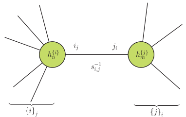
Figure 1: This figure illustrates our conventions on labelling external and internal lines in the case of two vertices.

Below we will use a slightly modified version of (52)

$$\big{(}{\cal J}^{\{i\}}-{\cal H}^{\{i\}}\frac{\partial}{\partial\bar{q}_{i_{j}}}\big{)}(\sum_{\{i\}}q^{\perp}_{i})\propto(\sum_{\{i\}}q^{\perp}_{i})$$ (67)

as well as

$$({\cal J}^{\{i\}}+{\cal J}^{\{j\}})(q_{i_{j}}^{\perp}+q_{j_{i}}^{\perp})\propto(q_{i_{j}}^{\perp}+q_{j_{i}}^{\perp}).$$ (68)

Finally, we introduce a notation for $q^{\perp}_{i_{j}}$ when it is expressed in terms of external momenta

$$Q^{\perp}_{i}\equiv-\sum_{\{i\}_{j}}q^{\perp}_{i},\qquad Q^{\perp}_{i,j}=\frac{1}{2}(Q^{\perp}_{i}-Q^{\perp}_{j}).$$ (69)

3.3 Single exchanges

First we note that

$$\frac{1}{2}({\cal H}^{\{i\}}-{\cal H}^{\{j\}})\big{(}\frac{\partial}{\partial\bar{q}_{i_{j}}}-\frac{\partial}{\partial\bar{q}_{j_{i}}}\big{)}h_{n}^{\{i\}}(q^{\perp}_{i_{j}})h_{m}^{\{j\}}(q^{\perp}_{j_{i}})$$

$$\qquad\qquad\qquad\qquad=\big{(}{\cal H}^{\{i\}}\frac{\partial}{\partial\bar{q}_{i_{j}}}+{\cal H}^{\{j\}}\frac{\partial}{\partial\bar{q}_{j_{i}}}\big{)}h_{n}^{\{i\}}\big{(}\tfrac{1}{2}(q^{\perp}_{i_{j}}-q^{\perp}_{j_{i}})\big{)}h_{m}^{\{j\}}\big{(}\tfrac{1}{2}(q^{\perp}_{j_{i}}-q^{\perp}_{i_{j}})\big{)},$$ (70)

where the arguments $q^{\perp}_{i_{j}}$ and $q^{\perp}_{j_{i}}$ should be replaced before evaluating derivatives as indicated. Then the right hand side of (61) can be written as

$$[H^{n},J^{m}]+[H^{m},J^{n}]$$

$$\;\;=\frac{1}{(n-1)!}\frac{1}{(m-1)!}\frac{1}{s_{i,j}}\big{(}-{\cal H}^{\{i\}}\frac{\partial}{\partial\bar{q}_{i_{j}}}-{\cal H}^{\{j\}}\frac{\partial}{\partial\bar{q}_{j_{i}}}\big{)}h_{n}^{\{i\}}\big{(}\tfrac{1}{2}(q^{\perp}_{i_{j}}-q^{\perp}_{j_{i}})\big{)}h_{m}^{\{j\}}\big{(}\tfrac{1}{2}(q^{\perp}_{j_{i}}-q^{\perp}_{i_{j}})\big{)},$$ (71)

where $s_{i,j}$ was defined in (66).

Next we proceed by adding and subtracting ${\cal J}^{\{i\}}+{\cal J}^{\{j\}}$, so as to produce operators that commute with the total momentum as in (67)

$$[H_{n},J_{m}]+[H_{m},J_{n}]$$

$$\qquad=\frac{1}{(n-1)!}\frac{1}{(m-1)!}\frac{1}{s_{i,j}}\big{(}{\cal J}^{\{i\}}+{\cal J}^{\{j\}}-{\cal H}^{\{i\}}\frac{\partial}{\partial\bar{q}_{i_{j}}}-{\cal H}^{\{j\}}\frac{\partial}{\partial\bar{q}_{j_{i}}}\big{)}$$

$$\qquad\qquad\qquad\qquad\qquad\qquad\qquad\qquad\qquad\;h_{n}^{\{i\}}\big{(}\tfrac{1}{2}(q^{\perp}_{i_{j}}-q^{\perp}_{j_{i}})\big{)}h_{m}^{\{j\}}\big{(}\tfrac{1}{2}(q^{\perp}_{j_{i}}-q^{\perp}_{i_{j}})\big{)}$$

$$\qquad-\frac{1}{(n-1)!}\frac{1}{(m-1)!}\frac{1}{s_{i,j}}\big{(}{\cal J}^{\{i\}}+{\cal J}^{\{j\}}\big{)}h_{n}^{\{i\}}\big{(}\tfrac{1}{2}(q^{\perp}_{i_{j}}-q^{\perp}_{j_{i}})\big{)}h_{m}^{\{j\}}\big{(}\tfrac{1}{2}(q^{\perp}_{j_{i}}-q^{\perp}_{i_{j}})\big{)}.$$ (72)

The operator that appears in the first term permits us to use momentum conservation inside $h_{m}$ and $h_{n}$, so we can eliminate $q^{\perp}_{i_{j}}$ and $q^{\perp}_{j_{i}}$ in favour of external momenta. After that $h_{n}$ and $h_{m}$ no longer depend on exchanged momenta explicitly, hence differential operators acting on them can be dropped. As a result, for the first term in (72) we obtain

$$\frac{1}{(n-1)!}\frac{1}{(m-1)!}\frac{1}{s_{i,j}}\big{(}{\cal J}^{\{i\}}+{\cal J}^{\{j\}}-{\cal H}^{\{i\}}\frac{\partial}{\partial\bar{q}_{i_{j}}}-{\cal H}^{\{j\}}\frac{\partial}{\partial\bar{q}_{j_{i}}}\big{)}$$

$$\qquad\qquad\qquad\qquad\qquad\qquad\qquad\qquad\qquad h_{n}^{\{i\}}\big{(}\tfrac{1}{2}(q^{\perp}_{i_{j}}-q^{\perp}_{j_{i}})\big{)}h_{m}^{\{j\}}\big{(}\tfrac{1}{2}(q^{\perp}_{j_{i}}-q^{\perp}_{i_{j}})\big{)}$$

$$\qquad\qquad\qquad\qquad\qquad\qquad\quad=\frac{1}{(n-1)!}\frac{1}{(m-1)!}\frac{1}{s_{i,j}}{\cal J}^{\{i-j\}}h_{n}^{\{i\}}(Q^{\perp}_{i,j})h_{m}^{\{j\}}(Q^{\perp}_{j,i}),$$ (73)

where $\{i-j\}$ and $Q^{\perp}_{i,j}$ were defined in (63) and (69).

Employing (68), the second term reads

$$-\frac{1}{(n-1)!}\frac{1}{(m-1)!}\frac{1}{s_{i,j}}\big{(}{\cal J}^{\{i\}}+{\cal J}^{\{j\}}\big{)}h_{n}^{\{i\}}\big{(}\tfrac{1}{2}(q^{\perp}_{i_{j}}-q^{\perp}_{j_{i}})\big{)}h_{m}^{\{j\}}\big{(}\tfrac{1}{2}(q^{\perp}_{j_{i}}-q^{\perp}_{i_{j}})\big{)}$$

$$\qquad\qquad\qquad\qquad\qquad=-\frac{1}{(n-1)!}\frac{1}{(m-1)!}\frac{1}{s_{i,j}}\big{(}{\cal J}^{\{i\}}+{\cal J}^{\{j\}}\big{)}h_{n}^{\{i\}}(q^{\perp}_{i_{j}})h_{m}^{\{j\}}(q^{\perp}_{j_{i}}).$$ (74)

Combining both contributions, we find that

$$[H_{n},J_{m}]+[H_{m},J_{n}] =\frac{1}{(n-1)!}\frac{1}{(m-1)!}\frac{1}{s_{i,j}}{\cal J}^{\{i-j\}}h_{n}^{\{i\}}(Q^{\perp}_{i,j})h_{m}^{\{j\}}(Q^{\perp}_{j,i})$$

$$-\frac{1}{(n-1)!}\frac{1}{(m-1)!}\frac{1}{s_{i,j}}\big{(}{\cal J}^{\{i\}}+{\cal J}^{\{j\}}\big{)}h_{n}^{\{i\}}(q^{\perp}_{i_{j}})h_{m}^{\{j\}}(q^{\perp}_{j_{i}}).$$ (75)

To interpret this result, first note that in the first term ${\cal J}^{\{i-j\}}$ acts only on external momenta. Let us denote it just by ${\cal J}$. In Section 4 it will be shown that $s_{i,j}$ commutes with ${\cal J}$. Using these facts one can rewrite the consistency condition (58) as

$$\sum_{k=0}^{n-2}[H_{n-k},J_{k+2}]={\cal J}\Big{(}\frac{1}{n!}h_{n}^{\{i\}}+\sum_{k=1}^{n-3}\frac{1}{(n-k-1)!}\frac{1}{(k+1)!}h^{\{i\}}_{n-k}(Q^{\perp}_{i,j})\frac{1}{s_{i,j}}h_{k+2}^{\{j\}}(Q^{\perp}_{j,i})\Big{)}$$

$$\qquad\qquad\qquad-\sum_{k=1}^{n-3}\frac{1}{(n-k-1)!}\frac{1}{(k+1)!}\frac{1}{s_{i,j}}\big{(}{\cal J}^{\{i\}}+{\cal J}^{\{j\}}\big{)}h_{n-k}^{\{i\}}(q^{\perp}_{i_{j}})h_{k+2}^{\{j\}}(q^{\perp}_{j_{i}})=0.$$ (76)

After multiplying the first line by $n!$ in brackets we recover the sum of the contact $n$-point diagram and of all exchanges involving $n$ external particles and a single propagator. The combinatorial factors

$$\frac{n!}{(n-k-1)!(k+1)!},$$ (77)

that appear in front of exchanges count all possible channels that each given exchange can have. As it was noted below (60), for $n-k=k+2$ the exchange will get an extra factor of $1/2$, which is the standard symmetry factor associated with a symmetry that interchanges identical vertices.

In other words, up to contributions from diagrams involving more than one propagator, the consistency condition (76) looks exactly as the Ward identity for the $n$-point amplitude, where ${\cal J}$ is the operator that verifies gauge invariance. At this point the term Ward identity may sound misleading, because in the light-cone approach gauge invariance is completely fixed. We will justify this terminology in Section 5, where we will make a connection between the light-cone approach and the spinor-helicity formalism.

3.4 Double exchanges

The second term on the right hand side of (75) is responsible for contributions of multiple exchanges to the Ward identity. To prevent possible confusions, let us clarify, that by double and multiple exchanges we mean tree-level diagrams that involve two or more internal lines.

In this Section we will show how to reproduce contributions from diagrams with two exchanges. To this end, let us focus on a particular diagram, which consists of two vertices $h^{\{k\}}_{p}$ and $h^{\{j\}}_{m}$ connected by a pair of exchanges and a vertex $h^{\{l\}}_{q}$, see Figure 2. The remaining contributions will be omitted, which will be indicated by $\to$ instead of $=$. To have the same number of external fields as in (75) we have to demand $p+q-2=n$. One finds

$$[H_{n},J_{m}]+[H_{m},J_{n}]\to-\frac{1}{(n-1)!}\frac{1}{(m-1)!}\frac{1}{s_{i,j}}{\cal J}^{\{i\}}h_{n}^{\{i\}}(q^{\perp}_{i_{j}})h_{m}^{\{j\}}(q^{\perp}_{j_{i}})$$

$$\to\frac{1}{(p-1)!}\frac{1}{(q-1)!}\frac{n}{(m-1)!}\frac{1}{s_{kl,j}}\frac{1}{\beta_{k_{l}}-\beta_{l_{k}}}h^{\{j\}}_{m}(q^{\perp}_{j_{i}})\big{(}\frac{\partial}{\partial\bar{q}_{k_{l}}}-\frac{\partial}{\partial\bar{q}_{l_{k}}}\big{)}h^{\{k\}}_{p}(q^{\perp}_{k_{l}})h^{\{l\}}_{q}(q^{\perp}_{l_{k}}).$$ (78)

To obtain the last line we used the consistency condition that relates $h_{n}^{\{i\}}$ to commutators involving the Hamiltonians of lower degrees $h^{\{k\}}_{p}$ and $h^{\{l\}}_{q}$. We also renamed $s_{i,j}\to s_{kl,j}$ to be consistent with the fact that the legs of the diagram, that before using the consistency condition for $h_{n}^{\{i\}}$ were labelled by $\{i\}$, after that belong to $h^{\{k\}}_{p}$ and $h^{\{l\}}_{q}$ and hence are labelled by the sets $\{k\}$ and $\{l\}$.

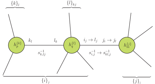
Figure 2: This figure illustrates how after using the consistency condition for $h_{n}^{\{i\}}$ its external lines previously labelled by $\{i\}_{j}$ split into two groups labelled by $\{k\}_{l}$ and $\{l\}_{kj}$. Accordingly, we rename $i_{j}\to l_{j}$, $j_{i}\to j_{l}$ and $s_{i,j}\to s_{kl,j}$.

We would like to remind the reader, that in the first line of (78) there is an implicit delta-function $\delta(q^{\perp}_{i_{j}}+q^{\perp}_{j_{i}})$, which relates momenta on different sides of the exchange. When we go to the second line, the set $\{i\}$ is split into $\{k\}$ and $\{l\}$ and the special index $i_{j}$ of the set $\{i\}$ can either belong to $\{k\}$ or to $\{l\}$. Here we keep only the terms, relevant to $\{k-l-j\}$ exchange that is those with $i_{j}\in\{l\}$. This produces an extra combinatorial factor $(q-1)/n$. As a result

$$[H_{n},J_{m}]+[H_{m},J_{n}]$$

$$\to\frac{1}{(p-1)!}\frac{1}{(q-2)!}\frac{1}{(m-1)!}\frac{1}{s_{kl,j}}\frac{1}{\beta_{k_{l}}-\beta_{l_{k}}}\big{(}\frac{\partial}{\partial\bar{q}_{k_{l}}}-\frac{\partial}{\partial\bar{q}_{l_{k}}}\big{)}h^{\{k\}}_{p}(q^{\perp}_{k_{l}})h^{\{l\}}_{q}(q^{\perp}_{l_{k}},q^{\perp}_{l_{j}})h^{\{j\}}_{m}(q^{\perp}_{j_{l}}),$$ (79)

where we also relabelled $i_{j}$ to $l_{j}$ and $j_{i}$ to $j_{l}$.

Leaving aside the combinatorial factor for a moment, we proceed with the rest analogously to a single exchange case

$$W^{\{k\text{-}l\text{-}j\}}_{1} \,\equiv\frac{1}{s_{kl,j}}\frac{1}{\beta_{k_{l}}-\beta_{l_{k}}}\big{(}\frac{\partial}{\partial\bar{q}_{k_{l}}}-\frac{\partial}{\partial\bar{q}_{l_{k}}}\big{)}h^{\{k\}}_{p}(q^{\perp}_{k_{l}})h^{\{l\}}_{q}(q^{\perp}_{l_{k}},q^{\perp}_{l_{j}})h^{\{j\}}_{m}(q^{\perp}_{j_{l}})$$

$$\,=-\frac{1}{s_{kl,j}}\frac{1}{s_{k,lj}}({\cal H}^{\{k\}}-{\cal H}^{\{l\}}-{\cal H}^{\{j\}})\big{(}\frac{\partial}{\partial\bar{q}_{k_{l}}}-\frac{\partial}{\partial\bar{q}_{l_{k}}}\big{)}h^{\{k\}}_{p}(q^{\perp}_{k_{l}})h^{\{l\}}_{q}(q^{\perp}_{l_{k}},q^{\perp}_{l_{j}})h^{\{j\}}_{m}(q^{\perp}_{j_{l}})$$

$$\,=-\frac{1}{s_{kl,j}}\frac{1}{s_{k,lj}}\big{(}{\cal H}^{\{k\}}\frac{\partial}{\partial\bar{q}_{k_{l}}}+({\cal H}^{\{l\}}+{\cal H}^{\{j\}})\frac{\partial}{\partial\bar{q}_{l_{k}}}\big{)}h_{p}^{\{k\}}\big{(}\tfrac{1}{2}(q^{\perp}_{k_{l}}-q^{\perp}_{l_{k}})\big{)}$$

$$\,\qquad\qquad\qquad\qquad\qquad\quad h_{q}^{\{l\}}\big{(}\tfrac{1}{2}(q^{\perp}_{l_{k}}-q^{\perp}_{k_{l}}),\tfrac{1}{2}(q^{\perp}_{l_{j}}-q^{\perp}_{j_{l}})\big{)}h_{m}^{\{j\}}\big{(}\tfrac{1}{2}(q^{\perp}_{j_{l}}-q^{\perp}_{l_{j}})\big{)}.$$ (80)

In a similar way, from $[H_{p},J_{q+m-2}]+[H_{q+m-2},J_{p}]$ we find another contribution

$$W^{\{k\text{-}l\text{-}j\}}_{2} \,\equiv-\frac{1}{s_{kl,j}}\frac{1}{s_{k,lj}}\big{(}({\cal H}^{\{k\}}+{\cal H}^{\{l\}})\frac{\partial}{\partial\bar{q}_{l_{j}}}+{\cal H}^{\{j\}}\frac{\partial}{\partial\bar{q}_{j_{l}}}\big{)}h_{p}^{\{k\}}\big{(}\tfrac{1}{2}(q^{\perp}_{k_{l}}-q^{\perp}_{l_{k}})\big{)}$$

$$\,\qquad\qquad\qquad\qquad\qquad\quad h_{q}^{\{l\}}\big{(}\tfrac{1}{2}(q^{\perp}_{l_{k}}-q^{\perp}_{k_{l}}),\tfrac{1}{2}(q^{\perp}_{l_{j}}-q^{\perp}_{j_{l}})\big{)}h_{m}^{\{j\}}\big{(}\tfrac{1}{2}(q^{\perp}_{j_{l}}-q^{\perp}_{l_{j}})\big{)}.$$ (81)

For the sum of two terms we proceed as for the single exchange case in (72): we add and subtract ${\cal J}^{\{k\}}+{\cal J}^{\{l\}}+{\cal J}^{\{j\}}$ producing an operator that allows to use momentum conservation inside the diagram. Namely,

$$W^{\{k\text{-}l\text{-}j\}}_{1} +W^{\{k\text{-}l\text{-}j\}}_{2}=\frac{1}{s_{kl,j}}\frac{1}{s_{k,lj}}\big{(}{\cal J}^{\{k\}}+{\cal J}^{\{l\}}+{\cal J}^{\{j\}}$$

$$\qquad\qquad\qquad-{\cal H}^{\{k\}}\frac{\partial}{\partial\bar{q}_{k_{l}}}-({\cal H}^{\{l\}}+{\cal H}^{\{j\}})\frac{\partial}{\partial\bar{q}_{l_{k}}}-({\cal H}^{\{k\}}+{\cal H}^{\{l\}})\frac{\partial}{\partial\bar{q}_{l_{j}}}-{\cal H}^{\{j\}}\frac{\partial}{\partial\bar{q}_{j_{l}}}\big{)}$$

$$\quad\qquad\qquad\qquad h_{p}^{\{k\}}\big{(}\tfrac{1}{2}(q^{\perp}_{k_{l}}-q^{\perp}_{l_{k}})\big{)}h_{q}^{\{l\}}\big{(}\tfrac{1}{2}(q^{\perp}_{l_{k}}-q^{\perp}_{k_{l}}),\tfrac{1}{2}(q^{\perp}_{l_{j}}-q^{\perp}_{j_{l}})\big{)}h_{m}^{\{j\}}\big{(}\tfrac{1}{2}(q^{\perp}_{j_{l}}-q^{\perp}_{l_{j}})\big{)}$$

$$\qquad\qquad-\frac{1}{s_{kl,j}}\frac{1}{s_{k,lj}}\big{(}{\cal J}^{\{k\}}+{\cal J}^{\{l\}}+{\cal J}^{\{j\}}\big{)}h^{\{k\}}_{p}(q^{\perp}_{k_{l}})h^{\{l\}}_{q}(q^{\perp}_{l_{k}},q^{\perp}_{l_{j}})h^{\{j\}}_{m}(q^{\perp}_{j_{l}}).$$ (82)

Employing (67) and (68), it is not hard to see that the operator in the first term allows to use

$$\sum_{\{k\}}q^{\perp}_{k}=0,\quad\sum_{\{l\}_{j}}q^{\perp}_{l}+\sum_{\{j\}_{l}}q^{\perp}_{j}=0,$$

$$\sum_{\{j\}}q^{\perp}_{j}=0,\quad\sum_{\{l\}_{k}}q^{\perp}_{l}+\sum_{\{k\}_{l}}q^{\perp}_{k}=0.$$ (83)

These momentum conservation conditions permit us to eliminate $q^{\perp}_{k_{l}}$, $q^{\perp}_{l_{k}}$, $q^{\perp}_{l_{j}}$ and $q^{\perp}_{l_{j}}$ expressing them in terms of external momenta. After that vertices no longer depend on exchanged momenta, so differential operators acting on them can be dropped. Thus, we find

$$W^{\{k\text{-}l\text{-}j\}}_{1}+W^{\{k\text{-}l\text{-}j\}}_{2} =\frac{1}{s_{kl,j}}\frac{1}{s_{k,lj}}{\cal J}^{\{k-l-j\}}h_{p}^{\{k\}}(Q^{\perp}_{k,lj})h_{q}^{\{l\}}(Q^{\perp}_{lj,k},Q^{\perp}_{kl,j})h_{m}^{\{j\}}(Q^{\perp}_{j,kl})$$

$$-\frac{1}{s_{kl,j}}\frac{1}{s_{k,lj}}\big{(}{\cal J}^{\{k\}}+{\cal J}^{\{l\}}+{\cal J}^{\{j\}}\big{)}h^{\{k\}}_{p}(q^{\perp}_{k_{l}})h^{\{l\}}_{q}(q^{\perp}_{l_{k}},q^{\perp}_{l_{j}})h^{\{j\}}_{m}(q^{\perp}_{j_{l}}).$$ (84)

The second line is responsible for contributions of diagrams involving at least three propagators. Reinstating the combinatorial factor from (79), for the first line of (84) we find

$$[H_{n},J_{m}]+[H_{m},J_{n}]+[H_{p},J_{q+m-2}]+[H_{q+m-2},J_{p}]$$

$$\quad\to\frac{1}{(p-1)!}\frac{1}{(q-2)!}\frac{1}{(m-1)!}{\cal J}h_{p}^{\{k\}}(Q^{\perp}_{k,lj})\frac{1}{s_{kl,j}}h_{q}^{\{l\}}(Q^{\perp}_{lj,k},Q^{\perp}_{kl,j})\frac{1}{s_{k,lj}}h_{m}^{\{j\}}(Q^{\perp}_{j,kl}).$$ (85)

This gives one of the double exchange contributions to the Ward identity involving a contact vertex of degree ${p+q+m-4}$. This contact vertex in our conventions goes with a prefactor $1/(p+q+m-4)!$. Normalising the contribution of the contact diagram to unity, we find that the double exchange from (85) appears with a factor

$$\frac{(p+q+m-4)!}{(p-1)!(q-2)!(m-1)!},$$ (86)

which just gives the total number of channels. This is exactly what we should expect from the Feynman rules if we symmetrise them over external fields, as in our approach.

3.5 General case

In the previous two Sections we showed that the consistency condition for the non-linear deformation in the light-cone approach (43) can be rewritten as the Ward identity involving contributions from contact diagrams, single exchanges and some extra terms bilinear in vertices of degrees lower than that of a contact contribution (76). Employing the consistency condition for these extra terms, they were shown to produce contributions of double exchanges plus extra terms, trilinear in vertices of yet lower degrees (84). This procedure should be repeated recursively until it terminates due to ${\cal J}h_{3}=0$, see (58), thus reproducing the Ward identity for the complete amplitude. The equation $[H,\bar{J}]=0$ is analogous. The results of this recursive procedure can be summarised as

Proposition 1.

The light-cone consistency condition can be equivalently rewritten as a set of Ward identities for all $n$-point amplitudes

$${\cal J}^{\{i\}}{\cal A}_{n}(q^{\perp}_{i})=0,\qquad\bar{\cal J}^{\{i\}}{\cal A}_{n}(q^{\perp}_{i})=0,$$ (87)

where

$${\cal J}^{\{i\}} \,=\sum_{i=1}^{n}\Big{(}-\frac{q_{i}\bar{q}_{i}}{\beta_{i}}\frac{\partial}{\partial\bar{q}_{i}}-q_{i}\frac{\partial}{\partial\beta_{i}}+\lambda_{i}\frac{q_{i}}{\beta_{i}}\Big{)},$$

$$\bar{\cal J}^{\{i\}} \,=\sum_{i=1}^{n}\Big{(}-\frac{q_{i}\bar{q}_{i}}{\beta_{i}}\frac{\partial}{\partial q_{i}}-\bar{q}_{i}\frac{\partial}{\partial\beta_{i}}+\lambda_{i}\frac{\bar{q}_{i}}{\beta_{i}}\Big{)}$$ (88)

and ${\cal A}_{n}(q^{\perp}_{i})$ is the off-shell light-cone amplitude constructed according to the following Feynman rules:

• the propagator, splitting the external fields into sets labelled by $\{k\}_{l}$ and $\{l\}_{k}$, is given by

  $$\frac{1}{s_{k,l}}=-\frac{2}{(\beta_{k_{l}}-\beta_{l_{k}})({\cal H}^{\{k\}}-{\cal H}^{\{l\}})},$$ (89)

  where

  $$\beta_{k_{l}}=-\sum_{\{k\}_{l}}\beta_{k}, \qquad{\cal H}^{\{k\}}=\sum_{\{k\}_{l}}h_{2}(q_{k}^{\perp})+h_{2}\big{(}-\sum_{\{k\}_{l}}q_{k}^{\perp}\big{)}$$

  $$\beta_{l_{k}}=-\sum_{\{l\}_{k}}\beta_{l}, \qquad{\cal H}^{\{l\}}=\sum_{\{l\}_{k}}h_{2}(q_{l}^{\perp})+h_{2}\big{(}-\sum_{\{l\}_{k}}q_{l}^{\perp}\big{)}.$$ (90)

  More explanations on our conventions are given in Section 3.2.

• Inside vertices, the momenta of exchanged fields $q_{k_{l}}^{\perp}$ and $q_{l_{k}}^{\perp}$ should be expressed in terms of momenta of external fields as

  $$q^{\perp}_{k_{l}}\to Q_{k,l}=\frac{1}{2}(-\sum_{\{k\}_{l}}q^{\perp}_{k}+\sum_{\{l\}_{k}}q^{\perp}_{l}),$$

  $$q^{\perp}_{l_{k}}\to Q_{l,k}=\frac{1}{2}(-\sum_{\{l\}_{k}}q^{\perp}_{l}+\sum_{\{k\}_{l}}q^{\perp}_{k}).$$ (91)

Alternatively, (87) can be written as

$$[A,J_{2}]=0,\qquad[A,\bar{J}_{2}]=0,$$ (92)

where $A$ is made of the amplitude ${\cal A}(q^{\perp})$ by contracting it with fields.

Let us now make several comments. First, as it was noted above, the amplitude ${\cal A}(q^{\perp})$ is an off-shell object. Indeed, in the light-cone approach neither the free Hamiltonian nor interaction terms depend on $q_{i}^{-}$. For this simple reason ${\cal A}(q^{\perp})$ defined above makes perfect sense for any $q_{i}^{-}$, not only for on-shell values $q_{i}^{-}\approx h_{2}(q_{i}^{\perp})$. Moreover, ${\cal A}({q^{\perp}})$ is related unambiguously to the Hamiltonian, so it defines the action.

It is worth to note the unusual form of the propagator (89), which we employed to construct ${\cal A}(q^{\perp})$. It follows from (64) that this propagator coincides with the one that comes from the covariant Feynman rules when external particles are on-shell. They are, nevertheless, different for off-shell external momental. This difference can be explained by the fact that the framework we are dealing with is the light-cone Hamiltonian perturbation theory, which has some peculiar features, see e.g. Kogut:1969xa .

We recall that to derive (87) we fixed the freedom of integration by parts in interaction terms by (55). Of course, this condition should not be important for consistency. In particular, it should be possible to use conservation of the total momentum inside ${\cal A}_{n}(q^{\perp})$. The resulting amplitude will no longer be annihilated by ${\cal J}^{\{i\}}$, but, as it is not hard to see, will produce terms proportional to ${\cal H}^{\{i\}}$. Returning back to the consistency conditions in the original form (48), one can see that such extra terms are harmless, as they can be absorbed by the appropriate redefinition of $j_{n}$. Thus, one can reformulate Proposition 1 above in a form, where integration by parts is allowed, but (87) holds only up to terms proportional to ${\cal H}^{\{i\}}$. One can then use the freedom of integration by parts to simplify slightly the Feynman rules presented above. In particular, it is not necessary to express momenta of internal lines in a symmetric way in terms of external momenta on both sides of a given propagator as in (91).

Note, that for four external lines (87) was found in Metsaev:1991mt ; Metsaev:1991nb . More precisely, it was observed that one can solve the light-cone consistency condition at the four-point level by taking the quartic vertex to be minus the sum of exchanges. Our analysis gives a simple derivation of this fact and extends it to all orders.

Finally, let us point out that even though the form (87) of the consistency condition looks much more natural from the perturbative field theory perspective, it is sometimes instructive to keep in mind the original form of the consistency condition as well. In particular, it is clear from (58) that once cubic interactions are consistent by themselves, that is $[H_{3},J_{3}]=0$, then by setting all higher vertices to zero we obtain a consistent theory. At the same time, using the language of (87) this translates into the statement, that once we verified that cubic vertices result into consistent four-point exchanges, then all higher-point exchanges involving only cubic vertices are also consistent. The latter statement is not so easily seen only from (87). The origin of this non-trivial translation between the two languages is the iterative procedure that we needed to undertake to derive (87) from (58). It would be interesting to find more non-trivial examples of this phenomenon.

4 Solution of the Ward identity

Previous analysis emphasises the central role played by operators ${\cal J}$ and $\bar{\cal J}$. It was shown that consistency of the non-linear deformation implies that these operators annihilate the total amplitude. In this Section we find a general solution of these equations.

4.1 External scalars

To start we find a general solution of (87) in the case when all external fields are scalars. The first equation explicitly reads

$${\cal J}^{\{i\}}{\cal A}_{n}(q_{i}^{\perp})=0,\qquad{\cal J}^{\{i\}}=\sum_{i=1}^{n}\left(-\frac{q_{i}\bar{q}_{i}}{\beta_{i}}\frac{\partial}{\partial\bar{q}_{i}}-q_{i}\frac{\partial}{\partial\beta_{i}}\right).$$ (93)

We remind the reader that the Hamiltonian should satisfy kinematical constraints (38)-(41). By inspecting the Feynman rules given in the previous Section, it is not hard to see that the same kinematical constraints carry over to the total amplitude.

As it was mentioned above, the first two conditions (38), (39) imply that the amplitude is a general function of the following varaibles

$$\bar{\mathbb{P}}_{ij}\equiv\bar{q}_{i}\beta_{j}-\bar{q}_{j}\beta_{i},\qquad\mathbb{P}_{ij}\equiv q_{i}\beta_{j}-q_{j}\beta_{i},\qquad\beta_{i}.$$ (94)

This can be seen, for instance, by considering characteristic vector fields associated with differential equations (38), (39). Variables (94) provide an overcomplete set of invariants of the associated characteristic flows.

When we add an extra differential equation (93), clearly, the set of invariants can only be reduced. Upon proper dressing with $\beta$ dependence, both $\bar{\mathbb{P}}_{ij}$ and $\mathbb{P}_{ij}$ can be promoted to solutions of (93)

$$\bar{\mathbb{P}}_{ij}\to\bar{\Pi}_{ij}\equiv\frac{\bar{\mathbb{P}}_{ij}}{\beta_{i}\beta_{j}}:\qquad\qquad{\cal J}^{\{i\}}\bar{\Pi}_{ij}=0,\qquad{\cal J}^{\{i\}}\mathbb{P}_{ij}=0.$$ (95)

It is not hard to see that there are no solutions of (93) that depend on $\beta_{i}$ alone, so ${\cal A}_{n}(q_{i}^{\perp})$ is an arbitrary function of $\bar{\Pi}_{ij}$ and $\mathbb{P}_{ij}$. It is convenient to phrase this conclusion as

$${\cal A}_{n}(q_{i}^{\perp})=\phi(\bar{\mathbb{P}}_{ij},\mathbb{P}_{ij},\beta_{i}),\qquad-N_{\beta_{i}}=N_{\langle i|},$$ (96)

where

$$N_{\langle i|}\equiv\sum_{j=1}^{n}N_{\mathbb{P}_{ij}}$$ (97)

counts the total homogeneity degree of all $\mathbb{P}_{ij}$’s with fixed $i$ and any $j$.

Similarly, to solve

$$\bar{\cal J}^{\{i\}}{\cal A}_{n}(q_{i}^{\perp})=0,\qquad\bar{\cal J}^{\{i\}}=\sum_{i=1}^{n}\left(-\frac{q_{i}\bar{q}_{i}}{\beta_{i}}\frac{\partial}{\partial q_{i}}-\bar{q}_{i}\frac{\partial}{\partial\beta_{i}}\right)$$ (98)

we introduce new variables $\Pi_{ij}$

$${\mathbb{P}}_{ij}\to\Pi_{ij}\equiv\frac{{\mathbb{P}}_{ij}}{\beta_{i}\beta_{j}}:\qquad\qquad\bar{\cal J}^{\{i\}}\bar{\mathbb{P}}_{ij}=0,\qquad\bar{\cal J}^{\{i\}}\Pi_{ij}=0$$ (99)

and find that ${\cal A}_{n}(q_{i}^{\perp})$ is some function of $\bar{\mathbb{P}}_{ij}$ and $\Pi_{ij}$, which is equivalent to

$${\cal A}_{n}(q_{i}^{\perp})=\phi(\bar{\mathbb{P}}_{ij},\mathbb{P}_{ij},\beta_{i}),\qquad-N_{\beta_{i}}=N_{|i]},$$ (100)

where

$$N_{|i]}\equiv\sum_{j=1}^{n}N_{\bar{\mathbb{P}}_{ij}}$$ (101)

counts the total homogeneity degree of all $\bar{\mathbb{P}}_{ij}$’s with fixed $i$ and any $j$.

Combining (96) and (100) we find that

$$N_{|i]}=N_{\langle i|}.$$ (102)

Provided (102) is satisfied, we can rewrite the remaining homogeneity constraint as

$$-N_{\beta_{i}}=\frac{N_{|i]}+N_{\langle i|}}{2}.$$ (103)

It can be solved as

$${\cal A}_{n}(q_{i}^{\perp})=\chi([ij],\langle ij\rangle),$$ (104)

where

$$[ij]\equiv\frac{\sqrt{2}}{\sqrt{\beta_{i}\beta_{j}}}\bar{\mathbb{P}}_{ij},\qquad\langle ij\rangle\equiv-\frac{\sqrt{2}}{\sqrt{\beta_{i}\beta_{j}}}\mathbb{P}_{ij}.$$ (105)

Here the numerical coefficients have been chosen so as to agree with the standard conventions of the spinor-helicity approach reviewed in Appendix A.

In the next Section it will be used that $[ij]$ and $\langle ij\rangle$ can be factorised in terms of helicity spinors

$$|i]_{a}=\frac{2^{\frac{1}{4}}}{\sqrt{\beta_{i}}}\left(\begin{array}[]{c}\bar{q}_{i}\\ -\beta_{i}\end{array}\right),\qquad\langle i|_{\dot{b}}=\frac{2^{\frac{1}{4}}}{\sqrt{\beta_{i}}}\left(\begin{array}[]{ccc}q_{i}&&-\beta_{i}\end{array}\right)$$ (106)

as

$$[ij] \,=\varepsilon^{ab}|j]_{a}|i]_{b}=\frac{2^{\frac{1}{4}}}{\sqrt{\beta_{j}}}\left(\begin{array}[]{ccc}\bar{q}_{j}&&-\beta_{j}\end{array}\right)\left(\begin{array}[]{ccc}0&&1\\ -1&&0\end{array}\right)\frac{2^{\frac{1}{4}}}{\sqrt{\beta_{i}}}\left(\begin{array}[]{c}\bar{q}_{i}\\ -\beta_{i}\end{array}\right),$$ (112)

$$\langle ij\rangle \,=\varepsilon^{\dot{a}\dot{b}}\langle i|_{\dot{a}}\langle j|_{\dot{b}}=\frac{2^{\frac{1}{4}}}{\sqrt{\beta_{i}}}\left(\begin{array}[]{ccc}q_{i}&&-\beta_{i}\end{array}\right)\left(\begin{array}[]{ccc}0&&1\\ -1&&0\end{array}\right)\frac{2^{\frac{1}{4}}}{\sqrt{\beta_{j}}}\left(\begin{array}[]{c}q_{j}\\ -\beta_{j}\end{array}\right).$$ (118)

In these terms (102) reads

$$N_{|i]}-N_{\langle i|}=0,\qquad N_{|i]}=|i]\frac{\partial}{\partial|i]},\qquad N_{\langle i|}=\langle i|\frac{\partial}{\partial\langle i|}.$$ (119)

Equation (104) supplemented with a homogeneity constraint (119) gives a general solution of the Ward identities (93), (98) in the case of external scalars.

4.2 General case

In this Section we prove

Proposition 2.

A general solution of the Ward identities

$${\cal J}^{\{i\}}{\cal A}_{n}(q_{i}^{\perp}) \,=0,\qquad{\cal J}^{\{i\}}=\sum_{i=1}^{n}\left(-\frac{q_{i}\bar{q}_{i}}{\beta_{i}}\frac{\partial}{\partial\bar{q}_{i}}-q_{i}\frac{\partial}{\partial\beta_{i}}+\lambda_{i}\frac{q_{i}}{\beta_{i}}\right),$$

$$\bar{\cal J}^{\{i\}}{\cal A}_{n}(q_{i}^{\perp}) \,=0,\qquad\bar{\cal J}^{\{i\}}=\sum_{i=1}^{n}\left(-\frac{q_{i}\bar{q}_{i}}{\beta_{i}}\frac{\partial}{\partial q_{i}}-\bar{q}_{i}\frac{\partial}{\partial\beta_{i}}-\lambda_{i}\frac{\bar{q}_{i}}{\beta_{i}}\right)$$ (120)

is given by

$${\cal A}_{n}(q_{i}^{\perp})=\chi([ij],\langle ij\rangle),$$ (121)

where $\chi$ satisfies a homogeneity condition

$$(-N_{|i]}+N_{\langle i|}+2\lambda_{i})\chi([ij],\langle ij\rangle)=0$$ (122)

for every $i$. Spinor products are defined in (105).

To show this, let us first verify that (121), (122) is indeed a solution. To evaluate how the differential part of ${\cal J}^{\{i\}}$ acts on $\chi$ we use

$$-\sum_{i=1}^{n}\frac{q_{i}\bar{q}_{i}}{\beta_{i}}\frac{\partial}{\partial\bar{q}_{i}}|j] \,=-\sum_{i=1}^{n}\frac{q_{i}}{\beta_{i}}N_{\bar{q}_{i}}\frac{2^{\frac{1}{4}}}{\sqrt{\beta_{j}}}\left(\begin{array}[]{c}\bar{q}_{j}\\ -\beta_{j}\end{array}\right)=-\frac{q_{j}}{\beta_{j}}\left(\begin{array}[]{cccc}1&&&0\\ 0&&&0\end{array}\right)|j],$$ (127)

$$-\sum_{i=1}^{n}q_{i}\frac{\partial}{\partial\beta_{i}}|j] \,=-\sum_{i=1}^{n}\frac{q_{i}}{\beta_{i}}N_{\beta_{i}}\frac{2^{\frac{1}{4}}}{\sqrt{\beta_{j}}}\left(\begin{array}[]{c}\bar{q}_{j}\\ -\beta_{j}\end{array}\right)=\frac{1}{2}\frac{q_{j}}{\beta_{j}}\left(\begin{array}[]{ccc}1&&0\\ 0&&-1\end{array}\right)|j],$$ (132)

$$-\sum_{i=1}^{n}q_{i}\frac{\partial}{\partial\beta_{i}}\langle j| \,=-\sum_{i=1}^{n}\frac{q_{i}}{\beta_{i}}N_{\beta_{i}}\frac{2^{\frac{1}{4}}}{\sqrt{\beta_{j}}}\left(\begin{array}[]{ccc}q_{j}&&-\beta_{j}\end{array}\right)=\frac{1}{2}\frac{q_{j}}{\beta_{j}}\langle j|\left(\begin{array}[]{ccc}1&&0\\ 0&&-1\end{array}\right)$$ (136)

and the Leibniz rule. We find

$${\cal J}^{\{i\}}\chi([ij],\langle ij\rangle)= \,\sum_{i=1}^{n}\frac{q_{i}}{\beta_{i}}\Big{(}-\frac{1}{2}|i]\frac{\partial}{\partial|i]}+\frac{1}{2}\langle i|\left(\begin{array}[]{ccc}1&&0\\ 0&&-1\end{array}\right)\frac{\partial}{\partial\langle i|}+\lambda_{i}\Big{)}\chi([ij],\langle ij\rangle)$$ (139)

$$\qquad\qquad\qquad\qquad\qquad=-\sum_{i=1}^{n}\frac{q_{i}}{\beta_{i}}\langle i|\left(\begin{array}[]{cccc}0&&&0\\ 0&&&1\end{array}\right)\frac{\partial}{\partial\langle i|}\chi([ij],\langle ij\rangle),$$ (142)

where to get to the last line we used the homogeneity condition (122). Now we take into account that in $\chi$ spinors can only appear in the form of spinor contractions

$${\cal J}^{\{i\}}\chi([ij],\langle ij\rangle)=-\sum_{i,k,l=1}^{n}\frac{q_{i}}{\beta_{i}}\langle i|\left(\begin{array}[]{cccc}0&&&0\\ 0&&&1\end{array}\right)\frac{\partial\langle kl\rangle}{\partial\langle i|}\frac{\partial}{\partial\langle kl\rangle}\chi([ij],\langle ij\rangle).$$ (143)

Using that

$$-\sum_{i=1}^{n}\frac{q_{i}}{\beta_{i}}\langle i|\left(\begin{array}[]{cccc}0&&&0\\ 0&&&1\end{array}\right)\frac{\partial}{\partial\langle i|}\langle kl\rangle=-\frac{q_{k}}{\beta_{k}}\frac{\sqrt{2}}{\sqrt{\beta_{k}\beta_{l}}}\left(\begin{array}[]{ccc}q_{k}&&-\beta_{k}\end{array}\right)\left(\begin{array}[]{cccc}0&&&0\\ 0&&&1\end{array}\right)\left(\begin{array}[]{ccc}0&&1\\ -1&&0\end{array}\right)\left(\begin{array}[]{c}q_{l}\\ -\beta_{l}\end{array}\right)$$ (153)

$$\qquad\qquad\qquad\qquad\qquad+\frac{q_{l}}{\beta_{l}}\frac{\sqrt{2}}{\sqrt{\beta_{k}\beta_{l}}}\left(\begin{array}[]{ccc}q_{l}&&-\beta_{l}\end{array}\right)\left(\begin{array}[]{cccc}0&&&0\\ 0&&&1\end{array}\right)\left(\begin{array}[]{ccc}0&&1\\ -1&&0\end{array}\right)\left(\begin{array}[]{c}q_{k}\\ -\beta_{k}\end{array}\right)=0,$$ (161)

we find

$${\cal J}^{\{i\}}\chi([ij],\langle ij\rangle)=0.$$ (162)

Analogously one can show that $\chi$ is annihilated by $\bar{\cal J}^{\{i\}}$, so we conclude that (121), (122) indeed solves (120).

Finally, let us assume that there is another solution $\chi^{\prime}$ of (120), which cannot be written in the form (121), (122). Then, as it is not hard to see, $\chi^{\prime}/\chi$ satisfies the scalar Ward identities (93), (98) and cannot be written in the form (104), (119). This contradicts the results of the previous Section, hence, $\chi^{\prime}$ does not exist.

In the four-point case the light-cone Ward identity (120) was solved previously in Metsaev:1991mt ; Metsaev:1991nb ; Bengtsson:2016hss . Our solution extends these result to any number of external points. Moreover, unlike previous results, solution (121), (122) is not limited to the class of polynomials in transverse momenta. This extension is, in fact, important, as the primary meaning of this solution is to give all possible consistent total amplitudes, which are typically non-local due to contributions from exchanges.

Back to the Mandelstam variables.

Now we can easily resolve a loose end left from Section 3 and prove that the Mandelstam variables can be pulled through ${\cal J}$ to form exchanges. The algebraic part of ${\cal J}$ clearly commutes with $s_{i,j}$, so it remains to prove that $s_{i,j}$ is annihilated by the differential part of ${\cal J}$.

It is straightforward to compute

$$(\sum_{\{i\}_{j}}\vec{q}_{i})^{2}=\sum_{k,l\in\{i\}_{j}}\vec{q}_{k}\cdot\vec{q}_{l}\approx\sum_{k,l\in\{i\}_{j}}\big{(}q_{k}\bar{q}_{l}+\bar{q}_{k}q_{l}-\frac{q_{k}\bar{q}_{k}}{\beta_{k}}\beta_{l}-\beta_{k}\frac{q_{l}\bar{q}_{l}}{\beta_{l}}\big{)}=\frac{1}{2}\sum_{k,l\in\{i\}_{j}}{[kl]\langle kl\rangle}.$$ (163)

Comparing this with (64)-(66) we find

$$s_{i}=\frac{1}{2}\sum_{k,l\in\{i\}_{j}}{[kl]\langle kl\rangle},\qquad s_{i,j}=\frac{1}{4}\sum_{k,l\in\{i\}_{j}}{[kl]\langle kl\rangle}+\frac{1}{4}\sum_{k,l\in\{j\}_{i}}{[kl]\langle kl\rangle}.$$ (164)

Note that these formulas hold off-shell. They imply that $s_{i,j}$ can be presented in the form (104), (119) and consequently commutes with ${\cal J}$, as it was argued. The same applies to $\bar{\cal J}$.

5 Interpretation

In preceding Sections we first found that the light-cone consistency condition can be rewritten in the form of the Ward identity for the amplitude, constructed form the light-cone Hamiltonian. Then we showed that a general solution of the Ward identity can be conveniently presented in terms of spinor products. These spinor products is a basic building block of the spinor-helicity approach, which is effectively used for computations of amplitudes in theories of massless particles. In particular, the spinor-helicity approach is to large extent responsible for the existence of extremely compact representations of tree and loop partial amplitudes in QCD. In this Section, we would like to draw a link between the outcome of our light-cone analysis and the spinor-helicity approach aiming to interpret the results we found, use the ideas from the spinor-helicity approach to plot a strategy for construction of massless higher-spin interactions and to see whether the light-cone analysis has something new to offer compared to the spinor-helicity approach. We start by briefly reviewing the spinor-helicity approach. Our review is not meant to be self-contained. We refer the reader to Dixon:1996wi ; Bern:2007dw ; Elvang:2013cua for general reviews and to Benincasa:2007xk ; Conde:2016izb for discussions more focused on the higher-spin case.

In four space-time dimension, any null vector can be represented as

$$q_{a\dot{b}}\equiv q_{\mu}(\sigma^{\mu})_{a\dot{b}}=\sqrt{2}\left(\begin{array}[]{ccc}q^{-}&&\bar{q}\\ q&&-q^{+}\end{array}\right)\approx\sqrt{2}\left(\begin{array}[]{ccc}-\frac{q\bar{q}}{\beta}&&\bar{q}\\ q&&-\beta\end{array}\right)=-|q]_{a}\langle q|_{\dot{b}},$$ (165)

where $|q]_{a}$ and $\langle q|_{\dot{b}}$ are simply on-shell Weyl spinors with momentum $q$

$$|q]_{a}=\frac{2^{\frac{1}{4}}}{\sqrt{\beta}}\left(\begin{array}[]{c}\bar{q}\\ -\beta\end{array}\right),\qquad\langle q|_{\dot{b}}=\frac{2^{\frac{1}{4}}}{\sqrt{\beta}}\left(\begin{array}[]{ccc}q&&-\beta\end{array}\right).$$ (166)

In the spinor-helicity approach representation (165) is used to define momenta of massless particles of any spin. We will use the standard notation $|i]\equiv|q_{i}]$ and $\langle i|\equiv\langle q_{i}|$. More conventions are given in Appendix A.

To encode polarisations one uses auxiliary massless vectors called reference momenta. For example, the polarisation vector $\epsilon^{\mu}_{1}(q;k)$ of a helicity one boson of momentum $q$ is defined as

$$\epsilon_{1}^{\mu}(q;k)=-\frac{\langle k|\gamma^{\mu}|q]}{\sqrt{2}\langle kq\rangle},$$ (167)

where $k$ is the reference momentum. It is easy to see that the polarisation vector defined above is transversal to $q$, that is $q_{\mu}\epsilon_{1}^{\mu}(q;k)=0$, as required by the Ward identity. The arbitrariness in the choice of the reference momentum is just a manifestation of gauge redundancy. For each external field one is free to choose a reference momentum independently. However, this choice should be consistent for all diagrams relevant to the process. Then, as a consequence of gauge invariance, auxiliary reference vectors drop out from the final answer. In other words, a consistent amplitude should be a function of spinor products $[ij]$ and $\langle ij\rangle$ only.

It is clear from (165) that $q_{\mu}$ is invariant with respect to the following scaling transformations

$$\langle q|\to t\langle q|,\qquad|q]\to t^{-1}|q].$$ (168)

For $|\lambda|=1$ this generates the action of the Wigner little group on the helicity spinors. If we compute amplitudes using the Feynman rules, then we can see that the only way this scaling contributes to the amplitude is through polarisation vectors. For a helicity one boson the polarisation vector (167) scales as

$$\epsilon_{1}^{\mu}(q;k)\to t^{-2}\epsilon_{1}^{\mu}(q;k).$$ (169)

More generally, the Wigner little group acts on the helicity-$\lambda$ polarisation vector as

$$\epsilon_{1}^{\mu}(q;k)\to t^{-2\lambda}\epsilon_{1}^{\mu}(q;k).$$ (170)

Each external field can be subjected to (168) independently. For an amplitude expressed in terms of spinor contractions to reproduce this scaling behaviour it should satisfy

$$(-N_{|i]}+N_{\langle i|}+2\lambda_{i}){\cal A}_{n}([jk],\langle jk\rangle)=0.$$ (171)

We find that despite a slightly different motivation, the spinor-helicity approach produces the same constraints that we found previously from the Poincare algebra closure in the light-cone deformation procedure. As we just reviewed, in the spinor-helicity approach the only two constraints are gauge invariance, which requires the amplitude to be expressed in terms of spinor products, and invariance with respect to the action of the Wigner little group, which fixes the homogeneity degrees of spinors. In the light-cone approach the only constraint is invariance with respect to the fully non-linear action of the Poincare algebra, which according to Proposition 1 can be replaced by invariance of the amplitude with respect to the linear action of the algebra generators. Solving these constraints, we indeed find that the light-cone amplitude can be expressed in terms of spinor products only, which through the spinor-helicity approach relates (120) to gauge invariance and, thus, justifies the term the Ward identity that we used. Moreover, (120) fixes the homogeneity degrees of spinors, which from the spinor-helicity perspective is related to the Wigner little group invariance. This relation can be easily seen from the light-cone approach itself. Namely, by acting along the lines of Section 4.2, one can show that $[{\cal A}_{n},J_{2}^{x\bar{x}}]=0$ implies (122).

So far we could see that on-shell amplitudes from the spinor-helicity approach appear to be very similar to light-cone amplitudes ${\cal A}_{n}(q^{\perp})$, which we introduced above. However, it is important to remember that ${\cal A}_{n}(q^{\perp})$ in the light-cone approach is well defined for off-shell momenta. In particular, ${\cal A}_{n}(q^{\perp})$ can be used to define the light-cone Hamiltonian and then the action via the Legendre transform. This difference originates from the way one defines spinors $|i]$ and $\langle i|$ in the two approaches. In the spinor-helicity approach spinors $|i]$ and $\langle i|$ are only defined for null momenta, that is for $q^{-}\approx h_{2}(q^{\perp})$, see (165), (166). In the light-cone approach one defines spinors by the very same formula (166), but the momentum is not required to be massless and $q^{-}$ can be arbitrary. Clearly, factorisation formula (165) does not work off-shell, but in the light-cone approach it is never used. It is quite remarkable that this rather trivial off-shell extension of spinor products and, hence, of the amplitude turns out to be consistent without any further constraints. This can be regarded as a simple consequence of $q^{-}$-independence of the Feynman rules presented in Proposition 1.

An immediate benefit from the off-shell extension of helicity spinors is that they can be used for momenta on internal lines. So, in the light-cone approach exchanges can also be written in terms of spinor products. More details on how they are constructed can be found in Proposition 1. Generically, when internal momenta are expressed in terms of momenta on external lines, exchanges cannot be written in terms of spinor products any more. This implies that they do not satisfy the Ward identity. Consequently, individual contact interactions, in general, violate the Ward identity either.

This suggests to reconsider the light-cone deformation procedure and focus on seeking the amplitude instead of the Hamiltonian. The benefit of this strategy is concisely summarised by (92): the amplitude satisfies a simple linear differential equation, while the equation for the Hamiltonian is quadratic in deformations. Having found a general solution for the amplitude we, thus, found a general solution of the light-cone deformation procedure. Note, however, that these solutions generically are associated with non-local Hamiltonians. The problem of finding consistent amplitudes that result in local Hamiltonians deserves a separate thorough analysis. Let us, nevertheless, make few comments on this point.

Locality.

Typically, in the light-cone approach one defines locality as a requirement that the Hamiltonian is polynomial in transverse momenta or, equivalently, in $\bar{\mathbb{P}}_{ij}$ and ${\mathbb{P}}_{kl}$. The same Hamiltonian can brought to many different forms using momentum conservation. Clearly, the Hamiltonian is local if there exist at least one of its forms where it is polynomial in transverse momenta. Due to the possibility to use momentum conservation locality may not be manifest. For example, the antiholomorphic part of the Yang-Mills cubic vertex can be written as

$$h_{3}=\frac{[12]^{3}}{[23][31]}=\sqrt{2}\frac{\bar{\mathbb{P}}^{3}_{12}\beta_{3}}{\bar{\mathbb{P}}_{23}\bar{\mathbb{P}}_{31}\beta_{1}\beta_{2}}.$$ (172)

This vertex is superficially non-local as it contains powers of transverse momenta in the denominator. However, it is easy to see that momentum conservation implies

$$\bar{\mathbb{P}}_{12}=\bar{\mathbb{P}}_{23}=\bar{\mathbb{P}}_{31},$$ (173)

hence, non-locality of (172) is spurious. This example illustrates that to make locality manifest it may be required to break the spinor-helicity representation. At the cubic level this subtlety does not result in any difficulties, because modulo momentum conservation there is only one possible Lorentz-invariant variable that depends on the antiholomorphic momentum (173) and, similarly, only one that depends on the holomorphic one. It would be interesting to clarify how this phenomenon extends to higher-point amplitudes.

Locality of the Hamiltonian is naturally translated into the language of amplitudes using the framework of on-shell methods Britto:2004ap ; Britto:2005fq . Namely, it is required that amplitudes have no other singularities than those produced by exchanges. In many cases one can also justify that amplitudes vanish in certain directions at complex infinity. This allows to reconstruct them unambiguously from their singularities. In this respect we would like to clarify that the light-cone deformation procedure alone does not impose any constraints on the behaviour of amplitudes at infinity. Let us also note that the solution (121), (122) is not limited to polynomials in transverse momenta, so it is applicable to amplitudes, which are typically non-local due to contributions from exchanges.

It is worth to remark separately that in higher-spin theories imposing locality as described above, most likely, would rule out any interactions at all. It is then suggestive to replace locality in a strict sense by a milder requirement that coefficients of higher derivative terms decrease fast enough, so that the amplitudes associated with contact interactions do not contain singularities. This weaker version of locality was discussed at length in Bekaert:2015tva . Let us also note that it is this weaker version of locality, that is effectively implemented by the on-shell methods, as they just require contact interactions to be free of singularities.

Finally, we remark that contrary to the way one usually defines locality for the light-cone deformation procedure, the on-shell methods require locality of interactions only on-shell. It would be interesting to clarify whether this difference can play any role.

6 Conclusion

This paper contains two main results. First, we show that the light-cone consistency conditions can be equivalently rephrased as a set of Ward identities for the light-cone off-shell amplitudes. Then we give a general solution to these Ward identities. This solution acquires an extremely simple form when written using the spinor-helicity language. More precisely, the general solution is just any function of spinor products that satisfies a well-known constraint relating homogeneity degrees of spinors with helicities of external fields. These results are summarised in Proposition 1 and Proposition 2.

Our primary goal is to employ the light-cone analysis to construct interactions of massless higher-spin fields. In this respect, our results provide a general solution to this problem in the case when locality of interactions is not required. Of course, this way of solving the consistent interaction problem is to large extent trivial, see, e.g., Barnich:1993vg . Nevertheless, this gives a good starting point to address the problem of local interactions.

To construct local interactions, it is suggestive to proceed in the spirit of the on-shell methods Britto:2004ap ; Britto:2005fq , that is by reconstructing amplitudes from singularities associated with exchanges. In other words, it seems more reasonable to seek not the individual vertices, but the total amplitude. Indeed, the total amplitude satisfies the Ward identities, which have been solved in the present paper in complete generality. At the same time, constraints on individual contact interactions are much more complicated and from particular examples we know that individual vertices can be quite cumbersome Ponomarev:2016lrm . More generally, amplitudes, being physically observable quantities, are much more constrained than individual vertices which are, moreover, prone to ambiguities of a gauge choice, field redefinitions, different sets of auxiliary fields etc. One should not expect a simple form of individual vertices unless these ambiguities are fixed wisely. On the contrary, as a result of strong constraints put on them, amplitudes admit a concise spinor-helicity representation.

Having written the light-cone consistency condition in the spinor-helicity form, we are able to clarify that the light-cone analysis does not impose any constraints on the behaviour of the amplitude at infinity. Hence, the no-go conclusions based on BCFW Benincasa:2007xk ; Fotopoulos:2010ay ; Benincasa:2011pg ; McGady:2013sga ; Ponomarev:2016jqk ; Bengtsson:2016alt , in principle, can be circumvented, see also Bengtsson:2016hss . Moreover, the explicit analysis of the quartic self-interaction sector Ponomarev:2016lrm shows that the relevant consistent interaction does exist.

It is worth to emphasise that the light-cone approach leads to a natural off-shell continuation of the spinor-helicity representation, which is usually defined on-shell. Once continued off-shell the light-cone amplitudes unambiguously define the action of the theory. It would be interesting to see whether the light-cone off-shell continuation can be used to promote on-shell results, such as colour-kinematics duality Bern:2008qj ; Bern:2010ue , to the off-shell level. Other interesting directions include extensions of the spinor-helicity approach to massive particles, as well as to AdS.

Appendix A Notations

Here we collected various notations used throughout the paper.

Light-cone coordinates.

We work with the 4d Minkowski space endowed with the mostly plus metric

$$ds^{2}=-(dx^{0})^{2}+(dx^{1})^{2}+(dx^{2})^{2}+(dx^{3})^{2}.$$ (174)

In the light-cone coordinates

$$x^{+} \,=\frac{1}{\sqrt{2}}(x^{3}+x^{0}), x^{-} \,=\frac{1}{\sqrt{2}}(x^{3}-x^{0}),$$

$$x \,=\frac{1}{\sqrt{2}}(x^{1}-ix^{2}), \bar{x} \,=\frac{1}{\sqrt{2}}(x^{1}+ix^{2}),$$ (175)

it becomes

$$ds^{2}=2dx^{+}dx^{-}+2dxd\bar{x}.$$ (176)

Accordingly, we denote

$$\partial^{-} \,=\frac{1}{\sqrt{2}}(\partial^{3}-\partial^{0}), \partial^{+} \,=\frac{1}{\sqrt{2}}(\partial^{3}+\partial^{0}),$$

$$\bar{\partial} \,=\frac{1}{\sqrt{2}}(\partial^{1}-i\partial^{2}), \partial \,=\frac{1}{\sqrt{2}}(\partial^{1}+i\partial^{2}),$$ (177)

which implies

$$\partial^{+}x^{-}=\partial^{-}x^{+}=\bar{\partial}x=\partial\bar{x}=1.$$ (178)

In the light-cone approach $x^{+}$ is taken to be the time variable and $\partial^{-}$ is the time derivative. Moreover, one assumes that $\partial^{+}$ is non-zero and can always be inverted.

Spinor-helicity.

For spinor-helicity conventions we follow Elvang:2013cua . We choose the Pauli matrices as

$$\sigma^{0}=\left(\begin{array}[]{cccc}1&&&0\\ 0&&&1\end{array}\right),\quad\sigma^{1}=\left(\begin{array}[]{cccc}0&&&1\\ 1&&&0\end{array}\right),\quad\sigma^{2}=\left(\begin{array}[]{ccc}0&&-i\\ i&&0\end{array}\right),\quad\sigma^{3}=\left(\begin{array}[]{ccc}1&&0\\ 0&&-1\end{array}\right).$$ (179)

Then

$$q_{a\dot{b}}\equiv q_{\mu}(\sigma^{\mu})_{a\dot{b}}=\sqrt{2}\left(\begin{array}[]{ccc}q^{-}&&\bar{q}\\ q&&-q^{+}\end{array}\right)\approx\sqrt{2}\left(\begin{array}[]{ccc}-\frac{q\bar{q}}{\beta}&&\bar{q}\\ q&&-\beta\end{array}\right)=-|q]_{a}\langle q|_{\dot{b}},$$ (180)

where

$$|q]_{a}=\frac{2^{\frac{1}{4}}}{\sqrt{\beta}}\left(\begin{array}[]{c}\bar{q}\\ -\beta\end{array}\right),\qquad\langle q|_{\dot{b}}=\frac{2^{\frac{1}{4}}}{\sqrt{\beta}}\left(\begin{array}[]{ccc}q&&-\beta\end{array}\right).$$ (181)

In these terms

$$[pq]=[p|^{a}|q]_{a}=\varepsilon^{ab}|q]_{a}|p]_{b},\qquad\langle pq\rangle=\langle p|_{\dot{a}}|q\rangle^{\dot{a}}=\varepsilon^{\dot{a}\dot{b}}\langle p|_{\dot{a}}\langle q|_{\dot{b}},$$ (182)

where

$$\varepsilon^{ab}=\varepsilon^{\dot{a}\dot{b}}=\left(\begin{array}[]{ccc}0&&1\\ -1&&0\end{array}\right)=-\varepsilon_{ab}=-\varepsilon_{\dot{a}\dot{b}}.$$ (183)

Rewriting spinor contractions as matrix products we find

$$[ij] \,=\frac{2^{\frac{1}{4}}}{\sqrt{\beta_{j}}}\left(\begin{array}[]{ccc}\bar{q}_{j}&&-\beta_{j}\end{array}\right)\left(\begin{array}[]{ccc}0&&1\\ -1&&0\end{array}\right)\frac{2^{\frac{1}{4}}}{\sqrt{\beta_{i}}}\left(\begin{array}[]{c}\bar{q}_{i}\\ -\beta_{i}\end{array}\right)=\frac{\sqrt{2}}{\sqrt{\beta_{i}\beta_{j}}}\bar{\mathbb{P}}_{ij},$$ (189)

$$\langle ij\rangle \,=\frac{2^{\frac{1}{4}}}{\sqrt{\beta_{i}}}\left(\begin{array}[]{ccc}q_{i}&&-\beta_{i}\end{array}\right)\left(\begin{array}[]{ccc}0&&1\\ -1&&0\end{array}\right)\frac{2^{\frac{1}{4}}}{\sqrt{\beta_{j}}}\left(\begin{array}[]{c}q_{j}\\ -\beta_{j}\end{array}\right)=-\frac{\sqrt{2}}{\sqrt{\beta_{i}\beta_{j}}}{\mathbb{P}}_{ij}.$$ (195)

References

• (1) E. P. Wigner, “On Unitary Representations of the Inhomogeneous Lorentz Group,” Annals Math. 40 (1939) 149–204. [Reprint: Nucl. Phys. Proc. Suppl.6,9(1989)].
• (2) X. Bekaert and N. Boulanger, “The Unitary representations of the Poincare group in any spacetime dimension,” in 2nd Modave Summer School in Theoretical Physics Modave, Belgium, August 6-12, 2006. 2006. hep-th/0611263.
• (3) C. Aragone and S. Deser, “Consistency Problems of Hypergravity,” Phys. Lett. B86 (1979) 161–163.
• (4) X. Bekaert, N. Boulanger, and S. Leclercq, “Strong obstruction of the Berends-Burgers-van Dam spin-3 vertex,” J. Phys. A43 (2010) 185401, 1002.0289.
• (5) E. Joung and M. Taronna, “Cubic-interaction-induced deformations of higher-spin symmetries,” JHEP 03 (2014) 103, 1311.0242.
• (6) S. Weinberg, “Photons and Gravitons in s Matrix Theory: Derivation of Charge Conservation and Equality of Gravitational and Inertial Mass,” Phys. Rev. 135 (1964) B1049–B1056.
• (7) S. R. Coleman and J. Mandula, “All Possible Symmetries of the S Matrix,” Phys. Rev. 159 (1967) 1251–1256.
• (8) X. Bekaert, N. Boulanger, and P. Sundell, “How higher-spin gravity surpasses the spin two barrier: no-go theorems versus yes-go examples,” Rev. Mod. Phys. 84 (2012) 987–1009, 1007.0435.
• (9) A. K. H. Bengtsson, I. Bengtsson, and L. Brink, “Cubic Interaction Terms for Arbitrary Spin,” Nucl. Phys. B227 (1983) 31–40.
• (10) A. K. H. Bengtsson, I. Bengtsson, and L. Brink, “Cubic Interaction Terms for Arbitrarily Extended Supermultiplets,” Nucl. Phys. B227 (1983) 41–49.
• (11) A. K. H. Bengtsson, I. Bengtsson, and N. Linden, “Interacting Higher Spin Gauge Fields on the Light Front,” Class. Quant. Grav. 4 (1987) 1333.
• (12) E. Conde, E. Joung, and K. Mkrtchyan, “Spinor-Helicity Three-Point Amplitudes from Local Cubic Interactions,” JHEP 08 (2016) 040, 1605.07402.
• (13) C. Sleight and M. Taronna, “Higher-Spin Algebras, Holography and Flat Space,” 1609.00991.
• (14) R. R. Metsaev, “Poincare invariant dynamics of massless higher spins: Fourth order analysis on mass shell,” Mod. Phys. Lett. A6 (1991) 359–367.
• (15) R. R. Metsaev, “S matrix approach to massless higher spins theory. 2: The Case of internal symmetry,” Mod. Phys. Lett. A6 (1991) 2411–2421.
• (16) R. R. Metsaev, “Generating function for cubic interaction vertices of higher spin fields in any dimension,” Mod. Phys. Lett. A8 (1993) 2413–2426.
• (17) A. K. H. Bengtsson, “A Riccati type PDE for light-front higher helicity vertices,” JHEP 09 (2014) 105, 1403.7345.
• (18) N. Boulanger and S. Leclercq, “Consistent couplings between spin-2 and spin-3 massless fields,” JHEP 11 (2006) 034, hep-th/0609221.
• (19) D. Ponomarev and E. D. Skvortsov, “Light-Front Higher-Spin Theories in Flat Space,” 1609.04655.
• (20) S. Ananth, “Spinor helicity structures in higher spin theories,” JHEP 11 (2012) 089, 1209.4960.
• (21) Y. S. Akshay and S. Ananth, “Factorization of cubic vertices involving three different higher spin fields,” Nucl. Phys. B887 (2014) 168–174, 1404.2448.
• (22) P. Benincasa and F. Cachazo, “Consistency Conditions on the S-Matrix of Massless Particles,” 0705.4305.
• (23) A. K. H. Bengtsson, “Notes on Cubic and Quartic Light-Front Kinematics,” 1604.01974.
• (24) A. K. H. Bengtsson, “Quartic amplitudes for Minkowski higher spin,” in International Workshop on Higher Spin Gauge Theories Singapore, Singapore, November 4-6, 2015. 2016. 1605.02608.
• (25) G. Chalmers and W. Siegel, “Simplifying algebra in Feynman graphs. Part 2. Spinor helicity from the space-cone,” Phys. Rev. D59 (1999) 045013, hep-ph/9801220.
• (26) T. Heinzl, “Light cone quantization: Foundations and applications,” Lect. Notes Phys. 572 (2001) 55–142, hep-th/0008096.
• (27) P. A. M. Dirac, “Forms of Relativistic Dynamics,” Rev. Mod. Phys. 21 (1949) 392–399.
• (28) J. B. Kogut and D. E. Soper, “Quantum Electrodynamics in the Infinite Momentum Frame,” Phys. Rev. D1 (1970) 2901–2913.
• (29) A. K. H. Bengtsson, “Investigations into Light-front Quartic Interactions for Massless Fields (I): Non-constructibility of Higher Spin Quartic Amplitudes,” 1607.06659.
• (30) L. J. Dixon, “Calculating scattering amplitudes efficiently,” in QCD and beyond. Proceedings, Theoretical Advanced Study Institute in Elementary Particle Physics, TASI-95, Boulder, USA, June 4-30, 1995, pp. 539–584. 1996. hep-ph/9601359.
• (31) Z. Bern, L. J. Dixon, and D. A. Kosower, “On-Shell Methods in Perturbative QCD,” Annals Phys. 322 (2007) 1587–1634, 0704.2798.
• (32) H. Elvang and Y.-t. Huang, “Scattering Amplitudes,” 1308.1697.
• (33) W. A. Bardeen, “Selfdual Yang-Mills theory, integrability and multiparton amplitudes,” Prog. Theor. Phys. Suppl. 123 (1996) 1–8.
• (34) D. Cangemi, “Selfdual Yang-Mills theory and one loop like - helicity QCD multi - gluon amplitudes,” Nucl. Phys. B484 (1997) 521–537, hep-th/9605208.
• (35) F. Cachazo, P. Svrcek, and E. Witten, “MHV vertices and tree amplitudes in gauge theory,” JHEP 09 (2004) 006, hep-th/0403047.
• (36) A. Gorsky and A. Rosly, “From Yang-Mills Lagrangian to MHV diagrams,” JHEP 01 (2006) 101, hep-th/0510111.
• (37) P. Mansfield, “The Lagrangian origin of MHV rules,” JHEP 03 (2006) 037, hep-th/0511264.
• (38) R. Britto, F. Cachazo, and B. Feng, “New recursion relations for tree amplitudes of gluons,” Nucl. Phys. B715 (2005) 499–522, hep-th/0412308.
• (39) R. Britto, F. Cachazo, B. Feng, and E. Witten, “Direct proof of tree-level recursion relation in Yang-Mills theory,” Phys. Rev. Lett. 94 (2005) 181602, hep-th/0501052.
• (40) P. Benincasa and E. Conde, “On the Tree-Level Structure of Scattering Amplitudes of Massless Particles,” JHEP 11 (2011) 074, 1106.0166.
• (41) P. Benincasa and E. Conde, “Exploring the S-Matrix of Massless Particles,” Phys. Rev. D86 (2012) 025007, 1108.3078.
• (42) D. A. McGady and L. Rodina, “Higher-spin massless $S$-matrices in four-dimensions,” Phys. Rev. D90 (2014), no. 8, 084048, 1311.2938.
• (43) X. Bekaert, J. Erdmenger, D. Ponomarev, and C. Sleight, “Quartic AdS Interactions in Higher-Spin Gravity from Conformal Field Theory,” JHEP 11 (2015) 149, 1508.04292.
• (44) G. Barnich and M. Henneaux, “Consistent couplings between fields with a gauge freedom and deformations of the master equation,” Phys. Lett. B311 (1993) 123–129, hep-th/9304057.
• (45) A. Fotopoulos and M. Tsulaia, “On the Tensionless Limit of String theory, Off - Shell Higher Spin Interaction Vertices and BCFW Recursion Relations,” JHEP 11 (2010) 086, 1009.0727.
• (46) D. Ponomarev and A. A. Tseytlin, “On quantum corrections in higher-spin theory in flat space,” JHEP 05 (2016) 184, 1603.06273.
• (47) Z. Bern, J. J. M. Carrasco, and H. Johansson, “New Relations for Gauge-Theory Amplitudes,” Phys. Rev. D78 (2008) 085011, 0805.3993.
• (48) Z. Bern, J. J. M. Carrasco, and H. Johansson, “Perturbative Quantum Gravity as a Double Copy of Gauge Theory,” Phys. Rev. Lett. 105 (2010) 061602, 1004.0476.
• (49) E. Conde and A. Marzolla, “Lorentz Constraints on Massive Three-Point Amplitudes,” JHEP 09 (2016) 041, 1601.08113.