Chiral Effective Theory of Dark Matter Direct Detection

Abstract

We present the effective field theory for dark matter interactions with the visible sector that is valid at scales of ${\mathcal{O}}(1\,{\rm GeV})$. Starting with an effective theory describing the interactions of fermionic and scalar dark matter with quarks, gluons and photons via higher dimension operators that would arise from dimension-five and dimension-six operators above electroweak scale, we perform a nonperturbative matching onto a heavy baryon chiral perturbation theory that describes dark matter interactions with light mesons and nucleons. This is then used to obtain the coefficients of the nuclear response functions using a chiral effective theory description of nuclear forces. Our results consistently keep the leading contributions in chiral counting for each of the initial Wilson coefficients.

I Introduction

Dark Matter (DM) scattering in direct detection lends itself well to an Effective Field Theory (EFT) description Fan et al. (2010); Fitzpatrick et al. (2013); Cirigliano et al. (2012); Fitzpatrick et al. (2012); Cirelli et al. (2013); Anand et al. (2014); Barello et al. (2014); Hill and Solon (2015); Hoferichter et al. (2015); Catena and Gondolo (2014); Kopp et al. (2010); Hill and Solon (2014, 2012); Hoferichter et al. (2016); Kurylov and Kamionkowski (2004); Pospelov and ter Veldhuis (2000); Bagnasco et al. (1994). DM scattering on nuclei can be taken to be nonrelativistic, since, in order to be gravitationally bound in the DM halo, the DM velocity needs to be below about $600$ km/s. The typical DM velocity in the halo is thus $|\vec{v}_{\chi}|\sim 10^{-3}$. The maximal recoil momentum transfer depends on the reduced mass of the DM-nucleus system and on the range of recoil energies, $E_{R}$, that the experiments are measuring. The recoil energy is typically kept in the range of a few keV to few tens of keV, while the heaviest nuclei have masses of $m_{A}\sim 100$ GeV. This gives a maximal momentum transfer of

$$q_{\rm max}\lesssim 200{\rm\leavevmode\nobreak\ MeV}.$$ (1)

This is also a typical size of the momenta exchanged between the nucleons bound inside the nucleus. The maximal recoil momentum is much smaller than the proton and neutron masses, $q\ll m_{N}$, so that the nucleons remain nonrelativistic also after scattering and the nucleus does not break apart. One can then use the chiral EFT (ChEFT) approach to nuclear forces to organize different terms using an expansion in $q/\Lambda_{\rm ChEFT}\sim m_{\pi}/\Lambda_{\rm ChEFT}\sim 0.3$.

In this paper we perform such a systematic treatment of DM direct detection. We start from an EFT that describes couplings of DM to quarks, gluons and photons through higher dimension operators, keeping only the terms that would arise from dimension-five and dimension-six operators above the electroweak scale. We then match nonperturbatively onto a theory that describes DM interactions with light mesons, i.e., Chiral Perturbation Theory (ChPT) with DM, and to a theory that also includes DM interactions with protons and neutrons, i.e., Heavy Baryon Chiral Perturbation Theory (HBChPT). A single insertion of DM interaction with either a light meson, or with a nucleon, then induces the scattering of DM on the nucleus. We are able to compare the parametric sizes of different contributions by using chiral counting within ChEFT of nuclear forces. We keep the leading contributions in chiral counting and calculate the resulting coefficients that multiply the nuclear response functions of Ref. Anand et al. (2014); Fitzpatrick et al. (2013), treating $q^{2}$ as an external parameter.

The EFT description of DM – nucleus scattering is valid if the mediators between the DM and the visible sector are heavier than ${\mathcal{O}}(1{\rm GeV})$, and therefore covers a wide range of UV-complete theories of DM. Our expressions extend previous results on direct detection scattering rates. We cover both fermionic and scalar DM, systematically keeping the leading terms in chiral counting. Special care is needed, for instance, in the evaluation of the product of axial-vector DM and vector quark currents, as well as the product of vector DM and axial-vector quark currents. These products vanish in the long wavelength limit where both the relative velocity between DM and nucleus, $\Delta v$, and the momentum exchange, $q$, are becoming arbitrarily small ($\Delta v,q\to 0$). The leading contributions thus follow from higher orders in a derivative expansion of the interactions.

The chiral counting also allows for a systematic assignment of uncertainties on the predictions. Since we restrict the analysis to the leading order in chiral counting, the errors on the predictions are expected to be of ${\mathcal{O}}(30\%)$. Furthermore, we use the chiral counting to discuss higher-order corrections in the direct detection rates. The short-distance scattering on two nucleons is, for instance, suppressed by ${\mathcal{O}}(q^{3})$ compared to the scattering on a single nucleon. However, the long-distance corrections due to DM scattering on a pion exchanged between two nucleons can already start at ${\mathcal{O}}(q)$ Cirigliano et al. (2012); Hoferichter et al. (2015).

This paper is organized as follows. In Sections II-IV we focus on fermionic DM, while we give the results for scalar DM in Section V. In Section II we first introduce the EFT for DM coupling to quarks, gluons and photons through higher dimension operators. We treat the DM mass as heavy, $m_{\chi}\gg q$, leading to a Heavy Dark Matter Effective Theory (HDMET). The DM interactions with mesons and nucleons are constructed in Section III, while Section IV contains the calculation of the form factors for the nuclear response functions. The analysis is repeated for scalar DM in Section V. We draw our conclusions in Section VI. In Appendix A we give the translation of our results to the basis of Ref. Anand et al. (2014); Fitzpatrick et al. (2013), while in Appendix C we provide the values of the required low-energy constants. Appendix B contains further details on DM interactions with mesons and nucleons.

II Nonrelativistic dark matter interactions

We first focus on fermionic DM and its interactions with quarks, gluons and photons at the scale $\mu\sim 1\leavevmode\nobreak\ {\rm GeV}$. These interactions are generated by mediators that couple to both the DM and the visible sector. The DM interactions can be described by an EFT as long as the mediators are much heavier than ${\mathcal{O}}(1{\rm GeV})$,

$${\cal L}_{\chi}=\sum_{a,d}\hat{\cal C}_{a}^{(d)}{\cal Q}_{a}^{(d)},\qquad{\rm where}\quad\hat{\cal C}_{a}^{(d)}=\frac{{\cal C}_{a}^{(d)}}{\Lambda^{d-4}}\,.$$ (2)

Here, the ${\cal C}_{a}^{(d)}$ are dimensionless Wilson coefficients, while $\Lambda$ can be identified with the mediator mass. For later convenience of notation we also introduced dimensionful Wilson coefficients, $\hat{\cal C}_{a}^{(d)}$. In our analysis we only keep those operators that would arise from dimension-five and dimension-six operators above the scale of electroweak symmetry breaking Bishara et al. (2016).

We first consider the case where DM is relativistic. There are two dimension-five operators,

$${\cal Q}_{1}^{(5)}=\frac{e}{8\pi^{2}}(\bar{\chi}\sigma^{\mu\nu}\chi)F_{\mu\nu}\,,\qquad{\cal Q}_{2}^{(5)}=\frac{e}{8\pi^{2}}(\bar{\chi}\sigma^{\mu\nu}i\gamma_{5}\chi)F_{\mu\nu}\,,$$ (3)

where $F_{\mu\nu}$ is the electromagnetic field strength tensor. The magnetic dipole operator ${\cal Q}_{1}^{(5)}$ is CP even, while the electric dipole operator ${\cal Q}_{2}^{(5)}$ is CP odd. The dimension-six operators are

$${\cal Q}_{1,q}^{(6)} =(\bar{\chi}\gamma_{\mu}\chi)(\bar{q}\gamma^{\mu}q), {\cal Q}_{2,q}^{(6)} =(\bar{\chi}\gamma_{\mu}\gamma_{5}\chi)(\bar{q}\gamma^{\mu}q),$$ (4)

$${\cal Q}_{3,q}^{(6)} =(\bar{\chi}\gamma_{\mu}\chi)(\bar{q}\gamma^{\mu}\gamma_{5}q)\,, {\cal Q}_{4,q}^{(6)} =(\bar{\chi}\gamma_{\mu}\gamma_{5}\chi)(\bar{q}\gamma^{\mu}\gamma_{5}q)\,,$$ (5)

and we also include a subset of the dimension-seven operators, namely

$${\cal Q}_{1}^{(7)} =\frac{\alpha_{s}}{12\pi}(\bar{\chi}\chi)G^{a\mu\nu}G_{\mu\nu}^{a}\,, {\cal Q}_{2}^{(7)} =\frac{\alpha_{s}}{12\pi}(\bar{\chi}i\gamma_{5}\chi)G^{a\mu\nu}G_{\mu\nu}^{a}\,,$$ (6)

$${\cal Q}_{3}^{(7)} =\frac{\alpha_{s}}{8\pi}(\bar{\chi}\chi)G^{a\mu\nu}\widetilde{G}_{\mu\nu}^{a}\,, {\cal Q}_{4}^{(7)} =\frac{\alpha_{s}}{8\pi}(\bar{\chi}i\gamma_{5}\chi)G^{a\mu\nu}\widetilde{G}_{\mu\nu}^{a}\,,$$ (7)

$${\cal Q}_{5,q}^{(7)} =m_{q}(\bar{\chi}\chi)(\bar{q}q)\,, {\cal Q}_{6,q}^{(7)} =m_{q}(\bar{\chi}i\gamma_{5}\chi)(\bar{q}q)\,,$$ (8)

$${\cal Q}_{7,q}^{(7)} =m_{q}(\bar{\chi}\chi)(\bar{q}i\gamma_{5}q)\,, {\cal Q}_{8,q}^{(7)} =m_{q}(\bar{\chi}\gamma_{5}\chi)(\bar{q}\gamma_{5}q)\,.$$ (9)

Here, $q=u,d,s$ denote the light quarks (we limit ourselves to flavor conserving operators), $G_{\mu\nu}^{a}$ is the QCD field strength tensor, while $\widetilde{G}_{\mu\nu}=\tfrac{1}{2}\varepsilon_{\mu\nu\rho\sigma}G^{\rho\sigma}$ is its dual, and $a=1,\dots,8$ are the adjoint color indices. The strong coupling constant $\alpha_{s}$ is taken at $\mu\sim 1$ GeV. We also assumed that DM is a Dirac fermion in the expressions above. However, our results will also apply for a Majorana fermion DM with the exception that the operators ${\cal Q}_{1,2}^{(5)}$ and $Q_{1,q;3,q}^{(6)}$ vanish in this case, and with straightforward modifications in the matching onto the nonrelativistic theory, see Appendix D. Matching the UV theory to the EFT may then require the inclusion of higher dimension operators which is beyond the scope of the present paper. In (8), (9) we included a factor of quark mass, $m_{q}$, in the definitions of the operators because it arises from the flavor structure of many of the models of DM. In our analysis we keep the operators involving scalar currents of the form $m_{q}(\bar{\chi}\chi)(\bar{q}q)$, but not those involving tensor currents, such as $m_{q}(\bar{\chi}\sigma_{\mu\nu}\chi)(\bar{q}\sigma^{\mu\nu}q)$, etc. The former can arise from the dimension-five UV operator $(\bar{\chi}\chi)H^{\dagger}H$ by integrating out the Higgs at the electroweak scale, see Bishara et al. (2016). The latter requires a dimension-seven operator in the UV, such as $(\bar{\chi}\sigma_{\mu\nu}\chi)(\bar{Q}_{L}\sigma^{\mu\nu}u_{R})H$.

The DM in the galactic halo is nonrelativistic with a typical velocity $|\vec{v}_{\chi}|\sim 10^{-3}$ so that the momenta exchanges are much smaller than the DM mass, $q\ll m_{\chi}$. DM scattering in direct detection experiments is thus described by a Heavy Dark Matter Effective Theory (HDMET) in which the DM mass is integrated out Hill and Solon (2014); Bishara et al. (2016); Berlin et al. (2016), giving an expansion in $1/m_{\chi}$. The leading term in the Lagrangian then describes the motion of DM in the limit of infinite DM mass. To derive it we factor out of the DM field $\chi$ the large momenta due to the propagation of the heavy DM mass, defining (here $\chi$ is a Dirac fermion, for Majorana fermions see Appendix D)

$$\chi(x)=e^{-im_{\chi}v\cdot x}\big{(}\chi_{v}(x)+X_{v}(x)\big{)}\,,$$ (10)

where

$$\chi_{v}(x)=e^{im_{\chi}v\cdot x}\frac{1+{\not{v}}}{2}\chi(x)\,,\qquad X_{v}(x)=e^{im_{\chi}v\cdot x}\frac{1-\not{v}}{2}\chi(x)\,.$$ (11)

This defines the heavy-particle field $\chi_{v}(x)$ in analogy to the heavy quark field in Heavy Quark Effective Theory Neubert (1994); Grinstein (1990); Eichten and Hill (1990); Georgi (1990). The remaining $x$ dependence is due to the soft momenta. For instance, direct detection scattering changes the soft momentum of the DM by $q$ but does not change the DM velocity label $v$. The velocity label $v^{\mu}$ can be identified with either the incoming or outgoing DM velocity four-vector, or any other velocity four-vector that is nonrelativistically close to these two. In the following section we will identify $v^{\mu}$ with the lab frame velocity so that $v^{\mu}=(1,\vec{0}\,)$; but, for now, we leave it in its four-vector form.

The “small-component” field $X_{v}$ describes the antiparticle modes. To excite an antiparticle mode requires the absorption of a hard momentum of order ${\mathcal{O}}(2m_{\chi})$. In building HDMET the antiparticle modes are integrated out, giving the tree-level relation Neubert (1994)

$$\chi=e^{-im_{\chi}v\cdot x}\Big{(}1+\frac{i\not{\partial}_{\perp}}{iv\cdot\partial+2m_{\chi}-i\epsilon}\Big{)}\chi_{v}\,,$$ (12)

where $\gamma_{\perp}^{\mu}=\gamma^{\mu}-v^{\mu}\not{v}$. The HDMET Lagrangian is thus given by

$${\cal L}_{\rm HDMET}=\bar{\chi}_{v}(iv\cdot\partial)\chi_{v}+\frac{1}{2m_{\chi}}\bar{\chi}_{v}(i\partial_{\perp})^{2}\chi_{v}+\cdots+{\cal L}_{\chi_{v}}.$$ (13)

The first term is the leading-order (LO) HDMET Lagrangian and contains no explicit dependence on $m_{\chi}$. The coefficient of the ${\mathcal{O}}(1/m_{\chi})$ term is fixed by reparametrization invariance Luke and Manohar (1992), and the ellipsis denotes higher-order terms. The effective Lagrangian ${\cal L}_{\chi_{v}}$ gives the interactions of DM with the SM. The expansion in powers of $1/m_{\chi}$ and $1/\Lambda$ can be made explicit by defining

$${\cal L}_{\chi_{v}}=\sum_{d,m}\hat{\cal C}_{a}^{(d,m)}{\cal Q}_{a}^{(d,m)},\qquad{\rm where}\qquad\hat{\cal C}_{a}^{(d,m)}=\frac{{\cal C}_{a}^{(d,m)}}{\Lambda^{d-m-4}m_{\chi}^{m}}\,.$$ (14)

Here, the operators ${\cal Q}_{a}^{(d,m)}$ arise as the terms of order $1/m_{\chi}^{m}$ in the HDMET expansion of the UV operators ${\cal Q}_{a}^{(d)}$. For instance, we have (neglecting radiative corrections to the matching conditions)

$$\bar{\chi}\chi \to\bar{\chi}_{v}\chi_{v}+\cdots,$$ (15)

$$\bar{\chi}i\gamma_{5}\chi \to\frac{1}{m_{\chi}}\partial_{\mu}\big{(}\bar{\chi}_{v}S_{\chi}^{\mu}\chi_{v}\big{)}+\ldots\,,$$ (16)

$$\bar{\chi}\gamma^{\mu}\chi \to v^{\mu}\bar{\chi}_{v}\chi_{v}+\frac{1}{2m_{\chi}}\bar{\chi}_{v}i\negthickspace\stackrel{{\scriptstyle\leftrightarrow}}{{\partial}}\negthickspace{}_{\perp}^{\mu}\chi_{v}+\frac{1}{2m_{\chi}}\partial_{\nu}\big{(}\bar{\chi}_{v}\sigma_{\perp}^{\mu\nu}\chi_{v}\big{)}+\cdots,$$ (17)

$$\bar{\chi}\gamma^{\mu}\gamma_{5}\chi \to 2\bar{\chi}_{v}S_{\chi}^{\mu}\chi_{v}-\frac{i}{m_{\chi}}v^{\mu}\bar{\chi}_{v}S_{\chi}\cdot\negthickspace\stackrel{{\scriptstyle\leftrightarrow}}{{\partial}}\negthickspace{}\chi_{v}+\cdots,$$ (18)

$$\bar{\chi}\sigma^{\mu\nu}\chi \to\bar{\chi}_{v}\sigma_{\perp}^{\mu\nu}\chi_{v}+\frac{1}{2m_{\chi}}\Big{(}\bar{\chi}_{v}iv_{\phantom{\perp}}^{[\mu}\sigma_{\perp}^{\nu]\rho}\negthickspace\stackrel{{\scriptstyle\leftrightarrow}}{{\partial}}\negthickspace{}_{\rho}\chi_{v}-v^{[\mu}\partial^{\nu]}\bar{\chi}_{v}\chi_{v}\Big{)}+\ldots\,,$$ (19)

$$\bar{\chi}\sigma^{\mu\nu}i\gamma_{5}\chi \to 2\bar{\chi}_{v}S_{\chi}^{[\mu}v^{\nu]}\chi_{v}+\cdots,$$ (20)

where $\sigma_{\perp}^{\mu\nu}=i[\gamma_{\perp}^{\mu},\gamma_{\perp}^{\nu}]/2$, $\bar{\chi}_{v}\negthickspace\stackrel{{\scriptstyle\leftrightarrow}}{{\partial}}\negthickspace{}^{\mu}\chi_{v}=\bar{\chi}_{v}(\partial^{\mu}\chi_{v})-(\partial^{\mu}\bar{\chi}_{v})\chi_{v}$, and $S^{\mu}=\gamma_{\perp}^{\mu}\gamma_{5}/2$ is the spin operator. The square brackets in the last line denote antisymmetrization in the enclosed indices, while the ellipses denote higher orders in $1/m_{\chi}$.

We group the operators in HDMET in terms of their $d-m$ values and only display those $1/m_{\chi}$-suppressed operators that will be needed to obtain all LO terms in chiral EFT description of DM scattering on nuclei. The two dimension-five operators in (3) get replaced by the HDMET operators

$${\cal Q}_{1}^{(5,0)} =\frac{e}{4\pi^{2}}\epsilon_{\mu\nu\alpha\beta}(\bar{\chi}_{v}S_{\chi}^{\alpha}v^{\beta}\chi_{v})F^{\mu\nu}\,,\qquad {\cal Q}_{2}^{(5,0)} =\frac{e}{2\pi^{2}}(\bar{\chi}_{v}S_{\chi}^{\mu}v^{\nu}\chi_{v})F_{\mu\nu}\,,$$ (21)

$${\cal Q}_{1}^{(6,1)} =\frac{ie}{8\pi^{2}}\big{(}\bar{\chi}_{v}v^{\mu}\sigma_{\perp}^{\nu\rho}\negthickspace\stackrel{{\scriptstyle\leftrightarrow}}{{\partial}}\negthickspace{}_{\rho}\chi_{v}\big{)}F_{\mu\nu}\,,\qquad {\cal Q}_{2}^{(6,1)} =-\frac{e}{8\pi^{2}}\big{(}v^{\mu}\partial^{\nu}\bar{\chi}_{v}\chi_{v}\big{)}F_{\mu\nu}\,.$$ (22)

We used the relation

$$\bar{\chi}_{v}\sigma_{\perp}^{\mu\nu}\chi_{v}=-2\epsilon^{\mu\nu\alpha\beta}v_{\alpha}\big{(}\bar{\chi}_{v}S_{\chi,\beta}\chi_{v}\big{)}\,,$$ (23)

where $\epsilon^{\mu\nu\alpha\beta}$ is the totally antisymmetric Levi-Civita tensor, with $\epsilon^{0123}=1$. If the matching from the UV theory of DM interactions is done at tree level at $\mu\sim m_{\chi}$, we have the following relations Bishara et al. (2016)

$${\cal C}_{1}^{(5)}\overset{\rm tree}{=}{\cal C}_{1}^{(5,0)}\overset{\rm tree}{=}{\cal C}_{1}^{(6,1)}\overset{\rm tree}{=}{\cal C}_{2}^{(6,1)}\,,\qquad{\cal C}_{2}^{(5)}\overset{\rm tree}{=}{\cal C}_{2}^{(5,0)}\,,$$ (24)

so that below $\mu\sim m_{\chi}$ the operators always appear in the combination

$${\cal Q}_{1}^{(5,0)}+\frac{1}{m_{\chi}}\Big{(}{\cal Q}_{1}^{(6,1)}+{\cal Q}_{2}^{(6,1)}\Big{)}+\cdots\,.$$ (25)

The relations (24) would receive corrections if the matching is performed at loop level. Note that in our analysis we will not need the $1/m_{\chi}$ corrections to the CP odd operator ${\cal Q}_{2}^{(5,0)}$.

The dimension-six operators to LO in $1/m_{\chi}$ are

$${\cal Q}_{1,q}^{(6,0)} =(\bar{\chi}_{v}\chi_{v})(\bar{q}\not{v}q), {\cal Q}_{2,q}^{(6,0)} =2(\bar{\chi}_{v}S_{\chi,\mu}\chi_{v})(\bar{q}\gamma^{\mu}q),$$ (26)

$${\cal Q}_{3,q}^{(6,0)} =(\bar{\chi}_{v}\chi_{v})(\bar{q}\not{v}\gamma_{5}q)\,,\qquad {\cal Q}_{4,q}^{(6,0)} =2(\bar{\chi}_{v}S_{\chi,\mu}\chi_{v})(\bar{q}\gamma^{\mu}\gamma_{5}q).$$ (27)

The $1/m_{\chi}$-suppressed operators that we need to consider are

$${\cal Q}_{1,q}^{(7,1)} =\frac{1}{2}(\bar{\chi}_{v}i\negthickspace\stackrel{{\scriptstyle\leftrightarrow}}{{\partial}}\negthickspace{}_{\perp}^{\mu}\chi_{v})(\bar{q}\gamma_{\mu}q), {\cal Q}_{2,q}^{(7,1)} =-i(\bar{\chi}_{v}S_{\chi}\cdot\negthickspace\stackrel{{\scriptstyle\leftrightarrow}}{{\partial}}\negthickspace{}\chi_{v})(\bar{q}\not{v}q),$$ (28)

$${\cal Q}_{3,q}^{(7,1)} =\frac{1}{2}(\bar{\chi}_{v}i\negthickspace\stackrel{{\scriptstyle\leftrightarrow}}{{\partial}}\negthickspace{}_{\perp}^{\mu}\chi_{v})(\bar{q}\gamma_{\mu}\gamma_{5}q)\,,\qquad {\cal Q}_{4,q}^{(7,1)} =-i(\bar{\chi}_{v}S_{\chi}\cdot\negthickspace\stackrel{{\scriptstyle\leftrightarrow}}{{\partial}}\negthickspace{}\chi_{v})(\bar{q}\not{v}\gamma_{5}q),$$ (29)

$${\cal Q}_{5,q}^{(7,1)} =\frac{1}{2}\partial_{\nu}(\bar{\chi}_{v}\sigma_{\perp}^{\mu\nu}\chi_{v})(\bar{q}\gamma_{\mu}q), {\cal Q}_{6,q}^{(7,1)} =\frac{1}{2}\partial_{\nu}(\bar{\chi}_{v}\sigma_{\perp}^{\mu\nu}\chi_{v})(\bar{q}\gamma_{\mu}\gamma_{5}q),$$ (30)

where our convention is that the derivatives act only within the brackets or on the nearest bracket. For matching from the UV theory at scale $\mu\sim m_{\chi}$, we would have the following relations

$${\cal C}_{i,q}^{(6)}\overset{\rm tree}{=}{\cal C}_{i,q}^{(6,0)}={\cal C}_{i,q}^{(7,1)}\overset{\rm tree}{=}{\cal C}_{(i+9)/2,q}^{(7,1)}\,,\quad i=1,3\,;\qquad{\cal C}_{i,q}^{(6)}\overset{\rm tree}{=}{\cal C}_{i,q}^{(6,0)}={\cal C}_{i,q}^{(7,1)}\,,\quad i=2,4\,.$$ (31)

Note that the equality denoted by “tree” is only valid for tree-level matching, while the remaining relations are valid to all orders due to reparametrization invariance, cf. Eqs. (241) and (242). Hence, in the EFT below $\mu\sim m_{\chi}$, the following linear combinations of operators would appear with the same coefficient,

$$\begin{split}{\cal Q}_{1,q}^{(6,0)}+\frac{1}{m_{\chi}}\Big{(}{\cal Q}_{1,q}^{(7,1)}+{\cal Q}_{5,q}^{(7,1)}\Big{)}+\cdots\,,\qquad{\cal Q}_{2,q}^{(6,0)}+\frac{1}{m_{\chi}}{\cal Q}_{2,q}^{(7,1)}+\cdots\,,\\ {\cal Q}_{3,q}^{(6,0)}+\frac{1}{m_{\chi}}\Big{(}{\cal Q}_{3,q}^{(7,1)}+{\cal Q}_{6,q}^{(7,1)}\Big{)}+\cdots\,,\qquad{\cal Q}_{4,q}^{(6,0)}+\frac{1}{m_{\chi}}{\cal Q}_{4,q}^{(7,1)}+\cdots\,,\end{split}$$ (32)

with the ellipses denoting higher-order terms. Note that the coefficient in front of ${\cal Q}_{5,q}^{(7,1)}$ and ${\cal Q}_{6,q}^{(7,1)}$ in the two sums can differ from unity at loop level in the matching.

The relevant dimension-seven operators (6)-(9) involve scalar and pseudoscalar DM currents. The HDMET scalar current operator starts at ${\mathcal{O}}(1/m_{\chi}^{0})$, while the pseudoscalar current starts at ${\mathcal{O}}(1/m_{\chi})$. We thus define the HDMET operators

$${\cal Q}_{1}^{(7,0)} =\frac{\alpha_{s}}{12\pi}(\bar{\chi}_{v}\chi_{v})G^{a\mu\nu}G_{\mu\nu}^{a}\,, {\cal Q}_{2}^{(8,1)} =\frac{\alpha_{s}}{12\pi}\partial_{\rho}\big{(}\bar{\chi}_{v}S_{\chi}^{\rho}\chi_{v}\big{)}G^{a\mu\nu}G_{\mu\nu}^{a}\,,$$ (33)

$${\cal Q}_{3}^{(7,0)} =\frac{\alpha_{s}}{8\pi}(\bar{\chi}_{v}\chi_{v})G^{a\mu\nu}\widetilde{G}_{\mu\nu}^{a}\,, {\cal Q}_{4}^{(8,1)} =\frac{\alpha_{s}}{8\pi}\partial_{\rho}\big{(}\bar{\chi}_{v}S_{\chi}^{\rho}\chi_{v}\big{)}G^{a\mu\nu}\widetilde{G}_{\mu\nu}^{a}\,,$$ (34)

$${\cal Q}_{5,q}^{(7,0)} =m_{q}(\bar{\chi}_{v}\chi_{v})(\bar{q}q)\,, {\cal Q}_{6,q}^{(8,1)} =m_{q}\partial_{\mu}\big{(}\bar{\chi}_{v}S_{\chi}^{\mu}\chi_{v}\big{)}(\bar{q}q)\,,$$ (35)

$${\cal Q}_{7,q}^{(7,0)} =m_{q}(\bar{\chi}_{v}\chi_{v})(\bar{q}i\gamma_{5}q)\,, {\cal Q}_{8,q}^{(8,1)} =-m_{q}\partial_{\mu}\big{(}\bar{\chi}_{v}S_{\chi}^{\mu}\chi_{v}\big{)}(\bar{q}i\gamma_{5}q)\,,$$ (36)

so that we have the following tree-level matching conditions

$${\cal C}_{i}^{(7)}\overset{\rm tree}{=}{\cal C}_{i}^{(7,0)}\,,\quad i=1,3,5,7\,;\qquad{\cal C}_{i}^{(7)}\overset{\rm tree}{=}{\cal C}_{i}^{(8,1)}\,,\quad i=2,4,6,8\,.$$ (37)

III Dark matter interactions with mesons and nucleons

III.1 QCD with external currents

As far as QCD interactions are concerned the DM currents can be viewed as classical external fields. The quark level DM-SM interaction Lagrangian can thus be written in a form familiar from the ChPT literature Gasser and Leutwyler (1985) as

$$\begin{split}{\cal L}&={\cal L}_{\rm QCD}^{0}+s_{G}(x)\frac{\alpha_{s}}{12\pi}G_{\mu\nu}^{a}G^{a\mu\nu}+\theta(x)\frac{\alpha_{s}}{8\pi}G_{\mu\nu}^{a}\tilde{G}^{a\mu\nu}\\ &+\bar{q}(x)\gamma^{\mu}\big{[}\nu_{\mu}(x)+\gamma_{5}a_{\mu}(x)\big{]}q(x)-\bar{q}(x)\big{[}s(x)-i\gamma_{5}p(x)\big{]}q(x),\end{split}$$ (38)

where $q=(u,d,s)$ is a vector of light quark fields. Here ${\cal L}_{\rm QCD}^{0}$ is the QCD+QED Lagrangian in the limit of zero quark masses and no interactions with DM. We treat the quark masses and insertions of DM currents as perturbations. They are collected in six spurions which, for relativistic DM (4)-(9), are given by

$$\nu_{\mu}(x) =-e\bar{Q}_{q}A_{\mu}^{e}+\nu_{\chi,\mu}=-e\bar{Q}_{q}A_{\mu}^{e}+\bar{\cal C}_{1}^{(6)}\big{(}\bar{\chi}\gamma_{\mu}\chi\big{)}+\bar{\cal C}_{2}^{(6)}\big{(}\bar{\chi}\gamma_{\mu}\gamma_{5}\chi\big{)},$$ (39)

$$a_{\mu}(x) =\bar{\cal C}_{3}^{(6)}\big{(}\bar{\chi}\gamma_{\mu}\chi\big{)}+\bar{\cal C}_{4}^{(6)}\big{(}\bar{\chi}\gamma_{\mu}\gamma_{5}\chi\big{)},$$ (40)

$$s(x) ={\cal M}_{q}+s_{\chi}={\cal M}_{q}-{\cal M}_{q}\,\bar{\cal C}_{5}^{(7)}\big{(}\bar{\chi}\chi\big{)}-{\cal M}_{q}\,\bar{\cal C}_{6}^{(7)}\big{(}\bar{\chi}i\gamma_{5}\chi\big{)},$$ (41)

$$p(x) ={\cal M}_{q}\,\bar{\cal C}_{7}^{(7)}\big{(}\bar{\chi}\chi\big{)}-{\cal M}_{q}\,\bar{\cal C}_{8}^{(7)}\big{(}\bar{\chi}i\gamma_{5}\chi\big{)},$$ (42)

$$s_{G}(x) =\hat{\cal C}_{1}^{(7)}\big{(}\bar{\chi}\chi\big{)}+\hat{\cal C}_{2}^{(7)}\big{(}\bar{\chi}i\gamma_{5}\chi\big{)},$$ (43)

$$\theta(x) =\hat{\cal C}_{3}^{(7)}\big{(}\bar{\chi}\chi\big{)}+\hat{\cal C}_{4}^{(7)}\big{(}\bar{\chi}i\gamma_{5}\chi\big{)}.$$ (44)

Here, we introduced $3\times 3$ diagonal matrices of Wilson coefficients and electromagnetic charges

$$\begin{split}\bar{\cal C}_{i}^{(d)}&=\operatorname{diag}\big{(}\hat{\cal C}_{i,u}^{(d)},\hat{\cal C}_{i,d}^{(d)},\hat{\cal C}_{i,s}^{(d)}\big{)},\\ \bar{Q}_{q}&=\operatorname{diag}\big{(}Q_{q}\big{)}=\operatorname{diag}(2/3,-1/3,-1/3).\end{split}$$ (45)

The general HDMET expressions for spurions are somewhat lengthier,

$$\begin{split}\nu^{\mu}(x)&=-e\bar{Q}_{q}A^{e,\mu}+\nu_{\chi}^{\mu}=-e\bar{Q}_{q}A^{e,\mu}+\bar{\cal C}_{1}^{(6,0)}v^{\mu}\bar{\chi}_{v}\chi_{v}+\frac{1}{2}\bar{\cal C}_{1}^{(7,1)}\bar{\chi}_{v}i\negthickspace\stackrel{{\scriptstyle\leftrightarrow}}{{\partial}}\negthickspace{}_{\perp}^{\mu}\chi_{v}\\ &\qquad+\frac{1}{2}\bar{\cal C}_{5}^{(7,1)}\partial_{\nu}\big{(}\bar{\chi}\sigma_{\perp}^{\mu\nu}\chi_{v}\big{)}+2\bar{\cal C}_{2}^{(6,0)}\bar{\chi}_{v}S_{\chi}^{\mu}\chi_{v}-i\bar{\cal C}_{2}^{(7,1)}v^{\mu}\bar{\chi}_{v}S_{\chi}\cdot\negthickspace\stackrel{{\scriptstyle\leftrightarrow}}{{\partial}}\negthickspace{}\chi_{v}+\cdots,\end{split}$$ (46)

$$\begin{split}a^{\mu}(x)&=\bar{\cal C}_{3}^{(6,0)}v^{\mu}\bar{\chi}_{v}\chi_{v}+\frac{1}{2}\bar{\cal C}_{3}^{(7,1)}\bar{\chi}_{v}i\negthickspace\stackrel{{\scriptstyle\leftrightarrow}}{{\partial}}\negthickspace{}_{\perp}^{\mu}\chi_{v}+\frac{1}{2}\bar{\cal C}_{6}^{(7,1)}\partial_{\nu}\big{(}\bar{\chi}\sigma_{\perp}^{\mu\nu}\chi_{v}\big{)}+2\bar{\cal C}_{4}^{(6,0)}\bar{\chi}_{v}S_{\chi}^{\mu}\chi_{v}\\ &\qquad-i\bar{\cal C}_{4}^{(7,1)}v^{\mu}\bar{\chi}_{v}S_{\chi}\cdot\negthickspace\stackrel{{\scriptstyle\leftrightarrow}}{{\partial}}\negthickspace{}\chi_{v}+\cdots\,,\end{split}$$ (47)

$$s(x) ={\cal M}_{q}+s_{\chi}={\cal M}_{q}-{\cal M}_{q}\,\bar{\cal C}_{5}^{(7,0)}\big{(}\bar{\chi}_{v}\chi_{v}\big{)}-{\cal M}_{q}\,\bar{\cal C}_{6}^{(8,1)}\partial_{\mu}\big{(}\bar{\chi}_{v}S_{\chi}^{\mu}\chi_{v}\big{)}+\cdots\,,$$ (48)

$$p(x) ={\cal M}_{q}\,\bar{\cal C}_{7}^{(7,0)}\big{(}\bar{\chi}_{v}\chi_{v}\big{)}-{\cal M}_{q}\,\bar{\cal C}_{8}^{(8,1)}\partial_{\mu}\big{(}\bar{\chi}_{v}S_{\chi}^{\mu}\chi_{v}\big{)}+\cdots\,,$$ (49)

$$s_{G}(x) =\hat{\cal C}_{1}^{(7,0)}\big{(}\bar{\chi}_{v}\chi_{v}\big{)}+\hat{\cal C}_{2}^{(8,1)}\partial_{\mu}\big{(}\bar{\chi}_{v}S_{\chi}^{\mu}\chi_{v}\big{)}+\cdots\,,$$ (50)

$$\theta(x) =\hat{\cal C}_{3}^{(7,0)}\big{(}\bar{\chi}_{v}\chi_{v}\big{)}+\hat{\cal C}_{4}^{(8,1)}\partial_{\mu}\big{(}\bar{\chi}_{v}S_{\chi}^{\mu}\chi_{v}\big{)}+\cdots\,,$$ (51)

where the $\bar{\cal C}_{i}^{(d,m)}$ are defined in analogy to Eq. (45) and the ellipses denote higher orders in the $1/m_{\chi}$ expansion. The scalar spurion $s(x)$ contains the diagonal quark matrix, ${\cal M}_{q}=\operatorname{diag}(m_{q})$, as well as the DM scalar current $s_{\chi}$. Similarly, the vector current contains a contribution due to quarks interacting with the QED gauge field, $e\bar{Q}_{q}A_{\mu}^{e}$, as well as the DM vector current $\nu_{\chi,\mu}$. All the remaining spurions vanish in the limit of vanishing DM interactions. The chiral counting of spurions is $\nu_{\mu},a_{\mu},s_{G},\theta\sim{\mathcal{O}}(p^{0})$, and $s,p\sim{\mathcal{O}}(p^{2})$. However, in HDMET the contributions from the pseudoscalar DM current only start at ${\mathcal{O}}(p)$ in $s_{G},\theta$ and at ${\mathcal{O}}(p^{3})$ in $s,p$.

The QCD Lagrangian ${\cal L}_{\rm QCD}^{0}$ exhibits a global chiral $U(3)_{L}\times U(3)_{R}$ symmetry that is spontaneously broken to the vectorial $U(3)_{V}$ at low energies (the anomalous $U(1)_{A}$ can be included because of the shift symmetry in $\theta$, see below). The combined Lagrangian (38), composed of the spurion terms and the QCD Lagrangian, is still formally invariant under the local chiral transformations

$$q(x)\to V_{R}(x)\frac{1}{2}(1+\gamma_{5})q(x)+V_{L}(x)\frac{1}{2}(1-\gamma_{5})q(x),$$ (52)

if the spurions transform simultaneously as

$$\nu_{\mu}+a_{\mu} \to V_{R}(\nu_{\mu}+a_{\mu})V_{R}^{\dagger}+iV_{R}\partial_{\mu}V_{R}^{\dagger}\,,$$ (53)

$$\nu_{\mu}-a_{\mu} \to V_{L}(\nu_{\mu}-a_{\mu})V_{L}^{\dagger}+iV_{L}\partial_{\mu}V_{L}^{\dagger}\,,$$ (54)

$$s+ip \to V_{R}(s+ip)V_{L}^{\dagger}\,,$$ (55)

$$s_{G} \to s_{G}\,.$$ (56)

The $\theta(x)$ undergoes a shift transformation such that it cancels the contribution due to the anomalous $U(1)_{A}$ axial part of the transformations (52). For chiral transformations $V_{L,R}(x)=\exp\big{(}i\alpha(x)\mp i\beta(x)\big{)}$ this gives Gasser and Leutwyler (1985)

$$\theta\to\theta-2\operatorname{Tr}(\beta).$$ (57)

Since the DM currents can be viewed as classical external fields as far as the QCD interactions are concerned, we can use the $U(1)_{A}$ transformation with

$$\beta(x)=\frac{\theta(x)}{2}\frac{{\cal M}_{q}^{-1}}{\operatorname{Tr}({\cal M}_{q}^{-1})},$$ (58)

to eliminate the $\theta$ term in Eq. (38) and move it to the axial and pseudo-scalar currents Georgi et al. (1986). After the transformation, the Lagrangian is given by

$$\begin{split}{\cal L}=&{\cal L}_{\rm QCD}^{0}+s_{G}(x)\frac{\alpha_{s}}{12\pi}G_{\mu\nu}^{a}G^{a\mu\nu}+\bar{q}(x)\gamma^{\mu}\big{[}\nu_{\mu}(x)+\gamma_{5}a^{\prime}_{\mu}(x)\big{]}q(x)\\ &-\bar{q}(x)\big{[}s(x)-i\gamma_{5}p^{\prime}(x)\big{]}q(x),\end{split}$$ (59)

where

$$a^{\prime}_{\mu}=a_{\mu}+\frac{\partial_{\mu}\theta}{2}\frac{{\cal M}_{q}^{-1}}{\operatorname{Tr}({\cal M}_{q}^{-1})}\,,\qquad p^{\prime}=p+\frac{\theta}{\operatorname{Tr}({\cal M}_{q}^{-1})}$$ (60)

where we kept only terms linear in the spurions, so that in this approximation $s^{\prime}=s$. We have omitted the primes on the transformed quark fields in (59). The primed spurions $a_{\mu}^{\prime}$ and $p^{\prime}$ obey the same transformation laws as the unprimed equivalents in (53)-(55).

III.2 Chiral perturbation theory for dark matter interactions

The formal invariance of ${\cal L}$ in (38) under the local transformations (52) constrains the allowed DM interactions with pions and nucleons. We start with the ChPT Lagrangian for DM–pion interactions which needs to be formally invariant under the transformations (52), thus limiting the possible spurion insertions. As usual, the ChPT is organized in terms of a derivative expansion. The pseudo-Nambu-Goldstone bosons (PNGBs) are collected in the Hermitian matrix $\Pi\equiv\sum_{a}\lambda_{a}\pi_{a}$, given by

$$\Pi=\begin{pmatrix}\frac{\pi^{0}}{\sqrt{2}}+\frac{\eta_{8}}{\sqrt{6}}&\pi^{+}&K^{+}\\ \pi^{-}&-\frac{\pi^{0}}{\sqrt{2}}+\frac{\eta_{8}}{\sqrt{6}}&K^{0}\\ K^{-}&\bar{K}^{0}&-\frac{2\eta_{8}}{\sqrt{6}}\end{pmatrix},$$ (61)

where $\lambda_{a}$ are the Gell-Mann matrices normalized as $\operatorname{Tr}(\lambda_{a}\lambda_{b})=\delta_{ab}$. We do not include $\eta^{\prime}$ in the ChPT Lagrangian due to its large mass, which therefore contributes to the DM-nucleon contact terms. We thus also ignore $\eta-\eta^{\prime}$ mixing, so that $\eta_{8}\simeq\eta$.

The PNGB degrees of freedom parametrize the coset space $(SU(3)_{L}\times SU(3)_{R})/SU(3)_{V}$. We use the exponential parametrization of the coset space, given by the matrix $U(x)$. Under chiral transformations

$$U\to V_{R}UV_{L}^{\dagger}.$$ (62)

The $U$ matrix is unitary, $UU^{\dagger}=U^{\dagger}U=1$. Since the DM $\theta(x)$ current has been moved to the axial and scalar currents, it is consistent to impose the condition $\det U=1$. Thus, in our convention the $U$ matrix is

$$U(x)=\exp\big{(}i\sqrt{2}\Pi/f\big{)},$$ (63)

where $f\simeq 92$ MeV equals the pion decay constant at leading order in ChPT (experimentally, we have $f_{\pi}=92.21(14)$ MeV Olive et al. (2014)). Note that under a parity transformation $\pi_{a}\to-\pi_{a}$, and thus $U\to U^{\dagger}$.

The ChPT Lagrangian at LO, i.e., at ${\mathcal{O}}(p^{2})$, is given by Gasser and Leutwyler (1985)

$$\begin{split}{\cal L}_{\rm ChPT}^{(2)}=&\frac{f^{2}}{4}\operatorname{Tr}\big{(}\nabla_{\mu}U^{\dagger}\nabla^{\mu}U\big{)}+\frac{B_{0}f^{2}}{2}\operatorname{Tr}\big{[}(s-ip^{\prime})U+(s+ip^{\prime})U^{\dagger}\big{]},\end{split}$$ (64)

where $B_{0}$ is a low-energy constant. To ${\mathcal{O}}(m_{q})$ it is given by the quark condensate, and equals $\langle\bar{q}q\rangle\simeq-f^{2}B_{0}$. Using quark condensate from McNeile et al. (2013) and the LO relation $f=f_{\pi}$ one has $B_{0}=2.666(57){\rm\leavevmode\nobreak\ GeV}$, evaluated at the scale $\mu=2\,$GeV. The covariant derivative in (64) is defined as

$$\nabla_{\mu}U= \partial_{\mu}U-i(\nu_{\mu}+a_{\mu}^{\prime})U+iU(\nu_{\mu}-a_{\mu}^{\prime}),$$ (65)

so that under chiral transformations

$$\nabla_{\mu}U\to V_{R}\nabla_{\mu}UV_{L}^{\dagger}.$$ (66)

Each of the terms in (64) can be multiplied by an arbitrary function of $s_{G}$.

To obtain the leading DM interactions with the pseudoscalar mesons we expand (64) up to linear order in the DM currents. The zeroth order term gives the usual LO ChPT Lagrangian

$$\begin{split}{\cal L}_{\rm ChPT}^{(2),{\rm QCD}}=&\frac{f^{2}}{4}\operatorname{Tr}\big{(}\partial_{\mu}U^{\dagger}\partial^{\mu}U\big{)}+\frac{B_{0}f^{2}}{2}\operatorname{Tr}\big{[}{\cal M}_{q}(U+U^{\dagger})\big{]},\end{split}$$ (67)

while the QED interactions are

$$\begin{split}{\cal L}_{\rm ChPT}^{(2),{\rm QED}}=&i\frac{ef^{2}}{2}A^{e,\mu}\operatorname{Tr}\Big{[}\big{(}U\partial_{\mu}U^{\dagger}+U^{\dagger}\partial_{\mu}U\big{)}\bar{Q}_{q}\Big{]}.\end{split}$$ (68)

The linear terms give the interactions of PNGBs with DM as

$$\begin{split}{\cal L}_{\chi,{\rm ChPT}}=&-\frac{if^{2}}{2}\operatorname{Tr}\Big{[}\big{(}U\partial_{\mu}U^{\dagger}+U^{\dagger}\partial_{\mu}U\big{)}\nu_{\chi}^{\mu}+\big{(}U\partial_{\mu}U^{\dagger}-U^{\dagger}\partial_{\mu}U\big{)}a^{\mu}\Big{]}\\ &+\frac{B_{0}f^{2}}{2}\operatorname{Tr}\Big{[}s_{\chi}(U+U^{\dagger})-ip(U-U^{\dagger})-\frac{i\theta}{\operatorname{Tr}({\cal M}_{q}^{-1})}(U-U^{\dagger})\Big{]}+S_{G}(x)s_{G}\\ &-\frac{if^{2}}{4}\frac{\partial^{\mu}\theta}{\operatorname{Tr}({\cal M}_{q}^{-1})}\operatorname{Tr}\Big{[}\big{(}U\partial_{\mu}U^{\dagger}-U^{\dagger}\partial_{\mu}U\big{)}{\cal M}_{q}^{-1}\Big{]}\,.\end{split}$$ (69)

The scalar function $S_{G}(x)$ multiplying $s_{G}$ is chirally invariant. To fix it to quadratic order in the derivative expansion we require that the trace of the QCD energy-momentum tensor be reproduced in the chiral effective theory. The general quadratic expansion has the form

$$S_{G}(x)=a_{1}\frac{f^{2}}{4}\operatorname{Tr}\big{(}\partial_{\mu}U^{\dagger}\partial^{\mu}U\big{)}+a_{2}\frac{B_{0}f^{2}}{2}\operatorname{Tr}\big{[}{\cal M}_{q}(U+U^{\dagger})\big{]}.$$ (70)

From the trace of the QCD energy momentum tensor, given at quark level by $\theta_{\mu}^{\mu}=-\tfrac{9}{8\pi}\alpha_{s}G^{a}_{\mu\nu}G^{a\mu\nu}+\sum_{q}m_{q}\bar{q}q$, and at leading order in the ChPT expansion by $\theta_{\mu}^{\mu{\rm\,eff}}=-\operatorname{Tr}(\partial_{\mu}\Pi\partial^{\mu}\Pi)+4B_{0}\operatorname{Tr}({\cal M}_{q}\Pi^{2})$, one obtains the LO expressions for the low-energy coefficients $a_{1,2}$ Donoghue et al. (1990),

$$a_{1}=\frac{2}{3}a_{2}=\frac{4}{27}.$$ (71)

Expanding (69) to first nonzero order in PNGB fields for each of the spurions gives

$$\begin{split}{\cal L}_{\rm ChPT}^{{\rm DM}}\supset&i\operatorname{Tr}\big{(}\big{[}\partial_{\mu}\Pi\,,\Pi\big{]}\nu_{\chi}^{\mu}\big{)}-\sqrt{2}f\operatorname{Tr}\big{(}\partial^{\mu}\Pi\,a_{\mu}\big{)}-B_{0}\operatorname{Tr}\big{(}s_{\chi}\Pi^{2}\big{)}+\sqrt{2}B_{0}f\operatorname{Tr}\big{(}\Pi\,p\big{)}\\ &+\Big{[}\frac{2}{27}\operatorname{Tr}\big{(}\partial_{\mu}\Pi\partial^{\mu}\Pi\big{)}-\frac{6}{27}B_{0}\operatorname{Tr}\big{(}{\cal M}_{q}\Pi^{2}\big{)}\Big{]}s_{G}+f\frac{\theta}{\sqrt{2}}\frac{\operatorname{Tr}(\partial^{2}\Pi{\cal M}_{q}^{-1})}{\operatorname{Tr}({\cal M}_{q}^{-1})}+\cdots\,,\end{split}$$ (72)

where the ellipses denote terms with more PNGBs. The $p$, $a_{\mu}$, and $\theta$ spurions are flavor diagonal. The corresponding traces, $\operatorname{Tr}\big{(}\partial^{\mu}\Pi\,a_{\mu}\big{)}$, $\operatorname{Tr}\big{(}\Pi\,p\big{)}$, and $\operatorname{Tr}(\partial^{2}\Pi{\cal M}_{q}^{-1})$ therefore lead to couplings of DM axial and scalar currents to a single $\pi^{0}$ or $\eta$. In contrast, the $\nu_{\chi}^{\mu}$, $s_{\chi}$, $s_{G}$, and $\theta$ DM currents couple to at least two PNGBs. They thus enter the ChPT description of the DM-nucleon scattering for the first time at one-loop level.

Note that in (72) we do not display the terms that contribute to the DM mass. Due to chiral symmetry breaking the DM mass term is

$${\cal L}_{\chi}\supset-m_{\chi}\big{(}\bar{\chi}\chi\big{)}-\big{(}\bar{\chi}\chi\big{)}\sum_{q}B_{0}f^{2}m_{q}\hat{\cal C}_{5,q}^{(7)}-\big{(}\bar{\chi}i\gamma_{5}\chi\big{)}\sum_{q}B_{0}f^{2}m_{q}\hat{\cal C}_{6,q}^{(7)}+\cdots\,,$$ (73)

where we have displayed only the corrections to DM mass, $\delta m_{\chi}$, due to scalar-spurion contribution in Eq. (69), with ellipsis denoting similar terms due to the $s_{G}$ and $\theta$ spurions. Keeping only the leading terms in $\delta m_{\chi}/m_{\chi}$, the last term in (73) can be eliminated by a small axial rotation of the DM field. The second term, however, modifies the DM mass by a term of order $\Lambda_{\rm QCD}^{4}/\Lambda^{3}$. This is a small correction for all intents and purposes. For $\Lambda\gtrsim v_{\rm EW}$ one has $\delta m_{\chi}\lesssim$ 1 eV. Similar comments apply to corrections due to $s_{G}$ and $\theta$ spurions.

The various external DM currents in ${\cal L}_{\chi,{\rm ChPT}}$ (69) have different chiral dimensions. We thus organize the DM–meson interactions in terms of their overall chiral suppression, including the derivative suppression of the DM currents when expanded in $1/m_{\chi}$,

$${\cal L}_{\chi,{\rm ChPT}}={\cal L}_{\chi,{\rm ChPT}}^{(1)}+{\cal L}_{\chi,{\rm ChPT}}^{(2)}+{\cal L}_{\chi,{\rm ChPT}}^{(3)}+\cdots.$$ (74)

Keeping only the leading terms in chiral counting for each of the Wilson coefficients in (14) gives

$$\begin{split}{\cal L}_{\chi,{\rm ChPT}}^{(1)}&=-\frac{if^{2}}{2}(\bar{\chi}_{v}\chi_{v})v^{\mu}\operatorname{Tr}\Big{[}(U\partial_{\mu}U^{\dagger}+U^{\dagger}\partial_{\mu}U)\,\bar{\cal C}_{1}^{(6,0)}+(U\partial_{\mu}U^{\dagger}-U^{\dagger}\partial_{\mu}U)\,\bar{\cal C}_{3}^{(6,0)}\Big{]}\\ &-if^{2}(\bar{\chi}_{v}S_{\chi}^{\mu}\chi_{v})\operatorname{Tr}\Big{[}(U\partial_{\mu}U^{\dagger}+U^{\dagger}\partial_{\mu}U)\,\bar{\cal C}_{2}^{(6,0)}+(U\partial_{\mu}U^{\dagger}-U^{\dagger}\partial_{\mu}U)\,\bar{\cal C}_{4}^{(6,0)}\Big{]}\,,\end{split}$$ (75)

$$\begin{split}{\cal L}_{\chi,{\rm ChPT}}^{(2)}&\supset-\frac{B_{0}f^{2}}{2}(\bar{\chi}_{v}\chi_{v})\operatorname{Tr}\Big{[}(U+U^{\dagger}){\cal M}_{q}\bar{\cal C}_{5}^{(7,0)}+i(U-U^{\dagger}){\cal M}_{q}\bar{\cal C}_{7}^{(7,0)}\Big{]}\\ &+\frac{f^{2}}{27}(\bar{\chi}_{v}\chi_{v})\Big{[}\operatorname{Tr}\big{(}\partial_{\mu}U^{\dagger}\partial^{\mu}U\big{)}+3B_{0}\operatorname{Tr}\big{[}{\cal M}_{q}(U+U^{\dagger})\big{]}\Big{]}\hat{\cal C}_{1}^{(7,0)}\\ &-\frac{if^{2}}{4m_{\chi}}(\bar{\chi}_{v}i\negthickspace\stackrel{{\scriptstyle\leftrightarrow}}{{\partial}}\negthickspace{}_{\perp}^{\mu}\chi_{v})\operatorname{Tr}\Big{[}(U\partial_{\mu}U^{\dagger}+U^{\dagger}\partial_{\mu}U)\,\bar{\cal C}_{1}^{(6,0)}+(U\partial_{\mu}U^{\dagger}-U^{\dagger}\partial_{\mu}U)\,\bar{\cal C}_{3}^{(6,0)}\Big{]}\\ &+\frac{if^{2}}{4}\frac{(\bar{\chi}_{v}\chi_{v})}{\operatorname{Tr}({\cal M}_{q}^{-1})}\operatorname{Tr}\Big{[}\partial^{\mu}\big{(}U\partial_{\mu}U^{\dagger}-U^{\dagger}\partial_{\mu}U\big{)}{\cal M}_{q}^{-1}\Big{]}\hat{\cal C}_{3}^{(7,0)}\,,\end{split}$$ (76)

$$\begin{split}{\cal L}_{\chi,{\rm ChPT}}^{(3)}&\supset-\frac{B_{0}f^{2}}{2}\partial_{\mu}(\bar{\chi}_{v}S_{\chi}^{\mu}\chi_{v})\operatorname{Tr}\Big{[}(U+U^{\dagger}){\cal M}_{q}\bar{\cal C}_{6}^{(8,1)}-i(U-U^{\dagger}){\cal M}_{q}\bar{\cal C}_{8}^{(8,1)}\Big{]}\\ &+\frac{f^{2}}{27}\partial_{\nu}(\bar{\chi}_{v}S_{\chi}^{\nu}\chi_{v})\Big{[}\operatorname{Tr}\big{(}\partial_{\mu}U^{\dagger}\partial^{\mu}U\big{)}+3B_{0}\operatorname{Tr}\big{[}{\cal M}_{q}(U+U^{\dagger})\big{]}\Big{]}\hat{\cal C}_{2}^{(8,1)}\\ &+\frac{if^{2}}{4}\frac{\partial_{\nu}(\bar{\chi}_{v}S_{\chi}^{\nu}\chi_{v})}{\operatorname{Tr}({\cal M}_{q}^{-1})}\operatorname{Tr}\Big{[}\partial^{\mu}\big{(}U\partial_{\mu}U^{\dagger}-U^{\dagger}\partial_{\mu}U\big{)}{\cal M}_{q}^{-1}\Big{]}\hat{\cal C}_{4}^{(8,1)}\,,\end{split}$$ (77)

In (76) we also kept part of the formally subleading terms proportional to $\bar{\cal C}_{1}^{(6,0)}$ and ${\cal C}_{3}^{(6,0)}$ because there is a cancellation with ${\cal L}_{\chi,{\rm ChPT}}^{(1)}$ that occurs after the expansion in meson fields. The Lagrangians (75)-(77) expanded to first nonzero order in the meson fields are collected in (245)-(247).

III.3 Heavy baryon chiral perturbation theory

In order to describe the DM interactions including nucleons we use Heavy Baryon Chiral Perturbation Theory (HBChPT) Jenkins and Manohar (1991). This is the appropriate effective field theory as long as $q\sim m_{\pi}\ll m_{N}$, where $m_{N}$ is the nucleon mass and $q$ the typical momentum exchange. The baryon momentum can be split into

$$p^{\mu}=m_{N}v^{\mu}+k^{\mu},$$ (78)

where $v^{\mu}$ is the four-velocity of the nucleon, while the soft momentum $k^{\mu}\sim{\mathcal{O}}(q)$ gives the off-shellness of the nucleon. The large momentum component due to the inertia of the heavy baryon can be factored out from the dynamics. Generalizing to the baryon octet, we introduce the HBChPT baryon field

$$B_{v}(x)=\exp(im_{N}\not{v}v_{\mu}x^{\mu})B(x),$$ (79)

where $m_{N}$ and $v$ are the baryon mass and velocity, respectively. Some useful properties of the field $B_{v}$ are $\frac{1}{2}(1+\not{v})B_{v}=B_{v}$, $\bar{B}_{v}\gamma_{5}B_{v}=0$, $\bar{B}_{v}\gamma_{\mu}B_{v}=v_{\mu}\bar{B}_{v}B_{v}$, and $\bar{B}_{v}\gamma^{\mu}\gamma_{5}B_{v}=2\bar{B}_{v}S_{N}^{\mu}B_{v}$, where $S_{N}^{\mu}$ is the spin operator satisfying

$$v\cdot S_{N}=0\,,\quad S_{N}^{2}B_{v}=-\tfrac{3}{4}B_{v}\,,\quad\{S_{N}^{\mu},S_{N}^{\nu}\}=\tfrac{1}{2}\big{(}v^{\mu}v^{\nu}-g^{\mu\nu}\big{)}\,,\quad[S_{N}^{\mu},S_{N}^{\nu}]=-i\epsilon^{\mu\nu\lambda\sigma}v_{\lambda}S_{N,\sigma}\,.$$ (80)

As in HDMET, $v^{\mu}$ is just a label and is not changed by the QCD interactions or by DM scattering that only lead to exchanges of soft momenta of ${\mathcal{O}}(q)$. In the lab frame we have $v^{\mu}=(1,\vec{0}\,)$.

The octet of baryons forms a $3\times 3$ matrix

$$B_{v}=\begin{pmatrix}\frac{1}{\sqrt{2}}\Sigma_{v}^{0}+\frac{1}{\sqrt{6}}\Lambda_{v}&\Sigma_{v}^{+}&p_{v}\\ \Sigma_{v}^{-}&-\frac{1}{\sqrt{2}}\Sigma_{v}^{0}+\frac{1}{\sqrt{6}}\Lambda_{v}&n_{v}\\ \Xi_{v}^{-}&\Xi_{v}^{0}&-\frac{2}{\sqrt{6}}\Lambda_{v}.\end{pmatrix}.$$ (81)

For tree-level contributions to DM-nucleon scattering, i.e. working at LO, we need to keep only the $p_{v}$ and $n_{v}$ entries of the $B_{v}$ matrix, while the remaining entries can be set to zero. In order to write down HBChPT it is useful to define the square root of the matrix $U$,

$$U(x)=\xi(x)^{2}.$$ (82)

The $\xi(x)$ transforms under chiral rotations as

$$\xi(x)\to V_{R}(x)\xi(x)V^{\dagger}(x)=V(x)\xi(x)V_{L}^{\dagger}(x).$$ (83)

This equation defines the vector transformation $V(x)$, an element of the group $SU(3)_{V}$ that remains unbroken after the spontaneous breaking of the chiral $SU(3)_{L}\times SU(3)_{R}$ symmetry. From the scalar and pseudoscalar spurions appearing in (59) we can construct a quantity that transforms as an adjoint of $SU(3)_{V}$,

$$\xi^{\dagger}(s+ip^{\prime})\xi^{\dagger}\to V(x)\xi^{\dagger}(s+ip^{\prime})\xi^{\dagger}V(x)^{\dagger}.$$ (84)

A related parity-even spurion,

$$s_{+}\equiv\xi^{\dagger}(s+ip^{\prime})\xi^{\dagger}+\xi(s-ip^{\prime})\xi,$$ (85)

is thus also in the adjoint of $SU(3)_{V}$,

$$s_{+}\to Vs_{+}V^{\dagger}.$$ (86)

Note that $s_{+}$ contains, in addition to the DM scalar, pseudoscalar, and $\theta$ currents, a contribution from the quark masses. For later convenience we define a parity-even spurion that vanishes in the limit of zero DM currents,

$$s_{+}^{\chi}\equiv\xi^{\dagger}(s_{\chi}+ip)\xi^{\dagger}+\xi(s_{\chi}-ip)\xi+\frac{i\theta}{\operatorname{Tr}({\cal M}_{q}^{-1})}\big{(}U^{\dagger}-U\big{)}+\cdots\,.$$ (87)

The ellipses denote terms that involve more than one insertion of the DM currents. One therefore has

$$s_{+}=s_{+}^{\chi}+\xi^{\dagger}{\cal M}_{q}\xi^{\dagger}+\xi{\cal M}_{q}\xi\,,$$ (88)

where the last two terms arise purely from the QCD Lagrangian.

From the $a_{\mu}^{\prime}$ and $\nu_{\mu}$ spurions in (59) we can form axial, $A_{\mu}$, and vector, $V_{\mu}$, currents that transform under chiral rotations as

$$V_{\mu}\to VV_{\mu}V^{\dagger}+iV\partial_{\mu}V^{\dagger},\qquad A_{\mu}\to VA_{\mu}V^{\dagger}.$$ (89)

They are sums of DM and SM currents,

$$V_{\mu}=V_{\mu}^{\chi}+iV_{\mu}^{\xi},\qquad A_{\mu}=A_{\mu}^{\chi}+A_{\mu}^{\xi},$$ (90)

where

$$V_{\mu}^{\chi} =\frac{1}{2}\big{[}\xi^{\dagger}(\nu_{\chi,\mu}+a_{\mu}^{\prime})\xi+\xi(\nu_{\chi,\mu}-a_{\mu}^{\prime})\xi^{\dagger}\big{]},$$ (91)

$$V_{\mu}^{\xi} =\frac{1}{2}\big{(}\xi^{\dagger}\partial_{\mu}\xi+\xi\partial_{\mu}\xi^{\dagger})+i\frac{eA_{\mu}^{e}}{2}\big{(}\xi^{\dagger}\bar{Q}_{q}\xi+\xi\bar{Q}_{q}\xi^{\dagger}\big{)},$$ (92)

and

$$A_{\mu}^{\chi} =\frac{1}{2}\big{[}\xi^{\dagger}(\nu_{\chi,\mu}+a_{\mu}^{\prime})\xi-\xi(\nu_{\chi,\mu}-a_{\mu}^{\prime})\xi^{\dagger}\big{]},$$ (93)

$$A_{\mu}^{\xi} =\frac{i}{2}\big{(}\xi^{\dagger}\partial_{\mu}\xi-\xi\partial_{\mu}\xi^{\dagger})-\frac{eA_{\mu}^{e}}{2}\big{(}\xi^{\dagger}\bar{Q}_{q}\xi-\xi\bar{Q}_{q}\xi^{\dagger}\big{)}.$$ (94)

The $V_{\mu}^{\xi}$ and $A_{\mu}^{\xi}$ are pure QCD and QED currents, while the dependence on the DM currents is included in $V_{\mu}^{\chi}$ and $A_{\mu}^{\chi}$.

The pNGBs can be factored out of the baryon fields $B_{v}$ so that they transform as

$$B_{v}\to VB_{v}V^{\dagger}.$$ (95)

We define the covariant derivative by

$$\nabla_{\mu}B_{v}=\partial_{\mu}B_{v}-i[V_{\mu},B_{v}]=\partial_{\mu}B_{v}-i[V_{\mu}^{\chi},B_{v}]+[V_{\mu}^{\xi},B_{v}].$$ (96)

Under chiral rotations it transforms as $\nabla_{\mu}B_{v}\to V\nabla_{\mu}B_{v}V^{\dagger}$.

With the above notation in hand we can write down the HBChPT Lagrangian. The ${\mathcal{O}}(p)$ terms are

$$\begin{split}{\cal L}_{\rm HBChPT}^{(1)}=&i\operatorname{Tr}\big{(}\bar{B}_{v}v\negthinspace\cdot\negthinspace\nabla B_{v}\big{)}-\frac{2m_{G}}{27}\operatorname{Tr}\big{(}\bar{B}_{v}B_{v}\big{)}s_{G}+2D\operatorname{Tr}\big{(}\bar{B}_{v}S_{N}^{\mu}\{A_{\mu},B_{v}\}\big{)}\\ &+2F\operatorname{Tr}\big{(}\bar{B}_{v}S_{N}^{\mu}[A_{\mu},B_{v}]\big{)}+2G\operatorname{Tr}\big{(}\bar{B}_{v}S_{N}^{\mu}B_{v}\big{)}\operatorname{Tr}\big{(}A_{\mu}\big{)}+\operatorname{Tr}(V_{\mu})\operatorname{Tr}\big{(}\bar{B}_{v}v^{\mu}B_{v}\big{)}.\end{split}$$ (97)

We included the dimension-seven $s_{G}$ contribution, formally of ${\mathcal{O}}(p^{0})$, in the ${\mathcal{O}}(p)$ Lagrangian. Note that the last two terms do not appear in Jenkins and Manohar (1991) since the QCD and QED parts of the currents vanish, $\operatorname{Tr}V_{\mu}^{\xi}=\operatorname{Tr}A_{\mu}^{\xi}=0$, while in our case $\operatorname{Tr}V_{\mu}=\operatorname{Tr}(\nu_{\mu})$ and $\operatorname{Tr}A_{\mu}=\operatorname{Tr}a_{\mu}+\partial_{\mu}\theta/2$ can be nonzero, depending on the DM interactions. The coefficient of the last term is fixed by requiring that the vector current $\bar{q}\gamma_{\mu}q$ counts the number of valence quarks in the baryons.

The scalar and pseudoscalar spurions first appear in the ${\mathcal{O}}(p^{2})$ HBChPT Lagrangian. The terms relevant for our analysis are

$$\begin{split}{\cal L}_{\rm HBChPT}^{(2)}&\supset b_{D}\operatorname{Tr}\bar{B}_{v}\{s_{+},B_{v}\}+b_{F}\operatorname{Tr}\bar{B}_{v}[s_{+},B_{v}]+b_{0}\operatorname{Tr}\big{(}\bar{B}_{v}B_{v}\big{)}\operatorname{Tr}\big{(}s_{+}^{\chi}\big{)}-\frac{\operatorname{Tr}\bar{B}_{v}\nabla^{2}B_{v}}{2m_{N}}\\ &+\frac{1}{2m_{N}}\operatorname{Tr}\big{(}V_{\mu}\big{)}\operatorname{Tr}\big{(}\bar{B}_{v}i\negthickspace\stackrel{{\scriptstyle\leftrightarrow}}{{\nabla}}\negthickspace{}^{\mu}B_{v}\big{)}-\frac{G}{m_{N}}\operatorname{Tr}\big{(}\bar{B}_{v}S_{N}\negthinspace\cdot\negthinspace i\negthickspace\stackrel{{\scriptstyle\leftrightarrow}}{{\nabla}}\negthickspace{}B_{v}\big{)}\operatorname{Tr}\big{(}v\negthinspace\cdot\negthinspace A\big{)}\\ &-\frac{(D+F)}{2m_{N}}\operatorname{Tr}\big{(}\bar{B}_{v}\{S_{N}\negthinspace\cdot\negthinspace i\negthickspace\stackrel{{\scriptstyle\leftrightarrow}}{{\nabla}}\negthickspace{},v\negthinspace\cdot\negthinspace A\}B_{v}\big{)}-\frac{(D-F)}{m_{N}}\operatorname{Tr}\big{[}(\bar{B}_{v}S_{N}\negthinspace\cdot\negthinspace i\negthickspace\stackrel{{\scriptstyle\leftrightarrow}}{{\nabla}}\negthickspace{}B_{v})(v\negthinspace\cdot\negthinspace A)\big{]}\\ &-i\epsilon^{\alpha\beta\lambda\sigma}v_{\alpha}\Big{[}g_{4}\operatorname{Tr}\big{(}\bar{B}_{v}S_{N\beta}\nabla_{\lambda}\nabla_{\sigma}B_{v}\big{)}-ig_{5}\operatorname{Tr}\big{(}\bar{B}_{v}S_{N\beta}B_{v}\nabla_{\lambda}V_{\sigma}\big{)}\\ &\qquad\qquad\qquad\qquad\qquad\qquad\qquad\qquad+ig_{4}^{\prime}\operatorname{Tr}\big{(}\bar{B}_{v}S_{N\beta}B_{v}\big{)}\partial_{\lambda}\operatorname{Tr}(V_{\sigma})\Big{]}+\cdots,\end{split}$$ (98)

where we used reparametrization invariance to fix some of the low-energy constants, see Eq. (243). The remaining constants are given in Table 1. They are related to the proton and neutron magnetic moments, the nucleon sigma terms, $\sigma_{u,d}^{p}$, and the axial-vector matrix elements, $\Delta q_{p}$, as detailed in Appendix C. The complete expression for ${\cal L}_{\rm HBChPT}^{(2)}$ is given in Appendix B.1.

The DM spurions in the above Lagrangian can be expanded in terms of the PNGB fields. Keeping only the first nonzero terms, one has

$$V_{\mu}^{\chi} =\nu_{\chi,\mu}-\frac{i}{\sqrt{2}f}[\Pi,a_{\mu}]-\frac{i\partial_{\mu}\theta\,[\Pi,{\cal M}_{q}^{-1}]}{2\sqrt{2}f\operatorname{Tr}({\cal M}_{q}^{-1})}+\cdots\,,$$ (99)

$$A_{\mu}^{\chi} =a_{\mu}-\frac{i}{\sqrt{2}f}[\Pi,\nu_{\chi,\mu}]+\frac{\partial_{\mu}\theta}{2}\frac{{\cal M}_{q}^{-1}}{\operatorname{Tr}({\cal M}_{q}^{-1})}+\cdots\,,$$ (100)

$$s_{+}^{\chi} =2s_{\chi}+\frac{\sqrt{2}}{f}\{\Pi,p\}+\frac{2\sqrt{2}}{f}\frac{\theta\,\Pi}{\operatorname{Tr}({\cal M}_{q}^{-1})}+\cdots\,.$$ (101)

LE constant	value	LE constant	value
$D$	$0.812(30)$	$b_{D}$	$1.4\pm 0.8$
$F$	$0.462(14)$	$b_{F}$	$-1.8\pm 0.8$
$G$	$-0.376(28)$	$g_{4}$	$4.70/m_{N}$
$m_{G}$	$848(14)\,$MeV	$g_{4}^{\prime}$	$1.03/m_{N}$
$b_{0}$	$-3.7\pm 1.4$	$g_{5}$	$5.95(6)/m_{N}$

Table 1: Numerical values for the low-energy constants relevant for leading order DM scattering in ChEFT. Scale-dependent quantities are defined in the $\overline{\text{MS}}$ scheme at 2 GeV. For more details and references, see the main text.

In our analysis we need the pure QCD interactions as well as the interactions of nucleons with DM. Setting the DM currents to zero in ${\cal L}_{\rm HBChPT}$ gives the pure QCD part of HBChPT. This has the following chiral expansion, ${\cal L}_{\rm HBChPT}^{\rm QCD}={\cal L}_{\rm HBChPT}^{(1),{\rm QCD}}+{\cal L}_{\rm HBChPT}^{(2),{\rm QCD}}+\cdots$, where

$${\cal L}_{\rm HBChPT}^{(1),{\rm QCD}}= i\operatorname{Tr}\big{(}\bar{B}_{v}v\negthinspace\cdot\negthinspace\nabla^{\xi}B_{v}\big{)}+2D\operatorname{Tr}\big{(}\bar{B}_{v}S_{N}^{\mu}\{A_{\mu}^{\xi},B_{v}\}\big{)}+2F\operatorname{Tr}\big{(}\bar{B}_{v}S_{N}^{\mu}[A_{\mu}^{\xi},B_{v}]\big{)}\,,$$ (102)

$$\begin{split}{\cal L}_{\rm HBChPT}^{(2),{\rm QCD}}\supset&b_{D}\operatorname{Tr}\bar{B}_{v}\{\xi^{\dagger}{\cal M}_{q}\xi^{\dagger}+\xi{\cal M}_{q}\xi,B_{v}\}+b_{F}\operatorname{Tr}\bar{B}_{v}[\xi^{\dagger}{\cal M}_{q}\xi^{\dagger}+\xi{\cal M}_{q}\xi,B_{v}]+\cdots\,.\end{split}$$ (103)

The QCD part of the HBChPT covariant derivative is

$$\nabla_{\mu}^{\xi}B_{v}=\partial_{\mu}B_{v}+[V_{\mu}^{\xi},B_{v}]\,.$$ (104)

The interactions between DM and nucleons have a chiral expansion that starts at ${\mathcal{O}}(p^{0})$, ${\cal L}_{\chi,{\rm HBChPT}}={\cal L}_{\chi,{\rm HBChPT}}^{(0)}+{\cal L}_{\chi,{\rm HBChPT}}^{(1)}+{\cal L}_{\chi,{\rm HBChPT}}^{(2)}+\cdots.$ In our analysis we need terms up to ${\mathcal{O}}(p^{3})$. Keeping only the leading terms for each of the Wilson coefficients in (14), the HBChPT interaction Lagrangians are

$$\begin{split}{\cal L}_{\chi,{\rm HBChPT}}^{(0)}&=(\bar{\chi}_{v}\chi_{v})\Big{(}\frac{1}{2}\operatorname{Tr}\bar{B}_{v}\big{[}(\xi^{\dagger}\bar{\cal C}_{1}^{(6,0)}\xi+\xi\bar{\cal C}_{1}^{(6,0)}\xi^{\dagger}),B_{v}\big{]}+\operatorname{Tr}\bar{B}_{v}B_{v}\operatorname{Tr}\bar{\cal C}_{1}^{(6,0)}\Big{)}\\ &+2(\bar{\chi}_{v}S_{\chi}^{\mu}\chi_{v})\Big{(}D\operatorname{Tr}\bar{B}_{v}S_{N}^{\mu}\big{\{}\xi^{\dagger}\bar{\cal C}_{4}^{(6,0)}\xi+\xi\bar{\cal C}_{4}^{(6,0)}\xi^{\dagger},B_{v}\big{\}}\\ &+F\operatorname{Tr}\bar{B}_{v}S_{N}^{\mu}\big{[}\xi^{\dagger}\bar{\cal C}_{4}^{(6,0)}\xi+\xi\bar{\cal C}_{4}^{(6,0)}\xi^{\dagger},B_{v}\big{]}+2G\operatorname{Tr}\bar{B}_{v}S_{N}^{\mu}B_{v}\operatorname{Tr}\bar{\cal C}_{4}^{(6,0)}\Big{)}\\ &-\frac{2}{27}m_{G}\,(\bar{\chi}_{v}\chi_{v})\operatorname{Tr}(\bar{B}_{v}B_{v})\,\hat{\cal C}_{1}^{(7,0)}\,,\end{split}$$ (105)

$$\begin{split}{\cal L}_{\chi,{\rm HBChPT}}^{(1)}&\supset 2(\bar{\chi}_{v}S_{\chi,\mu}\chi_{v})\sum_{q}\tilde{J}_{q}^{V\mu,{\rm NLO}}\hat{\cal C}_{2,q}^{(6,0)}+\big{(}\bar{\chi}_{v}\chi_{v}\big{)}\sum_{q}v\cdot\tilde{J}_{q,\mu}^{A,{\rm NLO}}\hat{\cal C}_{3,q}^{(6,0)}\\ &-i(\bar{\chi}_{v}S_{\chi}\cdot\negthickspace\stackrel{{\scriptstyle\leftrightarrow}}{{\partial}}\negthickspace{}\chi_{v})\Big{(}\frac{1}{2}\operatorname{Tr}\bar{B}_{v}\big{[}(\xi^{\dagger}\bar{\cal C}_{2}^{(7,1)}\xi+\xi\bar{\cal C}_{2}^{(7,1)}\xi^{\dagger}),B_{v}\big{]}+\operatorname{Tr}\bar{B}_{v}B_{v}\operatorname{Tr}\bar{\cal C}_{2}^{(7,1)}\Big{)}\\ &+\frac{i}{2}\Big{[}\bar{\chi}_{v}\negthickspace\stackrel{{\scriptstyle\leftrightarrow}}{{\partial}}\negthickspace{}_{\perp}^{\mu}\chi_{v}-i\partial_{\nu}\big{(}\bar{\chi}_{v}\sigma_{\perp}^{\mu\nu}\chi_{v}\big{)}\Big{]}\Big{(}\frac{1}{2}\operatorname{Tr}\bar{B}_{v}\big{[}v^{\mu}(\xi^{\dagger}\bar{\cal C}_{3}^{(7,1)}\xi-\xi\bar{\cal C}_{3}^{(7,1)}\xi^{\dagger}),B_{v}\big{]}\\ &\quad+D\operatorname{Tr}\bar{B}_{v}S_{N}^{\mu}\big{\{}\xi^{\dagger}\bar{\cal C}_{3}^{(7,1)}\xi+\xi\bar{\cal C}_{3}^{(7,1)}\xi^{\dagger},B_{v}\big{\}}\\ &\quad+F\operatorname{Tr}\bar{B}_{v}S_{N}^{\mu}\big{[}\xi^{\dagger}\bar{\cal C}_{3}^{(7,1)}\xi+\xi\bar{\cal C}_{3}^{(7,1)}\xi^{\dagger},B_{v}\big{]}+2G\operatorname{Tr}\bar{B}_{v}S_{N}^{\mu}B_{v}\operatorname{Tr}\bar{\cal C}_{3}^{(7,1)}\Big{)}\end{split}$$ (106)

$$\begin{split}&-\frac{2}{27}m_{G}\,\partial_{\mu}(\bar{\chi}_{v}S_{\chi}^{\mu}\chi_{v})\operatorname{Tr}(\bar{B}_{v}B_{v})\,\hat{\cal C}_{2}^{(8,1)}\\ &-(\bar{\chi}_{v}\chi_{v})\frac{\hat{\cal C}_{3}^{(7,0)}}{2\operatorname{Tr}({\cal M}_{q}^{-1})}\biggr{\{}\frac{1}{2}v\negthinspace\cdot\negthinspace\partial\operatorname{Tr}\bar{B}_{v}\big{[}(\xi^{\dagger}{\cal M}_{q}^{-1}\xi-\xi{\cal M}_{q}^{-1}\xi^{\dagger}),B_{v}\big{]}\\ &+\partial_{\mu}\Big{(}D\operatorname{Tr}\bar{B}_{v}S_{N}^{\mu}\big{\{}\xi^{\dagger}{\cal M}_{q}^{-1}\xi+\xi{\cal M}_{q}^{-1}\xi^{\dagger},B_{v}\big{\}}\\ &\quad+F\operatorname{Tr}\bar{B}_{v}S_{N}^{\mu}\big{[}\xi^{\dagger}{\cal M}_{q}^{-1}\xi+\xi{\cal M}_{q}^{-1}\xi^{\dagger},B_{v}\big{]}+2G\operatorname{Tr}({\cal M}_{q}^{-1})\operatorname{Tr}\bar{B}_{v}S_{N}^{\mu}B_{v}\Big{)}\biggr{\}}\,,\end{split}$$

$$\begin{split}{\cal L}_{\chi,{\rm HBChPT}}^{(2)}&\supset-(\bar{\chi}_{v}\chi_{v})\Big{[}b_{0}\operatorname{Tr}(\bar{B}_{v}B_{v})\operatorname{Tr}{\cal M}_{q}\big{(}\bar{\cal C}_{5}^{(7,0)}(U^{\dagger}+U)-i\bar{\cal C}_{7}^{(7,0)}(U^{\dagger}-U)\big{)}\\ &+b_{D}\operatorname{Tr}\bar{B}_{v}\big{\{}\xi^{\dagger}{\cal M}_{q}\big{(}\bar{\cal C}_{5}^{(7,0)}-i\bar{\cal C}_{7}^{(7,0)}\big{)}\xi^{\dagger}+\xi{\cal M}_{q}\big{(}\bar{\cal C}_{5}^{(7,0)}+i\bar{\cal C}_{7}^{(7,0)}\big{)}\xi,B_{v}\big{\}}\\ &+b_{F}\operatorname{Tr}\bar{B}_{v}\big{[}\xi^{\dagger}{\cal M}_{q}\big{(}\bar{\cal C}_{5}^{(7,0)}-i\bar{\cal C}_{7}^{(7,0)}\big{)}\xi^{\dagger}+\xi{\cal M}_{q}\big{(}\bar{\cal C}_{5}^{(7,0)}+i\bar{\cal C}_{7}^{(7,0)}\big{)}\xi,B_{v}\big{]}\Big{]}\\ &-\partial_{\nu}(\bar{\chi}_{v}S_{\chi}^{\nu}\chi_{v})\frac{\hat{\cal C}_{4}^{(8,1)}}{2\operatorname{Tr}({\cal M}_{q}^{-1})}\biggr{\{}\frac{1}{2}v\negthinspace\cdot\negthinspace\partial\operatorname{Tr}\bar{B}_{v}\big{[}(\xi^{\dagger}{\cal M}_{q}^{-1}\xi-\xi{\cal M}_{q}^{-1}\xi^{\dagger}),B_{v}\big{]}\\ &+\partial_{\mu}\Big{(}D\operatorname{Tr}\bar{B}_{v}S_{N}^{\mu}\big{\{}\xi^{\dagger}{\cal M}_{q}^{-1}\xi+\xi{\cal M}_{q}^{-1}\xi^{\dagger},B_{v}\big{\}}\\ &\quad+F\operatorname{Tr}\bar{B}_{v}S_{N}^{\mu}\big{[}\xi^{\dagger}{\cal M}_{q}^{-1}\xi+\xi{\cal M}_{q}^{-1}\xi^{\dagger},B_{v}\big{]}+2G\operatorname{Tr}({\cal M}_{q}^{-1})\operatorname{Tr}\bar{B}_{v}S_{N}^{\mu}B_{v}\Big{)}\biggr{\}}\,,\end{split}$$ (107)

$$\begin{split}{\cal L}_{\chi,{\rm HBChPT}}^{(3)}&\supset-\partial_{\mu}(\bar{\chi}_{v}S_{\chi}^{\mu}\chi_{v})\bigg{[}b_{0}\operatorname{Tr}(\bar{B}_{v}B_{v})\operatorname{Tr}{\cal M}_{q}\big{(}\bar{\cal C}_{6}^{(8,1)}(U^{\dagger}+U)+i\bar{\cal C}_{8}^{(8,1)}(U^{\dagger}-U)\big{)}\\ &\quad+b_{D}\operatorname{Tr}\bar{B}_{v}\big{\{}\xi^{\dagger}{\cal M}_{q}\big{(}\bar{\cal C}_{6}^{(8,1)}+i\bar{\cal C}_{8}^{(8,1)}\big{)}\xi^{\dagger}+\xi{\cal M}_{q}\big{(}\bar{\cal C}_{6}^{(8,1)}-i\bar{\cal C}_{8}^{(8,1)}\big{)}\xi,B_{v}\big{\}}\\ &\quad+b_{F}\operatorname{Tr}\bar{B}_{v}\big{[}\xi^{\dagger}{\cal M}_{q}\big{(}\bar{\cal C}_{6}^{(8,1)}+i\bar{\cal C}_{8}^{(8,1)}\big{)}\xi^{\dagger}+\xi{\cal M}_{q}\big{(}\bar{\cal C}_{6}^{(8,1)}-i\bar{\cal C}_{8}^{(8,1)}\big{)}\xi,B_{v}\big{]}\bigg{]}\,.\end{split}$$ (108)

The expressions for the NLO currents $\tilde{J}_{q,\mu}^{V,{\rm NLO}}$ and $\tilde{J}_{q,\mu}^{A,{\rm NLO}}$ appearing in (106) can be found in (270) and (273). The diagonal matrix of Wilson coefficients $\bar{\cal C}_{i}$ was defined in (45). The DM HBChPT Lagrangians (106)-(108), expanded in the meson fields, are collected in Section B.2.

IV Discussion and matching onto nuclear chiral EFT

We are now in a position to calculate the scattering of DM on nuclei using a chiral EFT description of nuclear forces. We first briefly review the results of the previous two sections, keeping only the essential ingredients, and introduce a simplified notation. We rewrite the HDMET interaction Lagrangian (13) as

$${\cal L}_{\chi}={\cal L}_{\chi}^{(5)}+{\cal L}_{\chi}^{(6)}+{\cal L}_{\chi}^{(7)}+\cdots,$$ (109)

where we collect in each Lagrangian ${\cal L}_{\chi}^{(d)}$ the terms that would come from relativistic DM operators with dimensionality $d$ in (2)-(9), ${\cal L}_{\chi}^{(d)}=\sum_{a,m}\hat{\cal C}_{a}^{(d+m,m)}{\cal Q}_{a}^{(d+m,m)}$. We work to tree-level order in the matching at the scale $\mu\sim m_{\chi}$. The Wilson coefficients then satisfy the relations (24), (31), (37), so that we have

$$\begin{split}{\cal L}_{\chi}^{(5)}&=\hat{\cal C}_{1}^{(5,0)}\frac{e}{8\pi^{2}}F_{\mu\nu}J_{\chi}^{T,\mu\nu}+\hat{\cal C}_{2}^{(5,0)}\frac{e}{8\pi^{2}}F_{\mu\nu}J_{\chi}^{AT,\mu\nu}.\end{split}$$ (110)

$$\begin{split}{\cal L}_{\chi}^{(6)}&=J_{\chi}^{V,\mu}\sum_{q=u,d,s}\Big{[}\hat{\cal C}_{1,q}^{(6,0)}\,\big{(}\bar{q}\gamma_{\mu}q\big{)}+\hat{\cal C}_{3,q}^{(6,0)}\big{(}\bar{q}\gamma_{\mu}\gamma_{5}q\big{)}\Big{]}\\ &+J_{\chi}^{A,\mu}\sum_{q=u,d,s}\Big{[}\hat{\cal C}_{2,q}^{(6,0)}\,\big{(}\bar{q}\gamma_{\mu}q\big{)}+\hat{\cal C}_{4,q}^{(6,0)}\,\big{(}\bar{q}\gamma_{\mu}\gamma_{5}q\big{)}\Big{]}.\end{split}$$ (111)

$$\begin{split}{\cal L}_{\chi}^{(7)}&=J_{\chi}^{S}\sum_{q=u,d,s}\Big{[}\hat{\cal C}_{5,q}^{(7,0)}\,m_{q}\big{(}\bar{q}q\big{)}+\hat{\cal C}_{7,q}^{(7,0)}\,m_{q}\big{(}\bar{q}i\gamma_{5}q\big{)}\\ &\qquad\qquad\quad+\hat{\cal C}_{1}^{(7,0)}\frac{\alpha_{s}}{12\pi}G_{\mu\nu}^{a}G^{a\mu\nu}+\hat{\cal C}_{3}^{(7,0)}\frac{\alpha_{s}}{8\pi}G_{\mu\nu}^{a}\tilde{G}^{a\mu\nu}\Big{]}\\ &+m_{\chi}J_{\chi}^{P}\sum_{q=u,d,s}\Big{[}\hat{\cal C}_{6,q}^{(8,1)}\,m_{q}\big{(}\bar{q}q\big{)}-\hat{\cal C}_{8,q}^{(8,1)}\,m_{q}\big{(}\bar{q}i\gamma_{5}q\big{)}\\ &\qquad\qquad\quad+\hat{\cal C}_{2}^{(8,1)}\frac{\alpha_{s}}{12\pi}G_{\mu\nu}^{a}G^{a\mu\nu}+\hat{\cal C}_{4}^{(8,1)}\frac{\alpha_{s}}{8\pi}G_{\mu\nu}^{a}\tilde{G}^{a\mu\nu}\Big{]}.\end{split}$$ (112)

Note that, for tree-level matching, the HDMET interactions are simply a product of the DM and SM currents, with the DM currents taken outside the sums over quark flavors. The DM currents are given by

$$J_{\chi}^{T,\mu\nu} =\bar{\chi}_{v}\sigma_{\perp}^{\mu\nu}\chi_{v}+\frac{1}{2m_{\chi}}\Big{(}\bar{\chi}_{v}iv_{\phantom{\perp}}^{[\mu}\sigma_{\perp}^{\nu]\rho}\negthickspace\stackrel{{\scriptstyle\leftrightarrow}}{{\partial}}\negthickspace{}_{\rho}\chi_{v}-v^{[\mu}\partial^{\nu]}\bar{\chi}_{v}\chi_{v}\Big{)}+\ldots\overset{\rm tree}{=}\bar{\chi}\sigma^{\mu\nu}\chi\,,$$ (113)

$$J_{\chi}^{AT,\mu\nu} =2\bar{\chi}_{v}S_{\chi}^{[\mu}v^{\nu]}\chi_{v}+\cdots\overset{\rm tree}{=}\bar{\chi}\sigma^{\mu\nu}i\gamma_{5}\chi,$$ (114)

$$J_{\chi}^{V,\mu} =v^{\mu}\bar{\chi}_{v}\chi_{v}+\frac{1}{2m_{\chi}}\bar{\chi}_{v}i\negthickspace\stackrel{{\scriptstyle\leftrightarrow}}{{\partial}}\negthickspace{}_{\perp}^{\mu}\chi_{v}+\frac{1}{2m_{\chi}}\partial_{\nu}\big{(}\bar{\chi}\sigma_{\perp}^{\mu\nu}\chi_{v}\big{)}+\cdots\overset{\rm tree}{=}\bar{\chi}\gamma^{\mu}\chi\,,$$ (115)

$$J_{\chi}^{A,\mu} =2\bar{\chi}_{v}S_{\chi}^{\mu}\chi_{v}-\frac{i}{m_{\chi}}v^{\mu}\bar{\chi}_{v}S_{\chi}\cdot\negthickspace\stackrel{{\scriptstyle\leftrightarrow}}{{\partial}}\negthickspace{}\chi_{v}+\cdots\overset{\rm tree}{=}\bar{\chi}\gamma^{\mu}\gamma_{5}\chi\,,$$ (116)

$$J_{\chi}^{S} =\bar{\chi}_{v}\chi_{v}+\cdots\overset{\rm tree}{=}\bar{\chi}\chi\,,$$ (117)

$$J_{\chi}^{P} =\frac{1}{m_{\chi}}\partial_{\mu}\bar{\chi}_{v}S_{\chi}^{\mu}\chi_{v}+\cdots\,\,\overset{\rm tree}{=}\bar{\chi}i\gamma_{5}\chi\,.$$ (118)

The notation in (110)-(112) will prove useful we discuss the leading contributions in chiral counting for each of the Wilson coefficients, as it makes it easy to see where the $q/m_{\chi}$-suppressed terms come from. For matching at higher loop orders at scale $\mu\sim m_{\chi}$ one could generalize the above notation by making the DM currents quark-flavor dependent and move them inside the quark flavor sums, although the notation would not be simpler than in (14).

The Lagrangian ${\cal L}_{\chi}^{(5)}$, Eq. (110), contains only QED interactions of DM with the SM. On the other hand, we have seen in the previous two sections that the ${\cal L}_{\chi}^{(6,7)}$ interactions involving quarks and gluons, Eq. (111) and (112), match onto an effective Lagrangian with mesons and nucleons, ${\cal L}_{\chi,{\rm ChPT}}+{\cal L}_{\chi,{\rm HBChPT}}$. Here ${\cal L}_{\chi,{\rm ChPT}}$ contains only the light pseudoscalar mesons $\pi$, $K$, and $\eta$ as QCD asymptotic states, while ${\cal L}_{\chi,{\rm HBChPT}}$ contains, in addition, the protons and neutrons. One can organize the different terms using chiral counting since the momentum transfer is small, $q\leq q_{\rm max}\ll 4\pi f_{\pi}$ (cf. Eq. (1)), where $f_{\pi}$ is the pion decay constant. The chiral expansion corresponds to an expansion in momenta exchanges, $p\sim q$, where the meson masses are counted as $m_{\pi}\sim{\mathcal{O}}(p)$. As a consequence the quark masses scale as $m_{q}\sim{\mathcal{O}}(p^{2})$ since $m_{q}\propto m_{\pi}^{2}$. The interactions of DM with mesons start at ${\mathcal{O}}(p)$,

$${\cal L}_{\chi,{\rm ChPT}}={\cal L}_{\chi,{\rm ChPT}}^{(1)}+{\cal L}_{\chi,{\rm ChPT}}^{(2)}+\cdots,$$ (121)

while the interactions of DM with nucleons start at ${\mathcal{O}}(p^{0})$

$${\cal L}_{\chi,{\rm HBChPT}}={\cal L}_{\chi,{\rm HBChPT}}^{(0)}+{\cal L}_{\chi,{\rm HBChPT}}^{(1)}+{\cal L}_{\chi,{\rm HBChPT}}^{(2)}+\cdots.$$ (122)

The QCD interactions among pions have an expansion in $p^{2}$, while the interactions between pions and nucleons have an expansion in $p$,

$${\cal L}_{\rm ChPT}^{\rm QCD}={\cal L}_{{\rm ChPT}}^{(2)}+{\cal L}_{{\rm ChPT}}^{(4)}+\cdots,\qquad{\cal L}_{\rm HBChPT}^{\rm QCD}={\cal L}_{\rm HBChPT}^{(1)}+{\cal L}_{\rm HBChPT}^{(2)}+\cdots\,.$$ (123)

The explicit forms of the above Lagrangians are given in (67), (68), (75)-(77), (102), (103), and (105)-(108). The LO QCD interactions are schematically

$$\begin{split}{\cal L}_{{\rm ChPT}}^{(2)}&\sim(\partial_{\mu}\pi)^{2}+(\pi\partial_{\mu}\pi)^{2}+\cdots,\qquad\\ {\cal L}_{\rm HBChPT}^{(1)}&\sim\bar{N}v\negthinspace\cdot\negthinspace\partial N+\bar{N}Nv\negthinspace\cdot\negthinspace\partial\pi+\bar{N}S_{N}^{\mu}N\pi\partial_{\mu}\pi+\cdots,\end{split}$$ (124)

where we expanded in the meson fields, $\pi$, with $N$ denoting a nucleon field.

The leading few terms in chiral counting for the DM–meson interactions are

$$\begin{split}{\cal L}_{\chi,{\rm ChPT}}^{(1)}&=J_{\chi}^{V,\mu}\sum_{q}\Big{(}J_{q,\mu}^{V}\hat{\cal C}_{1,q}^{(6,0)}+J_{q,\mu}^{A}\hat{\cal C}_{3,q}^{(6,0)}\Big{)}\\ &+J_{\chi}^{A,\mu}\sum_{q}\Big{(}J_{q,\mu}^{V}\hat{\cal C}_{2,q}^{(6,0)}+J_{q,\mu}^{A}\hat{\cal C}_{4,q}^{(6,0)}\Big{)}\,,\end{split}$$ (125)

$$\begin{split}{\cal L}_{\chi,{\rm ChPT}}^{(2)}&=J_{\chi}^{S}\Big{(}\sum_{q}J_{q}^{S}\hat{\cal C}_{5,q}^{(7,0)}+\sum_{q}J_{q}^{P}\hat{\cal C}_{7,q}^{(7,0)}+J^{G}\hat{\cal C}_{1}^{(7,0)}+J^{\theta}\hat{\cal C}_{3}^{(7,0)}\Big{)}\,,\end{split}$$ (126)

$${\cal L}_{\chi,{\rm ChPT}}^{(3)} =m_{\chi}J_{\chi}^{P}\Big{(}\sum_{q}J_{q}^{S}\hat{\cal C}_{6,q}^{(8,1)}-\sum_{q}J_{q}^{P}\hat{\cal C}_{8,q}^{(8,1)}+J^{G}\hat{\cal C}_{2}^{(8,1)}+J^{\theta}\hat{\cal C}_{4}^{(8,1)}\Big{)}\,.$$ (127)

Here, we used tree-level matching expressions, and have thus factored out the DM currents (115)-(118). We took into account the scaling $J_{\chi}^{P}\sim{\mathcal{O}}(p)$, c.f. Eq. (118), while all the other DM currents are ${\mathcal{O}}(p^{0})$. The quark level currents were hadronized into the corresponding mesonic currents,

$$\begin{split}\bar{q}\gamma_{\mu}q&\to\,J_{q,\mu}^{V}\sim\pi\partial_{\mu}\pi+\cdots\,,\qquad\quad\bar{q}\gamma_{\mu}\gamma_{5}q\to J_{q,\mu}^{A}\sim\partial_{\mu}\pi+\cdots\,,\\ m_{q}\,\bar{q}q&\to J_{q}^{S}\sim m_{q}\pi^{2}+\cdots\,,\qquad\qquad\bar{q}i\gamma_{5}q\,\to\,J_{q}^{P}\sim m_{q}\pi+\cdots\,,\\ \frac{\alpha_{s}}{12\pi}G_{\mu\nu}G^{\mu\nu}&\to J^{G}\sim\partial^{2}\pi^{2}+\cdots\,,\qquad\qquad\frac{\alpha_{s}}{8\pi}G_{\mu\nu}\tilde{G}^{\mu\nu}\to J^{\theta}\sim\partial^{2}\pi+\cdots\,.\end{split}$$ (128)

Again, we showed their schematic structure when expanded in the meson fields, keeping only the first nonzero terms. The full form of the currents are given in Appendix B.

The DM–nucleon interactions, keeping only the leading terms in chiral counting for each effective operator, are given by

$$\begin{split}{\cal L}_{\chi,{\rm HBChPT}}^{(0)}&=\sum_{q}\Big{(}J^{V}_{\chi}\negthinspace\cdot\negthinspace\tilde{J}_{q}^{V}\,\hat{\cal C}_{1,q}^{(6,0)}+J^{A}_{\chi}\negthinspace\cdot\negthinspace\tilde{J}_{q}^{A}\,\hat{\cal C}_{4,q}^{(6,0)}\Big{)}+J_{\chi}^{S}\tilde{J}^{G}\hat{\cal C}_{1}^{(7,0)},\end{split}$$ (129)

$$\begin{split}{\cal L}_{\chi,{\rm HBChPT}}^{(1)}&\supset\sum_{q}\Big{(}J^{A}_{\chi}\negthinspace\cdot\negthinspace\tilde{J}_{q}^{V}\,\hat{\cal C}_{2,q}^{(6,0)}+J^{V}_{\chi}\negthinspace\cdot\negthinspace\tilde{J}_{q}^{A}\,\hat{\cal C}_{3,q}^{(6,0)}\Big{)}+m_{\chi}J_{\chi}^{P}\tilde{J}^{G}\,\hat{\cal C}_{2}^{(8,1)}\\ &\qquad+J_{\chi}^{S}\tilde{J}^{\theta}\,\hat{\cal C}_{3}^{(7,0)},\end{split}$$ (130)

$$\begin{split}{\cal L}_{\chi,{\rm HBChPT}}^{(2)}&\supset J_{\chi}^{S}\sum_{q}\Big{(}\tilde{J}_{q}^{S}\,\hat{\cal C}_{5,q}^{(7,0)}+\tilde{J}_{q}^{P}\hat{\cal C}_{7,q}^{(7,0)}\Big{)}+m_{\chi}J_{\chi}^{P}\tilde{J}^{\theta}\,\hat{\cal C}_{4}^{(8,1)},\end{split}$$ (131)

$$\begin{split}{\cal L}_{\chi,{\rm HBChPT}}^{(3)}&\supset m_{\chi}J^{P}_{\chi}\sum_{q}\Big{(}\tilde{J}_{q}^{S}\,\hat{\cal C}_{6,q}^{(8,1)}-\tilde{J}_{q}^{P}\,\hat{\cal C}_{8,q}^{(8,1)}\Big{)},\end{split}$$ (132)

where in each term one should keep only the leading nonzero terms in the HDMET expansion of the DM currents. The explicit form of the Lagrangians are given in Eqs. (105)-(108), while the expressions expanded in meson fields are given in Eqs. (248)-(253). The quark-level currents get hadronized to nucleon currents. They are schematically

$$\begin{split}\bar{q}\gamma^{\mu}q&\to\tilde{J}_{q}^{V,\mu}\sim v^{\mu}\bar{N}N+\cdots,\qquad\qquad\,\,\,\,\bar{q}\gamma^{\mu}\gamma_{5}q\to\tilde{J}_{q}^{A,\mu}\sim\bar{N}S_{N}^{\mu}N+\cdots,\\ m_{q}\,\bar{q}q&\to\tilde{J}_{q}^{S}\sim m_{q}\bar{N}N+\cdots,\qquad\qquad m_{q}\,\bar{q}i\gamma_{5}q\to\tilde{J}_{q}^{P}\sim m_{q}\bar{N}N\pi+\cdots,\\ \frac{\alpha_{s}}{12\pi}GG&\to\tilde{J}^{G}\sim\bar{N}N+\cdots,\qquad\qquad\qquad\frac{\alpha_{s}}{8\pi}G\tilde{G}\to\tilde{J}^{\theta}\sim q^{\mu}\bar{N}S_{N,\mu}N+\cdots,\end{split}$$ (133)

with their explicit forms given in Eqs. (264)-(269), Eqs. (270)-(273), and Eqs. (277)-(288). Using the expressions (115)-(118) for the DM currents expanded in $1/m_{\chi}$, and the fact that $v\cdot S_{N}=0$, $v\cdot S_{\chi}=0$, we see that the ${\mathcal{O}}(p^{0})$ terms cancel in the products $J_{\chi}^{V}\cdot\tilde{J}_{q}^{A}$ and $J_{\chi}^{A}\cdot\tilde{J}_{q}^{V}$. These are then part of ${\cal L}_{\chi,{\rm HBChPT}}^{(1)}$, see Eq. (130). Schematically, we have for the products of currents in (129)-(132)

$$\begin{split}J^{V}_{\chi}\negthinspace\cdot\negthinspace\tilde{J}_{q}^{V}&\sim J_{\chi}^{S}\tilde{J}^{G}\sim(\bar{\chi}_{v}\chi_{v})\,(\bar{N}N),\qquad\qquad\qquad\,\,\,\,J^{A}_{\chi}\negthinspace\cdot\negthinspace\tilde{J}_{q}^{A}\sim(\bar{\chi}_{v}S_{\chi}\chi_{v})\,\negthinspace\cdot\negthinspace(\bar{N}S_{N}N),\\ J^{A}_{\chi}\negthinspace\cdot\negthinspace\tilde{J}_{q}^{V}&\sim J_{\chi}^{P}\tilde{J}^{G}\sim(\bar{\chi}_{v}\partial\negthinspace\cdot\negthinspace S_{\chi}\chi_{v})\,(\bar{N}N),\qquad\quad J^{V}_{\chi}\negthinspace\cdot\negthinspace\tilde{J}_{q}^{A}\sim J_{\chi}^{S}\tilde{J}^{\theta}\sim(\bar{\chi}_{v}\chi_{v})\,(\bar{N}\partial\negthinspace\cdot\negthinspace S_{N}N),\\ J_{\chi}^{S}\tilde{J}_{q}^{S}\sim m_{q}&(\bar{\chi}_{v}\chi_{v})\,(\bar{N}N),\quad J_{\chi}^{S}\tilde{J}_{q}^{P}\sim m_{q}(\bar{\chi}_{v}\chi_{v})\,(\bar{N}N)\pi,\quad J_{\chi}^{P}\tilde{J}^{\theta}\,\sim(\bar{\chi}_{v}\partial\negthinspace\cdot\negthinspace S_{\chi}\chi_{v})\,(\bar{N}\partial\negthinspace\cdot\negthinspace S_{N}N),\\ J_{\chi}^{P}\tilde{J}_{q}^{S}&\sim(\bar{\chi}_{v}\partial\negthinspace\cdot\negthinspace S_{\chi}\chi_{v})m_{q}(\bar{N}N),\qquad\qquad\qquad J_{\chi}^{P}\tilde{J}_{q}^{P}\sim(\bar{\chi}_{v}\partial\negthinspace\cdot\negthinspace S_{\chi}\chi_{v})m_{q}(\bar{N}N)\pi,\end{split}$$ (134)

where in addition the $J^{A}_{\chi}\negthinspace\cdot\negthinspace\tilde{J}_{q}^{V}$ and $J^{V}_{\chi}\negthinspace\cdot\negthinspace\tilde{J}_{q}^{A}$ contain the operator $\epsilon^{\alpha\beta\mu\nu}v_{\alpha}q_{\beta}(\bar{\chi}_{v}S_{\mu}\chi_{v})\,(\bar{N}S_{\nu}N)$. In accordance with the chiral counting, the products of currents (134) entering ${\cal L}_{\chi,{\rm HBChPT}}^{(d)}$ have chiral dimension $d$, that is, they either have $d$ derivatives, or have $d-2$ derivatives and one factor of $m_{q}\sim{\mathcal{O}}(p^{2})$. Note that the hadronization of the pseudoscalar current, $\bar{q}i\gamma_{5}q$, requires the emission of at least one meson.

IV.1 DM–nucleus scattering in chiral EFT

The above DM–nucleon interactions are the building blocks for predicting the DM–nucleus scattering rates using the ChEFT-based description of nuclear forces. DM scattering is described by a single insertion of the interaction Lagrangian ${\cal L}_{\chi}$, Eq. (2), in the scattering amplitude. Our goal is to obtain the leading contribution to the DM-nucleus scattering rate for all the interactions in Eq. (3)-(9). Each of the operators in (3)-(9) induces both a coupling of DM to the light mesons only and a coupling of DM to nucleons and mesons. In order to gauge the importance of each of these two types of contributions we use the chiral counting for nuclear forces within ChEFT.

The ChEFT description of nuclear forces is based on Weinberg’s insight that the $N$-body nucleon potentials can be obtained from $N$-nucleon irreducible amplitudes Weinberg (1990, 1991). The $N$-nucleon irreducible amplitudes consist of those diagrams that cannot be disconnected by cutting $N$ nucleon lines, i.e., there must be at least one pion exchange. The internal pion and nucleon propagators are off-shell by $E\sim{\mathcal{O}}(p)\sim{\mathcal{O}}(m_{\pi})$. As such they allow for a consistent chiral counting. The properties of the nucleus can then be obtained by solving the Schrödinger equation involving the $2$, $3$, $\dots,N$-nucleon potentials. This is equivalent to resumming the reducible diagrams where some of the internal nucleon lines are close to being on-shell, with $E\sim{\mathcal{O}}(p^{2}/m_{N})$.

We are interested in DM scattering on a nucleus with atomic number $A$. The scattering operator follows from a sum of $A$-nucleon irreducible amplitudes, $M_{A,\chi}$, with one insertion of the DM interaction. A given $A$-nucleon irreducible amplitude scales as $M_{A,\chi}\sim(p/\Lambda_{\rm ChEFT})^{\nu}$, with Bedaque and van Kolck (2002); Weinberg (1991); Cirigliano et al. (2012)

$$\nu=4-A-2C+2L+\sum_{i}V_{i}\epsilon_{i}+\epsilon_{\chi},$$ (135)

for a diagram with $C$ connected parts, $L$ loops, $V_{i}$ strong-interaction vertices of type $i$, and one DM interaction vertex. The effective chiral dimension $\epsilon_{i}$ of the vertex of type $i$ is given by $\epsilon_{i}=d_{i}+n_{i}/2-2$, where $d_{i}$ is the chiral dimension of the vertex and $n_{i}$ the number of nucleon legs attached to the vertex. We explicitly isolated the contribution $\epsilon_{\chi}$ due to the external DM current since each amplitude will only have one such insertion Cirigliano et al. (2012). For instance, the effective chiral dimension of a vertex from ${\cal L}_{\chi,{\rm ChPT}}^{(d)}$ is $\epsilon_{\chi}=d-2$, while the DM-nucleon interactions in ${\cal L}_{\chi,{\rm HBChPT}}^{(d)}$ have effective chiral dimension $\epsilon_{\chi}=d-1$. The leading QCD interactions from ${\cal L}_{{\rm HBChPT}}^{(1)}$ and ${\cal L}_{{\rm ChPT}}^{(2)}$ have $\epsilon_{i}=0$. This means that one can insert an arbitrary number of these strong vertices without affecting the $p^{\nu}$ power scaling.

The chiral loop counting in irreducible amplitudes suggests that the cut-off of the ChEFT is the same as in ChPT, $\Lambda_{\rm ChEFT}\sim\Lambda_{\chi}\sim 4\pi f_{\pi}\sim 1$ GeV. The resummation of the bubble diagrams in the reducible amplitudes, on the other hand, leads to the appearance of the observed shallow bound states for $p\,m_{N}/\Lambda_{\rm ChEFT}^{2}\sim 1$, and thus for $\Lambda_{\rm ChEFT}\sim 0.5$ GeV. Conservatively, we will use in the numerical estimates $p/\Lambda_{\rm ChEFT}\sim m_{\pi}/\Lambda_{\rm ChEFT}\sim 0.3$.

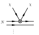
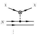
Figure 1: The leading order diagrams for the DM-nucleus scattering. The effective DM–nucleon and DM–meson interactions is denoted by a circle, the dashed lines denote mesons, and the dots represent the remaining $A-2$ nucleon lines.

The LO diagrams for DM-nucleon scattering are shown in Fig. 1. The left diagram gives the leading contribution for the hadronization of the $\bar{q}\gamma_{\mu}q$, $\bar{q}q$, and $GG$ currents. The right diagram is the leading contribution for the hadronization of the $\bar{q}i\gamma_{5}q$ current (the insertion is the mesonic $J^{P}$ current), in which case the left diagram is absent. Finally, for $\bar{q}\gamma_{\mu}\gamma_{5}q$ and $G\tilde{G}$ both the left and the right diagrams are leading and contribute at the same order (for $J_{\chi}^{V}\negthinspace\cdot\negthinspace J_{q}^{A}$ the left diagram dominates). In terms of the $p^{\nu}$ scaling we have for the leading contributions proportional to the $\hat{\cal C}_{a}^{(n,m)}$ Wilson coefficients

$$\begin{split}\nu_{\rm min}&=\nu_{\rm LO}[J_{\chi}^{V}\negthinspace\cdot\negthinspace\tilde{J}_{q}^{V}]=\nu_{\rm LO}[J_{\chi}^{A}\negthinspace\cdot\negthinspace\tilde{J}_{q}^{A}]=\nu_{\rm LO}[J_{\chi}^{S}\tilde{J}^{G}],\\ \nu_{\rm min}+1&=\nu_{\rm LO}[J_{\chi}^{V}\negthinspace\cdot\negthinspace\tilde{J}_{q}^{A}]=\nu_{\rm LO}[J_{\chi}^{A}\negthinspace\cdot\negthinspace\tilde{J}_{q}^{V}]=\nu_{\rm LO}[J_{\chi}^{P}\tilde{J}^{G}]=\nu_{\rm LO}[J_{\chi}^{S}\tilde{J}^{\theta}]=\nu_{\rm LO}[J_{\chi}^{S}J_{q}^{P}],\\ \nu_{\rm min}+2&=\nu_{\rm LO}[J_{\chi}^{S}\tilde{J}_{q}^{S}]\,\,\,\,=\,\,\nu_{\rm LO}[J_{\chi}^{P}\tilde{J}^{\theta}]\,=\nu_{\rm LO}[J_{\chi}^{P}J_{q}^{P}],\\ \nu_{\rm min}+3&=\nu_{\rm LO}[J_{\chi}^{P}\tilde{J}_{q}^{S}].\end{split}$$ (136)

Here $\nu_{\rm min}=3-3A$ simply reflects our normalization of the $A$-nucleon state, where $A$ is the atomic number of the nucleus. In the brackets we displayed the leading products of currents that multiply the $\hat{\cal C}_{a}^{(n,m)}$ in Eqs. (129)-(132). As already mentioned above, for most products of currents the left diagram in Fig. 1 gives the dominant contribution. The resulting $p^{\nu_{\rm LO}}$ suppression then follows directly from the chiral suppression of the corresponding interaction Lagrangian, ${\cal L}_{\chi,{\rm HBChPT}}^{(0,1,2,3)}$. The exceptions are $J_{\chi}^{S}J_{q}^{P}$ and $J_{\chi}^{P}J_{q}^{P}$, for which the right diagram in Fig. 1 dominates. These products have a chiral suppression that is smaller than naively expected from the dimensionality of the corresponding term in ${\cal L}_{\chi,{\rm HBChPT}}^{(0,1,2,3)}$ since the single pion exchange reduces $\nu_{\rm LO}$ by one. From the general counting rule (135) a similar conclusion would be reached also for the product $J_{\chi}^{V}\negthinspace\cdot\negthinspace\tilde{J}_{q}^{A}$. However, in this case the single pion coupling to the DM current vanishes due to vector current conservation, so that the formally leading contribution from the right diagram in Fig. 1 is zero. Special cases are $J_{\chi}^{A}\negthinspace\cdot\negthinspace\tilde{J}_{q}^{A}$, $J_{\chi}^{P}\negthinspace\cdot\negthinspace\tilde{J}_{q}^{\theta}$, and $J_{\chi}^{S}\negthinspace\cdot\negthinspace\tilde{J}_{q}^{\theta}$, for which both diagrams in Fig. 1 contribute at the same order.

Note that at LO in chiral counting DM interacts with a single nucleon, either directly through the short distance operator, or through a single pion exchange. An interesting question is at which order in $p$ the two-body interactions do become important. Examples of the relevant subleading contributions are shown in Fig. 2. The first two diagrams are due to DM coupling to a short distance two-nucleon current. These contributions always scale as $p^{\nu_{\rm LO}+3}$. There are also contributions, shown in the third diagram of Fig. 2, where the DM attaches to the meson exchanged between two nucleons, leading to long-distance two-nucleon currents. For DM interactions originating from ${\cal O}_{2,q}^{(6)}\sim J_{\chi}^{A}\negthinspace\cdot\negthinspace J_{q}^{V}$, ${\cal O}_{5,q}^{(7)}\sim J_{\chi}^{S}\negthinspace\cdot\negthinspace J_{q}^{S}$, and ${\cal O}_{6,q}^{(7)}\sim J_{\chi}^{P}\negthinspace\cdot\negthinspace J_{q}^{S}$, this contribution scales as $p^{\nu_{\rm LO}+1}$, while for DM interactions originating from ${\cal O}_{1,q}^{(6)}\sim J_{\chi}^{V}\negthinspace\cdot\negthinspace J_{q}^{V}$ it scales as $p^{\nu_{\rm LO}+2}$. In these cases the long distance two-nucleon contributions are parametrically larger than the short distance ones. For the remaining operators the long-distance contributions are of the same order or power suppressed compared to the short-distance ones.

In addition, there are higher-order corrections that involve single-nucleon interactions with DM. The last diagram in Fig. 2 shows an example of such an one-loop contribution. In addition there are also power suppressed single-nucleon current insertions. These include the counterterms that cancel the 1-loop divergences. For the DM interactions $J_{\chi}^{A}\negthinspace\cdot\negthinspace J_{q}^{V}$, $J_{\chi}^{S}\negthinspace\cdot\negthinspace J_{q}^{S}$, and $J_{\chi}^{P}\negthinspace\cdot\negthinspace J_{q}^{S}$, the one-loop contributions scale as $p^{\nu_{\rm LO}+1}$, and are, together with the long-distance pion exchange from the third diagram in Fig. 2, the leading chiral corrections.

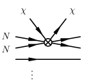
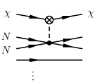
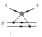
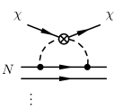
Figure 2: Sample NLO diagrams for the DM-nucleon scattering inside nuclei. The effective DM–nucleon or DM–meson interaction is denoted by a box, the dashed lines denote mesons.

In this work we are satisfied with LO matching and neglect relative ${\mathcal{O}}(p)$-suppressed terms. Our results thus have a relative ${\mathcal{O}}(q/\Lambda_{\rm ChEFT})\sim 30\%$ accuracy. At this order the effective DM interactions involve only single nucleon currents. At NLO, i.e., at relative ${\mathcal{O}}((q/\Lambda_{\rm ChEFT})^{2})\sim 10\%$ accuracy, the DM is still interacting with a single nucleon current for almost all DM–nucleon effective operators. The exceptions are the DM–nucleon interactions $J_{\chi}^{A}\negthinspace\cdot\negthinspace J_{q}^{V}$, $J_{\chi}^{S}\negthinspace\cdot\negthinspace J_{q}^{S}$, and $J_{\chi}^{P}\negthinspace\cdot\negthinspace J_{q}^{S}$. For these the two-nucleon contributions are a long-distance effect so that the corrections are still calculable in ChPT. The results for scalar quark currents in the case of Xe are available in Cirigliano et al. (2012); Hoferichter et al. (2015), and are of the expected size. The genuine short-distance two-nucleon currents, for which one would require lattice QCD calculations, appear only at NNNLO in chiral counting, i.e., below few-percent accuracy.

IV.2 Form factors for dark matter–nucleon interactions

We can use the formalism in the previous section to calculate the form factors for the DM–nucleon interactions. We perform the leading order matching, shown in Fig. 1. The hadronized $\bar{q}\gamma_{\mu}q$, $\bar{q}q$, $G\tilde{G}$, and $GG$ currents receive contributions from the left diagram, the $\bar{q}i\gamma_{5}q$ current from the right diagram, while $\bar{q}\gamma_{\mu}\gamma_{5}q$ receives contributions from both diagrams. The expanded hadronic currents are collected in Appendix B.4. We include the contributions from single $\pi^{0}$ and $\eta$ exchanges in the $q^{2}$-dependent coefficients of the nonrelativistic operators defined below. The momenta exchanges are small enough that the DM-nucleon interactions cannot lead to the dissociation of nuclei and the production of on-shell pions.

The resulting effective Lagrangian is

$${\cal L}_{\rm eff}=\sum_{i,d}\Big{(}c_{i,p}^{(d)}(q^{2})\,Q_{i,p}^{(d)}+c_{i,n}^{(d)}(q^{2})\,Q_{i,n}^{(d)}\Big{)},$$ (137)

with $d$ counting the number of derivatives in the operators. It is understood that ${\cal L}_{\rm eff}$ is to be used only at tree level. The operator basis is, for $d=0$,

$$Q_{1,p}^{(0)} =\big{(}\bar{\chi}_{v}\chi_{v}\big{)}\big{(}\bar{p}_{v}p_{v}\big{)}, Q_{2,p}^{(0)} =\big{(}\bar{\chi}_{v}S_{\chi}^{\mu}\chi_{v}\big{)}\big{(}\bar{p}_{v}S_{N,\mu}p_{v}\big{)},$$ (138)

with a similar set of operators for neutrons, with $p\to n$. The $Q_{1,p}^{(0)}$ operator will induce spin-independent DM scattering on the nucleus, while $Q_{2,p}^{(0)}$ will induce the spin-dependent scattering. In our analysis we also include all the $d=1$ operators,

$$Q_{1,p}^{(1)} =\big{(}\bar{\chi}_{v}\chi_{v}\big{)}\big{(}\bar{p}_{v}iq\negthinspace\cdot\negthinspace S_{N}p_{v}\big{)}, Q_{2,p}^{(1)} =\big{(}\bar{\chi}_{v}iq\negthinspace\cdot\negthinspace S_{\chi}\chi_{v}\big{)}\big{(}\bar{p}_{v}p_{v}\big{)},$$ (139)

$$Q_{3,p}^{(1)} =m_{N}\big{(}\bar{\chi}_{v}\chi_{v}\big{)}\big{(}\bar{p}_{v}\,v_{\perp}\negthinspace\cdot\negthinspace S_{N}\,p_{v}\big{)}, Q_{4,p}^{(1)} =m_{N}\big{(}\bar{\chi}_{v}\,v_{\perp}\negthinspace\cdot\negthinspace S_{\chi}\,\chi_{v}\big{)}\big{(}\bar{p}_{v}p_{v}\big{)},$$ (140)

$$Q_{5,p}^{(1)} =i\epsilon^{\alpha\beta\mu\nu}v_{\alpha}q_{\beta}\big{(}\bar{\chi}_{v}S_{\chi,\mu}\chi_{v}\big{)}\big{(}\bar{p}_{v}S_{N,\nu}p_{v}\big{)}, Q_{6,p}^{(1)} =m_{N}\epsilon^{\alpha\beta\mu\nu}v_{\alpha}v_{\perp,\beta}\big{(}\bar{\chi}_{v}S_{\chi,\mu}\chi_{v}\big{)}\big{(}\bar{p}_{v}S_{N,\nu}p_{v}\big{)}.$$ (141)

The related operators for neutrons are obtained with a $p\to n$ replacement. From the $d=2$ set of operators we need only

$$Q_{1,p}^{(2)} =\big{(}\bar{\chi}_{v}iq\negthinspace\cdot\negthinspace S_{\chi}\chi_{v}\big{)}\big{(}\bar{p}_{v}\,iq\negthinspace\cdot\negthinspace S_{N}\,p_{v}\big{)}, Q_{2,p}^{(2)} =im_{N}\,\epsilon^{\alpha\beta\mu\nu}v_{\alpha}q_{\beta}v_{\perp,\mu}\big{(}\bar{\chi}_{v}S_{\chi,\nu}\chi_{v}\big{)}\big{(}\bar{p}_{v}p_{v}\big{)}.$$ (142)

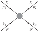
Figure 3: The kinematics of DM scattering on nucleons, $\chi(p_{1})N(k_{1})\to\chi(p_{2})N(k_{2})$.

Above, we have defined several kinematic quantities for DM-nucleon scattering, $\chi(p_{1})N(k_{1})\to\chi(p_{2})N(k_{2})$, see Fig. 3. The momentum exchange is

$$q^{\mu}\equiv k_{2}^{\mu}-k_{1}^{\mu}=p_{1}^{\mu}-p_{2}^{\mu},\qquad q^{\mu}=\big{(}q^{0},\vec{q}\big{)}.$$ (143)

The definition of momentum exchange three vector is thus

$$\vec{q}=\vec{k}_{2}-\vec{k}_{1}=\vec{p}_{1}-\vec{p}_{2}.$$ (144)

It is also useful to define the four-component perpendicular relative velocity (see also Anand et al. (2014))

$$v_{\perp}^{\mu}=\frac{1}{2}\Big{(}\frac{p_{1}^{\mu}}{m_{\chi}}+\frac{p_{2}^{\mu}}{m_{\chi}}-\frac{k_{1}^{\mu}}{m_{N}}-\frac{k_{2}^{\mu}}{m_{N}}\Big{)}=\Delta v^{\mu}-\frac{q^{\mu}}{2\mu_{N}}\,,$$ (145)

where $\Delta v^{\mu}$ is the initial relative velocity between DM and nucleon,

$$\Delta v^{\mu}=\frac{p_{1}^{\mu}}{m_{\chi}}-\frac{k_{1}^{\mu}}{m_{N}},$$ (146)

and $\mu_{N}=m_{\chi}m_{N}/(m_{\chi}+m_{N})$ the reduced mass of the DM–nucleon system (we work in the isospin limit, $m_{N}=m_{p}=m_{n}$). Note the difference in our notation between $v^{\mu}$, the HBChPT velocity label, and $\Delta v^{\mu}$, the initial relative velocity. In the lab frame we have $v^{\mu}=(1,\vec{0}\,)$, while $\Delta v^{\mu}\sim{\mathcal{O}}(\Lambda_{\rm QCD}/m_{N})$ arises primarily due to the movement of nucleons inside the nucleus. The perpendicular relative velocity obeys $v_{\perp}\cdot q=0$. Furthermore, in the lab frame one has $v_{\perp}^{\mu}=(0,\vec{v}_{\perp})$ so that also $\vec{v}_{\perp}\cdot\vec{q}=0$.

The $d=0$ Wilson coefficients for interactions of DM with protons are given by

$$\begin{split}c_{1,p}^{(0)}&=2\,\hat{\cal C}_{1,u}^{(6,0)}+\hat{\cal C}_{1,d}^{(6,0)}-\frac{2m_{G}}{27}\,\hat{\cal C}_{1}^{(7,0)}+\sigma_{u}^{p}\,\hat{\cal C}_{5,u}^{(7,0)}+\sigma_{d}^{p}\,\hat{\cal C}_{5,d}^{(7,0)}+\sigma_{s}\hat{\cal C}_{5,s}^{(7,0)}-\frac{\alpha Q_{p}}{2\pi m_{\chi}}\hat{\cal C}_{1}^{(5,0)}\,,\end{split}$$ (147)

$$\begin{split}c_{2,p}^{(0)}&=4\big{(}\,\Delta u_{p}\,\hat{\cal C}_{4,u}^{(6,0)}+\,\Delta d_{p}\,\hat{\cal C}_{4,d}^{(6,0)}+\Delta s\,\hat{\cal C}_{4,s}^{(6,0)}\big{)}+\frac{2\alpha}{\pi}\frac{\mu_{p}}{m_{N}}\hat{\cal C}_{1}^{(5,0)}\,,\end{split}$$ (148)

while the contributions for the neutrons are obtained through the replacement $p\to n$, $u\leftrightarrow d$. For convenience of notation we assumed that HDMET matching was done at tree level (see the end of this Section for the general case). The above results can then be used directly also for the relativistic form of the DM EFT (3)-(9) by simply replacing $\hat{C}_{i}^{(d,0)}\to\hat{C}_{i}^{(d)}$. The terms proportional to $\hat{\cal C}_{1}^{(5,0)}$ come from a single photon exchange. For the photon propagator we used that $v\cdot q={\mathcal{O}}(q^{2})$, so that $(q^{2}-(v\cdot q)^{2})/q^{2}=1+{\mathcal{O}}(q^{2})$. The low-energy constant $m_{G}$ is the gluon contribution to the nucleon mass. The remaining HBChPT constants have been converted to nucleon sigma terms, $\sigma_{u,d}^{p}$, axial vector matrix elements, $\Delta q_{p}$, and nuclear magnetic moments, $\mu_{N}$, using the leading-order expressions in Appendix C. Their values are given in Appendix C and are collected in Tab. 2. $Q_{p(n)}=1(0)$ is the proton (neutron) electric charge.

LE constant	value	LE constant	value	LE constant	value
$\Delta u_{p}=\Delta d_{n}$	$0.897(27)$	$\Delta d_{p}=\Delta u_{n}$	$-0.376(27)$	$\Delta s$	$-0.026(4)$
$\mu_{p}$	$2.79$	$\mu_{n}$	$-1.91$	$\mu_{s}$	$-0.073(19)$
$B_{0}m_{u}$	$(6200\pm 400)\,\text{MeV}^{2}$	$B_{0}m_{d}$	$(13300\pm 400)\,\text{MeV}^{2}$	$B_{0}m_{s}$	$(0.27\pm 0.01)\,\text{GeV}^{2}$
$\sigma_{u}^{p}$	$(17\pm 5)\,\text{MeV}$	$\sigma_{d}^{p}$	$(32\pm 10)\,\text{MeV}$	$\sigma_{s}$	$(41.3\pm 7.7)\,\text{MeV}$
$\sigma_{u}^{n}$	$(15\pm 5)\,\text{MeV}$	$\sigma_{d}^{n}$	$(36\pm 10)\,\text{MeV}$
$g_{A}$	$1.2723(23)$	$m_{G}$	$848(14)\,$MeV

Table 2: Numerical input values for the non-perturbative constants. For more details and references, see Appendix C.

The $d=1$ Wilson coefficients are

$$\begin{split}c_{1,p}^{(1)}&=\frac{B_{0}\,g_{A}}{m_{\pi}^{2}-q^{2}}\big{(}m_{u}\hat{\cal C}_{7,u}^{(7,0)}-m_{d}\hat{\cal C}_{7,d}^{(7,0)}\big{)}\\ &\quad+\frac{B_{0}}{3}\frac{(\Delta u_{p}+\Delta d_{p}-2\Delta s)}{m_{\eta}^{2}-q^{2}}\big{(}m_{u}\hat{\cal C}_{7,u}^{(7,0)}+m_{d}\hat{\cal C}_{7,d}^{(7,0)}-2m_{s}\hat{\cal C}_{7,s}^{(7,0)}\big{)}\\ &\quad-\tilde{m}\bigg{[}\frac{\Delta u_{p}}{m_{u}}+\frac{\Delta d_{p}}{m_{d}}+\frac{\Delta s}{m_{s}}+\frac{g_{A}}{2}\bigg{(}\frac{1}{m_{u}}-\frac{1}{m_{d}}\bigg{)}\frac{q^{2}}{m_{\pi}^{2}-q^{2}}\\ &\qquad\quad+\frac{1}{6}\big{(}\Delta u_{p}+\Delta d_{p}-2\Delta s\big{)}\bigg{(}\frac{1}{m_{u}}+\frac{1}{m_{d}}-\frac{2}{m_{s}}\bigg{)}\frac{q^{2}}{m_{\eta}^{2}-q^{2}}\bigg{]}\hat{\cal C}_{3}^{(7,0)}\,,\end{split}$$ (149)

$$\begin{split}c_{2,p}^{(1)}&=-\sigma_{u}^{p}\hat{\cal C}_{6,u}^{(8,1)}-\sigma_{d}^{p}\hat{\cal C}_{6,d}^{(8,1)}-\sigma_{s}\hat{\cal C}_{6,s}^{(8,1)}+\frac{2m_{G}}{27}\hat{\cal C}_{2}^{(8,1)}-\frac{2\alpha Q_{p}}{\pi q^{2}}\hat{\cal C}_{2}^{(5,0)}\,,\end{split}$$ (150)

$$c_{3,p}^{(1)} =\frac{2}{m_{N}}\Big{[}\Delta u_{p}\,\hat{\cal C}_{3,u}^{(6,0)}+\Delta d_{p}\,\hat{\cal C}_{3,d}^{(6,0)}+\Delta s\,\hat{\cal C}_{3,s}^{(6,0)}\Big{]}\,,$$ (151)

$$c_{4,p}^{(1)} =-\frac{2}{m_{N}}\Big{[}2\,\hat{\cal C}_{2,u}^{(6,0)}+\,\hat{\cal C}_{2,d}^{(6,0)}\Big{]},$$ (152)

$$\begin{split}c_{5,p}^{(1)}&=\frac{4\hat{\mu}_{u}^{p}}{m_{N}}\hat{\cal C}_{2,u}^{(6,0)}+\frac{2\hat{\mu}_{d}^{p}}{m_{N}}\hat{\cal C}_{2,d}^{(6,0)}-\frac{6}{m_{N}}\mu_{s}\,\hat{\cal C}_{2,s}^{(6,0)}\\ &\quad+\frac{2}{m_{\chi}}\Big{(}\Delta u_{p}\,\hat{\cal C}_{3,u}^{(6,0)}+\Delta d_{p}\,\hat{\cal C}_{3,d}^{(6,0)}+\Delta s\,\hat{\cal C}_{3,s}^{(6,0)}\Big{)}\,,\end{split}$$ (153)

$$c_{6,p}^{(1)} =0\,,$$ (154)

while the Wilson coefficients for the interactions of DM with neutrons, $c_{i}^{n}$, are obtained by the replacements $p\to n,u\leftrightarrow d$. We have defined

$$\tilde{m}=\bigg{(}\frac{1}{m_{u}}+\frac{1}{m_{d}}+\frac{1}{m_{s}}\bigg{)}^{-1}\,.$$ (155)

The above results apply to the relativistic form of the DM EFT (3)-(9) by replacing $\hat{C}_{i}^{(d,0)}\to\hat{C}_{i}^{(d)}$ and $\hat{C}_{i}^{(8,1)}\to\hat{C}_{i}^{(7)}$, as long as the matching to HDMET was performed at tree level (see the end of this Section for the general case). In Eq. (149) and in Eq. (156) below we use $\Delta u_{p}-\Delta d_{p}=\Delta d_{n}-\Delta u_{n}=g_{A}$ as this combination is determined more precisely, see Eq. (304). The $B_{0}$ coefficient is related to the quark condensate so that $B_{0}m_{q}\sim m_{\pi}^{2}$, see Eq. (315). We have also defined the contributions to the proton and neutron magnetic moments from the $u$- and $d$-quark currents, $\hat{\mu}_{u}^{p}=\hat{\mu}_{d}^{n}=1.84,\hat{\mu}_{d}^{p}=\hat{\mu}_{u}^{n}=-1.03$ (see Eq. (314)), while $\mu_{s}$ is the $s$ quark contribution to the proton and neutron magnetic moments, see Eq. (311).

The $d=2$ Wilson coefficients are

$$\begin{split}c_{1,p}^{(2)}&=\frac{2\alpha}{\pi q^{2}}\frac{\mu_{p}}{m_{N}}\,\hat{\cal C}_{1}^{(5,0)}-\frac{2}{3}\frac{(\Delta u_{p}+\Delta d_{p}-2\Delta s)}{m_{\eta}^{2}-q^{2}}\Big{(}\hat{\cal C}_{4,u}^{(6,0)}+\hat{\cal C}_{4,d}^{(6,0)}-2\hat{\cal C}_{4,s}^{(6,0)}\Big{)}\\ &\quad-\frac{2g_{A}}{m_{\pi}^{2}-q^{2}}\Big{(}\hat{\cal C}_{4,u}^{(6,0)}-\hat{\cal C}_{4,d}^{(6,0)}\Big{)}+\frac{B_{0}}{m_{\chi}}\frac{g_{A}}{m_{\pi}^{2}-q^{2}}\big{(}m_{u}\,\hat{\cal C}_{8,u}^{(7,0)}-m_{d}\,\hat{\cal C}_{8,d}^{(7,0)}\big{)}\\ &\quad+\frac{B_{0}}{3m_{\chi}}\frac{(\Delta u_{p}+\Delta d_{p}-2\Delta s)}{m_{\eta}^{2}-q^{2}}\big{(}m_{u}\,\hat{\cal C}_{8,u}^{(7,0)}+m_{d}\,\hat{\cal C}_{8,d}^{(7,0)}-2m_{s}\hat{\cal C}_{8,s}^{(7,0)}\big{)}\\ &\quad+\tilde{m}\bigg{[}\frac{\Delta u_{p}}{m_{u}}+\frac{\Delta d_{p}}{m_{d}}+\frac{\Delta s}{m_{s}}+\frac{g_{A}}{2}\bigg{(}\frac{1}{m_{u}}-\frac{1}{m_{d}}\bigg{)}\frac{q^{2}}{m_{\pi}^{2}-q^{2}}\\ &\qquad\quad+\frac{1}{6}\big{(}\Delta u_{p}+\Delta d_{p}-2\Delta s\big{)}\bigg{(}\frac{1}{m_{u}}+\frac{1}{m_{d}}-\frac{2}{m_{s}}\bigg{)}\frac{q^{2}}{m_{\eta}^{2}-q^{2}}\bigg{]}\hat{\cal C}_{4}^{(8,1)},\end{split}$$ (156)

$$c_{2,p}^{(2)} =-\frac{2\alpha Q_{p}}{\pi m_{N}q^{2}}\,\hat{\cal C}_{1}^{(5,0)},$$ (157)

while the expressions for the neutron follow from the replacements $p\to n,u\leftrightarrow d$. As before the above results also apply to the relativistic form of the DM EFT (3)-(9) by replacing $\hat{C}_{i}^{(d,0)}\to\hat{C}_{i}^{(d)}$, $\hat{\cal C}_{4}^{(8,1)}\to\hat{\cal C}_{4}^{(7)}/m_{\chi}$ (for tree level matching to HDMET). Note that, due to the photon $1/q^{2}$ pole, the $\hat{\cal C}_{1}^{(5,0)}$ contributions are of the same order as in (147), (149), even though they multiply operators that are ${\mathcal{O}}(q^{2})$ suppressed. Similarly, due to the meson poles, the contributions proportional to the Wilson coefficients $\hat{\cal C}_{4,q}^{(6,0)}$ in $c_{1,p}^{(2)}$, coming from the right diagram in Fig. 1 are of the same chiral order as the $\hat{\cal C}_{4,q}^{(6,0)}$ terms in $c_{2,p}^{(0)}$, coming from the left diagram in Fig. 1.

The coefficients $c_{1,N}^{(1)}$, $c_{2,p}^{(1)}$, $c_{1,N}^{(2)}$ have a $q^{2}$-dependence from pion, $\eta$, and photon exchanges, i.e., they are non-local at the scale $q\sim m_{\pi}$. This signals that the above effective description of DM–nucleon interactions is not an effective field theory in the usual sense, and ${\cal L}_{\rm eff}$ from (137) may only be used at tree level. The effective description does make sense, though, since the pion and the $\eta$ cannot be kinematically produced and never appear as asymptotic states. In the scattering process $q^{2}$ is spacelike, so that one never reaches the pion or $\eta$ pole in the above expressions. The single photon exchange similarly leads to a classical potential for the DM-proton interactions.

The above results apply with trivial changes also if the matching to HDMET is performed beyond tree level. In that case one needs to replace $\hat{\cal C}_{1}^{(5,0)}\to m_{\chi}\hat{\cal C}_{2}^{(6,1)}$ in (147), $\hat{\cal C}_{1}^{(5,0)}\to m_{\chi}\hat{\cal C}_{1}^{(6,1)}$ in (157), $\hat{\cal C}_{3,q}^{(6,0)}\to m_{\chi}\hat{\cal C}_{3,q}^{(7,1)}$ in (151), $\hat{\cal C}_{3,q}^{(6,0)}\to m_{\chi}\hat{\cal C}_{6,q}^{(7,1)}$ in (153), $\hat{\cal C}_{8,q}^{(7,0)}\to m_{\chi}\hat{\cal C}_{8,q}^{(8,1)}$ in (156).

Using the results of Ref. Anand et al. (2014) for the nuclear response in DM direct detection, the cross section for DM scattering on the nucleus is given by

$$\frac{d\sigma}{dE_{R}}=\frac{m_{A}}{2\pi|\vec{v}_{\chi}|^{2}}\frac{1}{(2J_{\chi}+1)}\frac{1}{(2J_{A}+1)}\sum_{\rm spins}|{\cal M}|_{\rm NR}^{2},$$ (158)

where $E_{R}$ is the recoil energy of the nucleus, $m_{A}$ its mass, and $\vec{v}_{\chi}$ the initial DM velocity in the lab frame. The non-vanishing contributions to the matrix element squared are Anand et al. (2014)

$$\begin{split}\frac{1}{2J_{\chi}+1}\,\frac{1}{2J_{A}+1}\sum_{\rm spins}|{\cal M}|_{\rm NR}^{2}=&\frac{4\pi}{2J_{A}+1}\sum_{\tau=0,1}\sum_{\tau^{\prime}=0,1}\Big{\{}R_{M}^{\tau\tau^{\prime}}W_{M}^{\tau\tau^{\prime}}(q)+R_{\Sigma^{\prime\prime}}^{\tau\tau^{\prime}}W_{\Sigma^{\prime\prime}}^{\tau\tau^{\prime}}(q)\\ +&R_{\Sigma^{\prime}}^{\tau\tau^{\prime}}W_{\Sigma^{\prime}}^{\tau\tau^{\prime}}(q)+\frac{\vec{q}^{\,\,2}}{m_{N}^{2}}\Big{[}R_{\Delta}^{\tau\tau^{\prime}}W_{\Delta}^{\tau\tau^{\prime}}(q)+R_{\Delta\Sigma^{\prime}}^{\tau\tau^{\prime}}W_{\Delta\Sigma^{\prime}}^{\tau\tau^{\prime}}(q)\Big{]}\Big{\}},\end{split}$$ (159)

where $J_{\chi}=1/2$ is the spin of DM, and $J_{A}$ is the spin of the target nucleus. The nonrelativistic matrix element ${\cal M}_{\rm NR}$ has the same normalization as the one in Anand et al. (2014). The coefficients $R_{i}^{\tau\tau^{\prime}}$ depend on $\vec{v}_{T}^{\perp 2}$, $\vec{q}^{\,\,2}/m_{N}^{2}$, as well as on the coefficients $c_{i,N}^{(d)}$ in (147)-(157), and are given by Anand et al. (2014)

$$\begin{split}R_{M}^{\tau\tau^{\prime}}&=c_{1,\tau}^{(0)}c_{1,\tau^{\prime}}^{(0)}+\frac{m_{N}^{2}}{4}\Big{[}\frac{\vec{q}^{\,\,2}}{m_{N}^{2}}c_{2,\tau}^{(1)}c_{2,\tau^{\prime}}^{(1)}+\vec{v}_{T}^{\perp 2}\Big{(}c_{4,\tau}^{(1)}c_{4,\tau^{\prime}}^{(1)}+\vec{q}^{\,\,2}c_{2,\tau}^{(2)}c_{2,\tau^{\prime}}^{(2)}\Big{)}\Big{]},\end{split}$$ (160)

$$\begin{split}R_{\Sigma^{\prime\prime}}^{\tau\tau^{\prime}}&=\frac{1}{16}\Big{[}c_{2,\tau}^{(0)}c_{2,\tau^{\prime}}^{(0)}+\vec{q}^{\,\,2}\Big{(}c_{2,\tau}^{(0)}c_{1,\tau^{\prime}}^{(2)}+c_{1,\tau}^{(2)}c_{2,\tau^{\prime}}^{(0)}+4c_{1,\tau}^{(1)}c_{1,\tau^{\prime}}^{(1)}\Big{)}+\vec{q}^{\,\,4}c_{1,\tau}^{(2)}c_{1,\tau^{\prime}}^{(2)}\Big{]},\end{split}$$ (161)

$$R_{\Sigma^{\prime}}^{\tau\tau^{\prime}} =\frac{m_{N}^{2}}{8}\vec{v}_{T}^{\perp 2}\,c_{3,\tau}^{(1)}c_{3,\tau^{\prime}}^{(1)}+\frac{1}{16}\Big{(}c_{2,\tau}^{(0)}c_{2,\tau^{\prime}}^{(0)}+\vec{q}^{\,\,2}c_{5,\tau}^{(1)}c_{5,\tau^{\prime}}^{(1)}\Big{)},$$ (162)

$$R_{\Delta}^{\tau\tau^{\prime}} =\frac{m_{N}^{2}}{4}\Big{(}c_{4,\tau}^{(1)}c_{4,\tau^{\prime}}^{(1)}+\vec{q}^{\,\,2}c_{2,\tau}^{(2)}c_{2,\tau^{\prime}}^{(2)}\Big{)},$$ (163)

$$R_{\Delta\Sigma^{\prime}}^{\tau\tau^{\prime}} =\frac{m_{N}^{2}}{4}\Big{(}c_{4,\tau}^{(1)}c_{5,\tau^{\prime}}^{(1)}-c_{2,\tau}^{(2)}c_{2,\tau^{\prime}}^{(0)}\Big{)}.$$ (164)

Note that (160)-(164) are already specific to the case of fermionic DM, $J_{\chi}=1/2$ (see Anand et al. (2014) for the general expression). Above,

$$\vec{v}_{T}^{\perp}=\vec{v}_{\chi}-\vec{q}/(2\mu_{\chi A}),$$ (165)

is the component of initial DM velocity in the lab frame, $\vec{v}_{\chi}$, that is perpendicular to $\vec{q}$, in complete analogy with the single nucleon case (145). The typical value is $|\vec{v}_{T}^{\perp}|\sim 10^{-3}$. Here $\mu_{\chi A}=1/(1/m_{\chi}+1/m_{A})$ is the reduced mass of the DM and the nucleus. The sum in (159) is over isospin values $\tau=0,1$. The Wilson coefficients $c_{i,\tau}^{(d)}$ are related to the proton and neutron Wilson coefficients through

$$c_{i,0}^{(d)}=\frac{1}{2}\big{(}c_{i,p}^{(d)}+c_{i,n}^{(d)}\big{)},\qquad c_{i,1}^{(d)}=\frac{1}{2}\big{(}c_{i,p}^{(d)}-c_{i,n}^{(d)}\big{)}\,.$$ (166)

V Scalar dark matter

The above results are easily extended to the case of scalar DM. For relativistic scalar DM, denoted by $\varphi$, the effective interactions with the SM start at dimension six,

$${\cal L}_{\varphi}=\hat{\cal C}_{a}^{(6)}{\cal Q}_{a}^{(6)}+\cdots,\qquad{\rm where}\quad\hat{\cal C}_{a}^{(6)}=\frac{{\cal C}_{a}^{(6)}}{\Lambda^{2}}\,,$$ (167)

where ellipses denote higher dimension operators. The dimension-six operators are

$${\cal Q}_{1,q}^{(6)} =\big{(}\varphi^{*}i\overset{\leftrightarrow}{\partial_{\mu}}\varphi\big{)}(\bar{q}\gamma^{\mu}q), {\cal Q}_{2,q}^{(6)} =\big{(}\varphi^{*}i\overset{\leftrightarrow}{\partial_{\mu}}\varphi\big{)}(\bar{q}\gamma^{\mu}\gamma_{5}q),$$ (168)

$${\cal Q}_{3,q}^{(6)} =m_{q}(\varphi^{*}\varphi)(\bar{q}q)\,, {\cal Q}_{4,q}^{(6)} =m_{q}(\varphi^{*}\varphi)(\bar{q}i\gamma_{5}q)\,,$$ (169)

$${\cal Q}_{5}^{(6)} =\frac{\alpha_{s}}{12\pi}(\varphi^{*}\varphi)G^{a\mu\nu}G_{\mu\nu}^{a}\,, {\cal Q}_{6}^{(6)} =\frac{\alpha_{s}}{8\pi}(\varphi^{*}\varphi)G^{a\mu\nu}\widetilde{G}_{\mu\nu}^{a}\,.$$ (170)

$${\cal Q}_{7}^{(6)} =i\frac{e}{8\pi^{2}}\big{(}\partial_{\mu}\varphi^{*}\partial_{\nu}\varphi\big{)}F^{\mu\nu}\,,$$ (171)

Here $\overset{\leftrightarrow}{\partial_{\mu}}$ is defined through $\phi_{1}\overset{\leftrightarrow}{\partial_{\mu}}\phi_{2}=\phi_{1}\partial_{\mu}\phi_{2}-(\partial_{\mu}\phi_{1})\phi_{2}$, and $q=u,d,s$ again denote the light quarks. The strong coupling constant $\alpha_{s}$ is taken at $\mu\sim 1$ GeV. The operator ${\cal Q}_{6}^{(6)}$ is CP-odd, while the other operators are CP-even. Note that because there are also leptonic equivalents to the operators ${\cal Q}_{1,q}^{(6)}$ which we do not include in the analysis, the inclusion of ${\cal Q}_{7}^{(6)}$ is not redundant (the equations of motion relate $\partial^{\mu}F_{\mu\nu}=\sum_{f}eQ_{f}\bar{f}\gamma_{\nu}f$ where $f$ are both quarks and leptons).

In (168)-(171) we kept the leading operators that one would get from a UV theory of complex scalar DM for each of the chiral and flavor structures. At dimension six there are also the Rayleigh operators $(\varphi^{*}\varphi)F^{\mu\nu}F_{\mu\nu}$ and $(\varphi^{*}\varphi)F^{\mu\nu}\widetilde{F}_{\mu\nu}$ which, however, lead to scattering rates suppressed by a factor of $\alpha$ compared to ${\cal Q}_{7}^{(6)}$ Ovanesyan and Vecchi (2015). For real scalar DM the operators ${\cal Q}_{1,q}^{(6)}$, ${\cal Q}_{2,q}^{(6)}$, and ${\cal Q}_{7}^{(6)}$ vanish, and one would need to consider subleading operators. In this paper we limit ourselves to the case of complex scalar DM.

The next step is to consider scalar DM interactions with the visible sector in HDMET. To derive it we factor out the large momenta,

$$\varphi(x)=\frac{1}{\sqrt{2m_{\varphi}}}e^{-im_{\varphi}v\cdot x}\varphi_{v}\,.$$ (172)

The HDMET for scalar DM is thus

$${\cal L}_{\rm HDMET}=\varphi_{v}^{*}iv\negthinspace\cdot\negthinspace\partial\varphi_{v}^{\phantom{*}}+\frac{1}{2m_{\varphi}}\varphi_{v}^{*}(i\partial_{\perp})^{2}\varphi_{v}^{\phantom{*}}+\cdots+{\cal L}_{\varphi_{v}}\,.$$ (173)

The first term is the LO HDMET for scalar fields. The $1/m_{\varphi}$ term is fixed by reparametrization invariance Luke and Manohar (1992), while the ellipses denote the higher-order terms. The interaction Lagrangian ${\cal L}_{\varphi_{v}}$ is also expanded in $1/m_{\varphi}$,

$${\cal L}_{\varphi_{v}}=\sum_{d,m}\hat{\cal C}_{a}^{(d,m)}{\cal Q}_{a}^{(d,m)},\qquad{\rm where}\qquad\hat{\cal C}_{a}^{(d,m)}=\frac{{\cal C}_{a}^{(d,m)}|_{n_{f}=5}}{\Lambda^{d-m-4}m_{\varphi}^{m}}\,.$$ (174)

As for fermionic DM, the operators ${\cal Q}_{a}^{(d,m)}$ arise as the terms of order $1/m_{\chi}^{m}$ in the HDMET expansion of the UV operators ${\cal Q}_{a}^{(d)}$ in (168)-(171). Because of the derivatives acting on scalar fields the index $m$ can also be negative, since

$$i\big{(}\varphi^{*}\overset{\leftrightarrow}{\partial_{\mu}}\varphi\big{)} \to 2m_{\varphi}v_{\mu}\big{(}\varphi_{v}^{*}\varphi_{v}\big{)}+i\big{(}\varphi_{v}^{*}\overset{\leftrightarrow}{\partial_{\mu}}\varphi_{v}\big{)}+\cdots,$$ (175)

$$\big{(}\partial_{[\mu}\varphi^{*}\partial_{\nu]}\varphi\big{)} \to im_{\varphi}v_{[\mu}\partial_{\nu]}\big{(}\varphi_{v}^{*}\varphi_{v}\big{)}+\big{(}\partial_{[\mu}\varphi_{v}^{*}\partial_{\nu]}\varphi_{v}\big{)}+\cdots.$$ (176)

We thus have three HDMET operators that start at dimension five

$${\cal Q}_{1,q}^{(5,-1)} =2(\varphi_{v}^{*}\varphi_{v})(\bar{q}\not{v}q), {\cal Q}_{2,q}^{(5,-1)} =2(\varphi_{v}^{*}\varphi_{v})(\bar{q}\not{v}\gamma_{5}q),$$ (177)

$${\cal Q}_{3}^{(5,-1)} =-\frac{e}{8\pi^{2}}v_{\mu}\partial_{\nu}\big{(}\varphi_{v}^{*}\varphi_{v}\big{)}F^{\mu\nu}.$$ (178)

The relevant dimension-six operators are

$${\cal Q}_{1,q}^{(6,0)} =\big{(}\varphi_{v}^{*}i\overset{\leftrightarrow}{\partial_{\mu}}\varphi_{v}\big{)}(\bar{q}\gamma^{\mu}q), {\cal Q}_{2,q}^{(6,0)} =\big{(}\varphi_{v}^{*}i\overset{\leftrightarrow}{\partial_{\mu}}\varphi_{v}\big{)}(\bar{q}\gamma^{\mu}\gamma_{5}q),$$ (179)

$${\cal Q}_{3,q}^{(6,0)} =m_{q}(\varphi_{v}^{*}\varphi_{v})(\bar{q}q)\,, {\cal Q}_{4,q}^{(6,0)} =m_{q}(\varphi_{v}^{*}\varphi_{v})(\bar{q}i\gamma_{5}q)\,,$$ (180)

$${\cal Q}_{5}^{(6,0)} =\frac{\alpha_{s}}{12\pi}(\varphi_{v}^{*}\varphi_{v})G^{a\mu\nu}G_{\mu\nu}^{a}\,, {\cal Q}_{6}^{(6,0)} =\frac{\alpha_{s}}{8\pi}(\varphi_{v}^{*}\varphi_{v})G^{a\mu\nu}\widetilde{G}_{\mu\nu}^{a}\,,$$ (181)

$${\cal Q}_{7}^{(6,0)} =i\frac{e}{8\pi^{2}}\big{(}\partial_{\mu}\varphi_{v}^{*}\partial_{\nu}\varphi_{v}\big{)}F^{\mu\nu}.$$ (182)

These are simple extensions of the relativistic operators in (168)-(171), but the derivatives are now all ${\mathcal{O}}(q)$ since they act on HDMET fields. Reparametrization invariance fixes

$${\cal C}_{1,q}^{(5,-1)}={\cal C}_{1,q}^{(6,0)}\,,\qquad{\cal C}_{2,q}^{(5,-1)}={\cal C}_{2,q}^{(6,0)}\,,\qquad{\cal C}_{3}^{(5,-1)}={\cal C}_{7}^{(6,0)}$$ (183)

to all loop orders in the matching at the scale $m_{\chi}$. In the Lagrangian (174) the operators thus always appear in the linear combinations

$$\begin{split}m_{\varphi}{\cal Q}_{1,q}^{(5,-1)}+{\cal Q}_{1,q}^{(6,0)},\qquad m_{\varphi}{\cal Q}_{2,q}^{(5,-1)}+{\cal Q}_{2,q}^{(6,0)},\qquad m_{\varphi}{\cal Q}_{3}^{(5,-1)}+{\cal Q}_{7}^{(6,0)}.\end{split}$$ (184)

It is now easy to obtain the ChPT and HBChPT Lagrangians. The external spurions in the QCD Lagrangian (38) are, for relativistic DM,

$$\nu_{\mu}(x) =-e\bar{Q}_{q}A_{\mu}^{e}+\nu_{\chi,\mu}=-e\bar{Q}_{q}A_{\mu}^{e}+\bar{\cal C}_{1}^{(6)}\big{(}\varphi^{*}i\overset{\leftrightarrow}{\partial_{\mu}}\varphi\big{)},$$ (185)

$$a_{\mu}(x) =\bar{\cal C}_{2}^{(6)}\big{(}\varphi^{*}i\overset{\leftrightarrow}{\partial_{\mu}}\varphi\big{)},$$ (186)

$$s(x) ={\cal M}_{q}+s_{\chi}={\cal M}_{q}-{\cal M}_{q}\,\bar{\cal C}_{3}^{(6)}\big{(}\varphi^{*}\varphi\big{)},$$ (187)

$$p(x) ={\cal M}_{q}\,\bar{\cal C}_{4}^{(6)}\big{(}\varphi^{*}\varphi\big{)},$$ (188)

$$s_{G}(x) =\hat{\cal C}_{5}^{(6)}\big{(}\varphi^{*}\varphi\big{)},$$ (189)

$$\theta(x) =\hat{\cal C}_{6}^{(6)}\big{(}\varphi^{*}\varphi\big{)}.$$ (190)

For HDMET the external spurions are thus

$$\nu_{\mu}(x) =-e\bar{Q}_{q}A_{\mu}^{e}+\nu_{\chi,\mu}=-e\bar{Q}_{q}A_{\mu}^{e}+2v^{\mu}\bar{\cal C}_{1}^{(5,-1)}(\varphi_{v}^{*}\varphi_{v})+\bar{\cal C}_{1}^{(6,0)}\big{(}\varphi_{v}^{*}i\overset{\leftrightarrow}{\partial_{\mu}}\varphi_{v}\big{)}+\cdots,$$ (191)

$$a_{\mu}(x) =2v^{\mu}\bar{\cal C}_{2}^{(5,-1)}(\varphi_{v}^{*}\varphi_{v})+\bar{\cal C}_{2}^{(6,0)}\big{(}\varphi_{v}^{*}i\overset{\leftrightarrow}{\partial_{\mu}}\varphi_{v}\big{)}+\cdots,$$ (192)

$$s(x) ={\cal M}_{q}+s_{\chi}={\cal M}_{q}-{\cal M}_{q}\,\bar{\cal C}_{3}^{(6,0)}\big{(}\varphi_{v}^{*}\varphi_{v}\big{)}+\cdots,$$ (193)

$$p(x) ={\cal M}_{q}\,\bar{\cal C}_{4}^{(6,0)}\big{(}\varphi_{v}^{*}\varphi_{v}\big{)}+\cdots,$$ (194)

$$s_{G}(x) =\hat{\cal C}_{5}^{(6,0)}\big{(}\varphi_{v}^{*}\varphi_{v}\big{)}+\cdots,$$ (195)

$$\theta(x) =\hat{\cal C}_{6}^{(6,0)}\big{(}\varphi_{v}^{*}\varphi_{v}\big{)}+\cdots,$$ (196)

with ellipses denoting higher order terms. We use the same notation for Wilson coefficients as in (45). Note that the derivatives act on HDMET fields and are thus ${\mathcal{O}}(q)$.

From this we can immediately obtain the ChPT interactions for scalar DM,

$$\begin{split}{\cal L}_{\varphi,{\rm ChPT}}^{(1)}&=-if^{2}m_{\varphi}(\varphi_{v}^{*}\varphi_{v})v^{\mu}\operatorname{Tr}\Big{[}(U\partial_{\mu}U^{\dagger}+U^{\dagger}\partial_{\mu}U)\,\bar{\cal C}_{1}^{(6,0)}+(U\partial_{\mu}U^{\dagger}-U^{\dagger}\partial_{\mu}U)\,\bar{\cal C}_{2}^{(6,0)}\Big{]},\end{split}$$ (197)

$$\begin{split}{\cal L}_{\varphi,{\rm ChPT}}^{(2)}&\supset-\frac{B_{0}f^{2}}{2}(\varphi_{v}^{*}\varphi_{v})\operatorname{Tr}\Big{[}(U+U^{\dagger}){\cal M}_{q}\bar{\cal C}_{3}^{(6,0)}+i(U-U^{\dagger}){\cal M}_{q}\bar{\cal C}_{4}^{(6,0)}\Big{]}\\ &+(\varphi_{v}^{*}\varphi_{v})\Big{[}\frac{2}{27}\operatorname{Tr}\big{(}\partial_{\mu}\Pi\partial^{\mu}\Pi\big{)}-\frac{6}{27}B_{0}\operatorname{Tr}\big{(}{\cal M}_{q}\Pi^{2}\big{)}\Big{]}\hat{\cal C}_{5}^{(6,0)}\\ &-\frac{if^{2}}{2}\big{(}\varphi_{v}^{*}i\overset{\leftrightarrow}{\partial_{\mu}}\varphi_{v}\big{)}\operatorname{Tr}\Big{[}(U\partial_{\mu}U^{\dagger}+U^{\dagger}\partial_{\mu}U)\,\bar{\cal C}_{1}^{(6,0)}+(U\partial_{\mu}U^{\dagger}-U^{\dagger}\partial_{\mu}U)\,\bar{\cal C}_{2}^{(6,0)}\Big{]}.\end{split}$$ (198)

In (197) we used the relations $\bar{\cal C}_{1}^{(5,-1)}=m_{\varphi}\bar{\cal C}_{1}^{(6,0)}$ and $\bar{\cal C}_{2}^{(5,-1)}=m_{\varphi}\bar{\cal C}_{2}^{(6,0)}$, valid to all orders in perturbation theory (cf. Eq. (183)), in order to explicitly show the $m_{\varphi}$ dependence. Compared to the fermionic DM ChPT Lagrangians in (75)-(77), there are fewer terms in (197)-(198), as there is no equivalent of the pseudoscalar and axial-vector DM currents for scalar DM. Working at LO we thus do not need to consider ${\cal L}_{\varphi,{\rm ChPT}}^{(3)}$ at all. Note that in ${\cal L}_{\chi,{\rm ChPT}}^{(2)}$ we need to keep the ${\mathcal{O}}(p^{2})$ terms proportional to $\bar{\cal C}_{1,2}^{(6,0)}$, even though these Wilson coefficients appear already in ${\cal L}_{\varphi,{\rm ChPT}}^{(1)}$. Both of these terms give contributions of the same order in ChEFT since (197) gives $v\cdot q\sim{\mathcal{O}}(p^{2})$ suppressed contributions for typical external momenta.

The HBChPT interaction Lagrangians for scalar DM are

$$\begin{split}{\cal L}_{\varphi,{\rm HBChPT}}^{(0)}&=m_{\varphi}(\varphi_{v}^{*}\varphi_{v})\Big{(}\operatorname{Tr}\bar{B}_{v}\big{[}(\xi^{\dagger}\bar{\cal C}_{1}^{(6,0)}\xi+\xi\bar{\cal C}_{1}^{(6,0)}\xi^{\dagger}),B_{v}\big{]}+2\operatorname{Tr}\bar{B}_{v}B_{v}\operatorname{Tr}\bar{\cal C}_{1}^{(6,0)}\Big{)}\\ &-\frac{2}{27}m_{G}\,(\varphi_{v}^{*}\varphi_{v})\operatorname{Tr}(\bar{B}_{v}B_{v})\,\hat{\cal C}_{5}^{(6,0)}\,,\end{split}$$ (199)

$$\begin{split}{\cal L}_{\varphi,{\rm HBChPT}}^{(1)}&\supset 2m_{\varphi}(\varphi_{v}^{*}\varphi_{v})\sum_{q}v\cdot\tilde{J}_{q,\mu}^{A,{\rm NLO}}\hat{\cal C}_{2,q}^{(6,0)}\\ &+i(\varphi_{v}^{*}\negthickspace\stackrel{{\scriptstyle\leftrightarrow}}{{\partial}}\negthickspace{}_{\mu}\varphi_{v})\Big{(}\frac{1}{2}\operatorname{Tr}\bar{B}_{v}\big{[}v^{\mu}(\xi^{\dagger}\bar{\cal C}_{2}^{(6,0)}\xi-\xi\bar{\cal C}_{2}^{(6,0)}\xi^{\dagger}),B_{v}\big{]}\\ &\quad+D\operatorname{Tr}\bar{B}_{v}S_{N}^{\mu}\big{\{}\xi^{\dagger}\bar{\cal C}_{2}^{(6,0)}\xi+\xi\bar{\cal C}_{2}^{(6,0)}\xi^{\dagger},B_{v}\big{\}}\\ &\quad+F\operatorname{Tr}\bar{B}_{v}S_{N}^{\mu}\big{[}\xi^{\dagger}\bar{\cal C}_{2}^{(6,0)}\xi+\xi\bar{\cal C}_{2}^{(6,0)}\xi^{\dagger},B_{v}\big{]}+2G\operatorname{Tr}\bar{B}_{v}S_{N}^{\mu}B_{v}\operatorname{Tr}\bar{\cal C}_{2}^{(6,0)}\Big{)}\\ &-(\varphi_{v}^{*}\varphi_{v})\frac{\hat{\cal C}_{6}^{(6,0)}}{2\operatorname{Tr}({\cal M}_{q}^{-1})}\biggr{\{}\frac{1}{2}v\negthinspace\cdot\negthinspace\partial\operatorname{Tr}\bar{B}_{v}\big{[}(\xi^{\dagger}{\cal M}_{q}^{-1}\xi-\xi{\cal M}_{q}^{-1}\xi^{\dagger}),B_{v}\big{]}\\ &\quad+\partial_{\mu}\Big{(}D\operatorname{Tr}\bar{B}_{v}S_{N}^{\mu}\big{\{}\xi^{\dagger}{\cal M}_{q}^{-1}\xi+\xi{\cal M}_{q}^{-1}\xi^{\dagger},B_{v}\big{\}}\\ &\quad+F\operatorname{Tr}\bar{B}_{v}S_{N}^{\mu}\big{[}\xi^{\dagger}{\cal M}_{q}^{-1}\xi+\xi{\cal M}_{q}^{-1}\xi^{\dagger},B_{v}\big{]}+2G\operatorname{Tr}({\cal M}_{q}^{-1})\operatorname{Tr}\bar{B}_{v}S_{N}^{\mu}B_{v}\Big{)}\biggr{\}}\,,\end{split}$$ (200)

$$\begin{split}{\cal L}_{\varphi,{\rm HBChPT}}^{(2)}&\supset-(\varphi_{v}^{*}\varphi_{v})\Big{[}b_{0}\operatorname{Tr}(\bar{B}_{v}B_{v})\operatorname{Tr}{\cal M}_{q}\big{(}\bar{\cal C}_{3}^{(6,0)}(U^{\dagger}+U)-i\bar{\cal C}_{4}^{(6,0)}(U^{\dagger}-U)\big{)}\\ &+b_{D}\operatorname{Tr}\bar{B}_{v}\big{\{}\xi^{\dagger}{\cal M}_{q}\big{(}\bar{\cal C}_{3}^{(6,0)}-i\bar{\cal C}_{4}^{(6,0)}\big{)}\xi^{\dagger}+\xi{\cal M}_{q}\big{(}\bar{\cal C}_{3}^{(6,0)}+i\bar{\cal C}_{4}^{(6,0)}\big{)}\xi,B_{v}\big{\}}\\ &+b_{F}\operatorname{Tr}\bar{B}_{v}\big{[}\xi^{\dagger}{\cal M}_{q}\big{(}\bar{\cal C}_{3}^{(6,0)}-i\bar{\cal C}_{4}^{(6,0)}\big{)}\xi^{\dagger}+\xi{\cal M}_{q}\big{(}\bar{\cal C}_{3}^{(6,0)}+i\bar{\cal C}_{4}^{(6,0)}\big{)}\xi,B_{v}\big{]}\Big{]}\,.\end{split}$$ (201)

The contribution of ${\cal O}(p^{0})$ to the Wilson coefficient $\bar{\cal C}_{2}^{(5,-1)}$ cancels because $v\negthinspace\cdot\negthinspace\tilde{J}_{q,\mu}^{A,{\rm LO}}=0$, so that the leading contributions are given by ${\cal L}_{\varphi,{\rm HBChPT}}^{(1)}$ in (200), where we used the all-order relation $\bar{\cal C}_{2}^{(5,-1)}=m_{\varphi}\bar{\cal C}_{2}^{(6,0)}$, Eq. (183), to make the dependence on $m_{\varphi}$ explicit. The expression for the NLO axial-vector current $\tilde{J}_{q,\mu}^{A,{\rm NLO}}$ is given in (273). The diagonal matrix of Wilson coefficients $\bar{\cal C}_{i}$ was defined in (45). The A-nucleon irreducible amplitudes follow the same scaling within ChEFT as for fermionic DM, Eq. (135), with the trivial replacement $\epsilon_{\chi}\to\epsilon_{\varphi}$. Here, the effective chiral dimension $\epsilon_{\varphi}$ is the same as for the fermionic DM, as we did not include the dimension of the external DM fields in its definition,and we have $\epsilon_{\varphi}=d-2$ for ${\cal L}_{\varphi,{\rm ChPT}}^{(d)}$ and $\epsilon_{\varphi}=d-1$ for ${\cal L}_{\varphi,{\rm HBChPT}}^{(d)}$.

Accounting for the effect of $\pi^{0}$ and $\eta$ exchange through $q$-dependent Wilson coefficients results in an effective Lagrangian

$${\cal L}_{\rm eff}=\sum_{i,d}\Big{(}c_{i,p}^{(d)}(q^{2})\,Q_{i,p}^{(d)}+c_{i,n}^{(d)}(q^{2})\,Q_{i,n}^{(d)}\Big{)},$$ (202)

where $d$ denotes the number of derivatives. For scalar DM we have, for $d=0,1$,

$$Q_{1,p}^{(0)} =\big{(}\varphi_{v}^{*}\varphi_{v}\big{)}\big{(}\bar{p}_{v}p_{v}\big{)},$$ (203)

$$Q_{1,p}^{(1)} =\big{(}\varphi_{v}^{*}\varphi_{v}\big{)}\big{(}\bar{p}_{v}iq\negthinspace\cdot\negthinspace S_{N}p_{v}\big{)}, Q_{2,p}^{(1)} =m_{N}\big{(}\varphi_{v}^{*}\varphi_{v}\big{)}\big{(}\bar{p}_{v}\,v_{\perp}\negthinspace\cdot\negthinspace S_{N}\,p_{v}\big{)},$$ (204)

with a similar set of operators for neutrons, with $p\to n$. Unlike fermionic DM we do not need the $d=2$ operators when working to leading order. For fermionic DM, photon exchange and couplings of the DM spin to axial-vector and pseudoscalar quark currents lead to momentum-suppressed operators in the nonrelativistic limit. Because of the enhancement by the photon and pion poles, respectively, these contributions were of leading order. No such terms are possible for scalar DM as it does not carry spin. The leading contributions from the operators (168)-(171) are thus already captured by the nonrelativistic operators (203) and (204) with up to one derivative. The matching calculation gives, for scalar DM,

$$\begin{split}c_{1,p}^{(0)}&=2m_{\varphi}\Big{(}2\,\hat{\cal C}_{1,u}^{(6,0)}+\hat{\cal C}_{1,d}^{(6,0)}\Big{)}-\frac{2m_{G}}{27}\hat{\cal C}_{5}^{(6,0)}\\ &\quad+\sigma_{u}^{p}\,\hat{\cal C}_{3,u}^{(6,0)}+\sigma_{d}^{p}\,\hat{\cal C}_{3,d}^{(6,0)}+\sigma_{s}\,\hat{\cal C}_{3,s}^{(6,0)}-\frac{\alpha Q_{p}}{2\pi}m_{\varphi}\hat{\cal C}_{7}^{(6,0)}\,,\end{split}$$ (205)

$$\begin{split}c_{1,p}^{(1)}&=\frac{B_{0}\,g_{A}}{m_{\pi}^{2}+\vec{q}^{\,\,2}}\big{(}m_{u}\hat{\cal C}_{4,u}^{(6,0)}-m_{d}\hat{\cal C}_{4,d}^{(6,0)}\big{)}\\ &\quad+\frac{B_{0}}{3}\frac{(\Delta u_{p}+\Delta d_{p}-2\Delta s)}{m_{\eta}^{2}+\vec{q}^{\,\,2}}\big{(}m_{u}\hat{\cal C}_{4,u}^{(6,0)}+m_{d}\hat{\cal C}_{4,d}^{(6,0)}-2m_{s}\hat{\cal C}_{4,s}^{(6,0)}\big{)}\\ &\quad-\tilde{m}\bigg{[}\frac{\Delta u_{p}}{m_{u}}+\frac{\Delta d_{p}}{m_{d}}+\frac{\Delta s}{m_{s}}-\frac{g_{A}}{2}\bigg{(}\frac{1}{m_{u}}-\frac{1}{m_{d}}\bigg{)}\frac{\vec{q}^{\,\,2}}{m_{\pi}^{2}+\vec{q}^{\,\,2}}\\ &\qquad\quad-\frac{1}{6}\big{(}\Delta u_{p}+\Delta d_{p}-2\Delta s\big{)}\bigg{(}\frac{1}{m_{u}}+\frac{1}{m_{d}}-\frac{2}{m_{s}}\bigg{)}\frac{\vec{q}^{\,\,2}}{m_{\eta}^{2}+\vec{q}^{\,\,2}}\bigg{]}\hat{\cal C}_{6}^{(6,0)}\,,\end{split}$$ (206)

$$c_{2,p}^{(1)} =\frac{4m_{\varphi}}{m_{N}}\Big{[}\Delta u_{p}\,\hat{\cal C}_{2,u}^{(6,0)}+\Delta d_{p}\,\hat{\cal C}_{2,d}^{(6,0)}+\Delta s\,\hat{\cal C}_{2,s}^{(6,0)}\Big{]}\,.$$ (207)

Starting from the EFT for relativistic DM (168)-(171), the above results can be used by simply replacing $\hat{\cal C}_{i}^{(6,0)}\to\hat{\cal C}_{i}^{(6)}={\cal C}_{i}^{(6)}/\Lambda^{2}$. Because of the reparametrization invariance relation (183), they are also valid if the masses of DM and mediators are comparable, in which case the matching to HDMET is done at the same time as the mediators are being integrated out, i.e., at $\mu\sim\Lambda\sim m_{\varphi}$. Note that $B_{0}m_{q}\sim{\mathcal{O}}(m_{\pi}^{2})$, with the explicit relations given in (315). In terms of the $p^{\nu}$ scaling we have for the leading contributions proportional to the $\hat{\cal C}_{a}^{(n,m)}$ Wilson coefficients

$$\begin{split}\nu_{\rm min}&=\nu_{\rm LO}[J_{\varphi}^{V}\negthinspace\cdot\negthinspace\tilde{J}_{q}^{V}]=\nu_{\rm LO}[J_{\varphi}^{S}\tilde{J}^{G}]\,,\\ \nu_{\rm min}+1&=\nu_{\rm LO}[J_{\varphi}^{V}\negthinspace\cdot\negthinspace\tilde{J}_{q}^{A}]=\nu_{\rm LO}[J_{\varphi}^{S}\tilde{J}^{\theta}]=\nu_{\rm LO}[J_{\varphi}^{S}J_{q}^{P}]\,,\\ \nu_{\rm min}+2&=\nu_{\rm LO}[J_{\varphi}^{S}\tilde{J}_{q}^{S}]\,,\end{split}$$ (208)

where we follow the same notation as for the case of fermionic DM for ease of comparison. The vector and scalar DM currents are $J_{\varphi}^{V}=i\varphi^{*}\overset{\leftrightarrow}{\partial_{\mu}}\varphi$ and $J_{\varphi}^{S}=\varphi^{*}\varphi$, respectively, with their HDMET decomposition given in (177), (178). The leading contributions for the $J_{\varphi}^{S}J_{q}^{P}$ interaction comes from the right diagram in Fig. 1. The pion exchange reduces the chiral scaling of the resulting amplitude by one, compared to the contact interaction. For all the other operators the leading contribution comes from the left diagram in Fig. 1, so that the chiral scaling is given by the chiral dimension of the corresponding HBChPT Lagrangian, ${\cal L}_{\varphi,{\rm HBChPT}}^{(d)}$. As before, $\nu_{\rm min}=3-3A$ simply reflects our normalization of the $A$-nucleon state. Note that the results (205)-(206) are valid for matching at $\mu\sim m_{\varphi}$ to all loop orders, but only to leading order in the chiral expansion.

The cross section for scalar DM scattering on the nucleus is Anand et al. (2014)

$$\frac{d\sigma}{dE_{R}}=\frac{m_{A}}{2\pi|\vec{v}_{\chi}|^{2}}\frac{4\pi}{2J_{A}+1}\biggr{[}\sum_{\tau,\tau^{\prime}=0,1}R_{M}^{\tau\tau^{\prime}}W_{M}^{\tau\tau^{\prime}}(q)+R_{\Sigma^{\prime\prime}}^{\tau\tau^{\prime}}W_{\Sigma^{\prime\prime}}^{\tau\tau^{\prime}}(q)+R_{\Sigma^{\prime}}^{\tau\tau^{\prime}}W_{\Sigma^{\prime}}^{\tau\tau^{\prime}}(q)\biggr{]},$$ (209)

where $E_{R}$ is the recoil energy of the nucleus, $m_{A}$ its mass, $\vec{v}_{\chi}$ the initial DM velocity in the lab frame, and $W_{i}^{\tau\tau^{\prime}}(q)$ the nuclear response functions. The coefficients multiplying them are given by

$$R_{M}^{\tau\tau^{\prime}}=c_{1,\tau}^{(0)}c_{1,\tau^{\prime}}^{(0)},\qquad R_{\Sigma^{\prime\prime}}^{\tau\tau^{\prime}}=\frac{1}{4}\vec{q}^{\,\,4}c_{1,\tau}^{(1)}c_{1,\tau^{\prime}}^{(1)},\qquad R_{\Sigma^{\prime}}^{\tau\tau^{\prime}}=\frac{m_{N}^{2}}{8}\vec{v}_{T}^{\perp 2}\,c_{2,\tau}^{(1)}c_{2,\tau^{\prime}}^{(1)}.$$ (210)

The perpendicular velocity $\vec{v}_{T}^{\perp}$ is defined in (165), while the relations between the coefficients in (205)-(207) and the coefficients in the isospin basis $c_{i,\tau}^{(d)}$ are given in (166).

VI Conclusions

Dark Matter scattering in direct detection is naturally described by an EFT if the mediators are heavier than about $\sim 1$GeV. We performed the leading order matching between the EFT with quark, gluons and photons as the external states and the EFT that describes DM interactions with light mesons and nucleons. We covered both fermionic and scalar DM and analyzed the operators that correspond to interactions between the visible and DM sector up to and including dimension-six operators above the electroweak scale. The resulting EFT was then used to obtain the coefficients that multiply the nuclear response functions, see, e.g., Ref. Anand et al. (2014). Our main results for fermionic DM are given in (147)-(157). With these one can go directly from the EFT with quarks, gluons and photons, Eqs. (3)-(9) to the nuclear response functions and DM scattering rates. The results for scalar DM are given in (205)-(206). The translation to the notation of Ref. Anand et al. (2014) for fermionic DM is given in Appendix A, in Eqs. (223)-(231). Note that only a subset of 9 out of 14 possible nonrelativistic operators with up to two derivatives is generated in our set-up.

For each of the initial operators coupling DM to quarks and gluons we derived the leading contributions when they hadronize. In order to compare the size of different potential contributions we used chiral power counting in the ChEFT of nuclear forces, where we counted the momentum exchange between DM and the nucleus as $|\vec{q}|\sim m_{\pi}\sim{\mathcal{O}}(200{\rm\leavevmode\nobreak\ MeV})$.

Using this counting one can see, for instance, that for fermionic DM the axial-axial operator induces two different leading contributions to the spin-dependent scattering rate. The first contribution is due to the scattering of DM on a single nucleon, while the second contribution arises from a pion exchange between DM and the nucleon. The pion exchange contribution involves a nonrelativistic operator with two derivatives, $Q_{1,N}^{(2)}$ in Eq. (142) that would naively give a ${\mathcal{O}}(q^{2})$ suppressed contribution to the scattering amplitude. Its contribution is, however, enhanced by the pion pole $1/(m_{\pi}^{2}+|\vec{q}\,|^{2})$, giving a contribution of ${\mathcal{O}}(|\vec{q}\,|^{2}/m_{\pi}^{2})\sim{\mathcal{O}}(1)$ for $|\vec{q}\,|\sim m_{\pi}$. For this reason we needed to keep the nonrelativistic operators with up to two derivatives.

Similar arguments apply to all the operators in Eqs. (3)-(9). Pion exchange is the leading contribution to the scattering amplitude for operators with pseudoscalar quark currents, while it is of the same order as the contact interactions with nucleons for the axial-axial operator as well as those operators coupling the DM current to $G\tilde{G}$. For the remaining operators, the DM-nucleon contact interactions give the leading contributions. Moreover, obtaining contributions of leading order in chiral counting requires some care for the case of vector and axial-vector quark currents, since these need to be expanded to NLO in chiral counting when they are multiplied by axial-vector and vector DM currents, respectively.

The EFT we constructed in this paper is valid at $\mu\sim 1$GeV. A different EFT analysis, valid all the way up to the scale of the mediator much above the electroweak scale, can be useful when relating direct detection to processes at much higher energies, the DM searches at the LHC Haisch and Re (2015); Cotta et al. (2012); Busoni et al. (2014); Fox et al. (2011); Rajaraman et al. (2011); Fox et al. (2012); Racco et al. (2015); Jacques and Nordstr m (2015) or signals from DM annihilation Kumar and Marfatia (2013); Cao et al. (2011); Goodman et al. (2011); Ciafaloni et al. (2011); Cheung et al. (2011, 2012). When relating these with direct detection it is important to use simplified models Bauer et al. (2016); Abdallah et al. (2015); Bruggisser et al. (2016); De Simone and Jacques (2016); Kahlhoefer et al. (2016) and even to include loop corrections Crivellin et al. (2014a); D’Eramo and Procura (2015); D’Eramo et al. (2016); Crivellin et al. (2015); Haisch et al. (2013a); Haisch and Kahlhoefer (2013); Haisch et al. (2013b); Frandsen et al. (2012); Freytsis and Ligeti (2011). In the present work we completed the final step of this program, explicitly connecting the EFT describing DM interactions with quarks and gluons with nuclear physics.

Our results assume that that there are no large cancellations between different Wilson coefficients in the UV. In the presence of cancellations one would need to include terms of higher order in the chiral expansion. For instance, the pseudoscalar-pseudoscalar UV operator ${\cal Q}_{8,q}^{(7)}$ in Eq. (9) contributes to the $(q\cdot S_{\chi})(q\cdot S_{N})$ nonrelativistic operator in Eq. (142). This contribution vanishes, however, if $m_{u}\hat{\cal C}_{8,u}^{(7,0)}=m_{d}\hat{\cal C}_{8,d}^{(7,0)}=m_{s}\hat{\cal C}_{8,s}^{(7,0)}$, cf., Eq. (156). The leading contribution to the DM-nucleon scattering would then come from a contact term of higher order in chiral counting which could be viewed as due to $\eta^{\prime}$ exchange. For contributions of this type one could easily extend our analysis and include the $\eta^{\prime}$ exchange contributions by multiplying each term in ${\cal L}_{\rm ChPT}+{\cal L}_{\rm HBChPT}$ with an arbitrary function of the $\eta^{\prime}$ field. However, since the mass of the $\eta^{\prime}$ is comparable with the cut-off of the theory, it is consistent to integrate it out, as we did. The same is true for the scalar-pseudoscalar UV operator ${\cal Q}_{7,q}^{(7)}$ in Eq. (9) whose contributions to the $(q\negthinspace\cdot\negthinspace S_{N})$ nonrelativistic operator in Eq. (139) also vanish in the limit $m_{u}\hat{\cal C}_{7,u}^{(7,0)}=m_{d}\hat{\cal C}_{7,d}^{(7,0)}=m_{s}\hat{\cal C}_{7,s}^{(7,0)}$. A somewhat different situation is encountered for the axialvector-axialvector operator ${\cal Q}_{4,q}^{(6)}$ in Eq. (5). Its contributions to $Q_{1,N}^{(2)}$ vanish if $\hat{\cal C}_{4,u}^{(6,0)}=\hat{\cal C}_{4,d}^{(6,0)}=\hat{\cal C}_{4,s}^{(6,0)}$. However, in this case the contact contributions of ${\cal Q}_{4,q}^{(6)}$ to $Q_{2,N}^{(0)}$ would still be nonzero, see Eq. (148), and would be leading over the $\eta^{\prime}$ exchange contributions.

Similar situations can arise for all the other operators in (3)-(9), where, through fine-tuning in the UV theory, one can cancel the leading contributions in chiral counting. In such situations it would be important to extend our analysis to higher orders in chiral counting, as well as to analyze whether or not such fine-tunings are stable under quantum corrections in the UV. We postpone such an analysis to future work Bishara et al. (2016).

Note that our analysis, while valid within the assumed power counting, does not capture the leading contributions for all theories of DM, even without considering fine tuning. For instance, dimension-seven Rayleigh operators can be leading for Majorana DM Weiner and Yavin (2012, 2013). For this particular case the EFT analysis is already available Ovanesyan and Vecchi (2015), while a more complete analysis of dimension-seven and higher dimension operators is still called for.

Acknowledgements: We would like to thank V. Cirigliano, E. Del Nobile, M. Hoferichter, D. Phillips, S. Scherer, and M. Solon for useful discussions, and F. Ertas and A. Gootjes-Dreesbach for comments on the manuscript. J.Z. is supported in part by the U.S. National Science Foundation under CAREER Grant PHY-1151392. This work was performed in part at the Aspen Center for Physics, which is supported by National Science Foundation grant PHY-1066293. F.B. is supported by the STFC and and acknowledges the hospitality and support of the CERN theory division. BG is supported in part by the U.S. Department of Energy under grant DE-SC0009919.

Appendix A Relation to the basis of Anand et al.

In this appendix we relate our nonrelativistic basis to the operator basis from Ref. Anand et al. (2014). The operators in (138)-(142) are products of nonrelativistic DM and nucleon currents, although still given in a Lorentz covariant notation. We now pass to a manifestly nonrelativistic notation, for which we use the operator basis from Ref. Anand et al. (2014). The operators with up to two derivatives are

$${\mathcal{O}}_{1}^{N} =\mathbb{1}_{\chi}\mathbb{1}_{N}\,, {\mathcal{O}}_{2}^{N} =\big{(}v_{\perp}\big{)}^{2}\,\mathbb{1}_{\chi}\mathbb{1}_{N}\,,$$ (211)

$${\mathcal{O}}_{3}^{N} =\mathbb{1}_{\chi}\,\vec{S}_{N}\cdot\Big{(}\vec{v}_{\perp}\negthickspace\times\frac{i\vec{q}}{m_{N}}\Big{)}\,, {\mathcal{O}}_{4}^{N} =\vec{S}_{\chi}\cdot\vec{S}_{N}\,,$$ (212)

$${\mathcal{O}}_{5}^{N} =\vec{S}_{\chi}\cdot\Big{(}\vec{v}_{\perp}\times\frac{i\vec{q}}{m_{N}}\Big{)}\,\mathbb{1}_{N}\,, {\mathcal{O}}_{6}^{N} =\Big{(}\vec{S}_{\chi}\cdot\frac{\vec{q}}{m_{N}}\Big{)}\,\Big{(}\vec{S}_{N}\cdot\frac{\vec{q}}{m_{N}}\Big{)},$$ (213)

$${\mathcal{O}}_{7}^{N} =\mathbb{1}_{\chi}\,\big{(}\vec{S}_{N}\cdot\vec{v}_{\perp}\big{)}\,, {\mathcal{O}}_{8}^{N} =\big{(}\vec{S}_{\chi}\cdot\vec{v}_{\perp}\big{)}\,\mathbb{1}_{N}\,,$$ (214)

$${\mathcal{O}}_{9}^{N} =\vec{S}_{\chi}\cdot\Big{(}\frac{i\vec{q}}{m_{N}}\times\vec{S}_{N}\Big{)}\,, {\mathcal{O}}_{10}^{N} =-\mathbb{1}_{\chi}\,\Big{(}\vec{S}_{N}\cdot\frac{i\vec{q}}{m_{N}}\Big{)}\,,$$ (215)

$${\mathcal{O}}_{11}^{N} =-\Big{(}\vec{S}_{\chi}\cdot\frac{i\vec{q}}{m_{N}}\Big{)}\,\mathbb{1}_{N}\,, {\mathcal{O}}_{12}^{N} =\vec{S}_{\chi}\cdot\Big{(}\vec{S}_{N}\times\vec{v}_{\perp}\Big{)}\,,$$ (216)

$${\mathcal{O}}_{13}^{N} =-\Big{(}\vec{S}_{\chi}\cdot\vec{v}_{\perp}\Big{)}\,\Big{(}\vec{S}_{N}\cdot\frac{i\vec{q}}{m_{N}}\Big{)}\,, {\mathcal{O}}_{14}^{N} =-\Big{(}\vec{S}_{\chi}\cdot\frac{i\vec{q}}{m_{N}}\Big{)}\,\Big{(}\vec{S}_{N}\cdot\vec{v}_{\perp}\Big{)}\,,$$ (217)

with $N=p,n$. Note that each insertion of $\vec{q}$ is accompanied with a factor of $1/m_{N}$, so that all of the above operators have the same dimensionality. The minus signs and order changes in the cross products for the definitions of some of the operators compensate the relative sign difference between our convention for the momentum exchange (143) and the one in Anand et al. (2014).

The Wilson coefficients are in this basis given by

$$c_{{\rm NR},1}^{N} =c_{1,N}^{(0)}\,, c_{{\rm NR},2}^{N} =0\,, c_{{\rm NR},3}^{N} =0\,,$$ (218)

$$c_{{\rm NR},4}^{N} =-c_{2,N}^{(0)}\,, c_{{\rm NR},5}^{N} =m_{N}^{2}c_{2,N}^{(2)}\,, c_{{\rm NR},6}^{N} =-m_{N}^{2}c_{1,N}^{(2)}\,,$$ (219)

$$c_{{\rm NR},7}^{N} =-m_{N}c_{3,N}^{(1)}\,, c_{{\rm NR},8}^{N} =-m_{N}c_{4,N}^{(1)}\,, c_{{\rm NR},9}^{N} =m_{N}c_{5,N}^{(1)}\,,$$ (220)

$$c_{{\rm NR},10}^{N} =m_{N}c_{1,N}^{(1)}\,, c_{{\rm NR},11}^{N} =m_{N}c_{2,N}^{(1)}\,, c_{{\rm NR},12}^{N} =-m_{N}c_{6,N}^{(1)}\,.$$ (221)

$$c_{{\rm NR},13}^{N} =0\,, c_{{\rm NR},14}^{N} =0\,.$$ (222)

With this dictionary one can go directly from the EFT with quark, gluons and photons as external states, (3)-(9), to the nuclear response functions, using the coefficients in (147)-(157). In the expressions (149)-(157) one also needs to replace $q^{2}\to-\vec{q}^{\,\,2}$, so that, e.g., the propagators due to pion exchange are proportional to $1/(m_{\pi}^{2}+\vec{q}^{\,\,2})$. For tree-level matching onto HDMET we thus have in terms of the operators (3)-(9)

$$c_{{\rm NR},1}^{p} =2\,\hat{\cal C}_{1,u}^{(6)}+\hat{\cal C}_{1,d}^{(6)}-\frac{2m_{G}}{27}\hat{\cal C}_{1}^{(7)}+\sigma_{u}^{p}\,\hat{\cal C}_{5,u}^{(7)}+\sigma_{d}^{p}\,\hat{\cal C}_{5,d}^{(7)}+\sigma_{s}\hat{\cal C}_{5,s}^{(7)}-\frac{\alpha Q_{p}}{2\pi m_{\chi}}\hat{\cal C}_{1}^{(5)}\,,$$ (223)

$$c_{{\rm NR},4}^{p} =-4\,\Big{(}\Delta u_{p}\,\hat{\cal C}_{4,u}^{(6)}+\,\Delta d_{p}\,\hat{\cal C}_{4,d}^{(6)}+\Delta s\,\hat{\cal C}_{4,s}^{(6)}\Big{)}-\frac{2\alpha}{\pi}\frac{\mu_{p}}{m_{N}}\hat{\cal C}_{1}^{(5)}\,,$$ (224)

$$c_{{\rm NR},5}^{p} =\frac{2\alpha Q_{p}m_{N}}{\pi\vec{q}\,{}^{2}}\,\hat{\cal C}_{1}^{(5)}\,,$$ (225)

$$\begin{split}c_{{\rm NR},6}^{p}&=m_{N}^{2}\bigg{\{}\frac{2\alpha}{\pi\vec{q}\,{}^{2}}\frac{\mu_{p}}{m_{N}}\,\hat{\cal C}_{1}^{(5)}+\frac{2}{3}\frac{(\Delta u_{p}+\Delta d_{p}-2\Delta s)}{m_{\eta}^{2}+\vec{q}\,{}^{2}}\Big{(}\hat{\cal C}_{4,u}^{(6)}+\hat{\cal C}_{4,d}^{(6)}-2\hat{\cal C}_{4,s}^{(6)}\Big{)}\\ &\quad+\frac{2g_{A}}{m_{\pi}^{2}+\vec{q}\,{}^{2}}\Big{(}\hat{\cal C}_{4,u}^{(6)}-\hat{\cal C}_{4,d}^{(6)}\Big{)}-\frac{B_{0}}{m_{\chi}}\frac{g_{A}}{m_{\pi}^{2}+\vec{q}\,{}^{2}}\big{(}m_{u}\,\hat{\cal C}_{8,u}^{(7)}-m_{d}\,\hat{\cal C}_{8,d}^{(7)}\big{)}\\ &\quad-\frac{B_{0}}{3m_{\chi}}\frac{(\Delta u_{p}+\Delta d_{p}-2\Delta s)}{m_{\eta}^{2}+\vec{q}\,{}^{2}}\big{(}m_{u}\,\hat{\cal C}_{8,u}^{(7)}+m_{d}\,\hat{\cal C}_{8,d}^{(7)}-2m_{s}\hat{\cal C}_{8,s}^{(7)}\big{)}\\ &\quad-\frac{\tilde{m}}{m_{\chi}}\bigg{[}\frac{\Delta u_{p}}{m_{u}}+\frac{\Delta d_{p}}{m_{d}}+\frac{\Delta s}{m_{s}}-\frac{g_{A}}{2}\bigg{(}\frac{1}{m_{u}}-\frac{1}{m_{d}}\bigg{)}\frac{\vec{q}^{\,\,2}}{m_{\pi}^{2}+\vec{q}^{\,\,2}}\\ &\qquad\qquad\quad-\frac{1}{6}\big{(}\Delta u_{p}+\Delta d_{p}-2\Delta s\big{)}\bigg{(}\frac{1}{m_{u}}+\frac{1}{m_{d}}-\frac{2}{m_{s}}\bigg{)}\frac{\vec{q}^{\,\,2}}{m_{\eta}^{2}+\vec{q}^{\,\,2}}\bigg{]}\hat{\cal C}_{4}^{(7)}\bigg{\}}\,,\end{split}$$ (226)

$$c_{{\rm NR},7}^{p} =-2\Big{(}\Delta u_{p}\,\hat{\cal C}_{3,u}^{(6)}+\Delta d_{p}\,\hat{\cal C}_{3,d}^{(6)}+\Delta s\,\hat{\cal C}_{3,s}^{(6)}\Big{)}\,,$$ (227)

$$c_{{\rm NR},8}^{p} =4\,\hat{\cal C}_{2,u}^{(6)}+2\,\hat{\cal C}_{2,d}^{(6)}\,,$$ (228)

$$c_{{\rm NR},9}^{p} =4\hat{\mu}_{u}^{p}\hat{\cal C}_{2,u}^{(6)}+2\hat{\mu}_{d}^{p}\hat{\cal C}_{2,d}^{(6)}-6\mu_{s}\,\hat{\cal C}_{2,s}^{(6)}+\frac{2m_{N}}{m_{\chi}}\Big{(}\Delta u_{p}\,\hat{\cal C}_{3,u}^{(6)}+\Delta d_{p}\,\hat{\cal C}_{3,d}^{(6)}+\Delta s\,\hat{\cal C}_{3,s}^{(6)}\Big{)}\,,$$ (229)

$$\begin{split}c_{{\rm NR},10}^{p}&=m_{N}\bigg{\{}\frac{B_{0}\,g_{A}}{m_{\pi}^{2}+\vec{q}\,{}^{2}}\big{(}m_{u}\hat{\cal C}_{7,u}^{(7)}-m_{d}\hat{\cal C}_{7,d}^{(7)}\big{)}\\ &\qquad\quad+\frac{B_{0}}{3}\frac{(\Delta u_{p}+\Delta d_{p}-2\Delta s)}{m_{\eta}^{2}+\vec{q}\,{}^{2}}\big{(}m_{u}\hat{\cal C}_{7,u}^{(7)}+m_{d}\hat{\cal C}_{7,d}^{(7)}-2m_{s}\hat{\cal C}_{7,s}^{(7)}\big{)}\\ &\qquad\quad-\tilde{m}\bigg{[}\frac{\Delta u_{p}}{m_{u}}+\frac{\Delta d_{p}}{m_{d}}+\frac{\Delta s}{m_{s}}-\frac{g_{A}}{2}\bigg{(}\frac{1}{m_{u}}-\frac{1}{m_{d}}\bigg{)}\frac{\vec{q}^{\,\,2}}{m_{\pi}^{2}+\vec{q}^{\,\,2}}\\ &\qquad\qquad\quad-\frac{1}{6}\big{(}\Delta u_{p}+\Delta d_{p}-2\Delta s\big{)}\bigg{(}\frac{1}{m_{u}}+\frac{1}{m_{d}}-\frac{2}{m_{s}}\bigg{)}\frac{\vec{q}^{\,\,2}}{m_{\eta}^{2}+\vec{q}^{\,\,2}}\bigg{]}\hat{\cal C}_{3}^{(7)}\bigg{\}}\,,\end{split}$$ (230)

$$c_{{\rm NR},11}^{p} =\frac{m_{N}}{m_{\chi}}\Big{(}-\sigma_{u}^{p}\hat{\cal C}_{6,u}^{(7)}-\sigma_{d}^{p}\hat{\cal C}_{6,d}^{(7)}-\sigma_{s}\hat{\cal C}_{6,s}^{(7)}+\frac{2m_{G}}{27}\hat{\cal C}_{2}^{(7)}+\frac{2\alpha Q_{p}m_{\chi}}{\pi\vec{q}\,{}^{2}}\hat{\cal C}_{2}^{(5)}\Big{)}\,,$$ (231)

while the remaining coefficients are zero. The coefficients for neutrons are obtained by replacing $p\to n$, $u\leftrightarrow d$. The Wilson coefficients of ${\mathcal{O}}_{2}^{N},{\mathcal{O}}_{3}^{N}$, ${\mathcal{O}}_{13}^{N}$, ${\mathcal{O}}_{14}^{N}$ are zero in our framework as a result of the fact that we limited our discussion to the operators (21)-(30) that can be generated from UV physics described by dimension-five and dimension-six operators above the electroweak scale Bishara et al. (2016). These Wilson coefficients are expected to be generated if either one works to higher orders in $q$ or if higher dimension operators are included in the UV.

The above expressions extend the results in Ref. Cirelli et al. (2013), where estimates for $c_{{\rm NR},6}^{N}$ and $c_{{\rm NR},10}^{N}$ were obtained without using the chiral expansion and thus do not contain the pion pole contributions. A chiral expansion was performed in Ref. Hoferichter et al. (2015). Our expressions involving the axial quark current agree with Ref. Hoferichter et al. (2015), as do the expressions for the pseudoscalar quark currents in the limits where the results of Ref. Hoferichter et al. (2015) are applicable, i.e., for either isospin triplet or flavor octet flavor structures.

Appendix B Further details on chiral dark matter interactions

In this appendix we give further details on the ChPT and HBChPT Lagrangians that describe DM interactions.

B.1 HBChPT Lagrangian at second order

We first give the full form of the HCBhPT Lagrangian at ${\mathcal{O}}(p^{2})$, including DM interactions. The terms relevant for our analysis were shown already in Eq. (98). The complete form of the Lagrangian is (see also Jenkins and Manohar (1991); Brown et al. (1994))

$${\cal L}_{\rm HBChPT}^{(2)}={\cal L}_{ps}^{(2)}+{\cal L}_{V}^{(2)}+{\cal L}_{A}^{(2)}+{\cal L}_{S}^{(2)},$$ (232)

where we split the contributions proportional to different spurions as denoted by subscripts (except for ${\cal L}_{S}^{(2)}$ that collects terms that involve the nuclear spin operator). The ${\cal L}_{ps}^{(2)}$ contains the scalar and pseudoscalar spurions,

$${\cal L}_{ps}^{(2)}=b_{D}\operatorname{Tr}\bar{B}_{v}\{s_{+},B_{v}\}+b_{F}\operatorname{Tr}\bar{B}_{v}[s_{+},B_{v}]+b_{0}\operatorname{Tr}\big{(}\bar{B}_{v}B_{v}\big{)}\operatorname{Tr}\big{(}s_{+}^{\chi}\big{)}\,.$$ (233)

The terms with the vector current, $V^{\mu}$, are

$$\begin{split}{\cal L}_{V}^{(2)}=&c_{1}\operatorname{Tr}\big{(}\bar{B}_{v}\nabla^{2}B_{v}\big{)}-c_{1}^{\prime}\operatorname{Tr}\big{(}V_{\mu}\big{)}\operatorname{Tr}\big{(}\bar{B}_{v}\,i\negthickspace\stackrel{{\scriptstyle\leftrightarrow}}{{\nabla}}\negthickspace{}^{\mu}B_{v}\big{)}-c_{2}^{\prime}\operatorname{Tr}\big{(}\partial\negthinspace\cdot\negthinspace V\big{)}\operatorname{Tr}\big{(}\bar{B}_{v}B_{v}\big{)}\\ &-c_{3}^{\prime}\operatorname{Tr}\big{(}\bar{B}_{v}B_{v}\big{)}v\negthinspace\cdot\negthinspace\partial\operatorname{Tr}\big{(}v\negthinspace\cdot\negthinspace V\big{)}+c_{4}^{\prime}\big{(}\operatorname{Tr}V_{\mu})^{2}\operatorname{Tr}(\bar{B}_{v}B_{v}\big{)}\\ &+c_{5}^{\prime}\big{(}\!\operatorname{Tr}v\negthinspace\cdot\negthinspace V\big{)}^{2}\operatorname{Tr}(\bar{B}_{v}B_{v})\,,\end{split}$$ (234)

where $(\bar{B}_{v}\negthickspace\stackrel{{\scriptstyle\leftrightarrow}}{{\nabla}}\negthickspace{}^{\mu}B_{v})\equiv\bar{B}_{v}\nabla^{\mu}B_{v}-\bar{B}_{v}\negthickspace\stackrel{{\scriptstyle\leftarrow}}{{\nabla}}\negthickspace{}^{\mu}B_{v}$. The $c_{i}^{\prime}$ terms vanish if there are no DM currents in $V_{\mu}$, as then $\operatorname{Tr}V_{\mu}=\operatorname{Tr}V_{\mu}^{\xi}=0$; they were thus omitted in Jenkins and Manohar (1991); Brown et al. (1994). Note also that, in general, the DM current $\nu_{\chi,\mu}$, Eq. (39), is not conserved, $\partial_{\mu}\nu_{\chi}^{\mu}\neq 0$, so that $\partial\cdot V\neq 0$. Because the vector quark currents are conserved, one does have $c_{2}^{\prime}=c_{3}^{\prime}=0$, see Section B.4. The terms involving the axial-vector current $A^{\mu}$ but not the spin operator are

$$\begin{split}{\cal L}_{A}^{(2)}=&d_{1}\operatorname{Tr}\big{(}\bar{B}_{v}A^{2}B_{v}\big{)}+d_{2}\operatorname{Tr}\big{(}\bar{B}_{v}(v\negthinspace\cdot\negthinspace A)^{2}B_{v}\big{)}+d_{3}\operatorname{Tr}\big{(}\bar{B}_{v}B_{v}A^{2}\big{)}\\ &+d_{4}\operatorname{Tr}\big{(}\bar{B}_{v}B_{v}(v\negthinspace\cdot\negthinspace A)^{2}\big{)}+d_{5}\operatorname{Tr}\big{(}\bar{B}_{v}B_{v}\big{)}\operatorname{Tr}\big{(}A^{2}\big{)}+d_{6}\operatorname{Tr}\big{(}\bar{B}_{v}B_{v}\big{)}\operatorname{Tr}\big{(}(v\negthinspace\cdot\negthinspace A)^{2}\big{)}\\ &+d_{7}\operatorname{Tr}\big{(}\bar{B}_{v}A_{\mu}\big{)}\operatorname{Tr}\big{(}A^{\mu}B_{v}\big{)}+d_{8}\operatorname{Tr}\big{(}\bar{B}_{v}v\negthinspace\cdot\negthinspace A\big{)}\operatorname{Tr}\big{(}v\negthinspace\cdot\negthinspace AB_{v}\big{)}\\ &+d_{9}\operatorname{Tr}\big{(}\bar{B}_{v}A_{\mu}B_{v}A^{\mu}\big{)}+d_{10}\operatorname{Tr}\big{(}\bar{B}_{v}v\negthinspace\cdot\negthinspace AB_{v}v\negthinspace\cdot\negthinspace A\big{)}\\ &+d_{1}^{\prime}\operatorname{Tr}\big{(}\bar{B}_{v}B_{v}\big{)}\big{(}\operatorname{Tr}A_{\mu}\big{)}^{2}+d_{2}^{\prime}\operatorname{Tr}\big{(}\bar{B}_{v}B_{v}\big{)}\big{(}\operatorname{Tr}v\negthinspace\cdot\negthinspace A\big{)}^{2}\\ &+d_{3}^{\prime}\operatorname{Tr}\big{(}\bar{B}_{v}A_{\mu}B_{v}\big{)}\operatorname{Tr}\big{(}A^{\mu}\big{)}+d_{4}^{\prime}\operatorname{Tr}\big{(}\bar{B}_{v}v\negthinspace\cdot\negthinspace AB_{v}\big{)}\operatorname{Tr}\big{(}v\negthinspace\cdot\negthinspace A\big{)}\\ &+d_{5}^{\prime}\operatorname{Tr}\big{(}\bar{B}_{v}B_{v}A_{\mu}\big{)}\operatorname{Tr}\big{(}A^{\mu}\big{)}+d_{6}^{\prime}\operatorname{Tr}\big{(}\bar{B}_{v}B_{v}v\negthinspace\cdot\negthinspace A\big{)}\operatorname{Tr}\big{(}v\negthinspace\cdot\negthinspace A\big{)}\,.\end{split}$$ (235)

For the $d_{7}$ and $d_{8}$ terms, the contraction of Dirac indices is understood across the two traces. The $d_{i}^{\prime}$ terms vanish in the limit of vanishing DM currents, and were omitted in Brown et al. (1994).

Finally, the terms involving the spin operator $S_{v}^{\mu}$ are

$$\begin{split}{\cal L}_{S}^{(2)}={\cal L}_{S_{0}}^{(2)}+{\cal L}_{S^{\prime}}^{(2)}+{\cal L}_{S,\epsilon}^{(2)}\,,\end{split}$$ (236)

where

$$\begin{split}{\cal L}_{S_{0}}^{(2)}=&f_{1}\operatorname{Tr}\big{(}\bar{B}_{v}\{v\negthinspace\cdot\negthinspace i\negthickspace\stackrel{{\scriptstyle\leftrightarrow}}{{\nabla}}\negthickspace{},S_{N}\negthinspace\cdot\negthinspace A\}B_{v}\big{)}+f_{2}\operatorname{Tr}\big{(}\bar{B}_{v}\{S_{N}\negthinspace\cdot\negthinspace i\negthickspace\stackrel{{\scriptstyle\leftrightarrow}}{{\nabla}}\negthickspace{},v\negthinspace\cdot\negthinspace A\}B_{v}\big{)}\\ &+if_{3}\operatorname{Tr}\big{(}\bar{B}_{v}[S_{N}\negthinspace\cdot\negthinspace i\negthickspace\stackrel{{\scriptstyle\leftrightarrow}}{{\nabla}}\negthickspace{},v\negthinspace\cdot\negthinspace A]B_{v}\big{)}+f_{4}\operatorname{Tr}\big{[}(\bar{B}_{v}v\negthinspace\cdot\negthinspace i\negthickspace\stackrel{{\scriptstyle\leftrightarrow}}{{\nabla}}\negthickspace{}S_{N}^{\nu}B_{v})A_{\nu}\big{]}\\ &+f_{5}\operatorname{Tr}\big{[}(\bar{B}_{v}S_{N}\negthinspace\cdot\negthinspace i\negthickspace\stackrel{{\scriptstyle\leftrightarrow}}{{\nabla}}\negthickspace{}B_{v})(v\negthinspace\cdot\negthinspace A)\big{]}+f_{6}\operatorname{Tr}\big{(}\bar{B}_{v}(S_{N}\negthinspace\cdot\negthinspace A)^{2}B_{v}\big{)}\\ &+f_{7}\operatorname{Tr}\big{(}\bar{B}_{v}S_{N}^{\nu}B_{v}v\negthinspace\cdot\negthinspace\nabla A_{\nu}\big{)}+f_{8}\operatorname{Tr}\big{(}\bar{B}_{v}S_{N}^{\mu}B_{v}\,\nabla_{\mu}v\negthinspace\cdot\negthinspace A\big{)}\,,\end{split}$$ (237)

while

$$\begin{split}{\cal L}_{S^{\prime}}^{(2)}=&f_{1}^{\prime}\operatorname{Tr}\big{(}\bar{B}_{v}v\negthinspace\cdot\negthinspace i\negthickspace\stackrel{{\scriptstyle\leftrightarrow}}{{\nabla}}\negthickspace{}S_{N}^{\mu}B_{v}\big{)}\operatorname{Tr}\big{(}A_{\mu}\big{)}+f_{2}^{\prime}\operatorname{Tr}\big{(}\bar{B}_{v}S_{N}\negthinspace\cdot\negthinspace i\negthickspace\stackrel{{\scriptstyle\leftrightarrow}}{{\nabla}}\negthickspace{}B_{v}\big{)}\operatorname{Tr}\big{(}v\negthinspace\cdot\negthinspace A\big{)}\\ &+f_{3}^{\prime}\operatorname{Tr}\big{(}\bar{B}_{v}(S_{N}\negthinspace\cdot\negthinspace A)B_{v}\big{)}\operatorname{Tr}\big{(}v\negthinspace\cdot\negthinspace V\big{)}+f_{4}^{\prime}\operatorname{Tr}\big{(}\bar{B}_{v}S_{N}^{\mu}(v\negthinspace\cdot\negthinspace A)B_{v}\big{)}\operatorname{Tr}\big{(}V_{\mu}\big{)}\\ &+f_{5}^{\prime}\operatorname{Tr}\big{(}\bar{B}_{v}S_{N}^{\mu}B_{v}\big{)}\operatorname{Tr}\big{(}A_{\mu}\big{)}\operatorname{Tr}\big{(}v\negthinspace\cdot\negthinspace V\big{)}+f_{6}^{\prime}\operatorname{Tr}\big{(}\bar{B}_{v}S_{N}^{\mu}B_{v}\big{)}\operatorname{Tr}\big{(}V_{\mu}\big{)}\operatorname{Tr}\big{(}v\negthinspace\cdot\negthinspace A\big{)}\\ &+f_{7}^{\prime}\operatorname{Tr}\big{(}\bar{B}_{v}\,S_{N}^{\mu}B_{v}\big{)}v\negthinspace\cdot\negthinspace\partial\operatorname{Tr}\big{(}A_{\mu}\big{)}+f_{8}^{\prime}\operatorname{Tr}\big{(}\bar{B}_{v}S_{N}^{\mu}\,B_{v}\big{)}\partial_{\mu}\operatorname{Tr}\big{(}v\negthinspace\cdot\negthinspace A\big{)}\,,\end{split}$$ (238)

and

$$\begin{split}{\cal L}_{S,\epsilon}^{(2)}=&-i\epsilon^{\alpha\beta\lambda\sigma}v_{\alpha}\Big{[}g_{1}\operatorname{Tr}\big{(}\bar{B}_{v}S_{N\beta}A_{\lambda}A_{\sigma}B_{v}\big{)}+ig_{2}\operatorname{Tr}\big{(}\bar{B}_{v}S_{N\beta}A_{\lambda}B_{v}A_{\sigma}\big{)}\\ &+g_{3}\operatorname{Tr}\big{(}\bar{B}_{v}S_{N\beta}B_{v}A_{\lambda}A_{\sigma}\big{)}+g_{4}\operatorname{Tr}\big{(}\bar{B}_{v}S_{N\beta}\nabla_{\lambda}\nabla_{\sigma}B_{v}\big{)}\\ &-ig_{5}\operatorname{Tr}\big{(}\bar{B}_{v}S_{N\beta}B_{v}\nabla_{\lambda}V_{\sigma}\big{)}+g_{6}\operatorname{Tr}\big{(}\bar{B}_{v}S_{N\beta}A_{\lambda}\big{)}\operatorname{Tr}\big{(}A_{\sigma}B_{v}\big{)}\\ &+ig_{1}^{\prime}\operatorname{Tr}\big{(}\bar{B}_{v}S_{N\beta}A_{\lambda}B_{v}\big{)}\operatorname{Tr}(A_{\sigma})+ig_{2}^{\prime}\operatorname{Tr}\big{(}\bar{B}_{v}S_{N\beta}B_{v}A_{\lambda}\big{)}\operatorname{Tr}(A_{\sigma})\\ &+g_{3}^{\prime}\operatorname{Tr}\big{(}\bar{B}_{v}S_{N\beta}\negthickspace\stackrel{{\scriptstyle\leftrightarrow}}{{\nabla}}\negthickspace{}_{\lambda}B_{v}\big{)}\operatorname{Tr}(V_{\sigma})+ig_{4}^{\prime}\operatorname{Tr}\big{(}\bar{B}_{v}S_{N\beta}B_{v}\big{)}\partial_{\lambda}\operatorname{Tr}(V_{\sigma})\Big{]}\,.\end{split}$$ (239)

In writing the above Lagrangian we imposed invariance of QCD under parity. Equations of motion for the baryon fields were used to trade $\operatorname{Tr}\big{(}\bar{B}_{v}(v\negthinspace\cdot\negthinspace\nabla)^{2}B_{v}\big{)}$, $\operatorname{Tr}\big{(}v\negthinspace\cdot\negthinspace V\big{)}\operatorname{Tr}\big{(}\bar{B}_{v}v\negthinspace\cdot\negthinspace\nabla B_{v}\big{)}$, $\operatorname{Tr}\big{(}\bar{B}_{v}(S_{N}\negthinspace\cdot\negthinspace A)(v\negthinspace\cdot\negthinspace\nabla)B_{v}\big{)}$ in favor of the other terms in (234)-(239). This differs from the convention used in Jenkins and Manohar (1991); Brown et al. (1994). We also used the relations in Eq. (80) to simplify the terms involving the spin operators. Note that the $f_{1,2}$ terms in (237) are multiplied by $i$, correcting a typographical error in Jenkins and Manohar (1991) (see also Park et al. (1993)).

Note that the last term in the first line of (232) contains only the DM part of the scalar current, while the QCD part has already been absorbed in the definition of the $B_{v}$ masses. This term and the $d_{i}^{\prime}$, $f_{i}^{\prime},g_{1}^{\prime}$ terms do not appear in Jenkins and Manohar (1991) since the traces of QCD vector and axial currents vanish

The terms that contain at most one insertion of DM current are

$$\begin{split}{\cal L}_{\rm HBChPT}^{(2)}&\supset b_{D}\operatorname{Tr}\bar{B}_{v}\{s_{+},B_{v}\}+b_{F}\operatorname{Tr}\bar{B}_{v}[s_{+},B_{v}]+b_{0}\operatorname{Tr}\big{(}\bar{B}_{v}B_{v}\big{)}\operatorname{Tr}\big{(}s_{+}^{\chi}\big{)},\\ &+c_{1}\operatorname{Tr}\bar{B}_{v}\nabla^{2}B_{v}-c_{1}^{\prime}\operatorname{Tr}\big{(}V_{\mu}\big{)}\operatorname{Tr}\big{(}\bar{B}_{v}i\negthickspace\stackrel{{\scriptstyle\leftrightarrow}}{{\nabla}}\negthickspace{}^{\mu}B_{v}\big{)}-c_{2}^{\prime}\operatorname{Tr}\big{(}\partial\negthinspace\cdot\negthinspace V\big{)}\operatorname{Tr}\big{(}\bar{B}_{v}B_{v}\big{)}\\ &-c_{3}^{\prime}\operatorname{Tr}\big{(}\bar{B}_{v}B_{v}\big{)}v\negthinspace\cdot\negthinspace\partial\operatorname{Tr}\big{(}v\negthinspace\cdot\negthinspace V\big{)}+f_{1}\operatorname{Tr}\big{(}\bar{B}_{v}\{v\negthinspace\cdot\negthinspace i\negthickspace\stackrel{{\scriptstyle\leftrightarrow}}{{\nabla}}\negthickspace{},S_{N}\negthinspace\cdot\negthinspace A\}B_{v}\big{)}\\ &+f_{2}\operatorname{Tr}\big{(}\bar{B}_{v}\{S_{N}\negthinspace\cdot\negthinspace i\negthickspace\stackrel{{\scriptstyle\leftrightarrow}}{{\nabla}}\negthickspace{},v\negthinspace\cdot\negthinspace A\}B_{v}\big{)}+if_{3}\operatorname{Tr}\big{(}\bar{B}_{v}[S_{N}\negthinspace\cdot\negthinspace i\negthickspace\stackrel{{\scriptstyle\leftrightarrow}}{{\nabla}}\negthickspace{},v\negthinspace\cdot\negthinspace A]B_{v}\big{)}\\ &+f_{4}\operatorname{Tr}\big{[}\big{(}\bar{B}_{v}v\negthinspace\cdot\negthinspace i\negthickspace\stackrel{{\scriptstyle\leftrightarrow}}{{\nabla}}\negthickspace{}S_{N}^{\nu}B_{v}\big{)}A_{\nu}\big{]}+f_{5}\operatorname{Tr}\big{[}(\bar{B}_{v}S_{N}\negthinspace\cdot\negthinspace i\negthickspace\stackrel{{\scriptstyle\leftrightarrow}}{{\nabla}}\negthickspace{}B_{v})(v\negthinspace\cdot\negthinspace A)\big{]}\\ &+f_{7}\operatorname{Tr}\big{(}\bar{B}_{v}S_{N}^{\nu}B_{v}v\negthinspace\cdot\negthinspace\nabla A_{\nu}\big{)}+f_{8}\operatorname{Tr}\big{(}\bar{B}_{v}S_{N}^{\mu}B_{v}\,\nabla_{\mu}v\negthinspace\cdot\negthinspace A\big{)}\\ &+f_{1}^{\prime}\operatorname{Tr}\big{(}\bar{B}_{v}v\negthinspace\cdot\negthinspace i\negthickspace\stackrel{{\scriptstyle\leftrightarrow}}{{\nabla}}\negthickspace{}S_{N}^{\mu}B_{v}\big{)}\operatorname{Tr}\big{(}A_{\mu}\big{)}+f_{2}^{\prime}\operatorname{Tr}\big{(}\bar{B}_{v}S_{N}\negthinspace\cdot\negthinspace i\negthickspace\stackrel{{\scriptstyle\leftrightarrow}}{{\nabla}}\negthickspace{}B_{v}\big{)}\operatorname{Tr}\big{(}v\negthinspace\cdot\negthinspace A\big{)}\end{split}$$ (240)

$$\begin{split}&+f_{7}^{\prime}\operatorname{Tr}\big{(}\bar{B}_{v}\,S_{N}^{\mu}B_{v}\big{)}v\negthinspace\cdot\negthinspace\partial\operatorname{Tr}\big{(}A_{\mu}\big{)}+f_{8}^{\prime}\operatorname{Tr}\big{(}\bar{B}_{v}S_{N}^{\mu}\,B_{v}\big{)}\partial_{\mu}\operatorname{Tr}\big{(}v\negthinspace\cdot\negthinspace A\big{)}\\ &-i\epsilon^{\alpha\beta\lambda\sigma}v_{\alpha}\Big{[}g_{4}\operatorname{Tr}\big{(}\bar{B}_{v}S_{N\beta}\nabla_{\lambda}\nabla_{\sigma}B_{v}\big{)}-ig_{5}\operatorname{Tr}\big{(}\bar{B}_{v}S_{N\beta}B_{v}\nabla_{\lambda}V_{\sigma}\big{)}\\ &\qquad+g_{3}^{\prime}\operatorname{Tr}\big{(}\bar{B}_{v}S_{N\beta}\negthickspace\stackrel{{\scriptstyle\leftrightarrow}}{{\nabla}}\negthickspace{}_{\lambda}B_{v}\big{)}\operatorname{Tr}(V_{\sigma})+ig_{4}^{\prime}\operatorname{Tr}\big{(}\bar{B}_{v}S_{N\beta}B_{v}\big{)}\partial_{\lambda}\operatorname{Tr}(V_{\sigma})\Big{]}+\cdots,\end{split}$$

where we kept only the terms that are nonzero once expanded up to linear order in the meson fields. Not all of these terms are needed for our ChEFT analysis, though. The reduced set of relevant terms is given in (98).

The coefficients $m_{G},D,F,G,b_{i},b_{i}^{\prime},c_{i},c_{i}^{\prime},d_{i},d_{i}^{\prime},f_{i},f_{i}^{\prime},g_{i},g_{i}^{\prime}$ are real low-energy constants. Some of these coefficients are fixed by the fact that the theory needs to be invariant under infinitesimal Lorentz transformations Heinonen et al. (2012); Luke and Manohar (1992),

$$\begin{split}B_{v}&\to e^{i\varepsilon\cdot x}B_{v},\qquad v\cdot\nabla\to v\cdot\nabla+\frac{1}{m_{N}}\varepsilon\cdot\nabla_{\perp},\qquad\nabla_{\perp}^{\mu}\to\nabla_{\perp}^{\mu}-\frac{1}{m_{N}}\varepsilon^{\mu}(v\cdot\nabla).\end{split}$$ (241)

To lowest order the above transformation effectively corresponds to reparametrization invariance under the shift of the label momentum $v^{\mu}\to v^{\mu}+\varepsilon^{\mu}/m_{N}$, but they also shift the external currents,

$$A^{\mu}\to A^{\mu}+v^{\mu}\frac{\varepsilon\cdot A}{m_{N}}-\varepsilon^{\mu}\frac{v\cdot A}{m_{N}},\qquad V^{\mu}\to V^{\mu}+v^{\mu}\frac{\varepsilon\cdot V}{m_{N}}-\varepsilon^{\mu}\frac{v\cdot V}{m_{N}}.$$ (242)

Reparametrization invariance then leads to the relations Bos et al. (1998) (see also Hill and Solon (2015); Heinonen et al. (2012))

$$\begin{split}c_{1}&=c_{1}^{\prime}=-\frac{1}{2m_{N}}\,,\qquad f_{2}=-\frac{1}{2m_{N}}(D+F)\,,\qquad f_{5}=-\frac{1}{m_{N}}(D-F)\,,\\ f_{2}^{\prime}&=-\frac{1}{m_{N}}G\,,\qquad\qquad g_{3}^{\prime}=0\,.\end{split}$$ (243)

In addition, the conservation of the quark vector current and the Lorentz structure of the matrix element for quark axial vector current give

$$c_{2}^{\prime}=c_{3}^{\prime}=0,\qquad f_{3}=f_{8}=f_{8}^{\prime}=0,$$ (244)

respectively, see Section B.4.

We discuss the numerical values of the remaining parameters that are relevant for DM phenomenology in Sec. C.

B.2 ChPT and HBChPT Lagrangians expanded in meson fields

Here we give the DM interaction Lagrangian in ChPT, Eqs. (125)-(127) and HBChPT, Eqs. (129)-(131), expanded up to linear order in the meson fields. Unlike in the main text, the expressions in this subsection are valid beyond tree level matching onto HDMET. The ${\mathcal{O}}(p)$ ChPT Lagrangian for DM interactions with mesons is

$$\begin{split}{\cal L}_{\chi,{\rm ChPT}}^{(1)}&=2f(\bar{\chi}_{v}iq\negthinspace\cdot\negthinspace S_{\chi}\chi_{v})\Big{[}\big{(}-\hat{\cal C}_{4,u}^{(6,0)}+\hat{\cal C}_{4,d}^{(6,0)}\big{)}\pi^{0}-\big{(}\hat{\cal C}_{4,u}^{(6,0)}+\hat{\cal C}_{4,d}^{(6,0)}-2\hat{\cal C}_{4,s}^{(6,0)}\big{)}\frac{\eta}{\sqrt{3}}\Big{]}+\cdots,\end{split}$$ (245)

with $q^{\mu}=p_{1}^{\mu}-p_{2}^{\mu}$ the difference of incoming and outgoing DM momenta, while the ellipses denote terms with two or more mesons. It comes from the product $J_{\chi}^{A}\negthinspace\cdot\negthinspace J_{q}^{A}$ in (125), while the contributions from $J_{\chi}^{V}\negthinspace\cdot\negthinspace J_{q}^{V}$ and $J_{\chi}^{A}\negthinspace\cdot\negthinspace J_{q}^{V}$ start only at ${\mathcal{O}}(\pi^{2})$. Note that the formally leading term in (245) from $J_{\chi}^{V}\negthinspace\cdot\negthinspace J_{q}^{A}$ in (125), i.e., from the first line in (75), cancels exactly due to vector current conservation against the corresponding $1/m_{\chi}$ suppressed contribution to (246) from the third line in (76). We thus do not display these two contributions.

The ${\mathcal{O}}(p^{2})$ and ${\mathcal{O}}(p^{3})$ DM ChPT Lagrangians are

$$\begin{split}{\cal L}_{\chi,{\rm ChPT}}^{(2)}&=(\bar{\chi}_{v}\chi_{v})\Big{\{}B_{0}f\Big{[}\big{(}m_{u}\hat{\cal C}_{7,u}^{(7,0)}-m_{d}\hat{\cal C}_{7,d}^{(7,0)}\big{)}\pi^{0}\\ &\qquad\qquad\qquad\qquad\qquad+\big{(}m_{u}\hat{\cal C}_{7,u}^{(7,0)}+m_{d}\hat{\cal C}_{7,d}^{(7,0)}-2m_{s}\hat{\cal C}_{7,s}^{(7,0)}\big{)}\frac{\eta}{\sqrt{3}}\Big{]}\\ &\qquad\qquad-\frac{f\tilde{m}}{2}q^{2}\Big{[}\Big{(}\frac{1}{m_{u}}-\frac{1}{m_{d}}\Big{)}\pi^{0}+\Big{(}\frac{1}{m_{u}}+\frac{1}{m_{d}}-\frac{2}{m_{s}}\Big{)}\frac{\eta}{\sqrt{3}}\Big{]}\hat{\cal C}_{3}^{(7,0)}\Big{\}}+\cdots\,,\end{split}$$ (246)

$$\begin{split}{\cal L}_{\chi,{\rm ChPT}}^{(3)}&=(\bar{\chi}_{v}iq\negthinspace\cdot\negthinspace S_{\chi}\chi_{v})\Big{\{}B_{0}f\Big{[}\big{(}m_{u}\hat{\cal C}_{8,u}^{(8,1)}-m_{d}\hat{\cal C}_{8,d}^{(8,1)}\big{)}\pi^{0}\\ &\qquad\qquad\qquad\qquad\qquad+\big{(}m_{u}\hat{\cal C}_{8,u}^{(8,1)}+m_{d}\hat{\cal C}_{8,d}^{(8,1)}-2m_{s}\hat{\cal C}_{8,s}^{(8,1)}\big{)}\frac{\eta}{\sqrt{3}}\Big{]}+\\ &\qquad\qquad+\frac{f\tilde{m}}{2}q^{2}\Big{[}\Big{(}\frac{1}{m_{u}}-\frac{1}{m_{d}}\Big{)}\pi^{0}+\Big{(}\frac{1}{m_{u}}+\frac{1}{m_{d}}-\frac{2}{m_{s}}\Big{)}\frac{\eta}{\sqrt{3}}\Big{]}\hat{\cal C}_{4}^{(8,1)}\Big{\}}+\cdots\,.\end{split}$$ (247)

The terms shown above come from $J_{\chi}^{S}\cdot J_{q}^{P}$ and $J_{\chi}^{S}\cdot J^{\theta}$ in (126), and from $J_{\chi}^{P}\cdot J_{q}^{P}$ and $J_{\chi}^{P}\cdot J^{\theta}$ in (127), respectively. The contributions from $J_{\chi}^{S,P}\cdot J_{q}^{S}$ and $J_{\chi}^{S,P}\cdot J^{G}$, by contrast, start only at ${\mathcal{O}}(\pi^{2})$. The unexpanded versions of (245)-(247) are given in (75)-(77).

Expanding the ${\mathcal{O}}(p^{0})$ HBChPT interaction Lagrangian with DM, Eq. (129), to lowest order in meson fields gives

$$\begin{split}{\cal L}_{\chi,{\rm HBChPT}}^{(0)}&\supset(\bar{\chi}_{v}\chi_{v})(\bar{p}_{v}p_{v})\Big{(}2\hat{\cal C}_{1,u}^{(6,0)}+\hat{\cal C}_{1,d}^{(6,0)}-\frac{2m_{G}}{27}\hat{\cal C}_{1}^{(7,0)}\Big{)}\\ &+4(\bar{\chi}_{v}S_{\chi,\mu}\chi_{v})(\bar{p}_{v}S_{N}^{\mu}p_{v})\Big{(}(D+F+G)\hat{\cal C}_{4,u}^{(6,0)}+G\hat{\cal C}_{4,d}^{(6,0)}+(D-F+G)\hat{\cal C}_{4,s}^{(6,0)}\Big{)}\\ &+(p_{v}\leftrightarrow n_{v}\,,u\leftrightarrow d)\,.\end{split}$$ (248)

Here the $p_{v}$ and $n_{v}$ are the HBChPT fields for protons and neutrons. The ${\mathcal{O}}(p)$ Lagrangian, Eq. (130), is given by

$$\begin{split}{\cal L}_{\chi,{\rm HBChPT}}^{(1)}&\supset-(\bar{\chi}_{v}v_{\perp}\negthinspace\cdot\negthinspace S_{\chi}\chi_{v})(\bar{p}_{v}p_{v})\times 2\Big{[}2\hat{\cal C}_{2,u}^{(6,0)}+\hat{\cal C}_{2,d}^{(6,0)}\Big{]}\\ &+(\bar{\chi}_{v}\chi_{v})(\bar{p}_{v}v_{\perp}\negthinspace\cdot\negthinspace S_{N}p_{v})\times 2m_{\chi}\Big{[}(D+F+G)\hat{\cal C}_{3,u}^{(7,1)}+G\hat{\cal C}_{3,d}^{(7,1)}+(D-F+G){\cal C}_{3,s}^{(7,1)}\Big{]}\\ &+(\bar{\chi}_{v}iq\negthinspace\cdot\negthinspace S_{\chi}\chi_{v})(\bar{p}_{v}p_{v})\times\frac{2}{27}m_{G}\hat{\cal C}_{2}^{(8,1)}\\ &-(\bar{\chi}_{v}\chi_{v})(\bar{p}_{v}iq\negthinspace\cdot\negthinspace S_{N}p_{v})\times\bigg{[}D\Big{(}\frac{\tilde{m}}{m_{u}}+\frac{\tilde{m}}{m_{s}}\Big{)}+F\Big{(}\frac{\tilde{m}}{m_{u}}-\frac{\tilde{m}}{m_{s}}\Big{)}+G\bigg{]}\hat{\cal C}_{3}^{(7,0)}\\ &+2i\epsilon^{\alpha\beta\mu\nu}v_{\alpha}q_{\beta}(\bar{\chi}_{v}S_{\chi,\mu}\chi_{v})(\bar{p}_{v}S_{N,\nu}p_{v})\times\Big{[}\big{(}g_{4}-g_{4}^{\prime}\big{)}\hat{\cal C}_{2,u}^{(6,0)}-g_{4}^{\prime}\hat{\cal C}_{2,d}^{(6,0)}\\ &-\big{(}g_{4}-g_{5}+g_{4}^{\prime}\big{)}\hat{\cal C}_{2,s}^{(6,0)}+\Big{(}(D+F+G)\hat{\cal C}_{6,u}^{(7,1)}+G\hat{\cal C}_{6,d}^{(7,1)}+(D-F+G)\hat{\cal C}_{6,s}^{(7,1)}\Big{)}\Big{]}\\ &+(p_{v}\leftrightarrow n_{v}\,,u\leftrightarrow d)\,,\end{split}$$ (249)

where we used that some terms vanish due to Eq. (244). The four-component perpendicular relative velocity $v_{\perp}^{\mu}$ is defined in (145). In the derivation of the above HBChPT Lagrangian we also used the relations

$$p_{1,2}^{\mu} =\frac{1}{2}\big{[}\pm q^{\mu}+\big{(}p_{1}^{\mu}+p_{2}^{\mu}\big{)}\big{]}=\frac{1}{2}\big{[}\pm q^{\mu}+2m_{\chi}v_{\perp}^{\mu}+\frac{m_{\chi}}{m_{N}}\big{(}k_{1}^{\mu}+k_{2}^{\mu}\big{)}\big{]},$$ (250)

$$k_{1,2}^{\mu} =\frac{1}{2}\big{[}\mp q^{\mu}+\big{(}k_{1}^{\mu}+k_{2}^{\mu}\big{)}\big{]}=\frac{1}{2}\big{[}\mp q^{\mu}-2m_{N}v_{\perp}^{\mu}+\frac{m_{N}}{m_{\chi}}\big{(}p_{1}^{\mu}+p_{2}^{\mu}\big{)}\big{]},$$ (251)

the relation (23), as well as the relation (31) imposed by reparametrization invariance.

The ${\mathcal{O}}(p^{2})$ DM–nucleon interaction Lagrangian, Eq. (131), expanded for each of the Wilson coefficients to the first nontrivial order in meson fields, is given by

$$\begin{split}{\cal L}_{\chi,{\rm HBChPT}}^{(2)}&\supset(\bar{\chi}_{v}\chi_{v})(\bar{p}_{v}p_{v})\times 2\Big{[}-\big{(}b_{0}+b_{D}+b_{F}\big{)}m_{u}\hat{\cal C}_{5,u}^{(7,0)}-b_{0}m_{d}\hat{\cal C}_{5,d}^{(7,0)}\\ &\qquad\qquad\qquad\qquad\qquad\qquad\qquad\qquad-\big{(}b_{0}+b_{D}-b_{F}\big{)}m_{s}\hat{\cal C}_{5,s}^{(7,0)}\Big{]}\\ &-(-1)^{Q_{p}}(\bar{\chi}_{v}\chi_{v})(\bar{p}_{v}p_{v})\frac{\pi^{0}}{f}\times 2\Big{[}\big{(}b_{0}+b_{D}+b_{F}\big{)}m_{u}\hat{\cal C}_{7,u}^{(7,0)}-b_{0}m_{d}\hat{\cal C}_{7,d}^{(7,0)}\Big{]}\\ &+(\bar{\chi}_{v}\chi_{v})(\bar{p}_{v}p_{v})\frac{\eta}{\sqrt{3}f}\times 2\Big{[}\big{(}b_{0}+b_{D}+b_{F}\big{)}m_{u}\hat{\cal C}_{7,u}^{(7,0)}+b_{0}m_{d}\hat{\cal C}_{7,d}^{(7,0)}\\ &\qquad\qquad\qquad\qquad\qquad\qquad\qquad\qquad-2\big{(}b_{0}+b_{D}-b_{F}\big{)}m_{s}\hat{\cal C}_{7,s}^{(7,0)}\Big{]}\\ &+(\bar{\chi}_{v}iq\negthinspace\cdot\negthinspace S_{\chi}\chi_{v})(\bar{p}_{v}iq\negthinspace\cdot\negthinspace S_{N}p_{v})\times\bigg{[}D\Big{(}\frac{\tilde{m}}{m_{u}}+\frac{\tilde{m}}{m_{s}}\Big{)}+F\Big{(}\frac{\tilde{m}}{m_{u}}-\frac{\tilde{m}}{m_{s}}\Big{)}+G\bigg{]}\hat{\cal C}_{4}^{(8,1)}\\ &+(p_{v}\leftrightarrow n_{v}\,,u\leftrightarrow d)\,,\end{split}$$ (252)

while the ${\mathcal{O}}(p^{3})$ DM–nucleon interaction Lagrangian, Eq. (132), is given by

$$\begin{split}{\cal L}_{\chi,{\rm HBChPT}}^{(3)}&\supset(\bar{\chi}_{v}iq\negthinspace\cdot\negthinspace S_{\chi}\chi_{v})(\bar{p}_{v}p_{v})\times 2\Big{[}\big{(}b_{0}+b_{D}+b_{F}\big{)}m_{u}\hat{\cal C}_{6,u}^{(8,1)}+b_{0}m_{d}\hat{\cal C}_{6,d}^{(8,1)}\\ &\qquad\qquad\qquad\qquad\qquad\qquad\qquad\qquad+\big{(}b_{0}+b_{D}-b_{F}\big{)}m_{s}\hat{\cal C}_{6,s}^{(8,1)}\Big{]}\\ &-(-1)^{Q_{p}}(\bar{\chi}_{v}iq\negthinspace\cdot\negthinspace S_{\chi}\chi_{v})(\bar{p}_{v}p_{v})\frac{\pi^{0}}{f}\times 2\Big{[}\big{(}b_{0}+b_{D}+b_{F}\big{)}m_{u}\hat{\cal C}_{8,u}^{(8,1)}-b_{0}m_{d}\hat{\cal C}_{8,d}^{(8,1)}\Big{]}\\ &+(\bar{\chi}_{v}iq\negthinspace\cdot\negthinspace S_{\chi}\chi_{v})(\bar{p}_{v}p_{v})\frac{\eta}{\sqrt{3}f}\times 2\Big{[}\big{(}b_{0}+b_{D}+b_{F}\big{)}m_{u}\hat{\cal C}_{8,u}^{(8,1)}+b_{0}m_{d}\hat{\cal C}_{8,d}^{(8,1)}\\ &\qquad\qquad\qquad\qquad\qquad\qquad\qquad\qquad-2\big{(}b_{0}+b_{D}-b_{F}\big{)}m_{s}\hat{\cal C}_{8,s}^{(8,1)}\Big{]}\\ &+(p_{v}\leftrightarrow n_{v}\,,u\leftrightarrow d)\,.\end{split}$$ (253)

The final ingredient that we need is the leading HBChPT chiral Lagrangian without DM fields (124)

$${\cal L}_{\rm HBChPT}^{(1),{\rm QCD}}\supset\frac{(D+F)}{f}\big{(}\bar{p}_{v}\,iq\cdot S_{N}p_{v}-\bar{n}_{v}\,iq\cdot S_{N}n_{v}\big{)}\pi^{0}-\frac{D-3F}{\sqrt{3}f}\big{(}\bar{n}\,iq\cdot S_{N}n+\bar{p}\,iq\cdot S_{N}p\big{)}\eta+\cdots\,,$$ (254)

where we expanded to linear order in meson fields, and only display the couplings to the neutral mesons. As in the rest of the paper, $q^{\mu}=k_{2}^{\mu}-k_{1}^{\mu}$ is the difference of final and initial nucleon momenta. The single photon interactions with neutrons and protons are given by

$${\cal L}_{\rm HBChPT}^{{\rm QED}}\supset-e\,\bar{p}_{v}\Big{(}v^{\mu}+\frac{\tilde{k}_{12}^{\mu}}{2m_{N}}\Big{)}A_{\mu}^{e}\,p_{v}+\frac{e}{2m_{N}}\Big{(}\mu_{p}\bar{p}_{v}(\sigma_{\perp}^{\mu\nu}iq_{\mu})p_{v}+\mu_{n}\bar{n}_{v}(\sigma_{\perp}^{\mu\nu}iq_{\mu})n_{v}\Big{)}A_{\nu}^{e}\,,$$ (255)

where $\mu_{p}=2.79$ and $\mu_{n}=-1.91$ are the proton and neutron magnetic moments in units of nuclear magnetons, respectively, and $\tilde{k}_{12}^{\mu}$ is defined below in Eq. (282).

B.3 Explicit form of hadronic currents

It is straightforward to give the explicit expressions for the different currents appearing in (125)-(127),

$$J_{q}^{S} =-\frac{B_{0}f^{2}}{2}\operatorname{Tr}\big{[}(U+U^{\dagger})m_{q}\mathbb{1}_{q}\big{]},\qquad\qquad\,\,\,J_{q}^{P}=-\frac{B_{0}f^{2}}{2}\operatorname{Tr}\big{[}i(U-U^{\dagger})m_{q}\mathbb{1}_{q}\big{]},$$ (256)

$$J_{q,\mu}^{V} =-\frac{if^{2}}{2}\operatorname{Tr}\big{[}(U\partial_{\mu}U^{\dagger}+U^{\dagger}\partial_{\mu}U)\mathbb{1}_{q}\big{]},\qquad\,\,J_{q,\mu}^{A}=-\frac{if^{2}}{2}\operatorname{Tr}\big{[}(U\partial_{\mu}U^{\dagger}-U^{\dagger}\partial_{\mu}U)\mathbb{1}_{q}\big{]},$$ (257)

$$J^{G} =\frac{f^{2}}{27}\Big{[}\operatorname{Tr}\big{(}\partial_{\mu}U^{\dagger}\partial^{\mu}U\big{)}+3B_{0}\operatorname{Tr}\big{[}{\cal M}_{q}(U+U^{\dagger})\big{]}\Big{]}\,,$$ (258)

$$J^{\theta} =\frac{if^{2}}{4\operatorname{Tr}({\cal M}_{q}^{-1})}\operatorname{Tr}\Big{[}\partial^{\mu}\big{(}U\partial_{\mu}U^{\dagger}-U^{\dagger}\partial_{\mu}U\big{)}{\cal M}_{q}^{-1}\Big{]}\,.$$ (259)

Expanding the currents to first nonzero order in meson fields and dropping the constant terms in $J_{q}^{S}$ gives

$$J_{q,\mu}^{V} =i\operatorname{Tr}\big{(}\big{[}\partial_{\mu}\Pi,\Pi\big{]}\mathbb{1}_{q}\big{)}+\cdots\,,\qquad J_{q,\mu}^{A} =-\sqrt{2}f\operatorname{Tr}\big{(}\partial_{\mu}\Pi\,\mathbb{1}_{q}\big{)}+\cdots\,,$$ (260)

$$J_{q}^{S} =B_{0}\operatorname{Tr}\big{(}\Pi^{2}m_{q}\mathbb{1}_{q})+\cdots,\qquad J_{q}^{P} =\sqrt{2}B_{0}fm_{q}\operatorname{Tr}(\Pi\,\mathbb{1}_{q})+\cdots\,,$$ (261)

$$J^{G} =\tfrac{2}{27}\operatorname{Tr}\big{(}\partial_{\mu}\Pi\partial^{\mu}\Pi\big{)}-\tfrac{6}{27}B_{0}\operatorname{Tr}\big{(}{\cal M}_{q}\Pi^{2}\big{)}+\cdots\,,$$ (262)

$$J^{\theta} =\frac{f}{\sqrt{2}\operatorname{Tr}({\cal M}_{q}^{-1})}\operatorname{Tr}\Big{[}\partial^{2}\Pi{\cal M}_{q}^{-1}\Big{]}+\cdots\,.$$ (263)

Here we defined $\mathbb{1}_{u}=\operatorname{diag}(1,0,0)$, $\mathbb{1}_{d}=\operatorname{diag}(0,1,0)$, $\mathbb{1}_{s}=\operatorname{diag}(0,0,1)$. The explicit forms of the pseudoscalar and axial-vector currents in terms of the $\pi^{0}$ and $\eta$ fields are given in (274) and (275).

In (122) we have expanded the DM-nucleon interactions in terms of their chiral scaling. The LO expressions for the currents in (129), (130), (131), are

$$\begin{split}\tilde{J}_{q}^{V\mu,\text{LO}}=&\frac{1}{2}\operatorname{Tr}\bar{B}_{v}\big{[}v^{\mu}(\xi^{\dagger}\mathbb{1}_{q}\xi+\xi\mathbb{1}_{q}\xi^{\dagger}),B_{v}\big{]}+D\operatorname{Tr}\bar{B}_{v}S_{N}^{\mu}\big{\{}\xi^{\dagger}\mathbb{1}_{q}\xi-\xi\mathbb{1}_{q}\xi^{\dagger},B_{v}\big{\}}\\ &+F\operatorname{Tr}\bar{B}_{v}S_{N}^{\mu}\big{[}\xi^{\dagger}\mathbb{1}_{q}\xi-\xi\mathbb{1}_{q}\xi^{\dagger},B_{v}\big{]}+\operatorname{Tr}\bar{B}_{v}v^{\mu}B_{v}\,,\end{split}$$ (264)

$$\begin{split}\tilde{J}_{q}^{A\mu,\text{LO}}=&\frac{1}{2}\operatorname{Tr}\bar{B}_{v}\big{[}v^{\mu}(\xi^{\dagger}\mathbb{1}_{q}\xi-\xi\mathbb{1}_{q}\xi^{\dagger}),B_{v}\big{]}+D\operatorname{Tr}\bar{B}_{v}S_{N}^{\mu}\big{\{}\xi^{\dagger}\mathbb{1}_{q}\xi+\xi\mathbb{1}_{q}\xi^{\dagger},B_{v}\big{\}}\\ &+F\operatorname{Tr}\bar{B}_{v}S_{N}^{\mu}\big{[}\xi^{\dagger}\mathbb{1}_{q}\xi+\xi\mathbb{1}_{q}\xi^{\dagger},B_{v}\big{]}+2G\operatorname{Tr}\bar{B}_{v}S_{N}^{\mu}B_{v}\,,\end{split}$$ (265)

$$\begin{split}\tilde{J}^{G,\text{LO}}=&-\frac{2m_{G}}{27}\operatorname{Tr}\bar{B}_{v}B_{v}\,,\end{split}$$ (266)

$$\begin{split}\tilde{J}^{\theta,\text{LO}}=&-\frac{1}{2\operatorname{Tr}({\cal M}_{q}^{-1})}\biggr{\{}\frac{1}{2}v\negthinspace\cdot\negthinspace\partial\operatorname{Tr}\bar{B}_{v}\big{[}(\xi^{\dagger}{\cal M}_{q}^{-1}\xi-\xi{\cal M}_{q}^{-1}\xi^{\dagger}),B_{v}\big{]}\\ &\quad+\partial_{\mu}\Big{(}D\operatorname{Tr}\bar{B}_{v}S_{N}^{\mu}\big{\{}\xi^{\dagger}{\cal M}_{q}^{-1}\xi+\xi{\cal M}_{q}^{-1}\xi^{\dagger},B_{v}\big{\}}\\ &\quad+F\operatorname{Tr}\bar{B}_{v}S_{N}^{\mu}\big{[}\xi^{\dagger}{\cal M}_{q}^{-1}\xi+\xi{\cal M}_{q}^{-1}\xi^{\dagger},B_{v}\big{]}+2G\operatorname{Tr}({\cal M}_{q}^{-1})\operatorname{Tr}\bar{B}_{v}S_{N}^{\mu}B_{v}\Big{)}\bigg{\}}\,,\end{split}$$ (267)

$$\begin{split}\tilde{J}_{q}^{S,\text{LO}}=&-b_{0}\operatorname{Tr}(\bar{B}_{v}B_{v})\operatorname{Tr}\big{(}(U^{\dagger}+U)m_{q}\mathbb{1}_{q}\big{)}-b_{D}\operatorname{Tr}\bar{B}_{v}\big{\{}\xi^{\dagger}m_{q}\mathbb{1}_{q}\xi^{\dagger}+\xi m_{q}\mathbb{1}_{q}\xi,B_{v}\big{\}}\\ &-b_{F}\operatorname{Tr}\bar{B}_{v}\big{[}\xi^{\dagger}m_{q}\mathbb{1}_{q}\xi^{\dagger}+\xi m_{q}\mathbb{1}_{q}\xi,B_{v}\big{]}\,,\end{split}$$ (268)

$$\begin{split}\tilde{J}_{q}^{P,\text{LO}}=&b_{0}\operatorname{Tr}(\bar{B}_{v}B_{v})\operatorname{Tr}\big{(}(U^{\dagger}-U)im_{q}\mathbb{1}_{q}\big{)}+b_{D}\operatorname{Tr}\bar{B}_{v}\big{\{}\xi^{\dagger}im_{q}\mathbb{1}_{q}\xi^{\dagger}-\xi im_{q}\mathbb{1}_{q}\xi,B_{v}\big{\}}\\ &+b_{F}\operatorname{Tr}\bar{B}_{v}\big{[}\xi^{\dagger}im_{q}\mathbb{1}_{q}\xi^{\dagger}-\xi im_{q}\mathbb{1}_{q}\xi,B_{v}\big{]}\,.\end{split}$$ (269)

When contracting with the nonrelativistic DM currents we also need the expression for the QCD vector current $\tilde{J}_{q}^{V\mu}$ and axial-vector current $\tilde{J}_{q}^{A\mu}$ to NLO in the chiral expansion, i.e., to ${\mathcal{O}}(p)$. The NLO contributions to $\tilde{J}_{q}^{V\mu}$ are

$$\begin{split}\tilde{J}_{q}^{V\mu,{\rm NLO}}\supset&-ic_{1}\big{(}\operatorname{Tr}\bar{B}_{v}\big{[}\mathbb{1}_{q}^{\xi},\nabla^{\xi,\mu}B_{v}\big{]}-\operatorname{Tr}\bar{B}_{v}\overset{\leftarrow}{\nabla}{}^{\xi,\mu}\big{[}\mathbb{1}_{q}^{\xi},B_{v}\big{]}\big{)}-c_{1}^{\prime}\operatorname{Tr}\big{(}\bar{B}_{v}{i\negthickspace\stackrel{{\scriptstyle\leftrightarrow}}{{\nabla}}\negthickspace{}}{}^{\xi,\mu}B_{v}\big{)}\\ &+c_{2}^{\prime}\partial^{\mu}\operatorname{Tr}\big{(}\bar{B}_{v}B_{v}\big{)}+c_{3}^{\prime}v^{\mu}v\negthinspace\cdot\negthinspace\partial\operatorname{Tr}\big{(}\bar{B}_{v}B_{v}\big{)}\\ &+\epsilon^{\alpha\beta\lambda\mu}v_{\alpha}\Big{(}g_{4}\operatorname{Tr}\bar{B}_{v}S_{N\beta}\overset{\leftarrow}{\nabla}{}_{\lambda}^{\xi}[\mathbb{1}_{q}^{\xi},B_{v}]+g_{4}\operatorname{Tr}\bar{B}_{v}S_{N\beta}[\mathbb{1}_{q}^{\xi},\nabla_{\lambda}^{\xi}B_{v}]\\ &\qquad\qquad\qquad+g_{5}\,\partial_{\lambda}\operatorname{Tr}\big{(}\bar{B}_{v}S_{N\beta}B_{v}\mathbb{1}_{q}^{\xi}\big{)}-ig_{3}^{\prime}\,\operatorname{Tr}\bar{B}_{v}S_{N\beta}\,{\negthickspace\stackrel{{\scriptstyle\leftrightarrow}}{{\nabla}}\negthickspace{}}{}_{\lambda}^{\xi}B_{v}\\ &\qquad\qquad\qquad-g_{4}^{\prime}\partial_{\lambda}\operatorname{Tr}\bar{B}_{v}S_{N\beta}B_{v}\Big{)}+\cdots,\end{split}$$ (270)

where $\bar{B}_{v}\overset{\leftarrow}{\nabla}{}_{\mu}^{\xi}=\partial_{\mu}\bar{B}_{v}-[\bar{B}_{v},V_{\mu}^{\xi}]=\partial_{\mu}\bar{B}_{v}+[V_{\mu}^{\xi},\bar{B}_{v}]$, and we used the abbreviation $\mathbb{1}_{q}^{\xi}\equiv\tfrac{1}{2}(\xi^{\dagger}\mathbb{1}_{q}\xi+\xi\mathbb{1}_{q}\xi^{\dagger})$. The ellipses denote terms that, when expanded in terms of meson fields, start at linear order or higher. Keeping only the terms that do not involve the meson fields gives

$$\begin{split}\tilde{J}_{q}^{V\mu,{\rm NLO}}\supset&-ic_{1}\operatorname{Tr}\bar{B}_{v}\overset{\leftrightarrow}{\partial^{\mu}}\big{[}\mathbb{1}_{q},B_{v}\big{]}-ic_{1}^{\prime}\operatorname{Tr}\bar{B}_{v}\negthickspace\stackrel{{\scriptstyle\leftrightarrow}}{{\partial}}\negthickspace{}^{\mu}B_{v}+c_{2}^{\prime}\partial^{\mu}\operatorname{Tr}\bar{B}_{v}B_{v}+c_{3}^{\prime}v^{\mu}v\negthinspace\cdot\negthinspace\partial\operatorname{Tr}\bar{B}_{v}B_{v}\\ &+\epsilon^{\alpha\beta\lambda\mu}v_{\alpha}\Big{[}g_{4}\partial_{\lambda}\operatorname{Tr}\bar{B}_{v}S_{N\beta}[\mathbb{1}_{q},B_{v}]+g_{5}\,\partial_{\lambda}\operatorname{Tr}\big{(}\bar{B}_{v}S_{N\beta}B_{v}\mathbb{1}_{q}\big{)}\\ &\qquad\qquad-ig_{3}^{\prime}\operatorname{Tr}\bar{B}_{v}S_{N\beta}\negthickspace\stackrel{{\scriptstyle\leftrightarrow}}{{\partial}}\negthickspace{}_{\lambda}B_{v}-g_{4}^{\prime}\partial_{\lambda}\operatorname{Tr}\bar{B}_{v}S_{N\beta}B_{v}\Big{]}\,,\end{split}$$ (271)

with $\overset{\leftrightarrow}{\partial_{\mu}}$ defined through $\phi_{1}\overset{\leftrightarrow}{\partial_{\mu}}\phi_{2}=\phi_{1}\partial_{\mu}\phi_{2}-(\partial_{\mu}\phi_{1})\phi_{2}$, as before. The axial current at NLO is

$$\begin{split}\tilde{J}_{q}^{A\mu,{\rm NLO}}\supset&\,\,2if_{1}\Big{[}\operatorname{Tr}\big{(}\bar{B}_{v}\mathbb{1}_{q}^{\xi}v\negthinspace\cdot\negthinspace\nabla^{\xi}S_{N}^{\mu}B_{v}\big{)}-\operatorname{Tr}\big{(}\bar{B}_{v}S_{N}^{\mu}v\negthinspace\cdot\negthinspace\overset{\leftarrow}{\nabla}{}^{\xi}\mathbb{1}_{q}^{\xi}B_{v}\big{)}\Big{]}\\ &+2if_{2}v^{\mu}\Big{[}\operatorname{Tr}\big{(}\bar{B}_{v}\mathbb{1}_{q}^{\xi}S_{N}\negthinspace\cdot\negthinspace{\nabla}{}^{\xi}B_{v}\big{)}-\operatorname{Tr}\big{(}\bar{B}_{v}S_{N}\negthinspace\cdot\negthinspace\overset{\leftarrow}{\nabla}{}^{\xi}\mathbb{1}_{q}^{\xi}B_{v}\big{)}\Big{]}\\ &+2f_{3}v^{\mu}\Big{[}\operatorname{Tr}\big{(}\bar{B}_{v}\mathbb{1}_{q}^{\xi}S_{N}\negthinspace\cdot\negthinspace\nabla^{\xi}B_{v}\big{)}+\operatorname{Tr}\big{(}\bar{B}_{v}S_{N}\cdot\negthickspace\stackrel{{\scriptstyle\leftarrow}}{{\nabla}}\negthickspace{}^{\xi}\mathbb{1}_{q}^{\xi}B_{v}\big{)}\Big{]}\\ &+if_{4}\operatorname{Tr}\big{[}\big{(}\bar{B}_{v}v\cdot\negthickspace\stackrel{{\scriptstyle\leftrightarrow}}{{\nabla}}\negthickspace{}^{\xi}S_{N}^{\mu}B_{v}\big{)}\mathbb{1}_{q}^{\xi}\big{]}+if_{5}v^{\mu}\operatorname{Tr}\big{[}\big{(}\bar{B}_{v}S_{N}\cdot\,\negthickspace\stackrel{{\scriptstyle\leftrightarrow}}{{\nabla}}\negthickspace{}^{\xi}B_{v}\big{)}\mathbb{1}_{q}^{\xi}\big{]}\\ &-f_{7}\operatorname{Tr}\big{(}\mathbb{1}_{q}^{\xi}v\negthinspace\cdot\negthinspace\nabla^{\xi}\bar{B}_{v}S_{N}^{\mu}B_{v}\big{)}-f_{8}v^{\mu}\operatorname{Tr}\big{(}\mathbb{1}_{q}^{\xi}\nabla_{\nu}^{\xi}\bar{B}_{v}S_{N}^{\nu}B_{v}\big{)}\\ &+if_{1}^{\prime}\operatorname{Tr}\big{(}\bar{B}_{v}v\cdot\negthickspace\stackrel{{\scriptstyle\leftrightarrow}}{{\nabla}}\negthickspace{}^{\xi}S_{N}^{\mu}B_{v}\big{)}+if_{2}^{\prime}v^{\mu}\operatorname{Tr}\big{(}\bar{B}_{v}S_{N}\cdot\negthickspace\stackrel{{\scriptstyle\leftrightarrow}}{{\nabla}}\negthickspace{}^{\xi}B_{v}\big{)}\\ &-f_{7}^{\prime}v\negthinspace\cdot\negthinspace\partial\operatorname{Tr}\big{(}\bar{B}_{v}\,S_{N}^{\mu}B_{v}\big{)}-f_{8}^{\prime}v^{\mu}\,\partial_{\nu}\operatorname{Tr}\big{(}\bar{B}_{v}S_{N}^{\nu}\,B_{v}\big{)}+\cdots\,.\end{split}$$ (272)

Expanding in meson fields gives

$$\begin{split}\tilde{J}_{q}^{A\mu,{\rm NLO}}\supset&2if_{1}\operatorname{Tr}\big{(}\bar{B}_{v}v\cdot\negthickspace\stackrel{{\scriptstyle\leftrightarrow}}{{\partial}}\negthickspace{}\,S_{N}^{\mu}\,\mathbb{1}_{q}B_{v}\big{)}+if_{4}\operatorname{Tr}\big{(}\bar{B}_{v}v\cdot\negthickspace\stackrel{{\scriptstyle\leftrightarrow}}{{\partial}}\negthickspace{}S_{N}^{\mu}B_{v}\mathbb{1}_{q}\big{)}-f_{7}\operatorname{Tr}\big{(}v\negthinspace\cdot\negthinspace\partial\bar{B}_{v}S_{N}^{\mu}B_{v}\mathbb{1}_{q}\big{)}\\ &+if_{1}^{\prime}\operatorname{Tr}\big{(}\bar{B}_{v}v\cdot{\negthickspace\stackrel{{\scriptstyle\leftrightarrow}}{{\partial}}\negthickspace{}}S_{N}^{\mu}B_{v}\big{)}-f_{7}^{\prime}v\negthinspace\cdot\negthinspace\partial\operatorname{Tr}\big{(}\bar{B}_{v}\,S_{N}^{\mu}B_{v}\big{)}\\ &+v^{\mu}\Big{[}2if_{2}\operatorname{Tr}\big{(}\bar{B}_{v}S_{N}\cdot\negthickspace\stackrel{{\scriptstyle\leftrightarrow}}{{\partial}}\negthickspace{}\,\mathbb{1}_{q}B_{v}\big{)}+2f_{3}\partial_{\nu}\operatorname{Tr}\big{(}\bar{B}_{v}\mathbb{1}_{q}S_{N}^{\nu}B_{v}\big{)}+if_{5}\operatorname{Tr}\big{(}\bar{B}_{v}S_{N}\cdot\negthickspace\stackrel{{\scriptstyle\leftrightarrow}}{{\partial}}\negthickspace{}B_{v}\mathbb{1}_{q}\big{)}\\ &-f_{8}\partial_{\nu}\operatorname{Tr}\big{(}\bar{B}_{v}S_{N}^{\nu}B_{v}\mathbb{1}_{q}\big{)}+if_{2}^{\prime}\operatorname{Tr}\big{(}\bar{B}_{v}S_{N}\cdot\negthickspace\stackrel{{\scriptstyle\leftrightarrow}}{{\partial}}\negthickspace{}B_{v}\big{)}-f_{8}^{\prime}\partial_{\nu}\operatorname{Tr}\big{(}\bar{B}_{v}S_{N}^{\nu}\,B_{v}\big{)}\Big{]}+\cdots\,.\end{split}$$ (273)

B.4 Quark currents expanded in meson fields

In this subsection we collect the expanded results for the nucleon and meson currents in term of meson fields, keeping only the lowest orders. The expanded expressions have been used in Section IV.2 to match onto the chiral effective theory of nuclear forces. For this calculation we need single meson exchanges for the hadronized versions of the $\bar{q}\gamma_{\mu}\gamma_{5}q$, $\bar{q}i\gamma_{5}q$, and $G_{\mu\nu}^{a}G^{a\mu\nu}$ currents. The corresponding DM-meson interactions in ${\cal L}_{\chi,{\rm ChPT}}^{(1,2,3)}$, Eqs. (125)-(127), contain the mesonic currents given in (256)-(259). Expanding in meson fields to the first nonzero order one has for the axial currents

$$(J_{u,d}^{A})_{\mu}=f\Big{(}\mp\partial_{\mu}\pi^{0}-\frac{\partial_{\mu}\eta}{\sqrt{3}}\Big{)}+\cdots\,,\quad(J_{s}^{A})_{\mu}=\frac{2f}{\sqrt{3}}\partial_{\mu}\eta+\cdots\,.$$ (274)

while the pseudoscalar currents are

$$J_{u,d}^{P}=B_{0}fm_{u,d}\Big{(}\pm\pi^{0}+\frac{1}{\sqrt{3}}\eta\Big{)}+\cdots\,,\qquad J_{s}^{P}=-\frac{2}{\sqrt{3}}B_{0}fm_{s}\eta+\cdots\,.$$ (275)

The contribution of the $J^{\theta}$ current is

$$J^{\theta}=\frac{f}{2}\Big{[}\Big{(}\frac{\tilde{m}}{m_{u}}-\frac{\tilde{m}}{m_{d}}\Big{)}\partial^{2}\pi^{0}+\Big{(}\frac{\tilde{m}}{m_{u}}+\frac{\tilde{m}}{m_{d}}-\frac{2\tilde{m}}{m_{s}}\Big{)}\frac{\partial^{2}\eta}{\sqrt{3}}\Big{]}\,.$$ (276)

Expanding the nucleon currents (264)-(269) to the first nonzero order in meson fields gives for the $q=u,d$ quark currents

$$\begin{split}\tilde{J}_{q}^{V,\mu}&=\Big{(}v^{\mu}+\frac{\tilde{k}_{12}^{\mu}}{2m_{N}}\Big{)}\big{(}\bar{N}_{q}N_{q}+\bar{N}N\big{)}+ic_{2}^{\prime}q^{\mu}\bar{N}N\\ &\quad+i\epsilon^{\alpha\beta\lambda\mu}v_{\alpha}q_{\lambda}\big{(}g_{4}\bar{N}_{q}S_{N\beta}N_{q}-g_{4}^{\prime}\bar{N}S_{N\beta}N\big{)}+\cdots\,,\end{split}$$ (277)

$$\begin{split}\tilde{J}_{q}^{A,\mu}&=2(D+F)\bar{N}_{q}\Big{(}S_{N}^{\mu}-\frac{v^{\mu}}{2m_{N}}\tilde{k}_{12}\negthinspace\cdot\negthinspace S_{N}\Big{)}N_{q}+2G\bar{N}\Big{(}S_{N}^{\mu}-\frac{v^{\mu}}{2m_{N}}\tilde{k}_{12}\negthinspace\cdot\negthinspace S_{N}\Big{)}N\\ &\quad+iv^{\mu}\big{(}2f_{3}\bar{N}_{q}q\negthinspace\cdot\negthinspace S_{N}N_{q}-f_{8}^{\prime}\,\bar{N}q\negthinspace\cdot\negthinspace S_{N}N\big{)}+\cdots\,,\end{split}$$ (278)

$$\tilde{J}_{q}^{S} =-2b_{0}m_{q}\bar{N}N-2(b_{D}+b_{F})m_{q}\bar{N}_{q}N_{q}+\cdots\,,$$ (279)

$$\tilde{J}_{q}^{P} =\frac{2m_{q}}{f}\Big{[}b_{0}\bar{N}N\Big{(}\pm\pi^{0}+\frac{\eta}{\sqrt{3}}\Big{)}+(b_{D}+b_{F})\bar{N}_{q}N_{q}\Big{(}\pm\pi^{0}+\frac{\eta}{\sqrt{3}}\Big{)}\Big{]}+\cdots\,.$$ (280)

In $\tilde{J}_{q,\mu}^{V}$ and $\tilde{J}_{q,\mu}^{A}$ we keep the ${\mathcal{O}}(p)$ terms from (270), (271), and do not display the $v\cdot q$-suppressed terms, while for $\tilde{J}_{q}^{P}$ we display only the couplings to neutral mesons. The plus(minus) sign in (280) is for $q=u(d)$, and there is no summation over repeated $q$ indices. Here $N=(p_{v},n_{v})$ is the nucleon isospin doublet, so that the up and down components are

$$N_{u}=p_{v},\quad N_{d}=n_{v},\quad{\rm while}\quad\bar{N}N=\bar{p}_{v}p_{v}+\bar{n}_{v}n_{v}.$$ (281)

To shorten the notation we introduced

$$\tilde{k}_{12}^{\mu}=\tilde{k}_{1}^{\mu}+\tilde{k}_{2}^{\mu},\qquad q^{\mu}=-\tilde{k}_{1}^{\mu}+\tilde{k}_{2}^{\mu},$$ (282)

with $\tilde{k}_{1,2}^{\mu}=k_{1,2}^{\mu}-m_{N}v_{N}^{\mu}$ the soft nucleon momenta. The expression for the momentum transfer $q^{\mu}$ coincides with the definition in (143).

The corresponding strange-quark currents are given by

$$\begin{split}\tilde{J}_{s}^{V,\mu}&=ic_{2}^{\prime}q^{\mu}\bar{N}N-i(g_{4}-g_{5}+g_{4}^{\prime})\epsilon^{\alpha\beta\lambda\mu}v_{\alpha}q_{\lambda}\bar{N}S_{N\beta}N+\cdots\,,\end{split}$$ (283)

$$\begin{split}\tilde{J}_{s}^{A,\mu}&=2(D-F+G)\bar{N}\Big{(}S_{N}^{\mu}-\frac{v^{\mu}}{2m_{N}}\tilde{k}_{12}\negthinspace\cdot\negthinspace S_{N}\Big{)}N-i(f_{8}+f_{8}^{\prime})v^{\mu}\bar{N}q\negthinspace\cdot\negthinspace S_{N}N+\cdots\,,\end{split}$$ (284)

$$\tilde{J}_{s}^{S} =-2\big{(}b_{0}+b_{D}-b_{F}\big{)}m_{s}\bar{N}N+\cdots\,,$$ (285)

$$\tilde{J}_{s}^{P} =-\frac{4}{f}\big{(}b_{0}+b_{D}-b_{F}\big{)}m_{s}\bar{N}N\frac{\eta}{\sqrt{3}}+\cdots\,,$$ (286)

where for $\tilde{J}_{s}^{P}$ we again display only the couplings to the neutral mesons, and do not show the $v\negthinspace\cdot\negthinspace q$-suppressed terms in $\tilde{J}_{s}^{V,\mu}$ and $\tilde{J}_{s}^{A,\mu}$. Note that in order to obtain the above expressions we have used the reparametrisation-invariance relations (243).

The conservation of the vector current, $q\negthinspace\cdot\negthinspace\tilde{J}_{q,s}^{V}=0$, requires $c_{2}^{\prime}=0$. Comparing the most general parametrization of the matrix element for the axial-vector current, $\langle N(k_{2})|\bar{q}\gamma^{\mu}\gamma_{5}q|N(k_{1})\rangle=\bar{u}_{N}\big{(}F_{A}(q^{2})\gamma^{\mu}\gamma_{5}+F_{P^{\prime}}(q^{2})q^{\mu}/(2m_{N})\gamma_{5}\big{)}u_{N}$, with its nonrelativistic decomposition (16), (18), requires $f_{3}=f_{8}=f_{8}^{\prime}=0$.

The gluonic $GG$ and $G\tilde{G}$ currents hadronize to

$$\tilde{J}^{G}= -\frac{2m_{G}}{27}\bar{N}N,$$ (287)

$$\begin{split}\tilde{J}^{\theta}=&-\bigg{[}D\Big{(}\frac{\tilde{m}}{m_{u}}+\frac{\tilde{m}}{m_{s}}\Big{)}+F\Big{(}\frac{\tilde{m}}{m_{u}}-\frac{\tilde{m}}{m_{s}}\Big{)}+G\bigg{]}\bar{p}_{v}iq\cdot S_{N}p_{v}\\ &+p\to n,u\to d+\cdots.\end{split}$$ (288)

The values of the low-energy constants $D,F,G,m_{G},b_{0},b_{D},b_{F},g_{4},g_{4}^{\prime},g_{5}$ are discussed in the following section and are collected in Table 1.

Appendix C Values of low energy constants

In this appendix we derive numerical values for the low-energy coefficients $m_{G},D,F,G,b_{D},b_{F},b_{0},g_{4},g_{4}^{\prime},g_{5}$. The nonperturbative coefficient $m_{G}$ is the gluonic contribution to the nucleon mass,

$$m_{G}\bar{u}_{B}u_{B}=-\frac{9\alpha_{s}}{8\pi}\langle B_{v}|G_{\mu\nu}G^{\mu\nu}|B_{v}\rangle.$$ (289)

This can be estimated from the trace of the stress-energy tensor $\theta_{\mu}^{\mu}=-9\alpha_{s}/(8\pi)G_{\mu\nu}G^{\mu\nu}+\sum_{u,d,s}m_{q}\bar{q}q$, giving

$$m_{G}=m_{B}-\sum_{q}\sigma_{q}^{B},$$ (290)

where $\sigma_{q}^{B}\bar{u}_{B}u_{B}=\langle B_{v}|m_{q}\bar{q}q|B_{v}\rangle$, with $u_{B}$ the heavy baryon spinor. A common notation is also $\sigma_{q}^{N}=m_{N}f_{Tq}^{(N)}$, where $N=p,n$. Taking the naive average of the most recent lattice QCD determinations Junnarkar and Walker-Loud (2013); Yang et al. (2016); Durr et al. (2016), we find $\sigma_{s}=(41.3\pm 7.7)$ MeV The matrix elements of $u$ and $d$ quarks are related to the $\sigma_{\pi N}$ term, defined as $\sigma_{\pi N}=\langle N|\bar{m}(\bar{u}u+\bar{d}d)|N\rangle$, where $\bar{m}=(m_{u}+m_{d})/2$. A HBChPT analysis of the $\pi N$ scattering data gives $\sigma_{\pi N}=59(7)$ MeV Alarcon et al. (2012), in agreement with $\sigma_{\pi N}=52(3)(8)$ MeV obtained from a fit to world lattice $N_{f}=2+1$ QCD data Alvarez-Ruso et al. (2014). Including, however, both $\Delta(1232)$ and finite spacing in the fit shifts the central value to $\sigma_{\pi N}=44$ MeV. We thus use a conservative estimate $\sigma_{\pi N}=(50\pm 15)$ MeV. Using the expressions in Crivellin et al. (2014b) gives $\sigma_{u}^{p}=(17\pm 5)$ MeV, $\sigma_{d}^{p}=(32\pm 10)$ MeV, $\sigma_{u}^{n}=(15\pm 5)$ MeV, $\sigma_{d}^{n}=(36\pm 10)$ MeV. From there we get

$$m_{G}=(848\pm 14){\rm\leavevmode\nobreak\ MeV},$$ (291)

in the isospin limit. While the isospin violation in the $\sigma_{q}^{N}$ values, factoring out the masses, is of ${\mathcal{O}}(10\%)$, this translates to a very small isospin violation in $m_{G}$, of less than 1 MeV. The obtained value of $m_{G}$ thus applies to both $p$ and $n$, while for other members of $B_{v}$ octet it is correct up to flavor $SU(3)$ breaking terms.

The $\sigma_{q}^{N}$ are related to the low-energy constants $b_{0}$, $b_{D}$, and $b_{F}$ through

$$\sigma_{u}^{p} =-2m_{u}(b_{0}+b_{D}+b_{F})\,, \sigma_{d}^{n} =-2m_{d}(b_{0}+b_{D}+b_{F})\,,$$ (292)

$$\sigma_{u}^{n} =-2m_{u}b_{0}\,, \sigma_{d}^{p} =-2m_{d}b_{0}\,,$$ (293)

while

$$\sigma_{s}=-2m_{s}(b_{0}+b_{D}-b_{F})\,.$$ (294)

The combinations that are well determined are

$$\bar{m}(b_{D}+b_{F}) =(-1.41\pm 0.24){\rm MeV},$$ (295)

$$2\bar{m}(2b_{0}+b_{D}+b_{F}) =-\sigma_{\pi N}=(-50\pm 15){\rm MeV},$$ (296)

$$2m_{s}(b_{0}+b_{D}-b_{F}) =-\sigma_{s}=(-41.3\pm 7.7){\rm MeV}.$$ (297)

where we used $\bar{m}=3.5^{+0.7}_{-0.2}$MeV Olive et al. (2014). For the first line we used the results from Crivellin et al. (2014b)

$$\bar{m}(b_{D}+b_{F})=Bc_{5}(m_{d}-m_{u})\frac{m_{d}+m_{u}}{m_{d}-m_{u}},$$ (298)

with $Bc_{5}(m_{d}-m_{u})=(-0.51\pm 0.08)\,$MeV Crivellin et al. (2014b); Gasser and Leutwyler (1982), and $m_{u}/m_{d}=0.47\pm 0.04$ Olive et al. (2014). The above results can be transcribed to

$$\begin{split}\bar{m}(b_{D}+b_{F})&=(-1.41\pm 0.24){\rm MeV},\\ \bar{m}b_{0}&=(-11.8\pm 3.8){\rm MeV},\\ \bar{m}(b_{0}+b_{D}-b_{F})&=(-0.75\pm 0.14){\rm MeV},\end{split}$$ (299)

where we used $m_{s}/\bar{m}=27.5\pm 1.0$ Olive et al. (2014). From here we get

$$\bar{m}b_{0}=(-12.5\pm 3.8){\rm MeV}\,,\qquad\bar{m}b_{D}=(4.8\pm 1.9){\rm MeV}\,,\qquad\bar{m}b_{F}=(-6.2\pm 1.9){\rm MeV}\,.$$ (300)

Using symmetrized errors on $\bar{m}=3.5^{+0.7}_{-0.2}$ MeV Olive et al. (2014) this gives at the renormalization scale $\mu=2$ GeV

$$b_{0}=-3.7\pm 1.4\,,\qquad b_{D}=1.4\pm 0.8\,,\qquad b_{F}=-1.8\pm 0.8\,.$$ (301)

Note that the errors in the last set of relations are large because of the relatively poorly known $\bar{m}$.

The low-energy constants $D$, $F$, $G$ multiplying the axial vector currents can be expressed in terms of the matrix elements

$$2s^{\mu}\Delta q_{p}=\langle p_{v}|\bar{q}\gamma^{\mu}\gamma_{5}q|p_{v}\rangle_{Q}\,,$$ (302)

where $p$ is a proton state at rest, $s^{\mu}$ is the proton spin (or polarization) vector such that $s^{2}=-1,s\cdot p=0$, see, e.g. Barone et al. (2002), and the matrix element is evaluated at scale $Q$. We work in the isospin limit so that (302) gives also the matrix elements for neutrons with $d\leftrightarrow u$ exchanged,

$$\Delta u\equiv\Delta u_{p}=\Delta d_{n}\,,\qquad\Delta d\equiv\Delta d_{p}=\Delta u_{n}\,.$$ (303)

The matrix elements $\Delta q$ are scale dependent. The non-isosinglet combinations $\Delta u-\Delta d$ and $\Delta u+\Delta d-2\Delta s$ are scale independent, since they are protected by non-anomalous Ward identities. The isovector combination

$$\Delta u-\Delta d=g_{A}=1.2723(23),$$ (304)

is determined precisely from nuclear $\beta$ decays Olive et al. (2014). For the remaining two combinations we use lattice QCD determinations Bali et al. (2012); Engelhardt (2012); Abdel-Rehim et al. (2014); Bhattacharya et al. (2014); Abdel-Rehim et al. (2015a, b). Following di Cortona et al. (2015), the averages of lattice QCD results give $\Delta u+\Delta d=0.521(53)$ and $\Delta s=-0.026(4)$ in $\overline{\rm MS}$ at $Q=2\,$GeV. Combining with Eq. (304) this gives di Cortona et al. (2015)

$$\Delta u=0.897(27),\qquad\Delta d=-0.376(27),\qquad\Delta s=-0.026(4),$$ (305)

all at the scale $Q=2\,$GeV. At LO in the chiral expansion we have then

$$2D=\Delta u-2\Delta d+\Delta s\,,\qquad 2F=\Delta u-\Delta s\,,\qquad G=\Delta d\,,$$ (306)

so that at $Q=2$ GeV

$$D=0.812(30)\,,\qquad F=0.462(14)\,,\qquad G=-0.376(28)\,.$$ (307)

Note that the scale invariant combination

$$D+F=g_{A}=1.2723(23),$$ (308)

is determined more precisely than $D$ and $F$ separately.

Proton and neutron magnetic moments fix the values of the coefficients $g_{4}$, $g_{5}$, $g_{4}^{\prime}$ in Eq. (98). Using the NLO quark vector currents (270) (cf. also (277), (283), (255)) one obtains

$$\frac{2}{3}(g_{4}-g_{4}^{\prime})_{u} +\frac{1}{3}(g_{4}^{\prime})_{d}-\frac{1}{3}(g_{5}-g_{4}-g_{4}^{\prime})_{s}=\frac{\mu_{p}}{m_{N}}\,,$$ (309)

$$-\frac{1}{3}(g_{4}-g_{4}^{\prime})_{d} -\frac{2}{3}(g_{4}^{\prime})_{u}-\frac{1}{3}(g_{5}-g_{4}-g_{4}^{\prime})_{s}=\frac{\mu_{n}}{m_{N}}\,,$$ (310)

where $\mu_{p}=2.79$ and $\mu_{n}=-1.91$ are the values for proton and neutron magnetic moments in units of nuclear magnetons $\hat{\mu}_{N}=e/(2m_{N})$ Olive et al. (2014). Above we denoted with subscripts which quark current $\tilde{J}_{q}^{V,\mu}$ the contributions originate from. The $s$ quark contributions to the proton and neutron magnetic moments are the same in the isospin limit, giving Sufian et al. (2016) (see also Green et al. (2015))

$$-\frac{1}{3}(g_{5}-g_{4}-g_{4}^{\prime})=\frac{\mu_{s}}{m_{N}}=\frac{-0.073(19)}{m_{N}}\,.$$ (311)

We then have

$$g_{4}=\frac{\mu_{p}-\mu_{n}}{m_{N}}=\frac{4.70}{m_{N}}\,,\qquad g_{4}^{\prime}=-\frac{\mu_{p}+2\mu_{n}}{m_{N}}=\frac{1.03}{m_{N}}\,,$$ (312)

neglecting the small corrections due to $\mu_{s}$. For notational convenience we also define

$$\mu_{p}=\frac{4}{3}\hat{\mu}_{u}^{p}-\frac{1}{3}\hat{\mu}_{d}^{p}\,,\qquad\mu_{n}=-\frac{2}{3}\hat{\mu}_{d}^{n}+\frac{2}{3}\hat{\mu}_{u}^{n}\,,$$ (313)

where $\hat{\mu}_{u,d}^{p}$ and $\hat{\mu}_{u,d}^{n}$ are the contributions to the proton and neutron magnetic moments from the $u$- and $d$-quark currents (the hats indicate that the quark charges have been factored out from the definitions). Isospin relates contributions to neutron and proton, giving

$$\hat{\mu}_{u}^{p}=\hat{\mu}_{d}^{n}=1.84\,,\qquad\hat{\mu}_{d}^{p}=\hat{\mu}_{u}^{n}=-1.03\,.$$ (314)

Note that in the numerics it is advantageous not to use $B_{0}$ directly, but rather the numerical values for the products $B_{0}m_{q}$. We can use the relation $2B_{0}\bar{m}=m_{\pi}^{2}$ to write

$$\begin{split}B_{0}m_{u}&=\frac{m_{\pi}^{2}}{1+m_{d}/m_{u}}=(6.2\pm 0.4)\times 10^{-3}\,\text{GeV}^{2}\,,\\ B_{0}m_{d}&=\frac{m_{\pi}^{2}}{1+m_{u}/m_{d}}=(13.3\pm 0.4)\times 10^{-3}\,\text{GeV}^{2}\,,\\ B_{0}m_{s}&=\frac{m_{\pi}^{2}}{2}\frac{m_{s}}{\bar{m}}=(0.27\pm 0.01)\,\text{GeV}^{2}\,,\end{split}$$ (315)

using the ratios $m_{u}/m_{d}=0.47\pm 0.04$, $m_{s}/\bar{m}=27.5\pm 1.0$ Olive et al. (2014), and the charged-pion mass for $m_{\pi}$.

Appendix D HDMET for Majorana fermions

In this appendix we list the changes that need to be made in our results if DM is a Majorana fermion. The changes to the final results, given for Dirac fermions in (223)-(231), are straightforward. The Wilson coefficient $\hat{\cal C}_{1,2}^{(5)}$ and $\hat{\cal C}_{1,q;3,q}^{(6)}$ are zero, because the corresponding operators vanish for Majorana DM. All the other Wilson coefficients in (223)-(231) need to be multiplied by an extra factor of 2 that arises from matching onto HDMET, as we explain below.

We construct the HDMET for Majorana fermions, following Kopp and Okui (2011), by splitting the small and large components according to

$$\chi(x)=e^{-im_{\chi}v\cdot x}\big{[}\chi_{v}(x)+X_{v}(x)\big{]}+e^{im_{\chi}v\cdot x}\big{[}\chi_{v}^{c}(x)+X_{v}^{c}(x)\big{]}\,,$$ (316)

where $\chi_{v}=\frac{1}{2}(1+{\not{v}})\chi_{v}$, $X_{v}=\frac{1}{2}(1-{\not{v}})X_{v}$, while the charge conjugated fields are given by $\chi_{v}^{c}=C\bar{\chi}_{v}^{T}$, $X_{v}^{c}=C\bar{X}_{v}^{T}$. Here $C$ is the charge conjugation matrix satisfying $C^{\dagger}=C^{T}=C^{-1}=-C$ and $C\gamma_{\mu}^{T}C^{-1}=-\gamma_{\mu}$, for instance, one can choose $C=-i\gamma_{2}\gamma_{0}$. The “small-component” field $X_{v}$ carries momenta of order ${\mathcal{O}}(2m_{\chi})$ and is integrated out. At tree-level one has the relation

$$\chi=e^{-im_{\chi}v\cdot x}\Big{(}1+\frac{i\not{\partial}_{\perp}}{iv\cdot\partial+2m_{\chi}-i\epsilon}\Big{)}\chi_{v}+e^{im_{\chi}v\cdot x}\Big{(}1-\frac{i\not{\partial}_{\perp}}{iv\cdot\partial-2m_{\chi}+i\epsilon}\Big{)}\chi_{v}^{c}\,.$$ (317)

Note that $\chi$ is self-conjugate, $\chi^{c}=\chi$, while the HDMET field $\chi_{v}$ is not self-conjugate. The HDMET field describing Dirac fermion is also not self-conjugate. Still, there is a difference between HDMET describing Majorana and Dirac fermions, since for Majorana fermion the HDMET Lagrangian is symmetric under $v^{\mu}\to-v^{\mu}$, $\chi_{v}\to\chi_{v}^{c}$ Hill and Solon (2012); Kopp and Okui (2011).

The relativistic Lagrangian for Majorana DM, ${\cal L}\supset\frac{1}{2}\bar{\chi}i\not{\partial}\chi-\frac{1}{2}m_{\chi}\bar{\chi}\chi$, then already leads to the canonically normalized HDMET Lagrangian

$${\cal L}_{\rm HDMET}=\bar{\chi}_{v}(iv\cdot\partial)\chi_{v}+\frac{1}{2m_{\chi}}\bar{\chi}_{v}(i\partial_{\perp})^{2}\chi_{v}+\cdots+{\cal L}_{\chi_{v}}.$$ (318)

The higher dimension interaction Lagrangian, ${\cal L}_{\chi_{v}}$, is given still by (14). Due to the Majorana nature of $\chi$, however, not all operators enter: the operators that are odd under $v^{\mu}\to-v^{\mu}$, $\chi_{v}\to\chi_{v}^{c}$ vanish. Neglecting radiative corrections to the matching conditions we have

$$\bar{\chi}\chi \to 2\bar{\chi}_{v}\chi_{v}+\cdots,$$ (319)

$$\bar{\chi}i\gamma_{5}\chi \to\frac{2}{m_{\chi}}\partial_{\mu}\big{(}\bar{\chi}_{v}S_{\chi}^{\mu}\chi_{v}\big{)}+\ldots\,,$$ (320)

$$\bar{\chi}\gamma^{\mu}\gamma_{5}\chi \to 4\bar{\chi}_{v}S_{\chi}^{\mu}\chi_{v}-2\frac{i}{m_{\chi}}v^{\mu}\bar{\chi}_{v}S_{\chi}\cdot\negthickspace\stackrel{{\scriptstyle\leftrightarrow}}{{\partial}}\negthickspace{}\chi_{v}+\cdots,$$ (321)

which differs by an extra factor of 2 compared to the Dirac fermion case, while the remaining currents vanish, $\bar{\chi}\gamma^{\mu}\chi\to 0$, $\bar{\chi}\sigma^{\mu\nu}\chi\to 0$, $\chi\sigma^{\mu\nu}i\gamma_{5}\chi\to 0$.

References

- Fan et al. (2010) J. Fan, M. Reece, and L.-T. Wang, JCAP 1011, 042 (2010), eprint 1008.1591.
- Fitzpatrick et al. (2013) A. L. Fitzpatrick, W. Haxton, E. Katz, N. Lubbers, and Y. Xu, JCAP 1302, 004 (2013), eprint 1203.3542.
- Cirigliano et al. (2012) V. Cirigliano, M. L. Graesser, and G. Ovanesyan, JHEP 10, 025 (2012), eprint 1205.2695.
- Fitzpatrick et al. (2012) A. L. Fitzpatrick, W. Haxton, E. Katz, N. Lubbers, and Y. Xu (2012), eprint 1211.2818.
- Cirelli et al. (2013) M. Cirelli, E. Del Nobile, and P. Panci, JCAP 1310, 019 (2013), eprint 1307.5955.
- Anand et al. (2014) N. Anand, A. L. Fitzpatrick, and W. C. Haxton, Phys. Rev. C89, 065501 (2014), eprint 1308.6288.
- Barello et al. (2014) G. Barello, S. Chang, and C. A. Newby, Phys. Rev. D90, 094027 (2014), eprint 1409.0536.
- Hill and Solon (2015) R. J. Hill and M. P. Solon, Phys.Rev. D91, 043505 (2015), eprint 1409.8290.
- Hoferichter et al. (2015) M. Hoferichter, P. Klos, and A. Schwenk, Phys. Lett. B746, 410 (2015), eprint 1503.04811.
- Catena and Gondolo (2014) R. Catena and P. Gondolo, JCAP 1409, 045 (2014), eprint 1405.2637.
- Kopp et al. (2010) J. Kopp, T. Schwetz, and J. Zupan, JCAP 1002, 014 (2010), eprint 0912.4264.
- Hill and Solon (2014) R. J. Hill and M. P. Solon, Phys. Rev. Lett. 112, 211602 (2014), eprint 1309.4092.
- Hill and Solon (2012) R. J. Hill and M. P. Solon, Phys.Lett. B707, 539 (2012), eprint 1111.0016.
- Hoferichter et al. (2016) M. Hoferichter, P. Klos, J. Menéndez, and A. Schwenk, Phys. Rev. D94, 063505 (2016), eprint 1605.08043.
- Kurylov and Kamionkowski (2004) A. Kurylov and M. Kamionkowski, Phys. Rev. D69, 063503 (2004), eprint hep-ph/0307185.
- Pospelov and ter Veldhuis (2000) M. Pospelov and T. ter Veldhuis, Phys. Lett. B480, 181 (2000), eprint hep-ph/0003010.
- Bagnasco et al. (1994) J. Bagnasco, M. Dine, and S. D. Thomas, Phys. Lett. B320, 99 (1994), eprint hep-ph/9310290.
- Bishara et al. (2016) F. Bishara, J. Brod, B. Grinstein, and J. Zupan, in preparation (2016).
- Berlin et al. (2016) A. Berlin, D. S. Robertson, M. P. Solon, and K. M. Zurek, Phys. Rev. D93, 095008 (2016), eprint 1511.05964.
- Neubert (1994) M. Neubert, Phys. Rept. 245, 259 (1994), eprint hep-ph/9306320.
- Grinstein (1990) B. Grinstein, Nucl. Phys. B339, 253 (1990).
- Eichten and Hill (1990) E. Eichten and B. R. Hill, Phys. Lett. B234, 511 (1990).
- Georgi (1990) H. Georgi, Phys. Lett. B240, 447 (1990).
- Luke and Manohar (1992) M. E. Luke and A. V. Manohar, Phys. Lett. B286, 348 (1992), eprint hep-ph/9205228.
- Gasser and Leutwyler (1985) J. Gasser and H. Leutwyler, Nucl. Phys. B250, 465 (1985).
- Georgi et al. (1986) H. Georgi, D. B. Kaplan, and L. Randall, Phys. Lett. B169, 73 (1986).
- Olive et al. (2014) K. A. Olive et al. (Particle Data Group), Chin. Phys. C38, 090001 (2014).
- McNeile et al. (2013) C. McNeile, A. Bazavov, C. T. H. Davies, R. J. Dowdall, K. Hornbostel, G. P. Lepage, and H. D. Trottier, Phys. Rev. D87, 034503 (2013), eprint 1211.6577.
- Donoghue et al. (1990) J. F. Donoghue, J. Gasser, and H. Leutwyler, Nucl. Phys. B343, 341 (1990).
- Jenkins and Manohar (1991) E. E. Jenkins and A. V. Manohar, Phys. Lett. B255, 558 (1991).
- Weinberg (1990) S. Weinberg, Phys. Lett. B251, 288 (1990).
- Weinberg (1991) S. Weinberg, Nucl. Phys. B363, 3 (1991).
- Bedaque and van Kolck (2002) P. F. Bedaque and U. van Kolck, Ann. Rev. Nucl. Part. Sci. 52, 339 (2002), eprint nucl-th/0203055.
- Epelbaum (2010) E. Epelbaum (2010), eprint 1001.3229.
- Epelbaum et al. (2009) E. Epelbaum, H.-W. Hammer, and U.-G. Meissner, Rev. Mod. Phys. 81, 1773 (2009), eprint 0811.1338.
- Machleidt and Sammarruca (2016) R. Machleidt and F. Sammarruca, Phys. Scripta 91, 083007 (2016), eprint 1608.05978.
- Kaplan et al. (1996) D. B. Kaplan, M. J. Savage, and M. B. Wise, Nucl. Phys. B478, 629 (1996), eprint nucl-th/9605002.
- Kaplan et al. (1998a) D. B. Kaplan, M. J. Savage, and M. B. Wise, Phys. Lett. B424, 390 (1998a), eprint nucl-th/9801034.
- Kaplan et al. (1998b) D. B. Kaplan, M. J. Savage, and M. B. Wise, Nucl. Phys. B534, 329 (1998b), eprint nucl-th/9802075.
- Fleming et al. (2000) S. Fleming, T. Mehen, and I. W. Stewart, Nucl. Phys. A677, 313 (2000), eprint nucl-th/9911001.
- Ovanesyan and Vecchi (2015) G. Ovanesyan and L. Vecchi, JHEP 07, 128 (2015), eprint 1410.0601.
- Haisch and Re (2015) U. Haisch and E. Re, JHEP 06, 078 (2015), eprint 1503.00691.
- Cotta et al. (2012) R. Cotta, J. Hewett, M. Le, and T. Rizzo (2012), eprint 1210.0525.
- Busoni et al. (2014) G. Busoni, A. De Simone, E. Morgante, and A. Riotto, Phys. Lett. B728, 412 (2014), eprint 1307.2253.
- Fox et al. (2011) P. J. Fox, R. Harnik, J. Kopp, and Y. Tsai, Phys. Rev. D84, 014028 (2011), eprint 1103.0240.
- Rajaraman et al. (2011) A. Rajaraman, W. Shepherd, T. M. P. Tait, and A. M. Wijangco, Phys. Rev. D84, 095013 (2011), eprint 1108.1196.
- Fox et al. (2012) P. J. Fox, R. Harnik, J. Kopp, and Y. Tsai, Phys. Rev. D85, 056011 (2012), eprint 1109.4398.
- Racco et al. (2015) D. Racco, A. Wulzer, and F. Zwirner, JHEP 05, 009 (2015), eprint 1502.04701.
- Jacques and Nordstr m (2015) T. Jacques and K. Nordstr m, JHEP 06, 142 (2015), eprint 1502.05721.
- Kumar and Marfatia (2013) J. Kumar and D. Marfatia, Phys. Rev. D88, 014035 (2013), eprint 1305.1611.
- Cao et al. (2011) Q.-H. Cao, C.-R. Chen, C. S. Li, and H. Zhang, JHEP 08, 018 (2011), eprint 0912.4511.
- Goodman et al. (2011) J. Goodman, M. Ibe, A. Rajaraman, W. Shepherd, T. M. P. Tait, and H.-B. Yu, Nucl. Phys. B844, 55 (2011), eprint 1009.0008.
- Ciafaloni et al. (2011) P. Ciafaloni, M. Cirelli, D. Comelli, A. De Simone, A. Riotto, and A. Urbano, JCAP 1106, 018 (2011), eprint 1104.2996.
- Cheung et al. (2011) K. Cheung, P.-Y. Tseng, and T.-C. Yuan, JCAP 1106, 023 (2011), eprint 1104.5329.
- Cheung et al. (2012) K. Cheung, P.-Y. Tseng, Y.-L. S. Tsai, and T.-C. Yuan, JCAP 1205, 001 (2012), eprint 1201.3402.
- Bauer et al. (2016) M. Bauer et al. (2016), eprint 1607.06680.
- Abdallah et al. (2015) J. Abdallah et al., Phys. Dark Univ. 9-10, 8 (2015), eprint 1506.03116.
- Bruggisser et al. (2016) S. Bruggisser, F. Riva, and A. Urbano (2016), eprint 1607.02475.
- De Simone and Jacques (2016) A. De Simone and T. Jacques, Eur. Phys. J. C76, 367 (2016), eprint 1603.08002.
- Kahlhoefer et al. (2016) F. Kahlhoefer, K. Schmidt-Hoberg, T. Schwetz, and S. Vogl, JHEP 02, 016 (2016), eprint 1510.02110.
- Crivellin et al. (2014a) A. Crivellin, F. D’Eramo, and M. Procura, Phys. Rev. Lett. 112, 191304 (2014a), eprint 1402.1173.
- D’Eramo and Procura (2015) F. D’Eramo and M. Procura, JHEP 1504, 054 (2015), eprint 1411.3342.
- D’Eramo et al. (2016) F. D’Eramo, B. J. Kavanagh, and P. Panci (2016), eprint 1605.04917.
- Crivellin et al. (2015) A. Crivellin, U. Haisch, and A. Hibbs, Phys. Rev. D91, 074028 (2015), eprint 1501.00907.
- Haisch et al. (2013a) U. Haisch, F. Kahlhoefer, and E. Re, JHEP 12, 007 (2013a), eprint 1310.4491.
- Haisch and Kahlhoefer (2013) U. Haisch and F. Kahlhoefer, JCAP 1304, 050 (2013), eprint 1302.4454.
- Haisch et al. (2013b) U. Haisch, F. Kahlhoefer, and J. Unwin, JHEP 07, 125 (2013b), eprint 1208.4605.
- Frandsen et al. (2012) M. T. Frandsen, U. Haisch, F. Kahlhoefer, P. Mertsch, and K. Schmidt-Hoberg, JCAP 1210, 033 (2012), eprint 1207.3971.
- Freytsis and Ligeti (2011) M. Freytsis and Z. Ligeti, Phys. Rev. D83, 115009 (2011), eprint 1012.5317.
- Weiner and Yavin (2012) N. Weiner and I. Yavin, Phys. Rev. D86, 075021 (2012), eprint 1206.2910.
- Weiner and Yavin (2013) N. Weiner and I. Yavin, Phys. Rev. D87, 023523 (2013), eprint 1209.1093.
- Brown et al. (1994) G. E. Brown, C.-H. Lee, M. Rho, and V. Thorsson, Nucl. Phys. A567, 937 (1994), eprint hep-ph/9304204.
- Park et al. (1993) T.-S. Park, D.-P. Min, and M. Rho, Phys. Rept. 233, 341 (1993), eprint hep-ph/9301295.
- Heinonen et al. (2012) J. Heinonen, R. J. Hill, and M. P. Solon, Phys. Rev. D86, 094020 (2012), eprint 1208.0601.
- Bos et al. (1998) J. W. Bos, D. Chang, S. C. Lee, Y. C. Lin, and H. H. Shih, Phys. Rev. D57, 4101 (1998), eprint hep-ph/9611260.
- Manohar and Wise (2000) A. V. Manohar and M. B. Wise, Heavy Quark Physics (Cambridge University Press, 2000).
- Junnarkar and Walker-Loud (2013) P. Junnarkar and A. Walker-Loud, Phys.Rev. D87, 114510 (2013), eprint 1301.1114.
- Yang et al. (2016) Y.-B. Yang, A. Alexandru, T. Draper, J. Liang, and K.-F. Liu (xQCD), Phys. Rev. D94, 054503 (2016), eprint 1511.09089.
- Durr et al. (2016) S. Durr et al., Phys. Rev. Lett. 116, 172001 (2016), eprint 1510.08013.
- Alarcon et al. (2012) J. M. Alarcon, J. Martin Camalich, and J. A. Oller, Phys. Rev. D85, 051503 (2012), eprint 1110.3797.
- Alvarez-Ruso et al. (2014) L. Alvarez-Ruso, T. Ledwig, J. Martin Camalich, and M. J. Vicente Vacas, EPJ Web Conf. 73, 04015 (2014).
- Crivellin et al. (2014b) A. Crivellin, M. Hoferichter, and M. Procura, Phys. Rev. D89, 054021 (2014b), eprint 1312.4951.
- Gasser and Leutwyler (1982) J. Gasser and H. Leutwyler, Phys. Rept. 87, 77 (1982).
- Barone et al. (2002) V. Barone, A. Drago, and P. G. Ratcliffe, Phys. Rept. 359, 1 (2002), eprint hep-ph/0104283.
- Bali et al. (2012) G. S. Bali et al. (QCDSF), Phys. Rev. Lett. 108, 222001 (2012), eprint 1112.3354.
- Engelhardt (2012) M. Engelhardt, Phys. Rev. D86, 114510 (2012), eprint 1210.0025.
- Abdel-Rehim et al. (2014) A. Abdel-Rehim, C. Alexandrou, M. Constantinou, V. Drach, K. Hadjiyiannakou, K. Jansen, G. Koutsou, and A. Vaquero, Phys. Rev. D89, 034501 (2014), eprint 1310.6339.
- Bhattacharya et al. (2014) T. Bhattacharya, R. Gupta, and B. Yoon, PoS LATTICE2014, 141 (2014), eprint 1503.05975.
- Abdel-Rehim et al. (2015a) A. Abdel-Rehim et al. (2015a), eprint 1507.04936.
- Abdel-Rehim et al. (2015b) A. Abdel-Rehim, C. Alexandrou, M. Constantinou, K. Hadjiyiannakou, K. Jansen, C. Kallidonis, G. Koutsou, and A. V. Avil s-Casco, in Proceedings, 33rd International Symposium on Lattice Field Theory (Lattice 2015) (2015b), eprint 1511.00433.
- di Cortona et al. (2015) G. G. di Cortona, E. Hardy, J. P. Vega, and G. Villadoro (2015), eprint 1511.02867.
- Sufian et al. (2016) R. S. Sufian, Y.-B. Yang, A. Alexandru, T. Draper, K.-F. Liu, and J. Liang (2016), eprint 1606.07075.
- Green et al. (2015) J. Green, S. Meinel, M. Engelhardt, S. Krieg, J. Laeuchli, J. Negele, K. Orginos, A. Pochinsky, and S. Syritsyn, Phys. Rev. D92, 031501 (2015), eprint 1505.01803.
- Kopp and Okui (2011) K. Kopp and T. Okui, Phys. Rev. D84, 093007 (2011), eprint 1108.2702.
- Biondini et al. (2013) S. Biondini, N. Brambilla, M. A. Escobedo, and A. Vairo, JHEP 12, 028 (2013), eprint 1307.7680.