Uncertainty propagation within the UNEDF models

Abstract

The parameters of the nuclear energy density have to be adjusted to experimental data. As a result they carry certain uncertainty which then propagates to calculated values of observables. In the present work we quantify the statistical uncertainties of binding energies, proton quadrupole moments, and proton matter radius for three UNEDF Skyrme energy density functionals by taking advantage of the knowledge of the model parameter uncertainties. We find that the uncertainty of UNEDF models increases rapidly when going towards proton or neutron rich nuclei. We also investigate the impact of each model parameter on the total error budget.

,

Keywords: Skyrme energy density functional, uncertainty quantification, error propagation

1 Introduction

Among numerous different nuclear many-body models, the nuclear density functional theory (DFT) [1] is the only one, which can describe nuclear properties microscopically throughout the entire nuclear landscape [2]. The cornerstone of the nuclear DFT is the energy density functional (EDF), which incorporates nucleonic interactions and many-body correlations into a functional constructed from one-body densities and currents. The Skyrme EDF, for its part, relies on local nuclear densities and currents, together with a set of coupling constants as model parameters. Due to the lack of suitable ab-initio methods to compute these coupling constants, they must be determined through adjustment to experimental data, such as nuclear binding energies and radii.

During the last couple of decades, numerous Skyrme parameterizations have been obtained from various adjustment schemes, see e.g. the list in [3]. The standard Skyrme EDF has proven to be quite successful, but its limitations have also become apparent. For the sake of better accuracy, more reliable predictive power, and for a spectroscopic-quality level, one has to move beyond the the standard Skyrme EDF [4, 5]. Nevertheless, by studying the performance and predictive power of the present EDFs, valuable information can be obtained which can be used and applied in the work towards forthcoming novel EDFs [6].

As with every model parameters optimization procedure, one of the main challenges is to find the best set of input observables, in order to constrain the parameter space of the model. The predictive power of the EDF highly depends on the input data. Therefore, a comprehensive analysis of the impact of input observables on the parameter space and on the model predictions provides valuable information. Naturally, the nuclear bulk properties are crucial for general constraining and the data especially relating to odd-mass nuclei is important for spectroscopical properties [7]. Binding energies, surface thickness, charge radii, single particle energies and energies of giant resonances are essential properties of nuclei, and used in various EDF optimization schemes.

All model predictions contain several sources of uncertainties. Roughly speaking, these can be divided into two main categories, the systematic model uncertainties and the statistical model uncertainties. The systematic model uncertainty stems from sources like the model deficiency and input data bias. The statistical uncertainty results from the model parameter optimization process.

Despite the importance of uncertainty analysis, error estimate is a rather novel topic in low-energy nuclear physics [8]. During the last few years, efforts have been made to improve this situation in the EDF calculations [9, 10, 11, 12, 13], as well as in the domain of ab-initio calculations [14, 15]. Various statistical tools have been applied from traditional methods to more modern ones (e.g. the Bayesian framework [16, 17, 18, 19]). Apart from the fact that uncertainty quantification is an important topic in itself, with the help of statistical analysis, information about shortcomings of theoretical models and optimization procedures is also obtained.

In this work, we present the quantitative results for statistical uncertainty propagation for three existing UNEDF Skyrme EDF models: the UNEDF0 [20], the UNEDF1 [21], and the UNEDF2 [22]. In particular, we quantify contributions from the model parameters to the total error budget of binding energy in isotopic and isotonic chains of nuclei. By analyzing the obtained information we may recognize potential frailties of these models. In the present study, two-neutron separation energies are also considered, as well as proton quadrupole moments and proton matter radii, and the related uncertainties are worked out. In addition to even-even nuclei, uncertainties related to odd-even nuclei are studied.

This paper is organized as follows. In Sec. 2 we briefly review the theoretical framework related to the topic: Namely, the Skyrme energy density functional and the error propagation. In Sec. 3 we present our results and, finally, conclusions and future perspectives are given in Sec. 4.

2 Theoretical framework

2.1 Skyrme energy density functional

The UNEDF models are based on the Skyrme energy density. The ground state of a nucleus is determined in the framework of the Hartree-Fock-Bogoliubov (HFB) theory [1, 23]. The three parameterizations considered in this work, UNEDF0, UNEDF1 and UNEDF2, were adjusted on a experimental data consisting of binding energies for deformed and spherical nuclei, odd-even mass differences, and charge radii. In addition, latter parameterizations include data on fission isomer excitation energies and single-particle energies.

The Skyrme EDF has a form of local energy density functional, stemming from Skyrme energy density. It can be written as

$$E = \int\mathrm{d}^{3}\textbf{r}\mathcal{H}(\mathbf{r})$$ (1)

$$= \int\mathrm{d}^{3}\textbf{r}\left[\mathcal{E}^{\rm kin}(\mathbf{r})+\chi_{0}(\mathbf{r})+\chi_{1}(\mathbf{r})+\widetilde{\chi}(\mathbf{r})+\mathcal{E}^{\rm Coul}(\mathbf{r})\right]\,.$$ (2)

where the energy density $\mathcal{H}(\mathbf{r})$ is a time-even, scalar, isoscalar and real function of local densities and their derivatives. In the equation (2), the Skyrme energy density has been split into kinetic term $\mathcal{E}^{\rm kin}(\mathbf{r})$, isoscalar ($t=0$) and isovector ($t=1$) particle-hole Skyrme energy densities $\chi_{t}(\mathbf{r})$, pairing energy density $\widetilde{\chi}(\mathbf{r})$ and Coulomb term $\mathcal{E}^{\rm Coul}(\mathbf{r})$. The time-even part of the isoscalar and isovector particle-hole Skyrme energy densities is given by

$$\chi_{t}(\textbf{r}) = C_{t}^{\rho^{2}}\rho_{t}^{2}+C_{t}^{\rho\tau}\rho_{t}\tau_{t}+C_{t}^{JJ}\sum_{\mu\nu}\mathbf{J}_{\mu\nu,t}\mathbf{J}_{\mu\nu,t}+C_{t}^{\rho\Delta\rho}\rho_{t}\Delta\rho_{t}$$ (3)

$$+ C_{t}^{\rho\nabla J}\rho_{t}\nabla\cdot\mathbf{J}_{t}\,.$$

In the equation (3), $\tau_{t}$ is the isoscalar or isovector kinetic density and $\mathbf{J}_{\mu\nu,t}$ is the spin-current density tensor. Definitions of these densities can be found in reference [1]. With the UNEDF models, only the time-even part of the total energy density was defined and time-odd part of the energy density was set to zero. The energy density is always time-even, also the part called ”time-odd” - the time-odd energy density means that this part of the energy density is built by using time-odd densities.

The pairing energy density $\widetilde{\chi}(\mathbf{r})$ used here has the form of

$$\widetilde{\chi}(\textbf{r})=\frac{1}{4}\sum_{q={\rm n,p}}V_{0}^{q}\Bigl{[}1-\frac{1}{2}\frac{\rho_{0}(\mathbf{r})}{\rho_{c}}\Bigr{]}\widetilde{\rho}_{q}^{2}(\mathbf{r})\,,$$ (4)

where $V_{0}^{q}$ ($q={\rm n,p}$) are the pairing strength parameters for neutrons and protons, respectively, and $\rho_{\rm c}$ was set to the equilibrium density $0.16$ fm^-3. All the coefficients $C_{t}^{x}$ and $V_{0}^{q}$ are real constants, except the coefficients $C_{t}^{\rho\rho}$ which depend on the isoscalar density so that

$$C_{t}^{\rho\rho}=C_{t0}^{\rho\rho}+C_{t{\rm D}}^{\rho\rho}\rho_{0}^{\gamma}\,.$$ (5)

Altogether, there are 13 independent constants from Skyrme energy density and two constants from pairing, namely

$$\{C_{t0}^{\rho\rho},C_{t\rm{D}}^{\rho\rho},C_{t}^{\rho\Delta\rho},C_{t}^{\rho\tau},C_{t}^{J^{2}},C_{t}^{\rho\nabla J}\}_{t=0,1}\,,\,\gamma,V_{0}^{\rm n}\,andV_{0}^{\rm p}\,.$$ (6)

Seven of these parameters for $t=0$ and $t=1$, $C_{t0}^{\rho\rho}$, $C_{t{\rm D}}^{\rho\rho}$, $C_{t}^{\rho\tau}$ and $\gamma$, can be written with the help of the infinite nuclear matter parameters [20, 24]. All in all, the model depends on 15 independent parameters, namely

$$\rho_{\rm c},\frac{E^{\rm NM}}{A},K^{\rm NM},a_{\rm sym}^{\rm NM},L_{\rm sym}^{\rm NM},M_{s}^{*},M_{v}^{*},C_{0}^{\rho\Delta\rho},$$

$$C_{1}^{\rho\Delta\rho},V_{0}^{\rm n},V_{0}^{\rm p},C_{0}^{\rho\nabla J},C_{1}^{\rho\nabla J},C_{0}^{JJ}\textrm{, and }C_{1}^{JJ}\,,$$ (7)

which were optimized in the previous works, in references [20, 21, 22]. Here $\rho_{c}$ is the saturation density, $E^{\rm NM}/A$ represents the total energy per nucleon at equilibrium, $K^{\rm NM}$ is the nuclear matter incompressibility, $a_{\rm sym}^{\rm NM}$ is the symmetry energy coefficient, $L_{\rm sym}^{\rm NM}$ describes the slope of the symmetry energy, $M_{s}^{*}$ is the isoscalar effective mass and the last one, $M_{v}^{*}$, is the isovector effective mass.

In the present work, we have compared calculated theoretical binding energies to the experimental ones from [25]. In order to obtain experimental nuclear binding energies, the experimental atomic masses were corrected by taking into account the electron binding energies, approximated as

$$B_{\rm E}\approx-1.433\times 10^{-5}Z^{2.39}\,{\rm MeV}\,.$$ (8)

2.2 Propagation of error

Table 1: The parameters of UNEDF models used in the sensitivity analysis. Here ”x” indicates parameter was included in sensitivity analysis. Parameters which were fixed during the whole optimization procedure are denoted as ”–”, and the rest of the parameters are those which hit the boundary values during optimization. The index $t=0,1$ separates the isoscalar and isovector terms.

EDF	$\rho_{c}$	$\frac{E^{\rm NM}}{A}$	$K^{\rm NM}$	$a_{\rm sym}^{\rm NM}$	$L_{\rm sym}^{\rm NM}$	$1/M_{s}^{*}$	$1/M_{v}^{*}$	$C_{t}^{\rho\Delta\rho}$	$V_{0}^{\rm n,p}$	$C_{t}^{\rho\nabla J}$	$C_{t}^{JJ}$
UNEDF0	x	x		x	x		–	x	x	x	–
UNEDF1	x			x	x	x	–	x	x	x	–
UNEDF2	x		x	x		x	–	x	x	x	x

The UNEDF parameterizations were accompanied by sensitivity analysis, providing covariance matrix of the model parameters. This allows to calculate the standard deviation of any observable predicted by the model. In the present work we consider the statistical errors on binding energies and on two-neutron separation energies.

The statistical standard deviation $\sigma$ of an observed variable $y$ is given by

$$\sigma^{2}(y)=\sum_{i,j=1}^{n}Cov(x_{i},x_{j})\left[\frac{\partial y}{\partial x_{i}}\right]\left[\frac{\partial y}{\partial x_{j}}\right]\,,$$ (9)

where Cov$(x_{i},x_{j})$ is the covariance matrix element between the model parameters $x_{i}$ and $x_{j}$, and $n$ is the number of model parameters. The covariance matrix Cov$(x_{i},x_{j})$ is related to the corresponding correlation matrix Corr$(x_{i},x_{j})$ as

$$Cov(x_{i},x_{j})=Corr(x_{i},x_{j})\sigma_{x_{i}}\sigma_{x_{j}}\,,$$ (10)

where $\sigma_{x_{i}}$ and $\sigma_{x_{j}}$ are the standard deviations of parameters $x_{i}$ and $x_{j}$, respectively. The correlation matrices of the UNEDF models and the standard deviations of the model parameters are given in A.

The standard deviation in equation (9) contains a sum of terms connected to the model parameters. Due to correlations between model parameters, off-diagonal components has to be also taken into account. By diagonalizing the covariance matrix (or, equivalently, the curvature matrix of $\chi^{2}({\bf x})$ function) it is possible analyze eigenmodes, as was demonstrated in reference [26]. This method was also used in analysis of DD-PC1 functional uncertainties [12]. With application of an orthogonal transformation, which diagonalizes the covariance matrix, one obtains the square of the standard deviation $\sigma^{2}(y)$ expressed as a sum over eigenvalues multiplied by corresponding eigenvectors and partial derivatives of $y$.

Some of the UNEDF model parameters have been excluded from the sensitivity analysis. Table 1 lists those UNEDF parameters which were included in the sensitivity analysis [20, 21, 22] (marked with $x$), those which were fixed during the whole optimization procedure (-) and those which ended up at their boundaries during the optimization (empty space). Sensitivity analysis can not be performed for fixed parameters or those which drifted onto the boundary during the optimization. However, those parameters which were included in sensitivity analysis have a visible contribution to the statistical error of an observable and their contribution to the total error budget can be calculated from equation (9).

2.3 Numerical methods

In the present work we used the code HFBTHO [27, 28] to calculate observables and their statistical errors. The program solves the Hartree-Fock-Bogoliubov equations for Skyrme EDFs in the axially symmetric harmonic oscillator basis. Time-reversal and parity symmetries were assumed. Because particle number is not a good quantum number in HFB theory, we used the Lipkin-Nogami method to restore it approximately. The HFB equations were solved in a basis consisting of 20 oscillator shells and the convergence criteria was set to $10^{-7}$. This means that the desired accuracy has been reached when the norm of the HFB matrix difference between two consecutive iterations is less than $10^{-7}$. Both of the Coulomb terms, $\mathcal{E}^{Coul}_{dir}$ and $\mathcal{E}^{Coul}_{exchange}$ were used, but the exchange term was calculated by using Slater approximation. A rough position of the energy minimum, with respect of quadrupole deformation, was first located from a constrained HFB calculation. Then, an unconstrained HFB calculation was performed in order to converge to the precise position of the energy minimum.

In order to obtain standard errors one has to calculate the derivatives of an observable $y({\bf x})$ with respect to the model parameters $x_{i}$, as in equation (9). In the present work these derivatives were approximated by a finite differences. That is

$$\frac{\partial y}{\partial x_{i}}\approx\frac{y(x_{1},x_{2},\ldots,x_{i}+\Delta x_{i},\ldots,x_{n})-y({\bf x})}{\Delta x_{i}}\,,$$ (11)

where value of $i$th parameter has been shifted by amount of $\Delta x_{i}$ from the model base values. The rounded values of UNEDF parameters and corresponding shifts $\Delta x_{i}$ have been listed on Table 5. We tested that the computed statistical errors remained essentially the same when shift parameters $\Delta x_{i}$ were slightly varied.

Lastly, we recall that standard deviation does not measure the total uncertainty of a model. Another main ingredient, namely the systematic error, is much more challenging to assess. It can be addressed e.g. by studying a dispersion of different predictions given by various Skyrme EDF models [2, 29]. However, due to lack of exact reference model, precise systematic errors are not within one’s reach.

3 Results

3.1 Binding energy residuals

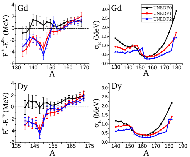
Figure 1: (Color online) Differences between theoretical and experimental binding energies for even-even dysprosium and gadolinium isotopes with error bars representing statistical model error (on the left) and related statistical model error (on the right) as a function of the mass number.

The differences between the theoretical and experimental binding energies for even-even gadolinium and dysprosium isotopes are shown in figure 1. The error bars represent the calculated theoretical standard deviations, and they are also given as a function of the mass number in the graphs on the right. The uncertainties are given for all the calculated binding energies, including also those nuclei for which the experimental binding energy is not currently known. As it can be seen, UNEDF0 gives more consistent results with the measured experimental energies for lighter isotopes, whereas UNEDF1 and UNEDF2 seem to improve their accuracy considerably for heavier isotopes. Most of the theoretical results do not overlap with the experimental values, even when including error bars. Two interesting points can be seen in the graphs on the left: ¹⁴⁶Gd and ¹⁴⁸Dy. Both of these nuclei have neutron number of $N=82$, that is, one of the magic numbers. Here, the theoretical predictions for the binding energies given by UNEDF1 and UNEDF2 are comparatively farther away from the experimental results. However, there is no visible increase in the standard deviation of the binding energy of these two nuclei. This suggests that the increased residual is due to underlying model deficiency, and not due to the parameter optimization procedure.

The calculated standard deviations of binding energies are found to be around 0.5–3.0 MeV, 0.4–1.7 MeV, and 0.3–1.5 MeV for UNEDF0, UNEDF1 and UNEDF2, respectively. Even though the standard deviations have a magnitude of one thousandth of the total binding energy, the theoretical uncertainties are still far larger compared to experimental precision, which can be of the order of few keV’s [30]. However, uncertainties of the UNEDF models have decreased after every model: The obtained standard deviation for UNEDF0 is larger compared to two later parameterizations.

The behavior of uncertainty is relatively smooth and the uncertainty of binding energy grows quickly when going towards neutron rich nuclei. In addition, one can also see that uncertainties grow when going towards the other extreme, namely proton rich nuclei. This is an indication that isovector part of the EDFs is not as well constrained as the isoscalar part.

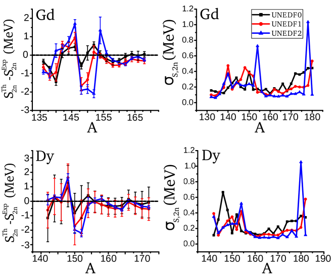
Figure 2: (Color online) Same as figure 1 but for two-neutron separation energy $S_{2n}$.

The residuals of the two-neutron separation energy, $S_{2\rm n}$, are shown in figure 2. The two-neutron separation energies were calculated for even-even Dy and Gd isotopes. Similarly to the previous figure, theoretical errors are marked as error bars in the graphs on the left hand side panels, and also given as a function of the mass number on the right hand side panels. The theoretical statistical error is calculated similarly, through finite differences of $S_{2\rm n}$ values to compute the derivatives. For neutron rich nuclei, all three parameterizations give essentially the same result for $S_{2\rm n}$, within the error bars. Otherwise, the latest UNEDF2 parameterization seems to differ most from the experimental results when compared to previous two parameterizations.

Since $S_{2n}$ is defined as a difference of two binding energies, the partial derivatives are also calculated from energy difference between two nucleus. As a consequence, some of the parameter uncertainties can cancel each other. In particularly, the uncertainty coming from a relatively less constrained isovector part of the EDF is now partly canceled, resulting to more moderate uncertainty in the neutron rich region compared to the uncertainty of binding energy. Similar observation was also done at [9].

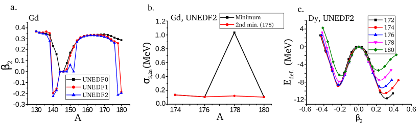
Figure 3: (Color online) Panel a: Deformation parameter $\beta_{2}$ as a function of mass number $A$. Panel b: Calculated statistical error of $\sigma_{S,2n}$ when using either lowest or secondary energy minimum of ¹⁷⁸Gd. Panel c: Deformation energies of five dysprosium isotopes as a function of deformation parameter $\beta_{2}$.

One common feature for all UNEDF models is an existence of a few high peaks in the statistical error of $S_{2n}$. These peaks are located mainly around the same neutron numbers for Gd and Dy isotopes. For instance, the two highest peaks given by UNEDF2 are located at the nuclei ¹⁷⁸Gd and ¹⁸⁰Dy. The explanation for all of the high peaks can be found in a sudden change in deformation. Figure 3, in panel a, shows how deformation parameter $\beta_{2}$ varies with mass number $A$ for Gd. When comparing this to that of $\sigma_{S,2n}$, shown in figure 2, one can notice similarity between uncertainty peaks and large change in the deformation. If there is a significant difference in deformation between two consecutive even-even nuclei, this results to a larger statistical error of two-neutron separation energy.

The relationship between $\sigma_{S,2n}$ and a sudden large change of $\beta_{2}$ can be tested by looking at the secondary local minimum of the deformation energy landscape. For the calculated Gd and Dy nuclei, there usually exists two energy minima, the oblate one and the prolate one, as shown in figure 3, panel c. By picking always the lowest minimum results to large statistical error of $S_{2n}$ when deformation has a large change between two even nucleus. However, if one uses the secondary minimum, in which case the two nuclei appearing in the expression of $S_{2n}$ have similar deformation compared to the each other, one obtains substantially smaller $\sigma_{S,2n}$. In figure 3, panel b, the black line describes the same peak at $A=178$ given by UNEDF2 as in figure 2, calculated with the lowest energy minima. The second (red) line corresponds to case where second minimum of ¹⁷⁸Gd was used, resulting a much smaller $\sigma_{S,2n}$ for ¹⁷⁸Gd. Indeed, a large difference in deformation of involved nuclei seems to give large uncertainty on two-neutron separation energy. A possible explanation is considerably different shell structure between these two nuclei due to deformation. The largest impact on the extremely high peaks in $\sigma_{S,2n}$ given by UNEDF2 is connected to the parameter $C_{1}^{JJ}$, whereas for UNEDF1 the main contributors are $M_{s}^{*}$, both $C^{\rho\Delta J}$ together with $C_{0}^{\rho\Delta\rho}$ and $V_{0}^{n}$ parameters.

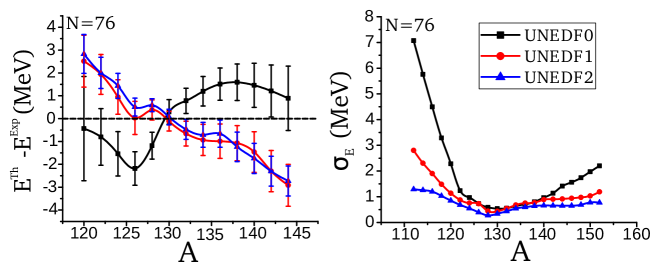
Figure 4: (Color online) Same as figure 1, but for the isotonic chain with the neutron number $N=76$.

The binding energy residuals between theory and experiment for isotonic chain of $N=76$ can be found in figure 4. Only even-even nuclei are studied. The UNEDF1 and UNEDF2 parameterizations give rather similar results, but the binding energy behavior of UNEDF0 parameterization is notably different. Compared to the UNEDF0 optimization procedure, in the optimization of UNEDF1 the same set of 12 EDF parameters were optimized but seven additional data points were included in the database and the center of mass correction was neglected [21]. The other important remark is the fact that even though the trend of UNEDF1 and UNEDF2 models is incorrect – the calculated binding energies for proton rich nuclei are getting further far away from the experimental ones when mass number increases – the uncertainties do not nevertheless become larger.

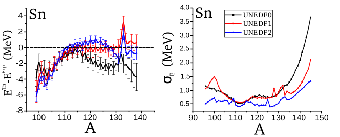
Figure 5: (Color online) Same as figure 1 but for even-even and even-odd Sn isotopes.

We have also considered the statistical error of odd-even nuclei. The binding energy residual for Sn isotopic chain was computed by using all three UNEDF models. The results are shown in figure 5. The odd-even nuclei were calculated by using the quasiparticle blocking procedure with the equal filling approximation [7]. The same blocking configuration, which corresponded the lowest energy with unshifted parameterization, was used for calculation of all partial derivatives. The same set of results for even Sn isotopes, with UNEDF0, was calculated in [9]. The results show that the binding energy residuals of even-even nuclei are relatively greater compared to those of odd nuclei. On this account, the binding energy residuals stagger between the odd and even nuclei. Nevertheless, there are no visible odd-even effects in the standard deviations of binding energy. This can be explained by the lack of time-odd part in the used EDFs.

3.2 Uncertainty of $Q_{2,p}$ and proton matter radius

The standard deviation of proton matter quadrupole moment $Q_{2,p}$ and proton matter root-mean-square (rms) radius $r_{p,rms}$ for all three UNEDF models is shown in figure 6. The scale of $\sigma_{Q2}$ can be read on the left side and the scale of $\sigma_{r}$ on the right side of the figure. As expected, the uncertainty of these two observables behaves similarly and is strongly correlated. High values of uncertainty are located in deformed nuclei next to spherical nuclei, due to soft deformation energy landscape with respect of quadrupole deformation.

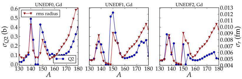
Figure 6: (Color online) The standard deviation of proton quadrupole moment $Q_{2,p}$ and proton rms radius $r_{p,rms}$ for Gd isotopic chain with all three UNEDF models. The scale of $\sigma_{Q2}$ can be read on the left side and the scale of $\sigma_{r}$ on the right side of the figure

Despite the general strong correlation between $\sigma_{r}$ and $\sigma_{Q2}$, with UNEDF1 and UNEDF2, there are a few points of $Q_{2,p}$ which differ from the major trend. The vanishing uncertainty of $Q_{2,p}$ in ¹⁵²Gd is explained by the fact that ¹⁵²Gd is predicted to be spherical by UNEDF2 EDF. This can be seen in figure 3, panel a. The divergent uncertainty of $Q_{2,p}$ in ¹⁸⁰Gd (¹⁷⁸Gd, ¹⁸⁰Gd) in UNEDF1 (UNEDF2) is related to the change of sign in quadrupole moment and deformation parameter $\beta_{2}$ which is shown also in figure 3, panel a. Most of the nuclei are predicted to be prolate by UNEDF1 and UNEDF2, but above-mentioned nuclei are predicted to be oblate, resulting to rapid changes of the statistical uncertainty of $Q_{2,p}$ for Gd isotopic chain. However, ¹⁴⁰Gd and ¹⁴²Gd isotope are also predicted to be oblate by UNEDF1 and UNEDF2 EDFs, but there is no significant effect in the uncertainties given by UNEDF1. There is no oblate-shaped nuclei among the Gd isotopes calculated with UNEDF0 EDF.

In addition to the large uncertainties next to the spherical nuclei, there is also another visible trend in the uncertainties. Similarly like with the uncertainties of the binding energy, when going towards the neutron rich nuclei, the uncertainties of $Q_{2,p}$ and $r_{p,rms}$ increases systematically. The same behavior is also followed with the uncertainties of the neutron matter radius.

3.3 Contributions of the model parameters

One of the goals of present work is to study contributions of the model parameters to the total error budget of binding energy. The most elementary way to represent the contributions of the model parameters to the total uncertainty is by listing component matrix. Here, every single small color square in the matrix represents the value of one particular cross contribution coming from parameters ($x_{i},x_{j}$) to the total sum of equation (9). The component matrices for the binding energy uncertainties of ¹⁵⁴Gd and ¹⁸⁰Gd are shown in figure 7. Some of these components have negative sign, due to a negative partial derivative or a negative covariance matrix element. The total squared standard deviation is always, nevertheless, a positive number. One should also bear in mind that the contribution of a parameter to the standard deviation is visible only if this parameter was included in the sensitivity analysis, as mentioned before.

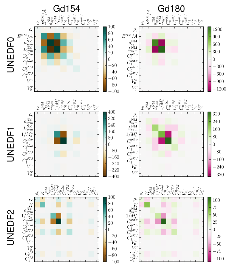
Figure 7: (Color online) Individual contributions of the model parameters ($x_{i},x_{j}$), in the total sum of equation (9), for the uncertainty of binding energy in ¹⁵⁴Gd and ¹⁸⁰Gd isotopes and for all three UNEDF models. The contributions are in units of MeV².

For ¹⁵⁴Gd, which has one of the smallest statistical error of binding energy with all UNEDF parameterizations, the total error budget with UNEDF0 and UNEDF2 EDFs consist of several components. The total error budget with UNEDF1 is simpler, and mainly coming from $1/M_{s}^{*}$ and $C_{0}^{\rho\Delta\rho}$ parameters. On the other hand, the uncertainty budget for the neutron rich nucleus ¹⁸⁰Gd splits into several pieces when going from the oldest parameterization to the latest one. The uncertainty of UNEDF0 is affected by a couple of parameters, mainly by $a^{\rm NM}_{\rm sym}$ and $L^{\rm NM}_{\rm sym}$. The most contributing parameters to the uncertainty of UNEDF1 are $1/M_{s}^{*}$ and $C_{0}^{\rho\Delta\rho}$, whereas in the case of UNEDF2 the $C_{0}^{\rho\Delta\rho}$ parameter have slightly greater contribution. Even though one parameter has slightly greater contribution, the uncertainty of binding energy for neutron rich nuclei is relatively widely spread among the model parameters of UNEDF2.

The component matrix representation shows explicitly how different model parameters contribute to the total error budget pairwise. Unfortunately, this representation requires a lot of space. By considering a summed contribution of one row (or, equivalently, one column) of the component matrix, we can represent the error budget as a stacked histograms for each isotope. We refer this once summed contribution as a row contribution of a parameter $x_{i}$. Here, components of the total error are calculated by summing over one index in equation (9), resulting the total squared standard deviation being then a sum of all row contributions.

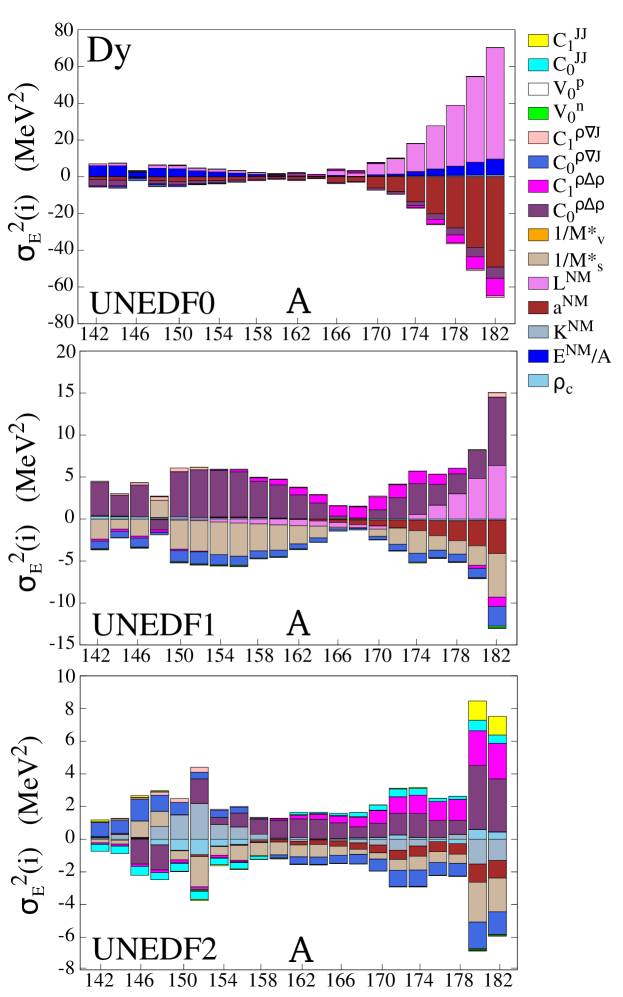
Figure 8: (Color online) Error budget of $\sigma_{E}^{2}$ for even-even Dy isotopes with UNEDF0, UNEDF1 and UNEDF2 EDFs in the row contribution representation. The contribution of a summed up row is indicated with corresponding model parameter name.

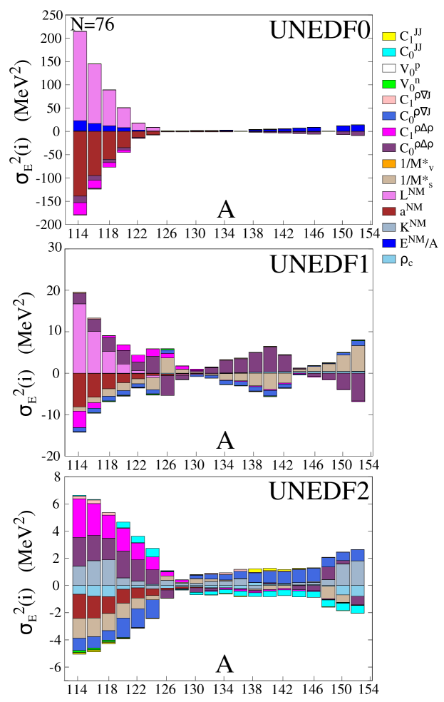
Figure 9: (Color online) Same as figure 8 but for the isotonic chain of $N=76$.

The results for the row contributions are shown in figure 8 for the binding energies of even Dy isotopes and in figure 9 for the binding energies of even $N=76$ isotones. The error budget for UNEDF0 binding energy is mainly composed of only a few contributing rows. For nuclei close to the valley of stability, two dominant sources of uncertainty are the rows $E^{\rm NM}/A$ and $C_{0}^{\rho\Delta\rho}$ parameters, whereas in the neutron rich Dy isotopes the rows of $L_{\rm sym}^{\rm NM}$ and $a_{\rm sym}^{\rm NM}$ dominate. In other words, model parameters related to symmetry energy become more important with neutron rich nuclei. It was found earlier that $L_{\rm sym}^{\rm NM}$ has also a strong impact on the statistical error of neutron root-mean-square radii and neutron skin thickness [9, 29]. The most dominant sources of uncertainty are the same for isotopic and isotonic chains.

Contrary to UNEDF0, the error budget of latter two parameterizations is more split among the various different row contributions in neutron rich nuclei. Generally speaking, the rows connected to $a^{\rm NM}_{\rm sym}$, both $C_{t}^{\rho\Delta\rho}$ parameters, $C_{0}^{\rho\nabla J}$, and $1/M^{*}_{s}$ have a significant impact on the total error budget with UNEDF2. It should be noticed that the correlation between $C_{0}^{\rho\Delta\rho}$ and $1/M^{*}_{s}$ is strong: In principle, if one can reduce the uncertainty on $C_{0}^{\rho\Delta\rho}$, it should also reduce the uncertainty of $1/M^{*}_{s}$. The isovector parameters, for their part, are more difficult to constrain, but they impact on the stability of the functional: For instance $C_{1}^{\rho\Delta\rho}$ is the coupling constant of the gradient term, which has been found to trigger scalar-isovector instabilities [31].

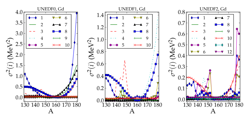
Figure 10: (Color online) The uncertainties of binding energies in the eigenmode formalism. Each curve represents the contribution of one eigenvector. The eigenvectors are different for each UNEDF parameterization, even though symbols and numbering is the same.

Lastly, we represent the uncertainties of binding energies in the eigenmode formalism in figure 10. The eigenvectors are listed in descending order of eigenvalues. The eigenvectors and eigenvalues are not shown here - it is not a laborious task to diagonalize covariance matrices given in references [20, 21, 22]. Basically, a small eigenvalue means that the linear combination of model parameters described by this eigenvector is well constrained. If the eigenvalue is large, the corresponding eigenvector is poorly constrained. The eigenvector representation does not directly tell about the model parameters themselves, but describes how the uncertainty propagates from a certain linear combinations of the model parameters, instead. As we can see, e.g. for neutron rich nuclei, only five eigenvectors of UNEDF0 contribute significantly to the total error budget. The eigenvector having the greatest eigenvalue, and thus being least constrained, has also the biggest contribution to the error budget among the neutron and proton rich nuclei. In the case of UNEDF1, mainly two eigenvectors contribute to the total error budget of a given nucleus, whereas there are 5 significant contributors with UNEDF2 EDF. Interestingly, with UNEDF1, one can see many contributing eigenvectors at deformation transition region around $A=140$ – $152$.

We can also investigate how different model parameters contribute to the uncertainty, in terms of components of one particular eigenvector. For example, with UNEDF0, the first eigenvector has the biggest contribution with neutron rich nuclei. When looking at the individual components of this eigenvector, the main contributing model parameters are $a^{\rm NM}_{\rm sym}$ and $L^{\rm NM}_{\rm sym}$. With the second largest contributing eigenvector, the contribution of $a^{\rm NM}_{\rm sym}$ is the largest one and with third most contributing eigenvector, the parameters $C_{0}^{\rho\Delta\rho}$, $a^{\rm NM}_{\rm sym}$ and $E^{\rm NM}/A$ are the most important ones. With UNEDF1, the uncertainty of binding energy for neutron rich nuclei comes from $a^{\rm NM}_{\rm sym}$, $L^{\rm NM}_{\rm sym}$ and $C_{0}^{\rho\Delta\rho}$ model parameters when considering the most contributing eigenvector, and from $a^{\rm NM}_{\rm sym}$ and $\rho_{c}$ when considering eigenvector having the second largest contribution. On the other hand, with UNEDF2, the contributions are more split among various model parameters. Largest contributing components of two most important eigenvectors consist of several parameters (more than five). The uncertainty coming from the third most contributing eigenvector consists almost entirely of $a^{\rm NM}_{\rm sym}$ and $\rho_{c}$ model parameters.

In the end of this section, we can conclude that three different methods used in this study, namely the component matrix representation, the histogram representation of row contributions, and the eigenmode method, are in support of each other, with each one having their own advantage.

4 Conclusions

In the present work we have calculated statistical errors of the UNEDF models for binding energy, two-neutron separation energy, proton quadrupole moment and proton rms radius by using information about the covariance matrix of the model parameters. The standard deviation has been interpreted as a statistical error. We have also quantified the contributions of each model parameters to the total error budget by using three different methods and checked if there are any visible odd-even effects in the uncertainties of the UNEDF models. We presented our results for the error budget by using the component matrix representation, the row contribution representation, and finally, by using the eigenmode method. We found out that the standard deviation of binding energy grows quickly when going away from the valley of stability towards proton rich or neutron rich nuclei. Similarly, uncertainties of proton quadrupole moment $Q_{2,p}$ and proton rms radius $r_{rms,p}$ increase rapidly among the neutron rich nuclei as a function of mass number. That is to say, the predictive power of UNEDF models becomes weaker when extrapolating further away from known nuclei to experimentally unknown region. For the Sn isotopic chain, even though there exists odd-even staggering in the residuals of binding energies, no visible odd-even effect was seen in the related errors.

The error budget of the UNEDF parameterizations becomes more evenly split among various model parameters with UNEDF1 and UNEDF2 parameterizations in neutron rich nuclei. This can be seen by using any of the three methods mentioned above. The most dominant contributors to the error budget of neutron rich nuclei with UNEDF0 were $L^{\rm NM}_{\rm sym}$ and $a^{\rm NM}_{\rm sym}$ parameters, that is to say, coefficients related to the symmetry energy. In the case of UNEDF1, $L^{\rm NM}_{\rm sym}$ and $a^{\rm NM}_{\rm sym}$ still have a significant contribution and, in addition, the role of $C_{0}^{\rho\Delta\rho}$ and $1/M^{*}_{s}$ becomes important. With UNEDF2, the role of other model parameters becomes even more prominent.

A comparison of the binding energy standard deviations to the residuals seems to point out that the underlying theoretical model is missing some important physics. One clear indication of this is the increase of the binding energy residuals close to the semi-magic nuclei. However, calculated standard deviation does not usually reflect this kind of behavior. Similar observation was also done in [9]. Also, the systematically incorrect trend of UNEDF1 and UNEDF2 with the binding energy residual in the $N=76$ isotonic chain does not appear in theoretical uncertainties, as shown in figure 4.

The trend in the UNEDF statistical errors is such that the calculated standard deviation decreases as more data is included in the optimization procedure. From a statistical point of view, the larger uncertainty of the isovector parameters reflects to the increasing uncertainty when going towards the both isospin extremes. Unfortunately, new data may not always help to reduce uncertainties. A sophisticated parameter optimization within Bayesian framework showed that new data points on nuclear binding energies at neutron rich region were not able provide a better constraint for the UNEDF1 model parameters [16]. On the other hand, data on the neutron skin thickness could potentially help to reduce uncertainties related on isovector model parameters [32].

As was concluded for the UNEDF2 parameterization, the limits of standard Skyrme-EDFs have been reached and novel approaches are called for [22]. Information about the shortcomings and uncertainties of present models will provide valuable input for development of novel EDF models. A comprehensive sensitivity analysis of a novel EDF parameterization is essential when addressing its predictive power.

Appendix A Appendix: Correlation matrices

Table 2: Correlation matrix and standard deviations of the UNEDF0 parameter set [20]. The values are rounded. The units are following: $\rho_{\rm c}$ is in fm^-3; $E^{\rm NM}/A$, $a_{\rm sym}^{\rm NM}$ and $L_{\rm sym}^{\rm NM}$ are in MeV; $C_{t}^{\rho\Delta\rho}$ and $C_{0}^{\rho\nabla J}$ are in MeV fm^-5, and $V_{0}^{n,p}$ are in MeV fm^-3.

	$\rho_{\rm c}$	$E^{\rm NM}/A$	$a_{\rm sym}^{\rm NM}$	$L_{\rm sym}^{\rm NM}$	$C_{0}^{\rho\Delta\rho}$	$C_{1}^{\rho\Delta\rho}$	$V_{0}^{n}$	$V_{0}^{p}$	$C_{0}^{\rho\nabla J}$	$C_{1}^{\rho\nabla J}$
$\rho_{\rm c}$	1.00
$E^{\rm NM}/A$	-0.28	1.00
$a_{\rm sym}^{\rm NM}$	-0.10	-0.88	1.00
$L_{\rm sym}^{\rm NM}$	-0.17	-0.80	0.97	1.00
$C_{0}^{\rho\Delta\rho}$	0.09	0.80	-0.81	-0.74	1.00
$C_{1}^{\rho\Delta\rho}$	0.20	0.35	-0.47	-0.66	0.23	1.00
$V_{0}^{n}$	0.02	0.21	-0.23	-0.25	0.23	0.23	1.00
$V_{0}^{p}$	-0.13	-0.42	0.52	0.56	-0.29	-0.45	-0.14	1.00
$C_{0}^{\rho\nabla J}$	0.37	-0.14	0.02	-0.00	0.44	-0.02	0.09	0.16	1.00
$C_{1}^{\rho\nabla J}$	-0.06	-0.18	0.27	0.33	-0.38	-0.20	-0.01	0.00	-0.37	1.00
$\sigma$	0.001	0.055	3.058	40.037	1.697	56.965	2.105	3.351	3.423	29.460

Table 3: Same as table 2 but for UNEDF1. $L_{\rm sym}^{\rm NM}$ is in units of MeV and $1/M^{*}_{\rm s}$ is unitless.

	$\rho_{\rm c}$	$a_{\rm sym}^{\rm NM}$	$L_{\rm sym}^{\rm NM}$	$1/M^{*}_{\rm s}$	$C_{0}^{\rho\Delta\rho}$	$C_{1}^{\rho\Delta\rho}$	$V_{0}^{n}$	$V_{0}^{p}$	$C_{0}^{\rho\nabla J}$	$C_{1}^{\rho\nabla J}$
$\rho_{\rm c}$	1.00
$a_{\rm sym}^{\rm NM}$	-0.35	1.00
$L^{\rm NM}$	-0.14	0.71	1.00
$1/M^{*}_{\rm s}$	0.32	0.23	0.36	1.00
$C_{0}^{\rho\Delta\rho}$	-0.25	-0.25	-0.35	-0.99	1.00
$C_{1}^{\rho\Delta\rho}$	-0.06	-0.15	-0.77	-0.22	0.19	1.00
$V_{0}^{n}$	-0.32	-0.22	-0.36	-0.99	0.98	0.22	1.00
$V_{0}^{p}$	-0.33	-0.18	-0.29	-0.97	0.97	0.15	0.96	1.00
$C_{0}^{\rho\nabla J}$	-0.14	-0.20	-0.32	-0.86	0.91	0.22	0.85	0.84	1.00
$C_{1}^{\rho\nabla J}$	0.05	-0.17	-0.13	-0.10	0.07	0.21	0.10	0.07	-0.03	1.00
$\sigma$	0.0004	0.604	13.136	0.123	5.361	52.169	18.561	13.049	5.048	23.147

Table 4: Same as table 2 but for UNEDF2. The parameters $C_{1}^{\rho\nabla J}$ are in units of MeV fm^-3.

	$\rho_{\rm c}$	$K_{\rm sym}^{\rm NM}$	$a_{\rm sym}^{\rm NM}$	$1/M^{*}_{\rm s}$	$C_{0}^{\rho\Delta\rho}$	$C_{1}^{\rho\Delta\rho}$	$V_{0}^{n}$	$V_{0}^{p}$	$C_{0}^{\rho\nabla J}$	$C_{1}^{\rho\nabla J}$	$C_{0}^{JJ}$	$C_{1}^{JJ}$
$\rho_{\rm c}$	1.00
$K_{\rm sym}^{\rm NM}$	-0.97	1.00
$a_{\rm sym}^{\rm NM}$	-0.07	-0.03	1.00
$1/M^{*}_{\rm s}$	0.08	-0.05	-0.24	1.00
$C_{0}^{\rho\Delta\rho}$	-0.43	0.43	0.22	-0.89	1.00
$C_{1}^{\rho\Delta\rho}$	-0.42	0.37	0.83	-0.17	0.31	1.00
$V_{0}^{n}$	-0.06	0.02	0.27	-0.96	0.85	0.17	1.00
$V_{0}^{p}$	-0.09	0.05	0.21	-0.89	0.80	0.14	0.86	1.00
$C_{0}^{\rho\nabla J}$	-0.51	0.50	0.34	-0.40	0.68	0.55	0.36	0.34	1.00
$C_{1}^{\rho\nabla J}$	-0.31	0.29	-0.19	-0.00	0.04	0.18	-0.07	-0.02	0.14	1.00
$C_{0}^{JJ}$	0.56	-0.55	-0.26	0.05	-0.35	-0.53	-0.02	-0.02	-0.88	-0.35	1.00
$C_{1}^{JJ}$	0.36	-0.35	0.13	-0.23	0.16	-0.14	0.29	0.25	-0.02	-0.57	0.29	1.00
$\sigma$	0.001	10.119	0.321	0.052	2.689	24.322	8.353	6.792	5.841	15.479	16.481	17.798

Appendix B Appendix: Values of the parameters and used finite differences

Table 5: Rounded values $x_{i}$ for each UNEDF parameterization and the corresponding used finite differences $\Delta x_{i}$ used in the derivatives. The units are the same as in tables 2, 3 and 4.

	UNEDF0		UNEDF1		UNEDF2
parameter	$x_{i}$	$\Delta x_{i}$	$x_{i}$	$\Delta x_{i}$	$x_{i}$	$\Delta x_{i}$
$\rho_{c}$	0.161	0.004	0.159	0.004	0.156	0.004
$E_{sym}^{NM}/A$	-16.056	0.02
$K_{sym}^{NM}$					239.930	2.0
$a_{sym}^{NM}$	30.543	0.1	28.987	0.2	29.131	0.2
$L_{sym}^{NM}$	45.080	0.4	40.005	0.4
$1/M^{*}_{s}$			0.992	0.012	1.074	0.012
$C_{0}^{\rho\Delta\rho}$	-55.261	0.6	-45.135	0.6	-46.831	0.6
$C_{1}^{\rho\Delta\rho}$	-55.623	2.0	-145.382	2.0	-113.164	2.0
$V_{0}^{n}$	-170.374	2.0	-186.065	2.0	-208.889	2.0
$V_{0}^{p}$	-199.202	2.0	-206.580	2.0	-230.330	2.0
$C_{0}^{\rho\nabla J}$	-79.531	0.7	-74.026	0.7	-64.308	0.7
$C_{1}^{\rho\nabla J}$	45.630	1.5	-35.658	1.5	-38.650	1.5
$C_{0}^{JJ}$					-54.433	2.0
$C_{1}^{JJ}$					-65.903	4.0

References

References

- [1] Bender M, Heenen P-H, and Reinhard P-G. Rev. Mod. Phys., 75:121, 2003.
- [2] Erler J, Birge N, Kortelainen M, Nazarewicz W, Olsen E, Perhac A, and Stoitsov M. Nature, 486:509, 2012.
- [3] Dutra M, Lourenço O, Sá Martins J S, Delfino A, Stone J R, and Stevenson P D. Phys. Rev. C, 85:035201, 2012.
- [4] Carlsson B G, Dobaczewski J, and Kortelainen M. Phys. Rev. C, 78:044326, 2008.
- [5] Kortelainen M, Dobaczewski J, Mizuyama K, and Toivanen J. Phys. Rev. C, 77:064307, 2008.
- [6] Nazarewicz W. J. Phys. G: Nucl. Part. Phys., 43:044002, 2016.
- [7] Schunck N, Dobaczewski J, McDonnell J, Moré J, Nazarewicz W, Sarich J, and Stoitsov M V. Phys. Rev. C, 81:024316, 2010.
- [8] Dobaczewski J, Nazarewicz W, and Reinhard P-G. J. Phys. G: Nucl. Part. Phys., 41:074001, 2014.
- [9] Gao Y, Dobaczewski J, Kortelainen M, Toivanen J, and Tarpanov D. Phys. Rev. C, 87:034324, 2013.
- [10] Schunck N, McDonnell J D, Sarich J, Wild S M, and Higdon D. J. Phys. G: Nucl. Part. Phys., 42:034024, 2015.
- [11] Rios A and Roca Maza X. J. Phys. G: Nucl. Part. Phys., 42:034005, 2015.
- [12] Nikšić T, Paar N, Reinhard P-G, and Vretenar D. J. Phys. G: Nucl. Part. Phys., 42:034008, 2015.
- [13] Kortelainen M. J. Phys. G: Nucl. Part. Phys., 42:034021, 2015.
- [14] Ekström A, Carlsson B D, Wendt K A, Forssén C, Hjorth-Jensen M, Machleidt R, and Wild S M. J. Phys. G: Nucl. Part. Phys., 42:034003, 2015.
- [15] Lähde T A, Epelbaum E, Krebs H, Lee D, Meißner U-G, and Rupak G. J. Phys. G: Nucl. Part. Phys., 42:034012, 2015.
- [16] McDonnell J D, Schunck N, Higdon D, Sarich J, Wild S M, and Nazarewicz W. Phys. Rev. Lett., 114:122501, 2015.
- [17] Higdon D, McDonnell J D, Schunck N, Sarich J, and Wild S M. J. Phys. G: Nucl. Part. Phys., 42:034009, 2015.
- [18] Graczyk K M and Juszczak C. J. Phys. G: Nucl. Part. Phys., 42:034019, 2015.
- [19] Wesolowski S, Klco N, Furnstahl R J, Phillips D R, and Thapaliya A. J. Phys. G: Nucl. Part. Phys., 43:074001, 2016.
- [20] Kortelainen M, Lesinski T, Moré J, Nazarewicz W, Sarich J, Schunck N, Stoitsov M V, and Wild S. Phys. Rev. C, 82:024313, 2010.
- [21] Kortelainen M, McDonnell J, Nazarewicz W, Reinhard P-G, Sarich J, Schunck N, Stoitsov M V, and Wild S M. Phys. Rev. C, 85:024304, 2012.
- [22] Kortelainen M, McDonnell J, Nazarewicz W, Olsen E, Reinhard P-G, Sarich J, Schunck N, Wild S M, Davesne D, Erler J, and Pastore A. Phys. Rev. C, 89:054314, 2014.
- [23] Ring P and Schuck P. The Nuclear Many-Body Problem. Springer, 2004.
- [24] Chabanat E, Bonche P, Haensel P, Meyer J, and Schaeffer R. Nuclear Physics A, 627:710, 1997.
- [25] Audi G, Wang M, Wapstra A H, Kondev F G, MacCormick M, Xu X, and Pfeiffer B. Chinese Physics C, 36:1287, 2012.
- [26] Fattoyev F J and Piekarewicz J. Phys. Rev. C, 84:064302, 2011.
- [27] Stoitsov M V, Dobaczewski J, Nazarewicz W, and Ring P. Comput. Phys. Commun., 167:43, 2005.
- [28] Stoitsov M V, Schunck N, Kortelainen M, Michel N, Nam H, Olsen E, Sarich J, and Wild S. Comp. Phys. Comm., 184:1592, 2013.
- [29] Kortelainen M, Erler J, Nazarewicz W, Birge N, Gao Y, and Olsen E. Phys. Rev. C, 88:031305, 2013.
- [30] Kankainen A, Äystö J, and Jokinen A. J. Phys. G: Nucl. Part. Phys., 39:093101, 2012.
- [31] Hellemans V, Pastore A, Duguet T, Bennaceur K, Davesne D, Meyer J, Bender M, and Heenen P-H. Phys. Rev. C, 88:064323, 2013.
- [32] Reinhard P-G and Nazarewicz W. Phys. Rev. C, 81:051303, 2010.