Ordinal Common-sense Inference

Abstract

Humans have the capacity to draw common-sense inferences from natural language: various things that are likely but not certain to hold based on established discourse, and are rarely stated explicitly. We propose an evaluation of automated common-sense inference based on an extension of recognizing textual entailment: predicting ordinal human responses on the subjective likelihood of an inference holding in a given context. We describe a framework for extracting common-sense knowledge from corpora, which is then used to construct a dataset for this ordinal entailment task. We train a neural sequence-to-sequence model on this dataset, which we use to score and generate possible inferences. Further, we annotate subsets of previously established datasets via our ordinal annotation protocol in order to then analyze the distinctions between these and what we have constructed.

1 Introduction

We use words to talk about the world. Therefore, to understand what words mean, we must have a prior explication of how we view the world. – ?)

Researchers in Artificial Intelligence and (Computational) Linguistics have long-cited the requirement of common-sense knowledge in language understanding. This knowledge is viewed as a key component in filling in the gaps between the telegraphic style of natural language statements: we are able to convey considerable information in a relatively sparse channel, presumably owing to a partially shared model at the start of any discourse.

Sam bought a new clock $\leadsto$ The clock runs

Dave found an axe in his garage $\leadsto$ A car is parked in the garage

Tom was accidentally shot by his teammate in the army $\leadsto$ The teammate dies

Two friends were in a heated game of checkers $\leadsto$ A person shoots the checkers

My friends and I decided to go swimming in the ocean $\leadsto$ The ocean is carbonated

Figure 1: Examples of common-sense inference ranging from very likely, likely, plausible, technically possible, to impossible.

Common-sense inference – inferences based on common-sense knowledge – is possibilistic: things everyone more or less would expect to hold in a given context, but without the necessary strength of logical entailment. Because natural language corpora exhibit human reporting bias [Gordon and Van Durme (2013], systems that derive knowledge exclusively from such corpora may be more accurately considered models of language, rather than of the world [Rudinger et al. (2015]. Facts such as “A person walking into a room is very likely to be blinking and breathing” are usually unstated in text, so their real-world likelihoods do not align to language model probabilities. We would like to have systems capable of, e.g., reading a sentence that describes a real-world situation and inferring how likely other statements about that situation are to hold true in the real world. This capability is subtly but crucially distinct from the ability to predict other sentences reported in the same text, as a language model may be trained to do.

We therefore propose a model of knowledge acquisition based on first deriving possibilistic statements from text: as the relative frequency of these statements suffers the mentioned reporting bias, we then follow up with human annotation of derived examples. Since we initially are uncertain about the real-world likelihood of the derived common-sense knowledge holding in any particular context, we pair it with various grounded context and present to humans for their own assessment. As these examples vary in assessed plausibility, we propose the task of ordinal common-sense inference, which embraces a wider set of natural conclusions arising from language comprehension (see Fig 1).

In what follows, we describe prior efforts in common-sense and textual inference (§2). We then state our position on how ordinal common-sense inference should be defined (§3), and detail our own framework for large-scale extraction and abstraction, along with a crowdsourcing protocol for assessment (§4). This includes a novel neural model for forward generation of textual inference statements. Together these methods are applied to contexts derived from various prior textual inference resources, resulting in the JHU Ordinal Common-sense Inference (JOCI) corpus, a large collection of diverse common-sense inference examples, judged to hold with varying levels of subjective likelihood (§5). We provide baseline results (§6) for prediction on the JOCI corpus.

2 Background

Mining Common Sense

Building large collections of common-sense knowledge can be done manually via professionals [Hobbs and Navarretta (1993], but at considerable cost in terms of time and expense [Miller (1995, Lenat (1995, Baker et al. (1998, Friedland et al. (2004]. Efforts have pursued volunteers [Singh (2002, Havasi et al. (2007] and games with a purpose [Chklovski (2003], but are still left fully reliant on human labor. Many have pursued automating the process, such as in expanding lexical hierarchies [Hearst (1992, Snow et al. (2006], constructing inference patterns [Lin and Pantel (2001, Berant et al. (2011], reading reference materials [Richardson et al. (1998, Suchanek et al. (2007], mining search engine query logs [Paşca and Van Durme (2007], and most relevant here: abstracting from instance-level predications discovered in descriptive texts [Schubert (2002, Liakata and Pulman (2002, Clark et al. (2003, Banko and Etzioni (2007]. In this article we are concerned with knowledge mining for purposes of seeding a text generation process (constructing common-sense inference examples).

Common-sense Tasks

Many textual inference tasks have been designed to require some degree of common-sense knowledge, e.g., the Winograd Schema Challenge discussed by ?). The data for these tasks are either smaller, carefully constructed evaluation sets by professionals, following efforts like the FraCaS test suite [Cooper et al. (1996], or they rely on crowdsourced elicitation [Bowman et al. (2015]. Crowdsourcing is scalable, but elicitation protocols can lead to biased responses unlikely to contain a wide range of possible common-sense inferences: humans can generally agree on the plausibility of a wide range of possible inference pairs, but they are not likely to generate them from an initial prompt.

The construction of SICK (Sentences Involving Compositional Knowledge) made use of existing paraphrastic sentence pairs (descriptions by different people of the same image), which were modified through a series of rule-based transformations then judged by humans [Marelli et al. (2014]. As with SICK, we rely on humans only for judging provided examples, rather than elicitation of text. Unlike SICK, our generation is based on a process targeted specifically at common sense (see §4.1.1).

Plausibility

Researchers in psycholinguistics have explored a notion of plausibility in human sentence processing, where, for instance, arguments to predicates are intuitively more or less “plausible” as fillers to different thematic roles, as reflected in human reading times. For example, ?) looked at manipulations such as:

(a) The boss hired by the corporation was perfect for the job.

(b) The applicant hired by the corporation was perfect for the job.

where the plausibility of a boss being the agent – as compared to patient – of the predicate hired might be measured by looking at delays in reading time in the words following the predicate; this measurement is then contrasted with the timing observed in the same positions in (b).

Rather than measuring according to predictions such as human reading times, here we ask annotators explicitly to judge plausibility on a 5-point ordinal scale (See §3). Further, our effort might be described in this setting as conditional plausibility, where plausibility judgments for a given sentence are expected to be dependent on preceding context. Further exploration of conditional plausibility is an interesting avenue of potential future work, perhaps through the measurement of human reading times when using prompts derived from our ordinal common-sense inference examples. Computational modeling of (unconditional) semantic plausibility has been explored by those such as ?), ?) and ?).

Textual Entailment

A multi-year source of textual inference examples were generated under the Recognizing Textual Entailment (RTE) Challenges, introduced by ?):

We say that T entails H if, typically, a human reading T would infer that H is most likely true. This somewhat informal definition is based on (and assumes) common human understanding of language as well as common background knowledge.

This definition strayed from the more strict notion of entailment as used by linguistic semanticists, such as those involved with FraCaS. While ?) extended binary RTE with an “unknown” category, the entailment community has primarily focussed on issues such as paraphrase and monotonicity, such as captured by the Natural Logic implementation of ?).

Language understanding in context is not only understanding the entailments of a sentence, but also the plausible inferences of the sentence, i.e. the new posterior on the world after reading the sentence. A new sentence in a discourse is almost never entailed by another sentence in the discourse, because such a sentence would add no new information. In order to successfully process a discourse, there needs to be some understanding of what new information can be possibly or plausibly added to the discourse. Collecting sentence pairs with ordinal entailment connections is potentially useful for improving and testing these language understanding capabilities that would be needed by algorithms for applications like storytelling.

?) and ?) treated textual entailment as probabilistic logical inference in Markov Logic Networks [Richardson and Domingos (2006]. But the notion of probability in their entailment task has a subtle distinction from our problem of common-sense inference. The probability of being an entailment given by a probabilistic model trained for a binary classification (being an entailment or not), is not necessarily the same as the likelihood of an inference being true. For example:

T: A person flips a coin.

H: That flip comes up heads.

No human reading $T$ should infer that $H$ is true. A model trained to make ordinal predictions should say: “plausible, with probability 1.0”, whereas a model trained to make binary entailed/not-entailed predictions should say: “not entailed, with probability 1.0”. The following example exhibits the same property:

T: An animal eats food.

H: A person eats food.

Again, with high confidence, $H$ is plausible; and, with high confidence, it is also not entailed.

Non-entailing Inference

Of the various non-“entailment” textual inference tasks, a few are most salient here. ?) piloted a Textual Similarity evaluation which has been refined in subsequent years: systems produce scalar values corresponding to predictions of how similar the meaning is between two provided sentences. E.g., the following pair from SICK was judged very similar (4.2 out of 5), while also being a contradiction: There is no biker jumping in the air and A lone biker is jumping in the air. The ordinal approach we advocate for relies on a graded notion, like textual similarity.

The Choice of Plausible Alternative (COPA) task [Roemmele et al. (2011] was a reaction to RTE, similarly motivated to probe a system’s ability to understand inferences that are not strictly entailed: a single context was provided, with two alternative inferences, and a system had to judge which was more plausible. The COPA dataset was manually elicited, and is not large: we discuss this data further in §5.

The Narrative Cloze task [Chambers and Jurafsky (2008] requires a system to score candidate inferences as to how likely they are to appear in a document that also included the provided context. Many such inferences are then not strictly entailed by the context. Further, the cloze task gives the benefit of being able to generate very large numbers of examples automatically by simply occluding parts of existing documents and asking a system to predict what is missing. The LAMBADA dataset [Paperno et al. (2016] is akin to our strategy for automatic generation followed by human filtering, but for cloze examples. As our concern is with inferences that are often true but never stated in a document, this approach is not viable here. The ROCStories corpus [Mostafazadeh et al. (2016] elicited a more “plausible” collection of documents in order to retain the narrative cloze in the context of common-sense inference. The ROCStories corpus can be viewed as an extension of the idea behind the COPA corpus, done at a larger scale with crowdsourcing, and with multi-sentence contexts; we consider this dataset in §5.

Alongside the narrative cloze, ?) made use of a 5-point Likert scale (very likely to very unlikely) as a secondary evaluation of various script induction techniques. While they were concerned with measuring their ability to generate very likely inferences, here we are interested in generating a wide swath of inference candidates, including those that are impossible.

3 Ordinal Common-sense Inference

Our goal is a system that can perform speculative, common-sense inference as part of understanding language. Based on the observed shortfalls of prior work, we propose the notion of Ordinal Common-sense Inference (OCI). OCI embraces the notion of ?), in that we are concerned with human judgements of epistemic modality.

As agreed by many linguists, modality in natural language is a continuous category, but speakers are able to map areas of this axis into discrete values [Lyons (1977, Horn (1989, de Haan (1997] – ?)

According to ?), there are two scales of epistemic modality which differ in polarity (positive vs. negative polarity): $\langle$certain, likely, possible$\rangle$ and $\langle$impossible, unlikely, uncertain$\rangle$. The Square of Opposition (SO) (Footnote 11) illustrates the logical relations holding between values in the two scales. Based on their logical relations, we can make a set of exhaustive epistemic modals: $\langle$very likely, likely, possible, impossible$\rangle$, where $\langle$very likely, likely, possible$\rangle$ lie on a single, positive Horn scale, and impossible, a complementary concept from the corresponding negative Horn scale, completes the set. In this paper, we further replace the value possible by the more fine-grained values (technically possible and plausible). This results in a 5-point scale of likelihood: $\langle$very likely, likely, plausible, technically possible, impossible$\rangle$. The OCI task definition directly embraces subjective likelihood on such an ordinal scale. Humans are presented with a context $\mathcal{C}$ and asked whether a provided hypothesis $\mathcal{H}$ is very likely, likely, plausible, technically possible, or impossible. Furthermore, an important part of this process is the generation of $\mathcal{H}$ by automatic methods, which seeks to avoid the elicitation bias of many prior works.

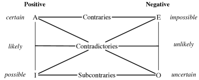
Figure 2: SO for epistemic modals [Saurí and Pustejovsky (2009].

4 Framework for collecting OCI corpus

We now describe our framework for collecting ordinal common-sense inference examples. It is natural to collect this data in two stages. In the first stage (§4.1), we automatically generate inference candidates given some context. We propose two broad approaches using either general world knowledge or neural methods. In the second stage (§4.2), we annotate these candidates with ordinal labels.

4.1 Generation of Common-sense Inference Candidates

4.1.1 Generation based on World Knowledge

Our motivation for this approach was first introduced by ?):

There is a largely untapped source of general knowledge in texts, lying at a level beneath the explicit assertional content. This knowledge consists of relationships implied to be possible in the world, or, under certain conditions, implied to be normal or commonplace in the world.

Following ?) and ?), we define an approach for abstracting over explicit assertions derived from corpora, leading to a large-scale collection of general possibilistic statements. As shown in Fig 3, this approach generates common-sense inference candidates in four steps: (a) extracting propositions with predicate-argument structures from texts, (b) abstracting over propositions to generate templates for concepts, (c) deriving properties of concepts via different strategies, and (d) generating possibilistic hypotheses from contexts.

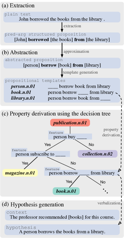
Figure 3: Generating common-sense inferences based on general world knowledge.

(a) Extracting propositions: First we extract a large set of propositions with predicate-argument structures from noun phrases and clauses, under which general world presumptions often lie. To achieve this goal, we use PredPatt [White et al. (2016], which defines a framework of interpretable, language-neutral predicate-argument extraction patterns from Universal Dependencies [de Marneffe et al. (2014]. Fig 3 (a) shows an example extraction.

We use the Gigaword corpus [Parker et al. (2011] for extracting propositions as it is a comprehensive text archive. There exists a version containing automatically generated syntactic annotation [Ferraro et al. (2014], which bootstraps large-scale knowledge extraction. We use PyStanfordDependencies to convert constituency parses to depedency parses, from which we extract structured propositions.

(b) Abstracting propositions: In this step, we abstract the propositions into a more general form. This involves lemmatization, stripping inessential modifiers and conjuncts, and replacing specific arguments with generic types. This method of abstraction often yields general presumptions about the world. To reduce noise from predicate-argument extraction, we only keep 1-place and 2-place predicates after abstraction.

We further generalize individual arguments to concepts by attaching semantic-class labels to them. Here we choose WordNet [Miller (1995] noun synsets as the semantic-class set. When selecting the correct sense for an argument, we adopt a fast and relatively accurate method: always taking the first sense which is usually the most commonly used sense [Suchanek et al. (2007, Pasca (2008]. By doing so, we attach 84 million abstracted propositions with senses, covering 43.7% (35,811/81,861) of WordNet noun senses.

Each of these WordNet senses, then, is associated with a set of abstracted propositions. The abstracted propositions are turned into templates by replacing the sense’s corresponding argument with a placeholder, similar to ?) (see Fig 3 (b)). We remove any template associated with a sense if it occurs less than two times for that sense, leaving 38 million unique templates.

(c) Deriving properties via WordNet: At this step, we want to associate with each WordNet sense a set of possible properties. We employ three strategies.

The first strategy is to use a decision tree to pick out highly discriminative properties for each WordNet sense. Specifically, for each set of co-hyponyms, we train a decision tree using the associated templates as features. For example, in Fig 3 (c), we train a decision tree over the co-hyponyms of publication.n.01. Then the template “person subscribe to ____” would be selected as a property of magazine.n.01, and the template “person borrow ____ from library” for book.n.01. The second strategy selects the most frequent templates associated with each sense as properties of that sense. The third strategy uses WordNet ISA relations to derive new properties of senses. E.g. for the sense book.n.01 and its hypernym publication.n.01, we generate a property “____ be publication”.

(d) Generating hypotheses: As shown in Fig 3 (d), given a discourse context [Tanenhaus and Seidenberg (1980], we first extract an argument of the context, then select the derived properties for the argument. Since we don’t assume any specific sense for the argument, these properties could come from any of its candidate senses. We generate hypotheses by replacing the placeholder in the selected properties with the argument, and verbalizing the properties.

4.1.2 Generation via Neural Methods

In addition to the knowledge-based methods described above, we also adapt a neural sequence-to-sequence model [Vinyals et al. (2015, Bahdanau et al. (2014] to generate inference candidates given contexts. The model is trained on sentence pairs labeled “entailment” from the SNLI corpus [Bowman et al. (2015] (train). Here, the SNLI “premise” is the input (context $\mathcal{C}$), and the SNLI “hypothesis” is the output (hypothesis $\mathcal{H}$).

We employ two different strategies for forward generation of inference candidates given any context. The sentence-prompt strategy uses the entire sentence in the context as an input, and generates output using greedy decoding. The word-prompt strategy differs by using only a single word from the context as input. This word is chosen in the same fashion as the step (d) in generation based on world knowledge, i.e. an argument of the context. The second approach is motivated by our hypothesis that providing only a single word context will force the model to generate a hypothesis that generalizes over the many contexts in which that word was seen, resulting in more common-sense-like hypotheses, as in Fig 4. We later present the full context and decoded hypotheses to crowdsource workers for annotation.

dustpan $\leadsto$ a person is cleaning.

a boy in blue and white shorts is sweeping with a broom and dustpan. $\leadsto$ a young man is holding a broom.

Figure 4: Examples of sequence-to-sequence hypothesis generation from single-word and full-sentence inputs.

Neural Sequence-to-Sequence Model

Neural sequence-to-sequence models learn to map variable-length input sequences to variable-length output sequences, as a conditional probability of output given input. For our purposes, we want to learn the conditional probability of an hypothesis sentence, $\mathcal{H}$, given a context sentence, $\mathcal{C}$, i.e., $P(\mathcal{H}|\mathcal{C})$.

The sequence-to-sequence architecture consists of two components: an encoder and a decoder. The encoder is a recurrent neural network (RNN) iterating over input tokens (i.e., words in $\mathcal{C}$), and the decoder is another RNN iterating over output tokens (words in $\mathcal{H}$). The final state of the encoder, $\textbf{h}_{\mathcal{C}}$, is passed to the decoder as its initial state. We use a three-layer stacked LSTM (state size 512) for both the encoder and decoder RNN cells, with independent parameters for each. We use the LSTM formulation of ?) as summarized in ?).

The network computes $P(\mathcal{H}|\mathcal{C})$:

$$P(\mathcal{H}|\mathcal{C})=\prod\limits_{t=1}^{\text{len}(\mathcal{H})}p(w_{t}|w_{<t},\mathcal{C})$$ (1)

where $w_{t}$ are the words in $\mathcal{H}$. At each time step, $t$, the successive conditional probability is computed from the LSTM’s current hidden state:

$$p(w_{t}|w_{<t},\mathcal{C})\propto\text{exp}(\textbf{v}_{w_{t}}\cdot\textbf{h}_{t})$$ (2)

where $\textbf{v}_{w_{t}}$ is the embedding of word $w_{t}$ from its corresponding row in the output vocabulary matrix, $V$ (a learnable parameter of the network), and $\textbf{h}_{t}$ is the hidden state of the decoder RNN at time $t$. In our implementation, we set the vocabulary to be all words that appear in the training data at least twice, resulting in a vocabulary of size 24,322.

This model also makes use of an attention mechanism. An attention vector, $attn_{t}$, is concatenated with the LSTM hidden state at time $t$ to form the hidden state, $\textbf{h}_{t}$, from which output probabilities are computed (Eqn. 2). This attention vector is a weighted average of the hidden states of the encoder, $h_{1\leq i\leq\text{len}(\mathcal{C})}$:

$$u_{i}^{t} =v^{T}\text{tanh}(W_{1}h_{i}+W_{2}h_{t})$$ (3)

$$a_{i}^{t} =\text{softmax}(u_{i}^{t})$$

$$attn_{t} =\sum\limits_{i=1}^{\text{len}(\mathcal{C})}a_{i}^{t}h_{i}$$

where vector $v$ and matrices $W_{1}$, $W_{2}$ are parameters.

The network is trained via backpropagation on the cross-entropy loss of the observed sequences in training. A sampled softmax is used to compute the loss during training, while a full softmax is used after training to score unseen $(\mathcal{C},\mathcal{H})$ pairs, or generate an $\mathcal{H}$ given a $\mathcal{C}$. Generation is performed via beam search with a beam size of 1; the highest probability word is decoded at each time step and fed as input to the decoder at the next time step until an end-of-sequence token is decoded.

4.2 Ordinal Label Annotation

In this stage, we turn to human efforts to annotate common-sense inference candidates with ordinal labels. The annotator is given a context, and then is asked to assess the likelihood of the hypotheses being true. These context-hypothesis pairs are annotated with one of the five labels: very likely, likely, plausible, technically possible, and impossible, corresponding to the ordinal values of $\{$5,4,3,2,1$\}$ respectively.

In the case that the hypotheses in the inference candidates do not make sense, or have grammatical errors, judges can provide an additional label, NA, so that we can filter these candidates in post-processing. The combination of generation of common-sense inference candidates with human filtering seeks to avoid the problem of elicitation bias.

5 JOCI Corpus

We now describe in depth how we created the JHU Ordinal Common-sense Inference (JOCI) corpus. The main part of the corpus consists of contexts chosen from SNLI [Bowman et al. (2015] and ROCStories [Mostafazadeh et al. (2016], paired with hypotheses generated via methods described in §4.1. These pairs are then annotated with ordinal labels using crowdsourcing (§4.2). We also include context-hypothesis pairs directly taken from SNLI and other corpora (e.g., as premise-hypothesis pairs), and re-annotate them with ordinal labels.

5.1 Data sources for Context-Hypothesis Pairs

In order to compare with existing inference corpora, we choose contexts from two resources: (1) the first sentence in the sentence pairs of the SNLI corpus which are captions from the Flickr30k corpus [Young et al. (2014], and (2) the first sentence in the stories of the ROCStories corpus.

We then collect candidates of automatically generated common-sense inferences (AGCI) against these contexts. Specifically, in the SNLI train set, there are over 150K different first sentences, involving 7,414 different arguments according to predicate-argument extraction. We randomly choose 4,600 arguments. For each argument, we sample one first sentence that has the argument, and collect candidates of AGCI against this as context. We also do the same generation for the SNLI development set and test set. We also collect candidates of AGCI against randomly sampled first sentences in the ROCStories corpus. Collectively, these pairs and their ordinal labels (to be described in § 5.2) make up the main part of the JOCI corpus. The statistics of this subset are shown in Table 1 (first five rows).

For comprehensiveness, we also produced ordinal labels on $(\mathcal{C},\mathcal{H})$ pairs directly drawn from existing corpora. For SNLI, we randomly select 1000 contexts (premises) from the SNLI train set. Then, the corresponding hypothesis is one of the entailment, neutral, or contradiction hypotheses taken from SNLI. For ROCStories, we defined $\mathcal{C}$ as the first sentence of the story, and $\mathcal{H}$ as the second or third sentence. For COPA, $(\mathcal{C},\mathcal{H})$ corresponds to premise-effect. The statistics are shown in the bottom rows of Table 1.

Subset Name	# pairs	Context Source	Hypothesis Source
AGCI against SNLI/ROCStories	22,086	SNLI-train	AGCI-wk
	2,456	SNLI-dev	AGCI-wk
	2,362	SNLI-test	AGCI-wk
	5,002	ROCStories	AGCI-wk
	1,211	SNLI-train	AGCI-nn
SNLI	993	SNLI-train	SNLI-entailment
	988	SNLI-train	SNLI-neutral
	995	SNLI-train	SNLI-contradiction
ROCStories	1,000	ROCStories-1st	ROCStories-2nd
	1,000	ROCStories-1st	ROCStories-3rd
COPA	1,000	COPA-premise	COPA-effect
Total	39,093	-	-

Table 1: JOCI corpus statistics, where each subset consists of different sources for context-and-hypothesis pairs, each annotated with common-sense ordinal labels. AGCI-wk represents candidates generated based on world knowledge. AGCI-nn represents candidates generated via neural methods.

5.2 Crowdsourced Ordinal Label Annotation

We use Amazon Mechanical Turk to annotate the hypotheses with ordinal labels. In each HIT (Human Intelligence Task), a worker is presented with one context and one or two hypotheses, as shown in Fig 5. First, the annotator sees an “Initial Sentence” (context), e.g. “John’s goal was to learn how to draw well.”, and is then asked about the plausibility of the hypothesis, e.g. “A person accomplishes the goal”. In particular, we ask the annotator how plausible the hypothesis is true during or shortly after, because without this constraint, most sentences are technically plausible in some imaginary world.

If the hypothesis does not make sense, the workers can check the box under the question and skip the ordinal annotation. In the annotation, about 25% of hypotheses are marked as not making sense, and are removed from our data.

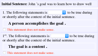
Figure 5: The annotation interface, with a drop-down list provides ordinal labels to select.

M.	Labels	Context	Hypothesis
5	[5,5,5]	John was excited to go to the fair	The fair opens .
4	[4,4,3]	Today my water heater broke	A person looks for a heater .
3	[3,3,4]	John ’s goal was to learn how to draw well	A person accomplishes the goal .
2	[2,2,2]	Kelly was playing a soccer match for her University	The University is dismantled .
1	[1,1,1]	A brown-haired lady dressed all in blue denim sits in a group of pigeons .	People are made of the denim .
5	[5,5,4]	Two females are playing rugby on a field, one with a blue uniform and one with a white uniform .	Two females are play sports outside .
4	[4,4,3]	A group of people have an outside cookout .	People are having conversations .
3	[3,3,3]	Two dogs fighting, one is black, the other beige .	The dogs are playing .
2	[2,2,3]	A bare headed man wearing a dark blue cassock, sandals, and dark blue socks mounts the stone steps leading into a weathered old building	A man is in the middle of home building .
1	[1,1,1]	A skydiver hangs from the undercarriage of an airplane or some sort of air gliding device	A camera is using an object .

Table 2: Examples of context-and-hypothesis pairs with ordinal judgements and Median value.
(The upper 5 rows are samples from AGCI-wk. The lower 5 rows are samples from AGCI-nn.)

With the sampled contexts and the auto-generated hypotheses, we prepare 50K common-sense inference examples for crowdsourced annotation in bulk. In order to guarantee the quality of annotation, we have each example annotated by three workers. We take the median of the three as the gold label. Table 3 shows the statistics of the crowdsourced efforts.

# examples	50,832
# participated workers	150
average cost per example	1.99¢
average work time per example	20.71s

Table 3: Statistics of the crowdsourced efforts.

To make sure non-expert workers have a correct understanding of our task, before launching the later tasks in bulk, we run two pilots to create a pool of qualified workers. In the first pilot, we publish 100 examples. Each example is annotated by five workers. From this pilot, we collect a set of “good” examples which have 100% annotation agreement among workers. The ordinal labels chosen by the workers are regarded as the gold labels. In the second pilot, we randomly select two “good” (high-agreement) examples for each ordinal label and publish a HIT with these examples. To measure workers’ agreement, we calculate the average of quadratic weighted Cohen’s $\kappa$ scores between workers’ annotation. By setting a threshold of the average of $\kappa$ scores to 0.7, we are able to create a pool that has over 150 qualified workers.

5.3 Corpus Characteristics

We want a corpus with reliable inter-annotator agreement. Additionally, in order to evaluate or train a common-sense inference system, we ideally need a corpus that provides for every ordinal likelihood value as many inference examples as possible. In this section, we investigate the characteristics of the JOCI corpus. We also compare JOCI with related resources under our annotation protocol.

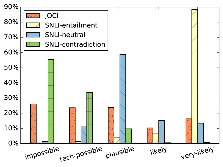
(a) JOCI vs. SNLI

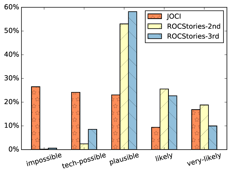
(b) JOCI vs. ROCStories

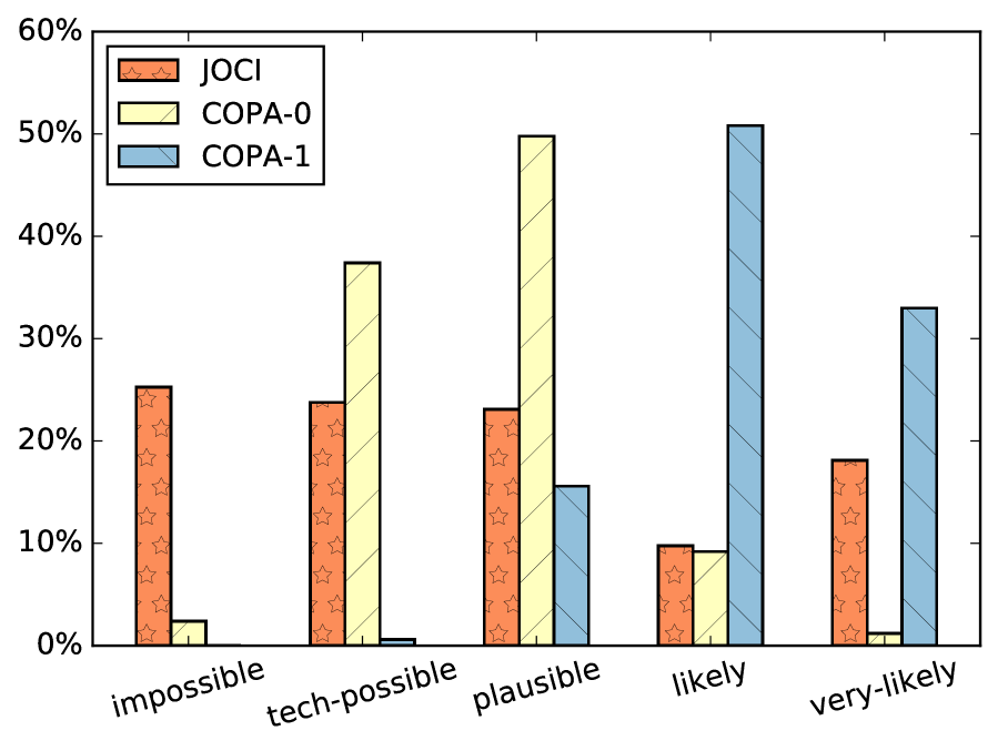
(c) JOCI vs. COPA

Figure 6: Comparison of normalized distributions between JOCI and other corpora.

Quality: We measure the quality of each pair by calculating Cohen’s $\kappa$ of workers’ annotations. The average $\kappa$ of the JOCI corpus is 0.54. Fig 7 shows the growth of the size of JOCI as we decrease the threshold of the averaged $\kappa$ to filter pairs. Even if we place a relatively strict threshold ($>$0.6), we still get a large subset of JOCI with over 20K pairs. Table 2 contains pairs randomly sampled from this subset, qualitatively confirming we can generate and collect annotations of pairs at each ordinal category.

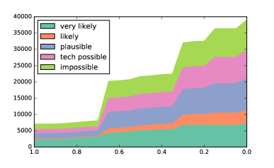
Figure 7: Data growth along averaged $\kappa$ scores.

Label Distribution: We believe datasets with wide support of label distribution are important in training and evaluating systems to recognize ordinal scale inferences. Fig 6(a) shows the normalized label distribution of JOCI vs. SNLI. As desired, JOCI covers a wide range of ordinal likelihoods, with many samples in each ordinal scale. Note also how traditional RTE labels are related to ordinal labels, although many inferences in SNLI require no common-sense knowledge (e.g. paraphrases). As expected, entailments are mostly considered very likely; neutral inferences mostly plausible; and contradictions likely to be either impossible or technically possible.

Fig 6(b) shows the normalized distributions of JOCI and ROCStories. Compared with ROCStories, JOCI still covers a wider range of ordinal likelihood. We observe in ROCStories that, while 2nd sentences are in general more likely to be true than 3rd, a large proportion of both 2nd and 3rd sentences are plausible, as compared to likely or very likely. This matches intuition: pragmatics dictates that subsequent sentences in a standard narrative carry new information. That our protocol picks this up is an encouraging sign for our ordinal protocol, as well as suggestive that the makeup of the elicited ROCStories collection is indeed “story like.”

For the COPA dataset, we make use only of the pairs in which the alternatives are plausible effects (rather than causes) of the premise, as our protocol more easily accommodates these pairs. Annotating this section of COPA with ordinal labels provides an enlightening and validating view of the dataset. Fig 6(c) shows the normalized distribution of COPA next to that of JOCI. (COPA-1 alternatives are marked as most plausible; COPA-0 are not.) True to its name, the majority of COPA alternatives are labeled as either plausible or likely; almost none are impossible. This is consistent with the idea that the COPA task is to determine which of two possible options is the more plausible. Fig 8 shows the joint distribution of ordinal labels on (COPA-0,COPA-1) pairs. As expected, the densest areas of the heatmap lie above the diagonal, indicating that in almost every pair, COPA-1 received a higher likelihood judgement than COPA-0.

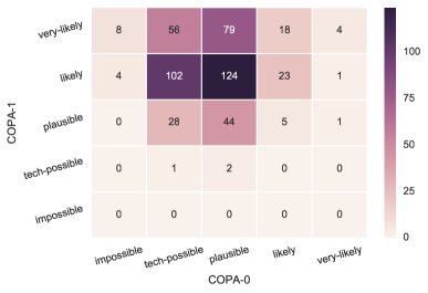
Figure 8: COPA heatmap.

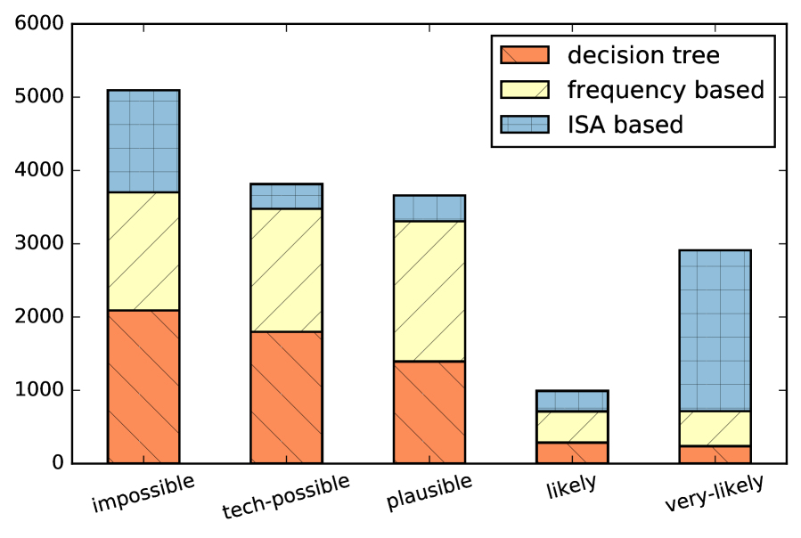
(a) Distribution of AGCI-wk

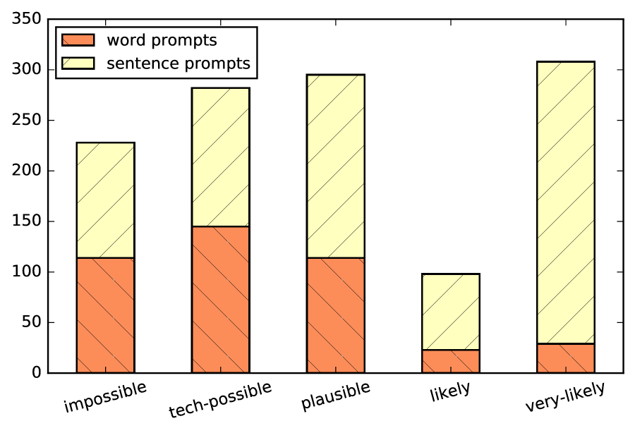
(b) Distribution of AGCI-nn

Figure 9: Label distributions of AGCI.

Automatic Generation Comparisons: We compare the label distributions of different methods for automatic generation of common-sense inference (AGCI) in Fig 9. Among ACGI-wk (generation based on world knowledge) methods, the ISA strategy yields a bimodal distribtuion, with the majority of inferences labeled impossible or very likely. This is likely because most copular statements generated with the ISA strategy will either be categorically true or false. In contrast, the decision tree and frequency based strategies generate many more hypotheses with intermediate ordinal labels. This suggests the propositional templates (learned from text) capture many “possibilistic” hypotheses, which is our aim.

The two AGCI-nn (generation via neural methods) strategies show interesting differences in label distribution as well. Sequence-to-sequence decodings with full-sentence prompts lead to more very likely labels than single-word prompts. The reason may be that the model behaves more similarly to SNLI entailments when it has access to all the information in the context. When combined, the five AGCI strategies (three AGCI-wk and two AGCI-nn) provide reasonable coverage over all five categories, as can be seen in Fig 6.

6 Predicting Ordinal Judgments

We want to be able to predict ordinal judgments of the kind presented in this corpus. Our goal in this section is to establish baseline results and explore what kinds of features are useful for predicting ordinal common-sense inference. To do so, we train and test a logistic ordinal regression model $g_{\theta}(\phi({\mathcal{C}},{\mathcal{H}}))$, which outputs ordinal labels using features $\phi$ defined on context-inference pairs. Here, $g_{\theta}(\cdot)$ is a regression model with $\theta$ as trained parameters; we train using the margin-based method of [Rennie and Srebro (2005], implemented in [Pedregosa-Izquierdo (2015], with the following features:

Bag of words features (bow): We compute (1) “BOW overlap” (size of word overlap in $\mathcal{C}$ and $\mathcal{H}$), and (2) BOW overlap divided by the length of $\mathcal{H}$.

Similarity features (sim): Using Google’s word2vec vectors trained on 100 billion tokens of GoogleNews, we (1) sum the vectors in both the context and hypothesis and compute the cosine-similarity of the resulting two vectors (“similarity of average”), and (2) compute the cosine-similarity of all word pairs across the context and inference, then average those similarities (“average of similarity”).

Seq2seq score features (s2s): We compute the log probability $\log P(\mathcal{H}|\mathcal{C})$ under the sequence-to-sequence model described in § 4.1.2. There are five variants: (1) Seq2seq trained on SNLI “entailment” pairs only, (2) “neutral” pairs only, (3) “contradiction” pairs only, (4) “neutral” and “contradiction” pairs, and (5) SNLI pairs (any label) with the context (premise) replaced by an empty string.

Seq2seq binary features (s2s-bin): Binary indicator features for each of the five seq2seq model variants, indicating that model achieved the lowest score on the context-hypothesis pair.

Length features (len): This set comprises three features: the length of the context (in tokens), the difference in length between the context and hypothesis, and a binary feature indicating if the hypothesis is longer than the context.

6.1 Analysis

We train and test our regression model on two subsets of the JOCI corpus, which, for brevity, we call “A” and “B.” “A” consists of 2,976 sentence pairs (i.e., context-hypothesis pairs) from SNLI-train annotated with ordinal labels. This corresponds to the three rows labeled SNLI in Table 1 ($993+988+995=2,976$ pairs), and can be viewed as a textual entailment dataset re-labeled with ordinal judgments. “B” consists of 6,375 context-inference pairs, in which the contexts are the same 2,976 SNLI-train premises as “A”, and the hypotheses are generated based on world knowledge (§4.1.1); these pairs are also annotated with ordinal labels. This corresponds to a subset of the row labeled AGCI in Table 1. A key difference between “A” and “B” is that the hypotheses in “A” are human-elicited, while those in “B” are auto-generated; we are interested in seeing whether this affects the task’s difficulty.

Model	A-train	A-test	B-train	B-test
Regression: $g_{\theta}(\cdot)$	2.05	1.96	2.48	2.74
Most Frequent	5.70	5.56	6.55	7.00
Freq. Sampling	4.62	4.29	5.61	5.54
Rounded Average	2.46	2.39	2.79	2.89
One-vs-All	3.74	3.80	5.14	5.71

Table 4: Mean squared error.

Model	A-train	A-test	B-train	B-test
Regression: $g_{\theta}(\cdot)$	.39*	.40*	.32*	.27*
Most Frequent	.00*	.00*	.00*	.00*
Freq. Sampling	.03*	.10*	.01*	.01*
Rounded Average	.00*	.00*	.00*	.00*
One-vs-All	.31*	.30*	.28*	.24*

Table 5: Spearman’s $\rho$. (*p-value$<$.01)

Tables 4 and 5 show each model’s performance (mean squared error and Spearman’s $\rho$, respectively) in predicting ordinal labels. We compare our ordinal regression model $g_{\theta}(\cdot)$ with these baselines:

Most Frequent: Select the ordinal class appearing most often in train.

Frequency Sampling: Select an ordinal label according to their distribution in train.

Rounded Average: Average over all labels from train rounded to nearest ordinal.

One-vs-All: Train one SVM classifier per ordinal class and select the class label with the largest corresponding margin. We train this model with the same set of features as the ordinal regression model.

Overall, the regression model achieves the lowest MSE and highest $\rho$, implying that this dataset is learnable and tractable. Naturally, we would desire a model that achieves MSE under 1.0, and we hope that the release of our dataset will encourage more concerted effort in this common-sense inference task. Importantly, note that performance on A-test is better than on B-test. We believe “B” is a more challenging dataset because auto-generation of hypothesis leads to wider variety than elicitation.

	MSE		Spear. $\rho$
Feature Set	A	B	A	B
all	1.96	2.74	.40*	.27*
all – {sim}	2.10	2.75	.34*	.25*
all – {bow}	2.02	2.77	.37*	.25*
all – {sim,bow}	2.31	2.79	.16*	.20*
all – {s2s}	2.00	2.85	.38*	.22*
all – {s2s-bin}	1.97	2.76	.40*	.26*
all – {s2s,s2s-bin}	2.06	2.87	.35*	.21*
all – {len}	2.01	2.77	.39*	.25*
$\varnothing$ + {sim}	2.06	3.04	.35*	.10*
$\varnothing$ + {bow}	2.10	2.89	.34*	.12*
$\varnothing$ + {s2s}	2.33	2.80	.14*	.20*
$\varnothing$ + {s2s-bin}	2.39	2.89	.00*	.00*
$\varnothing$ + {len}	2.39	2.89	.00*	.05*

Table 6: Ablation results for ordinal regression model on A-test and B-test. (*p-value$<$.01 for $\rho$)

We also run a feature ablation test. Table 6 shows that the most useful features differ for A-test and B-test. On A-test, where the inferences are elicited from humans, removal of similarity- and bow-based features together results in the largest performance drop. On B-test, by contrast, removing similarity and bow features results in a comparable performance drop to removing seq2seq features. These observations point to statistical differences between human-elicited and auto-generated hypotheses, a motivating point of the JOCI corpus.

7 Conclusions and Future Work

In motivating the need for automatically building collections of common-sense knowledge, ?) wrote:

“China launched a meteorological satellite into orbit Wednesday.” suggests to a human reader that (among other things) there was a rocket launch; China probably owns the satellite; the satellite is for monitoring weather; the orbit is around Earth; etc

The use of “etc” summarizes an infinite number of other statements that a human reader would find to be very likely, likely, technically plausible, or impossible, given the provided context.

Preferably we could build systems that would automatically learn common-sense exclusively from available corpora; extracting not just statements about what is possible, but also the associated probabilities of how likely certain things are to obtain in any given context. We are unaware of existing work that has demonstrated this to be feasible.

We have thus described a multi-stage approach to common-sense textual inference: we first extract large numbers of possible statements from a corpus, and use those statements to generate contextually grounded context-hypothesis pairs. These are presented to humans for direct assessment of subjective likelihood, rather than relying on corpus data alone. As the data is automatically generated, we seek to bypass issues in human elicitation bias. Further, since subjective likelihood judgments are not difficult for humans, our crowdsourcing technique is both inexpensive and scalable.

Future work will extend our techniques for forward inference generation, further scale up the annotation of additional examples, and explore the use of larger, more complex contexts. The resulting JOCI corpus will be used to improve algorithms for natural language inference tasks such as storytelling and story understanding.

References

- [Agirre et al. (2012] Eneko Agirre, Mona Diab, Daniel Cer, and Aitor Gonzalez-Agirre. 2012. Semeval-2012 task 6: A pilot on semantic textual similarity. In Proceedings of the Sixth International Workshop on Semantic Evaluation.
- [Agresti (2003] A. Agresti. 2003. Categorical Data Analysis. Wiley Series in Probability and Statistics. Wiley.
- [Baccianella et al. (2009] Stefano Baccianella, Andrea Esuli, and Fabrizio Sebastiani. 2009. Evaluation measures for ordinal regression. In 2009 Ninth international conference on intelligent systems design and applications, pages 283–287. IEEE.
- [Bahdanau et al. (2014] Dzmitry Bahdanau, Kyunghyun Cho, and Yoshua Bengio. 2014. Neural machine translation by jointly learning to align and translate. CoRR, abs/1409.0473.
- [Baker et al. (1998] Collin F. Baker, Charles J. Fillmore, and John B. Lowe. 1998. The berkeley framenet project. In Proceedings of the 36th Annual Meeting of the Association for Computational Linguistics and 17th International Conference on Computational Linguistics, Volume 1, pages 86–90, Montreal, Quebec, Canada, August. Association for Computational Linguistics.
- [Banko and Etzioni (2007] Michele Banko and Oren Etzioni. 2007. Strategies for Lifelong Knowledge Extraction from the Web. In Proceedings of K-CAP.
- [Beltagy et al. (2016] I Beltagy, Stephen Roller, Pengxiang Cheng, Katrin Erk, and Raymond J Mooney. 2016. Representing meaning with a combination of logical and distributional models. Computational Linguistics.
- [Bennett and Lanning (2007] James Bennett and Stan Lanning. 2007. The netflix prize. In Proceedings of KDD cup and workshop, volume 2007, page 35.
- [Berant et al. (2011] Jonathan Berant, Ido Dagan, and Jacob Goldberger. 2011. Global learning of typed entailment rules. In Proceedings of ACL.
- [Bowman et al. (2015] Samuel R. Bowman, Gabor Angeli, Christopher Potts, and Christopher D. Manning. 2015. A large annotated corpus for learning natural language inference. In Proceedings of the 2015 Conference on Empirical Methods in Natural Language Processing (EMNLP). Association for Computational Linguistics.
- [Chambers and Jurafsky (2008] Nathanael Chambers and Dan Jurafsky. 2008. Unsupervised Learning of Narrative Event Chains. In Proceedings of ACL.
- [Chklovski (2003] Timothy Chklovski. 2003. LEARNER: A System for Acquiring Commonsense Knowledge by Analogy. In Proceedings of Second International Conference on Knowledge Capture (K-CAP 2003).
- [Clark and Weir (1999] Stephen Clark and David Weir. 1999. An iterative approach to estimating frequencies over a semantic hierarchy. In Proceedings of EMNLP.
- [Clark et al. (2003] Peter Clark, Phil Harrison, and John Thompson. 2003. A knowledge-driven approach to text meaning processing. In Proceedings of the HLT-NAACL 2003 workshop on Text meaning-Volume 9, pages 1–6. Association for Computational Linguistics.
- [Clark (1975] Herbert H. Clark. 1975. Bridging. In R. C. Schank and B. L. Nash-Webber, editors, Theoretical issues in natural language processing. Association for Computing Machinery, New York.
- [Cooper et al. (1996] Robin Cooper, Dick Crouch, Jan Van Eijck, Chris Fox, Johan Van Genabith, Jan Jaspars, Hans Kamp, David Milward, Manfred Pinkal, Massimo Poesio, et al. 1996. Using the framework. Technical report, Technical Report LRE 62-051 D-16, The FraCaS Consortium.
- [Dagan et al. (2006] Ido Dagan, Oren Glickman, and Bernardo Magnini. 2006. The pascal recognising textual entailment challenge. In Machine learning challenges. evaluating predictive uncertainty, visual object classification, and recognising tectual entailment.
- [de Haan (1997] F. de Haan. 1997. The Interaction of Modality and Negation: A Typological Study. A Garland Series. Garland Pub.
- [de Marneffe et al. (2014] Marie-Catherine de Marneffe, Timothy Dozat, Natalia Silveira, Katri Haverinen, Filip Ginter, Joakim Nivre, and Christopher D Manning. 2014. Universal stanford dependencies: A cross-linguistic typology. In LREC, volume 14, pages 4585–4592.
- [Erk et al. (2010] Katrin Erk, Sebastian Padó, and Ulrike Padó. 2010. A flexible, corpus-driven model of regular and inverse selectional preferences. Computational Linguistics, 36(4):723–763.
- [Ferraro et al. (2014] Francis Ferraro, Max Thomas, Matthew R. Gormley, Travis Wolfe, Craig Harman, and Benjamin Van Durme. 2014. Concretely Annotated Corpora. In 4th Workshop on Automated Knowledge Base Construction (AKBC).
- [Friedland et al. (2004] Noah S Friedland, Paul G Allen, Gavin Matthews, Michael Witbrock, David Baxter, Jon Curtis, Blake Shepard, Pierluigi Miraglia, Jurgen Angele, Steffen Staab, et al. 2004. Project halo: Towards a digital aristotle. AI magazine, 25(4):29.
- [Garrette et al. (2011] Dan Garrette, Katrin Erk, and Raymond Mooney. 2011. Integrating logical representations with probabilistic information using markov logic. In Proceedings of the Ninth International Conference on Computational Semantics, pages 105–114. Association for Computational Linguistics.
- [Gaudette and Japkowicz (2009] Lisa Gaudette and Nathalie Japkowicz. 2009. Evaluation methods for ordinal classification. In Proceedings of the 22Nd Canadian Conference on Artificial Intelligence: Advances in Artificial Intelligence, Canadian AI ’09, pages 207–210, Berlin, Heidelberg. Springer-Verlag.
- [Gella et al. (2013] Spandana Gella, Paul Cook, and Bo Han. 2013. Unsupervised word usage similarity in social media texts. Atlanta, Georgia, USA, page 248.
- [Giampiccolo et al. (2008] Danilo Giampiccolo, Hoa Trang Dang, Bernardo Magnini, Ido Dagan, Elena Cabrio, and Bill Dolan. 2008. The fourth pascal recognizing textual entailment challenge. In Proceedings of TAC 2008.
- [Gordon and Van Durme (2013] Jonathan Gordon and Benjamin Van Durme. 2013. Reporting bias and knowledge extraction. In Automated Knowledge Base Construction (AKBC): The 3rd Workshop on Knowledge Extraction at CIKM.
- [Havasi et al. (2007] Catherine Havasi, Robert Speer, and Jason Alonso. 2007. ConceptNet 3: a Flexible, Multilingual Semantic Network for Common Sense Knowledge. In Proceedings of RANLP.
- [Hearst (1992] Marti Hearst. 1992. Automatic Acquisition of Hyponyms from Large Text Corpora. In Proceedings of COLING.
- [Hobbs and Navarretta (1993] Jerry R. Hobbs and Costanza Navarretta. 1993. Methodology for knowledge acquisition (unpublished manuscript). http://www.isi.edu/h̃obbs/damage.text.
- [Hobbs (1987] Jerry R. Hobbs. 1987. World Knowledge And Word Meaning. Theoretical Issues In Natural Language Processing.
- [Hochreiter and Schmidhuber (1997] Sepp Hochreiter and Jürgen Schmidhuber. 1997. Long short-term memory. Neural computation, 9(8):1735–1780.
- [Horn (1989] L.R. Horn. 1989. A Natural History of Negation. David Hume series. CSLI.
- [Lenat (1995] Douglas B Lenat. 1995. Cyc: A large-scale investment in knowledge infrastructure. Communications of the ACM, 38(11):33–38.
- [Levesque et al. (2011] Hector J. Levesque, Ernest Davis, and Leora Morgenstern. 2011. The winograd schema challenge. In AAAI Spring Symposium: Logical Formalizations of Commonsense Reasoning.
- [Liakata and Pulman (2002] Maria Liakata and Stephen Pulman. 2002. From Trees to Predicate Argument Structures. In Proceedings of COLING.
- [Lin and Pantel (2001] Dekang Lin and Patrick Pantel. 2001. DIRT - Discovery of Inference Rules from Text. In Proceedings of KDD.
- [Liu et al. (2015] Quan Liu, Hui Jiang, Si Wei, Zhen-Hua Ling, and Yu Hu. 2015. Learning semantic word embeddings based on ordinal knowledge constraints. In Proceedings of the 53rd Annual Meeting of the Association for Computational Linguistics and the 7th International Joint Conference on Natural Language Processing (ACL-IJCNLP), pages 1501–1511.
- [Lyons (1977] J. Lyons. 1977. Semantics. Semantics. Cambridge University Press.
- [MacCartney and Manning (2007] Bill MacCartney and Christopher D. Manning. 2007. Natural logic for textual inference. In Proceedings of ACL: Workshop on Textual Entailment and Paraphrasing.
- [Marelli et al. (2014] Marco Marelli, Stefano Menini, Marco Baroni, Luisa Bentivogli, Raffaella Bernardi, and Roberto Zamparelli. 2014. A SICK cure for the evaluation of compositional distributional semantic models. In Proceedings of the Ninth International Conference on Language Resources and Evaluation (LREC-2014), Reykjavik, Iceland, May 26-31, 2014., pages 216–223.
- [McCarthy (1959] John McCarthy. 1959. Programs with common sense. In Proceedings of the Teddington Conference on the Mechanization of Thought Processes, London: Her Majesty’s Stationery Office.
- [McRae et al. (1998] Ken McRae, Michael J. Spivey-Knowlton, and Michael K. Tanenhaus. 1998. Modeling the influence of thematic fit (and other constraints) in on-line sentence comprehension. JOURNAL OF MEMORY AND LANGUAGE, 38:283–312.
- [McRae et al. (2005] Ken McRae, George S. Cree, Mark S. Seidenberg, and Chris McNorgan. 2005. Semantic feature production norms for a large set of living and nonliving things. Behavior Research Methods, Instruments, & Computers, 37(4):547–559.
- [Miller (1995] George A Miller. 1995. Wordnet: a lexical database for english. Communications of the ACM, 38(11):39–41.
- [Misra et al. (2016] Ishan Misra, C. Lawrence Zitnick, Margaret Mitchell, and Ross Girshick. 2016. Seeing through the human reporting bias: Visual classifiers from noisy human-centric labels. In Proceedings of CVPR.
- [Mostafazadeh et al. (2016] Nasrin Mostafazadeh, Nathanael Chambers, Xiaodong He, Devi Parikh, Dhruv Batra, Lucy Vanderwende, Pushmeet Kohli, and James Allen. 2016. A corpus and cloze evaluation for deeper understanding of commonsense stories. In Proceedings of the 2016 Conference of the North American Chapter of the Association for Computational Linguistics: Human Language Technologies, pages 839–849, San Diego, California, June. Association for Computational Linguistics.
- [Paşca and Van Durme (2007] Marius Paşca and Benjamin Van Durme. 2007. What You Seek is What You Get: Extraction of Class Attributes from Query Logs. In Proceedings of IJCAI.
- [Padó et al. (2009] Ulrike Padó, Matthew W. Crocker, Frank Keller, and Matthew W. Crocker. 2009. A probabilistic model of semantic plausibility in sentence processing. Cognitive Science, 33(5):795–838.
- [Pantel et al. (2007] Patrick Pantel, Rahul Bhagat, Bonaventura Coppola, Timothy Chklovski, and Eduard H Hovy. 2007. Isp: Learning inferential selectional preferences. In HLT-NAACL, pages 564–571.
- [Paperno et al. (2016] Denis Paperno, Germán Kruszewski, Angeliki Lazaridou, Ngoc Quan Pham, Raffaella Bernardi, Sandro Pezzelle, Marco Baroni, Gemma Boleda, and Raquel Fernandez. 2016. The lambada dataset: Word prediction requiring a broad discourse context. In Proceedings of the 54th Annual Meeting of the Association for Computational Linguistics (Volume 1: Long Papers), pages 1525–1534, Berlin, Germany, August. Association for Computational Linguistics.
- [Parker et al. (2011] Robert Parker, David Graff, Junbo Kong, Ke Chen, and Kazuaki Maeda. 2011. English gigaword fifth edition, june. Linguistic Data Consortium, LDC2011T07.
- [Pasca (2008] Marius Pasca. 2008. Turning web text and search queries into factual knowledge: Hierarchical class attribute extraction.
- [Pedregosa-Izquierdo (2015] Fabian Pedregosa-Izquierdo. 2015. Feature extraction and supervised learning on fMRI: from practice to theory. Ph.D. thesis, Université Pierre et Marie Curie-Paris VI.
- [Pichotta and Mooney (2016] Karl Pichotta and Raymond J Mooney. 2016. Learning statistical scripts with lstm recurrent neural networks. In Proceedings of the 30th AAAI Conference on Artificial Intelligence (AAAI).
- [Popescu and Dinu (2009] Marius Popescu and Liviu P Dinu. 2009. Comparing statistical similarity measures for stylistic multivariate analysis. In RANLP, pages 349–354.
- [Rennie and Srebro (2005] Jason DM Rennie and Nathan Srebro. 2005. Loss functions for preference levels: Regression with discrete ordered labels. In Proceedings of the IJCAI multidisciplinary workshop on advances in preference handling, pages 180–186. Kluwer Norwell, MA.
- [Resnik (1993] Philip Resnik. 1993. Semantic classes and syntactic ambiguity. In Proceedings of ARPA Workshop on Human Language Technology.
- [Richardson and Domingos (2006] Matthew Richardson and Pedro Domingos. 2006. Markov logic networks. Machine learning, 62(1-2):107–136.
- [Richardson et al. (1998] Stephen D. Richardson, William B. Dolan, and Lucy Vanderwende. 1998. MindNet: Acquiring and Structuring Semantic Information from Text. In Proceedings of ACL.
- [Roemmele et al. (2011] Melissa Roemmele, Cosmin Adrian Bejan, and Andrew S. Gordon. 2011. Choice of Plausible Alternatives: An Evaluation of Commonsense Causal Reasoning. In AAAI Spring Symposium on Logical Formalizations of Commonsense Reasoning, Stanford University, March.
- [Rudinger et al. (2015] Rachel Rudinger, Pushpendre Rastogi, Francis Ferraro, and Benjamin Van Durme. 2015. Script induction as language modeling. In Proceedings of EMNLP.
- [Saurí and Pustejovsky (2009] Roser Saurí and James Pustejovsky. 2009. Factbank: A corpus annotated with event factuality. Language resources and evaluation, 43(3):227–268.
- [Sayeed et al. (2015] Asad Sayeed, Vera Demberg, and Pavel Shkadzko. 2015. An exploration of semantic features in an unsupervised thematic fit evaluation framework. Italian Journal of Computational Linguistics, 1(1).
- [Schank (1975] Roger C. Schank. 1975. Using knowledge to understand. In TINLAP ’75: Proceedings of the 1975 workshop on Theoretical issues in natural language processing.
- [Schubert (2002] Lenhart Schubert. 2002. Can we derive general world knowledge from texts? In Proceedings of the second international conference on Human Language Technology Research, pages 94–97. Morgan Kaufmann Publishers Inc.
- [Singh (2002] Push Singh. 2002. The public acquisition of commonsense knowledge. In Proceedings of AAAI Spring Symposium: Acquiring (and Using) Linguistic (and World) Knowledge for Information Access. AAAI.
- [Snow et al. (2006] Rion Snow, Daniel Jurafsky, and Andrew Y. Ng. 2006. Semantic Taxonomy Induction from Heterogenous Evidence. In Proceedings of COLING-ACL.
- [Suchanek et al. (2007] Fabian M. Suchanek, Gjergji Kasneci, and Gerhard Weikum. 2007. YAGO: A Core of Semantic Knowledge Unifying WordNet and Wikipedia. In Proceedings of WWW.
- [Tanenhaus and Seidenberg (1980] Michael K. Tanenhaus and Mark S. Seidenberg. 1980. Discourse context and sentence perception. Technical Report 176, Center for the Study of Reading, Illinois University, Urbana.
- [Thomason (1972] Richmond H. Thomason. 1972. A Semantic Theory of Sortal Incorrectness. Journal of Philosophical Logic, 1(2):209–258, May.
- [Van Durme and Schubert (2008] Benjamin Van Durme and Lenhart Schubert. 2008. Open knowledge extraction through compositional language processing. In Proceedings of the 2008 Conference on Semantics in Text Processing, pages 239–254. Association for Computational Linguistics.
- [Van Durme et al. (2009] Benjamin Van Durme, Phillip Michalak, and Lenhart Schubert. 2009. Deriving generalized knowledge from corpora using WordNet abstraction. In Proceedings of the 12th Conference of the European Chapter of the ACL (EACL 2009), pages 808–816, Athens, Greece, March. Association for Computational Linguistics.
- [Van Durme (2010] Benjamin Van Durme. 2010. Extracting implicit knowledge from text. Ph.D. thesis, University of Rochester, Department of Computer Science, Rochester, NY 14627-0226.
- [Vinyals et al. (2015] Oriol Vinyals, Ł ukasz Kaiser, Terry Koo, Slav Petrov, Ilya Sutskever, and Geoffrey Hinton. 2015. Grammar as a foreign language. In C. Cortes, N. D. Lawrence, D. D. Lee, M. Sugiyama, and R. Garnett, editors, Advances in Neural Information Processing Systems 28, pages 2773–2781. Curran Associates, Inc.
- [White et al. (2016] Aaron Steven White, Drew Reisinger, Keisuke Sakaguchi, Tim Vieira, Sheng Zhang, Rachel Rudinger, Kyle Rawlins, and Benjamin Van Durme. 2016. Universal decompositional semantics on universal dependencies. In EMNLP.
- [Young et al. (2014] Peter Young, Alice Lai, Micah Hodosh, and Julia Hockenmaier. 2014. From image descriptions to visual denotations: New similarity metrics for semantic inference over event descriptions. Transactions of the Association for Computational Linguistics, 2:67–78.
- [Zernik (1992] Uri Zernik. 1992. Closed yesterday and closed minds: Asking the right questions of the corpus to distinguish thematic from sentential relations. In Proceedings of COLING.