Quiver relations and associated symmetric polynomials

Abstract

The idea is to identify certain path algebra elements with symmetric functions. We propose such a morphism by solving the quiver relations, which describe the Plucker-type embedding for quiver grassmannians.

1 Introduction

Quiver is a directed graph with multiply edges and loops allowed. Let $Q$ = finite quiver with $k$ vertices and $l$ arrows. Quiver representation $M$ is a collection of vector spaces and linear maps, attached to each vertex and arrow of $Q$:

$$M=\{V_{1},\dots,V_{k}\}\cup\{M_{v,i,j}\},\quad\mathrm{dim}(V_{i})=d_{i},\quad M_{v,i,j}=Mat(d_{i}\times d_{j},\mathrm{k}):V_{i}\rightarrow V_{j}$$ (1)

Quiver grassmannian $Gr_{\underline{e}}(Q,M)$ of dimension vector $\underline{e}=(e_{1},\dots,e_{k})$ contains all $\underline{e}$-dimensional subspaces of $M$, compatible with the underlying linear maps.

Fix an ordered basis $\mathcal{B}=\{1,2,\dots,d_{1},d_{1}+1,\dots,d_{l}\}$, $I\subset B$ for all $V_{i}$s. Quiver relations (QR) are of the form [4]:

$$\sum_{s^{\prime},t^{\prime}}(-1)^{\epsilon(s^{\prime},t^{\prime})}M_{v,s^{\prime},t^{\prime}}\ \Delta_{s}^{s^{\prime}}\ \Delta_{t^{\prime}}^{t}-\ \sum_{s^{\prime}}(-1)^{\epsilon(s^{\prime},t)}M_{v,s^{\prime},t}\ \Delta_{s}^{s^{\prime}}\ \Delta_{I}=0,\quad I\subset\mathcal{B},\quad|I|=e$$ (2)

Define $Fset$ as a collection of all non-vanishing $\Delta^{i}_{j}$’s in 2. Our aim is to generate polynomials which are sums of $GL$ characters with coefficients given by the embedding

$$Gr_{\overline{(}e)}(Q,M)\xrightarrow{\phi_{1}}Gr(e,d)\xrightarrow{\phi_{2}}\mathbb{P}^{e+d-1},\quad e=\sum e_{i},d=\sum d_{i}$$ (3)

Define 2 kind of invariants:

$$P(Q,s,\mathbf{M})=\sum\limits_{R}\Delta_{R}\chi_{R}(\overline{t})$$ (4)

with $\Delta=$ homogeneous coordinate on the image of embedding 3, and

$$\tilde{P}(Q,s,\mathbf{M})=\sum\limits_{R^{\prime}}\tilde{\Delta}_{R^{\prime}}\chi_{R}(\overline{t})$$ (5)

with $\tilde{\Delta}\in Fset$ only (PR are not taken into part). Note that $P,P^{\prime}$ are inhomogeneous in $R,R^{\prime}$ (may contain Young diagrams of different size).
Proposition 1. In case of $\chi_{\lambda}=s_{\lambda}$ polynomials $P(Q,s,\mathbf{M})$ form a basis of Symm algebra. This seems to be obvious, but not the only one possible choice of $\chi$.
Write $\mathbf{M}$ as block matrix:

$$\mathbf{M}=\left[\begin{array}[]{cccc}M_{{1,1}}&M_{{1,2}}&M_{{1,3}}&\dots\\ \vskip 6.0pt plus 2.0pt minus 2.0pt\cr M_{{2,1}}&M_{{2,2}}&M_{{2,3}}&\\ \vskip 6.0pt plus 2.0pt minus 2.0pt\cr M_{{3,1}}&M_{{3,2}}&M_{{3,3}}&\\ \vskip 6.0pt plus 2.0pt minus 2.0pt\cr\vdots&&&\ddots\end{array}\right]$$ (6)

with each $M_{i,j}$ corresponding to $(i,j)$ linear map.

2 Computation of $P,\tilde{P}$. Quiver relations as vanishing minors

2.1 $Q=A_{2}$, $M=\{\mathbb{C},\mathbb{C},\mu=Mat(2,2,\mathbb{C})\},\overline{e}=(1,1)$

$I=\{2,4\}$: One non-trivial equation, $\#(+,-)=(2,2)$

$$F\left(v,2,3\right)=\mu_{{v,1,4}}\Delta_{{\left\{1,4\right\}}}\Delta_{{\left\{2,3\right\}}}+\mu_{{v,2,4}}\Delta_{{\left\{2,4\right\}}}\Delta_{{\left\{2,3\right\}}}-\mu_{{v,1,3}}\Delta_{{\left\{1,4\right\}}}\Delta_{{\left\{2,4\right\}}}-\mu_{{v,2,3}}{\Delta_{{\left\{2,4\right\}}}}^{2}=0$$ (7)

Or:

$$F\left(v,2,3\right)=\left|\begin{array}[]{ccc}\mu_{{v,1,4}}&0&\Delta_{{\left\{2,4\right\}}}\\ \vskip 6.0pt plus 2.0pt minus 2.0pt\cr\mu_{{v,2,4}}&\Delta_{{\left\{1,4\right\}}}&{\frac{\mu_{{v,2,3}}{\Delta_{{\left\{2,4\right\}}}}^{2}}{\mu_{{v,1,4}}\Delta_{{\left\{2,3\right\}}}}}\\ \vskip 6.0pt plus 2.0pt minus 2.0pt\cr\mu_{{v,1,3}}&\Delta_{{\left\{2,3\right\}}}&\Delta_{{\left\{2,3\right\}}}\end{array}\right|=\left|\begin{array}[]{ccc}\mu_{{v,1,4}}&\Delta_{{\left\{2,4\right\}}}&\Delta_{{\left\{2,4\right\}}}\\ \vskip 6.0pt plus 2.0pt minus 2.0pt\cr-\mu_{{v,2,4}}&\Delta_{{\left\{1,4\right\}}}&-{\frac{\mu_{{v,2,3}}\Delta_{{\left\{2,4\right\}}}}{\mu_{{v,1,3}}}}\\ \vskip 6.0pt plus 2.0pt minus 2.0pt\cr\mu_{{v,1,3}}&0&\Delta_{{\left\{2,3\right\}}}\end{array}\right|=0$$ (8)

$$,\quad\Delta_{1,2}=0,\quad\Delta_{3,4}=0$$ (9)

Note that if we inverse the arrow, our equation will change:

$$F\left(v,4,1\right)=\mu^{\prime}_{{v,3,2}}\Delta_{{\left\{2,3\right\}}}\Delta_{{\left\{1,4\right\}}}+\mu^{\prime}_{{v,4,2}}\Delta_{{\left\{2,4\right\}}}\Delta_{{\left\{1,4\right\}}}-\mu^{\prime}_{{v,3,1}}\Delta_{{\left\{2,3\right\}}}\Delta_{{\left\{2,4\right\}}}-\mu^{\prime}_{{v,4,1}}{\Delta_{{\left\{2,4\right\}}}}^{2}=0,$$ (10)

where $\mu^{\prime}$ is the inverse map. Now fix $\mu=\left(\begin{array}[]{cc}p&1-p\\ \vskip 6.0pt plus 2.0pt minus 2.0pt\cr 1-p&p\end{array}\right)$ – quantum permutation matrix from https://arxiv.org/abs/1109.4888. Combining this with the only Plu"cker identity

$$\Delta_{{\left\{1,2\right\}}}\Delta_{{\left\{3,4\right\}}}-\Delta_{{\left\{1,3\right\}}}\Delta_{{\left\{2,4\right\}}}+\Delta_{{\left\{1,4\right\}}}\Delta_{{\left\{2,3\right\}}}=0$$ (11)

we obtain our polynomial invariant:

$$\boxed{P(A_{2},4,\mu)=Qh_{{1}}-{\frac{Q\left(-Wp-Q+pQ\right)h_{{2}}}{W-Wp+pQ}}+W\left({h_{{1}}}^{2}-h_{{2}}h_{{0}}\right)-{\frac{\left(-Wp-Q+pQ\right)W\left(h_{{1}}h_{{2}}-h_{{3}}h_{{0}}\right)}{W-Wp+pQ}}}$$ (12)

where $Q,W$ are arbitrary complex numbers.

2.2 $M=\{\mathbb{C}^{2},\mathbb{C}^{2},\mu=Mat(4,4,\mathbb{C})\},\overline{e}=(2,2)$

$I={3,4,7,8}$: We have 2x2 non-trivial quiver equations () with $\#(+,-)=(4,5),(6,3)$ One of them ()

$$F(v,3,5)=\left|\begin{array}[]{ccc}\mu_{{v,1,7}}+\mu_{{v,2,7}}+\mu_{{v,2,8}}&\Delta_{{\left\{3,4,7,8\right\}}}&\Delta_{{\left\{3,4,5,7\right\}}}+2\,\Delta_{{\left\{3,4,7,8\right\}}}\\ \vskip 6.0pt plus 2.0pt minus 2.0pt\cr\mu_{{v,3,8}}-\mu_{{v,3,7}}-\mu_{{v,1,5}}&\Delta_{{\left\{1,4,7,8\right\}}}+2\,\Delta_{{\left\{2,4,7,8\right\}}}&0\\ \vskip 6.0pt plus 2.0pt minus 2.0pt\cr-\mu_{{v,1,8}}+\mu_{{v,2,5}}+{\frac{\mu_{{v,3,5}}\Delta_{{\left\{3,4,7,8\right\}}}}{\Delta_{{\left\{2,4,7,8\right\}}}}}&\Delta_{{\left\{3,4,7,8\right\}}}+\Delta_{{\left\{1,4,7,8\right\}}}&2\,\Delta_{{\left\{3,4,5,8\right\}}}+\Delta_{{\left\{3,4,5,7\right\}}}\end{array}\right|=0$$ (13)

$$\mu_{{v,2,8}}\Delta_{{\left\{2,4,7,8\right(\}}}\Delta_{{\left\{3,4,5,7\right\}}}+\mu_{{v,3,8}}\Delta_{{\left\{3,4,7,8\right\}}}\Delta_{{\left\{3,4,5,7\right\}}}-\mu_{{v,1,5}}\Delta_{{\left\{1,4,7,8\right\}}}\Delta_{{\left\{3,4,7,8\right\}}}$$

$$-\mu_{{v,2,5}}\Delta_{{\left\{2,4,7,8\right\}}}\Delta_{{\left\{3,4,7,8\right\}}}-\mu_{{v,3,5}}{\Delta_{{\left\{3,4,7,8\right\}}}}^{2}$$

Can we rewrite them in a determinantal form?

cont.

$$F_{(}v,4,5)=\left|\begin{array}[]{ccc}\mu_{{v,4,7}}&m_{2;{1,2}}&\Delta_{{\left\{3,4,5,7\right\}}}\\ \vskip 6.0pt plus 2.0pt minus 2.0pt\cr 0&\Delta_{{\left\{3,4,7,8\right\}}}&0\\ \vskip 6.0pt plus 2.0pt minus 2.0pt\cr-\mu_{{v,4,8}}&m_{2;{3,2}}&\Delta_{{\left\{3,4,5,8\right\}}}\end{array}\right|+\left|\begin{array}[]{ccc}\mu_{{v,2,5}}&0&\Delta_{{\left\{3,4,5,8\right\}}}\\ \vskip 6.0pt plus 2.0pt minus 2.0pt\cr-\mu_{{v,1,7}}&\Delta_{{\left\{2,3,7,8\right\}}}&0\\ \vskip 6.0pt plus 2.0pt minus 2.0pt\cr\mu_{{v,2,7}}&\Delta_{{\left\{1,3,7,8\right\}}}&\Delta_{{\left\{3,4,7,8\right\}}}\end{array}\right|+$$ (14)

$$+\left|\begin{array}[]{ccc}-\mu_{{v,1,8}}&\Delta_{{\left\{2,3,7,8\right\}}}&\Delta_{{\left\{3,4,7,8\right\}}}\\ \vskip 6.0pt plus 2.0pt minus 2.0pt\cr\mu_{{v,2,8}}&\Delta_{{\left\{1,3,7,8\right\}}}&0\\ \vskip 6.0pt plus 2.0pt minus 2.0pt\cr-\mu_{{v,1,5}}&-{\frac{\mu_{{v,4,5}}\Delta_{{\left\{3,4,7,8\right\}}}}{\mu_{{v,2,8}}}}&\Delta_{{\left\{3,4,5,7\right\}}}\end{array}\right|=0.$$

Polynomial $P(A_{2},4,Id)$ define $P(Q,n,M)=$ linear combination of GL characters with coefficients running through the Fset. this turns out to be a special base of Symm. This case gives

$$Fset=\left(\begin{array}[]{cccccccc}&&\Delta_{{\left\{1,4,7,8\right\}}}&\Delta_{{\left\{1,3,7,8\right\}}}&&&&\\ \vskip 6.0pt plus 2.0pt minus 2.0pt\cr&&\Delta_{{\left\{2,4,7,8\right\}}}&\Delta_{{\left\{2,3,7,8\right\}}}&&&&\\ \vskip 6.0pt plus 2.0pt minus 2.0pt\cr&&\Delta_{{\left\{3,4,7,8\right\}}}&&&&&\\ \vskip 6.0pt plus 2.0pt minus 2.0pt\cr&&&\Delta_{{\left\{3,4,7,8\right\}}}&&&&\\ \vskip 6.0pt plus 2.0pt minus 2.0pt\cr&&&&&&\Delta_{{\left\{1,4,7,8\right\}}}&-\Delta_{{\left\{1,3,7,8\right\}}}\\ \vskip 6.0pt plus 2.0pt minus 2.0pt\cr&&&&&&\Delta_{{\left\{2,4,7,8\right\}}}&-\Delta_{{\left\{2,3,7,8\right\}}}\\ \vskip 6.0pt plus 2.0pt minus 2.0pt\cr&&&&&&\Delta_{{\left\{3,4,7,8\right\}}}&\\ \vskip 6.0pt plus 2.0pt minus 2.0pt\cr&&&&&&&\Delta_{{\left\{3,4,7,8\right\}}}\end{array}\right)$$ (15)

Now we can write down the explicit form of $P(A_{2},4,Id)$:

$${\it Fset}=[\Delta_{{\left\{1,3,7,8\right\}}},\Delta_{{\left\{1,4,7,8\right\}}},\Delta_{{\left\{2,3,7,8\right\}}},\Delta_{{\left\{2,4,7,8\right\}}},\Delta_{{\left\{3,4,5,7\right\}}},\Delta_{{\left\{3,4,5,8\right\}}},\Delta_{{\left\{3,4,6,7\right\}}},\Delta_{{\left\{3,4,6,8\right\}}},\Delta_{{\left\{3,4,7,8\right\}}}]$$ (16)

Assuming all free parameters $=\pm 1$, we get the following solution:

$${\it Fset}=[1,1,1,-1,-1,1,-1,-1,1]$$ (17)

Now choose $\mu=\mu(p,q)$. Solving QR’s independently, we get:

$$\Delta_{{\left\{1,3,7,8\right\}}}=-\frac{1}{pq}(\Delta_{{\left\{3,4,5,7\right\}}}-2\,\Delta_{{\left\{3,4,5,7\right\}}}q-\Delta_{{\left\{1,4,7,8\right\}}}p-\Delta_{{\left\{2,4,7,8\right\}}}+p\Delta_{{\left\{2,4,7,8\right\}}}+$$ (18)

$$+\Delta_{{\left\{1,4,7,8\right\}}}pq+\Delta_{{\left\{2,4,7,8\right\}}}q-p\Delta_{{\left\{2,4,7,8\right\}}}q-\Delta_{{\left\{2,3,7,8\right\}}}q+p\Delta_{{\left\{2,3,7,8\right\}}}q)$$

$$\Delta_{{\left\{3,4,5,8\right\}}}=-\frac{1}{q}(\Delta_{{\left\{3,4,5,7\right\}}}-\Delta_{{\left\{3,4,5,7\right\}}}q-\Delta_{{\left\{1,4,7,8\right\}}}p-\Delta_{{\left\{2,4,7,8\right\}}}+p\Delta_{{\left\{2,4,7,8\right\}}})$$ (19)

$$\Delta_{{\left\{3,4,6,7\right\}}}=-\frac{1}{p(2q-1)}(2\,p\Delta_{{\left\{2,3,7,8\right\}}}q+2\,\Delta_{{\left\{3,4,5,7\right\}}}pq-2\,p\Delta_{{\left\{2,4,7,8\right\}}}q-p\Delta_{{\left\{3,4,5,7\right\}}}+2\,p\Delta_{{\left\{2,4,7,8\right\}}}-$$ (20)

$$-2\,\Delta_{{\left\{3,4,5,7\right\}}}q+\Delta_{{\left\{2,4,7,8\right\}}}q-\Delta_{{\left\{2,3,7,8\right\}}}q+\Delta_{{\left\{3,4,5,7\right\}}}-\Delta_{{\left\{2,4,7,8\right\}}})$$

$$\Delta_{\{3,4,6,8\}}=\frac{1}{pq(2q-1)}(\Delta_{{\left\{3,4,6,8\right\}}}=2\,p\Delta_{{\left\{2,4,7,8\right\}}}-2\,\Delta_{{\left\{3,4,5,7\right\}}}{q}^{2}p-2\,\Delta_{{\left\{1,4,7,8\right\}}}{p}^{2}q+2\,{p}^{2}\Delta_{{\left\{2,4,7,8\right\}}}q+2\,\Delta_{{\left\{2,4,7,8\right\}}}{q}^{2}p-$$ (21)

$$-2\,\Delta_{{\left\{2,3,7,8\right\}}}{q}^{2}p-p\Delta_{{\left\{3,4,5,7\right\}}}+\Delta_{{\left\{1,4,7,8\right\}}}{p}^{2}-{p}^{2}\Delta_{{\left\{2,4,7,8\right\}}}+3\,\Delta_{{\left\{3,4,5,7\right\}}}pq-4\,p\Delta_{{\left\{2,4,7,8\right\}}}q+$$

$$+2\,\Delta_{{\left\{1,4,7,8\right\}}}pq+2\,p\Delta_{{\left\{2,3,7,8\right\}}}q+2\,\Delta_{{\left\{2,4,7,8\right\}}}q-\Delta_{{\left\{2,3,7,8\right\}}}q+$$

$$\Delta_{{\left\{3,4,5,7\right\}}}-\Delta_{{\left\{2,4,7,8\right\}}}+2\,\Delta_{{\left\{3,4,5,7\right\}}}{q}^{2}-$$

$$-\Delta_{{\left\{2,4,7,8\right\}}}{q}^{2}+\Delta_{{\left\{2,3,7,8\right\}}}{q}^{2}-\Delta_{{\left\{1,4,7,8\right\}}}p-3\,\Delta_{{\left\{3,4,5,7\right\}}}q)$$

Assuming $\left\{\Delta_{{\left\{1,4,7,8\right\}}},\Delta_{{\left\{2,3,7,8\right\}}},\Delta_{{\left\{2,4,7,8\right\}}},\Delta_{{\left\{3,4,5,7\right\}}},\Delta_{{\left\{3,4,7,8\right\}}}\right\}=\{1\}$, we can try to resolve all remaining (Plu"cker) relations. In this case

$${\it Fset}=\left[-{\frac{2\,q-qp}{qp}},1,1,1,1,1,-{\frac{2\,qp-2\,q+p}{p\left(-1+2\,q\right)}},{\frac{-2\,q+3\,qp-2\,{q}^{2}p+2\,{q}^{2}}{pq\left(-1+2\,q\right)}},1\right]$$ (22)

Now we’re almost ready to write our target polynomial. The only thing left is to convert the indices ${i_{1},i_{2},\dots,i_{s}}$ to the corresponding Young diagram. In order to do this, expand the following determinant by Cauchy-Binet formula: We have:

$$\Delta_{\{1,3,7,8\}}\simeq\left|\begin{array}[]{cccc}h_{{2}}&h_{{4}}&h_{{5}}&h_{{6}}\\ \vskip 6.0pt plus 2.0pt minus 2.0pt\cr h_{{1}}&h_{{3}}&h_{{4}}&h_{{5}}\\ \vskip 6.0pt plus 2.0pt minus 2.0pt\cr 0&h_{{2}}&h_{{3}}&h_{{4}}\\ \vskip 6.0pt plus 2.0pt minus 2.0pt\cr 0&h_{{1}}&h_{{2}}&h_{{3}}\end{array}\right|=s_{\tiny\yng(2,3,3,3)},\Delta_{\{1,4,7,8\}}\simeq\left|\begin{array}[]{cccc}h_{{2}}&h_{{3}}&h_{{5}}&h_{{6}}\\ \vskip 6.0pt plus 2.0pt minus 2.0pt\cr h_{{1}}&h_{{2}}&h_{{4}}&h_{{5}}\\ \vskip 6.0pt plus 2.0pt minus 2.0pt\cr 0&h_{{1}}&h_{{3}}&h_{{4}}\\ \vskip 6.0pt plus 2.0pt minus 2.0pt\cr 0&0&h_{{2}}&h_{{3}}\end{array}\right|=s_{\tiny\yng(2,2,3,3)},\Delta_{\{2,3,7,8\}}\simeq s_{\tiny\yng(1,3,3,3)},$$ (23)

$$\Delta_{\{2,4,7,8\}}\simeq s_{\tiny\yng(1,2,3,3)},\Delta_{\{3,4,5,7\}}\simeq s_{\tiny\yng(1,1,4,5)},\Delta_{\{3,4,5,8\}}\simeq s_{\tiny\yng(1,1,4,4)},\Delta_{\{3,4,6,7\}}\simeq s_{\tiny\yng(1,1,3,5)},\Delta_{\{3,4,6,8\}}\simeq s_{\tiny\yng(1,1,3,4)},\Delta_{\{3,4,7,8\}}\simeq s_{\tiny\yng(1,1,3,3)}.$$

2.3 $Q=A_{2},d_{i}=6,e_{i}=3,\mu=\sigma(p,q,6)$

Take 2 vertices $v_{1},v_{2}$ with $V_{1}=V_{2}=\mathbb{C}^{6}$,

$$I=\left\{\underbrace{4,5,6},\underbrace{10,11,12}\right\}$$ (24)

Recall that each $\Delta$ is a $(6,6)$ complex minor. The following minors are supposed to vanish:

$$\{\Delta_{{\left\{1,4,5,6,10,11\right\}}},\Delta_{{\left\{1,4,5,6,10,12\right\}}},\Delta_{{\left\{1,4,5,6,11,12\right\}}},\Delta_{{\left\{2,4,5,6,10,11\right\}}},\Delta_{{\left\{2,4,5,6,10,12\right\}}},$$ (25)

$$\Delta_{{\left\{2,4,5,6,11,12\right\}}},\Delta_{{\left\{3,4,5,6,10,11\right\}}},\Delta_{{\left\{3,4,5,6,10,12\right\}}},\Delta_{{\left\{3,4,5,6,11,12\right\}}}\}=\{0\}$$

Total $\#QR=3^{3}$ . (3 for each $iin\{4,5,6\}$: $F(v,i,j)$). For arbitrary $\mu$ these relations look really huge!

The choice $\mu=Id(6)$ kills most of the $Fset$ entries, so we can write $Fset$ as $(12,12)$ sparse matrix with $\{0,\pm 1\}$ entries of the shape (empty space is filled with zeroes):

Fset=Matrix([seq(seq(Fset[1+i .. 12+i], i = 12*j), j = 0 .. 11)])

$$Fset={\tiny{\left(\begin{array}[]{cccccccccccc}&&&1&-1&1&&&&&&\\ \vskip 6.0pt plus 2.0pt minus 2.0pt\cr&&&1&-1&1&&&&&&\\ \vskip 6.0pt plus 2.0pt minus 2.0pt\cr&&&1&-1&1&&&&&&\\ \vskip 6.0pt plus 2.0pt minus 2.0pt\cr&&&1&&&&&&&&\\ \vskip 6.0pt plus 2.0pt minus 2.0pt\cr&&&&1&&&&&&&\\ \vskip 6.0pt plus 2.0pt minus 2.0pt\cr&&&&&1&&&&&&\\ \vskip 6.0pt plus 2.0pt minus 2.0pt\cr&&&&&&&&&1&1&1\\ \vskip 6.0pt plus 2.0pt minus 2.0pt\cr&&&&&&&&&1&1&1\\ \vskip 6.0pt plus 2.0pt minus 2.0pt\cr&&&&&&&&&1&1&1\\ \vskip 6.0pt plus 2.0pt minus 2.0pt\cr&&&&&&&&&1&&\\ \vskip 6.0pt plus 2.0pt minus 2.0pt\cr&&&&&&&&&&1&\\ \vskip 6.0pt plus 2.0pt minus 2.0pt\cr&&&&&&&&&&&1\end{array}\right)}}$$ (26)

Finally, convert all survived $Fset$ entries to corresponding Young diagrams to get out target polynomial:

$$\tilde{P}(A_{2},6,Id)=s_{\tiny\yng(2,2,2,4,4,4)}-s_{\tiny\yng(2,2,3,4,4,4)}+s_{\tiny\yng(2,2,4,4,4,4)}+s_{\tiny\yng(1,2,2,4,4,4)}-s_{\tiny\yng(1,2,3,4,4,4)}+s_{\tiny\yng(1,2,4,4,4,4)}+\dots,$$ (27)

total $\#(0,+,-)=(120,21,3)$

2.4 $Q=A_{3},d_{i}=2,\mu_{i=1..2}=Mat(2,2,\mathbb{C}),\overline{e}=(1,1,1)\}$

Now let’s add one more vertex:

$$Q=A_{3}:\quad\circ\xleftarrow{\mu_{1}}\circ\xleftarrow{\mu_{2}}\circ,\quad\mu_{i}$$ (28)

$$Gr_{(1,1,1)}(A_{3},M)=$$ (29)

Choose $I=\{2,4,6\}$, so now we have the embedding

$$Gr_{(1,1,1)}(A_{3},M)\longrightarrow Gr(3,6)\longrightarrow\mathbb{P}^{6+3-1}$$ (30)

For $v=1$ we have the following non-trivial quiver relations:

$$F(1,2,3)=\mu_{{1,1,4}}\Delta_{{\left\{1,4,6\right\}}}\Delta_{{\left\{2,3,6\right\}}}+\mu_{{1,2,4}}\Delta_{{\left\{2,4,6\right\}}}\Delta_{{\left\{2,3,6\right\}}}-\mu_{{1,1,3}}\Delta_{{\left\{1,4,6\right\}}}\Delta_{{\left\{2,4,6\right\}}}-\mu_{{1,2,3}}{\Delta_{{\left\{2,4,6\right\}}}}^{2}=0$$ (31)

Note that if $\mu=Id$, the solution looks as follows:

$$Fset=\left(\begin{array}[]{cccccc}&\Delta_{{\left\{1,4,6\right\}}}&&\Delta_{{\left\{1,2,6\right\}}}&&\Delta_{{\left\{1,2,4\right\}}}\\ \vskip 6.0pt plus 2.0pt minus 2.0pt\cr&1&&&&\\ \vskip 6.0pt plus 2.0pt minus 2.0pt\cr&&&\Delta_{{\left\{1,4,6\right\}}}&&\\ \vskip 6.0pt plus 2.0pt minus 2.0pt\cr&&&1&&\\ \vskip 6.0pt plus 2.0pt minus 2.0pt\cr&&&&&\Delta_{{\left\{1,4,6\right\}}}\\ \vskip 6.0pt plus 2.0pt minus 2.0pt\cr&&&&&1\end{array}\right),$$ (32)

where all empty cells are zeroes.

2.5 $Q=A_{3},d_{i}=4,\mu_{1}=\sigma(p,q,4),\mu_{2}=Id$

Initial data:

$$\mathcal{B}=\{1,2,\dots,12\},I=\{3,4,7,8,11,12\}$$ (33)

$$\mu_{{1}}=\left(\begin{array}[]{cccc}p&1-p&0&0\\ \vskip 6.0pt plus 2.0pt minus 2.0pt\cr 1-p&p&0&0\\ \vskip 6.0pt plus 2.0pt minus 2.0pt\cr 0&0&q&1-q\\ \vskip 6.0pt plus 2.0pt minus 2.0pt\cr 0&0&1-q&q\end{array}\right),\mu_{{2}}=\left(\begin{array}[]{cccc}1&0&0&0\\ \vskip 6.0pt plus 2.0pt minus 2.0pt\cr 0&1&0&0\\ \vskip 6.0pt plus 2.0pt minus 2.0pt\cr 0&0&1&0\\ \vskip 6.0pt plus 2.0pt minus 2.0pt\cr 0&0&0&1\end{array}\right)$$ (34)

This case reads

$${\it Fset^{\prime}}=\left\{1,\Delta_{{\left\{2,3,4,7,8,11\right\}}},\Delta_{{\left\{2,3,4,7,8,12\right\}}},\Delta_{{\left\{3,4,7,8,9,11\right\}}},\Delta_{{\left\{3,4,7,8,10,11\right\}}},-{\frac{-q+2\,qp}{q\left(-1+2\,p\right)}},-{\frac{2\,{p}^{2}q-qp}{qp\left(-1+2\,p\right)}}\right\}$$ (35)

3 Diagrammatic notation and exact formulas for invariants

$\tilde{P}(A_{n},2k,\sigma)$:

$$\tilde{P}(A_{2},4,\sigma)={\frac{\left(-2\,q-qp\right)\left({h_{{3}}}^{3}h_{{2}}-{h_{{3}}}^{2}h_{{1}}h_{{4}}-2\,h_{{3}}h_{{4}}{h_{{2}}}^{2}+2\,{h_{{4}}}^{2}h_{{2}}h_{{1}}-h_{{4}}h_{{5}}{h_{{1}}}^{2}+h_{{5}}{h_{{2}}}^{3}-h_{{6}}{h_{{2}}}^{2}h_{{1}}+h_{{6}}h_{{3}}{h_{{1}}}^{2}\right)}{qp}}+$$ (36)

$$+{h_{{3}}}^{2}{h_{{2}}}^{2}-h_{{5}}h_{{3}}{h_{{1}}}^{2}-h_{{4}}{h_{{2}}}^{3}+2\,h_{{5}}{h_{{2}}}^{2}h_{{1}}-h_{{6}}h_{{2}}{h_{{1}}}^{2}-2\,h_{{3}}h_{{4}}h_{{2}}h_{{1}}+2\,{h_{{4}}}^{2}{h_{{1}}}^{2}+{h_{{3}}}^{2}h_{{2}}h_{{1}}-h_{{3}}h_{{4}}{h_{{1}}}^{2}+$$

$${\frac{\left(-2\,qp-2\,q+p\right)\left(h_{{5}}h_{{3}}{h_{{1}}}^{2}-h_{{6}}h_{{2}}{h_{{1}}}^{2}\right)}{p\left(2\,q-1\right)}}+{\frac{\left(-2\,q+3\,qp-2\,{q}^{2}p+2\,{q}^{2}\right)\left(h_{{3}}h_{{4}}{h_{{1}}}^{2}-h_{{5}}h_{{2}}{h_{{1}}}^{2}\right)}{pq\left(2\,q-1\right)}}-$$

$$-h_{{4}}{h_{{2}}}^{2}h_{{1}}+h_{{5}}h_{{2}}{h_{{1}}}^{2}+h_{{4}}h_{{5}}{h_{{1}}}^{2}-h_{{6}}h_{{3}}{h_{{1}}}^{2}+{h_{{3}}}^{2}{h_{{1}}}^{2}-h_{{4}}h_{{2}}{h_{{1}}}^{2}$$

What is the asymptotic formula for $\#+,-$ in $Fset(Id,m)$, when $m\to\infty$ ? The first few terms are shown on the figure:

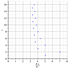
Figure 1: Convergence of $\{\frac{\#+}{\#-}\}$ sequence, $A_{2}$ quiver, $\mu=Id,\mathrm{dim}(M)=i$

$Fset$ matrix arrangement for $A_{4}$ quiver with $d_{i}=4,\mu_{i}=Id$:

$$Fset={\left(\begin{array}[]{cccccccccccccccc}&&x_{1}&x_{2}&&&x_{3}&x_{4}&&&x_{5}&x_{6}&&&x_{7}&x_{8}\\ \vskip 6.0pt plus 2.0pt minus 2.0pt\cr&&x_{1}&x_{11}&&&x_{12}&x_{13}&&&x_{14}&x_{15}&&&x_{16}&x_{17}\\ \vskip 6.0pt plus 2.0pt minus 2.0pt\cr&&1&&&&&&&&&&&&&\\ \vskip 6.0pt plus 2.0pt minus 2.0pt\cr&&&1&&&&&&&&&&&&\\ \vskip 6.0pt plus 2.0pt minus 2.0pt\cr&&&&&&x_{1}&-x_{2}&&&x_{18}&x_{19}&&&x_{2}&x_{21}\\ \vskip 6.0pt plus 2.0pt minus 2.0pt\cr&&&&&&x_{1}&-x_{11}&&&x_{22}&x_{23}&&&x_{24}&x_{25}\\ \vskip 6.0pt plus 2.0pt minus 2.0pt\cr&&&&&&1&&&&&&&&&\\ \vskip 6.0pt plus 2.0pt minus 2.0pt\cr&&&&&&&1&&&&&&&&\\ \vskip 6.0pt plus 2.0pt minus 2.0pt\cr&&&&&&&&&&x_{1}&x_{2}&&&&\\ \vskip 6.0pt plus 2.0pt minus 2.0pt\cr&&&&&&&&&&x_{1}&x_{11}&&&&\\ \vskip 6.0pt plus 2.0pt minus 2.0pt\cr&&&&&&&&&&1&&&&&\\ \vskip 6.0pt plus 2.0pt minus 2.0pt\cr&&&&&&&&&&&1&&&&\\ \vskip 6.0pt plus 2.0pt minus 2.0pt\cr&&&&&&&&&&&&&&x_{1}&-x_{2}\\ \vskip 6.0pt plus 2.0pt minus 2.0pt\cr&&&&&&&&&&&&&&x_{1}&-x_{11}\\ \vskip 6.0pt plus 2.0pt minus 2.0pt\cr&&&&&&&&&&&&&&1&\\ \vskip 6.0pt plus 2.0pt minus 2.0pt\cr&&&&&&&&&&&&&&&1\end{array}\right)}$$ (37)

where $x_{j}=\Delta_{I(j)}$. Compare this to $A_{2},d_{i}=8,\mu_{i}=Id$ case:

$$\tiny{\left(\begin{array}[]{cccccccccccccccc}&&&&x_{{1}}&-x_{{2}}&x_{{3}}&-x_{{4}}&&&&&&&&\\ \vskip 6.0pt plus 2.0pt minus 2.0pt\cr&&&&x_{{5}}&x_{{6}}&x_{{7}}&x_{{8}}&&&&&&&&\\ \vskip 6.0pt plus 2.0pt minus 2.0pt\cr&&&&x_{{9}}&x_{{1}}&x_{{11}}&x_{{12}}&&&&&&&&\\ \vskip 6.0pt plus 2.0pt minus 2.0pt\cr&&&&x_{{13}}&x_{{14}}&x_{{15}}&x_{{16}}&&&&&&&&\\ \vskip 6.0pt plus 2.0pt minus 2.0pt\cr&&&&1&&&&&&&&&&&\\ \vskip 6.0pt plus 2.0pt minus 2.0pt\cr&&&&&1&&&&&&&&&&\\ \vskip 6.0pt plus 2.0pt minus 2.0pt\cr&&&&&&1&&&&&&&&&\\ \vskip 6.0pt plus 2.0pt minus 2.0pt\cr&&&&&&&1&&&&&&&&\\ \vskip 6.0pt plus 2.0pt minus 2.0pt\cr&&&&&&&&&&&&x_{{1}}&x_{{2}}&x_{{3}}&x_{{4}}\\ \vskip 6.0pt plus 2.0pt minus 2.0pt\cr&&&&&&&&&&&&x_{{5}}&-x_{{6}}&x_{{7}}&-x_{{8}}\\ \vskip 6.0pt plus 2.0pt minus 2.0pt\cr&&&&&&&&&&&&x_{{9}}&-x_{{1}}&x_{{11}}&-x_{{12}}\\ \vskip 6.0pt plus 2.0pt minus 2.0pt\cr&&&&&&&&&&&&x_{{13}}&-x_{{14}}&x_{{15}}&-x_{{16}}\\ \vskip 6.0pt plus 2.0pt minus 2.0pt\cr&&&&&&&&&&&&1&&&\\ \vskip 6.0pt plus 2.0pt minus 2.0pt\cr&&&&&&&&&&&&&1&&\\ \vskip 6.0pt plus 2.0pt minus 2.0pt\cr&&&&&&&&&&&&&&1&\\ \vskip 6.0pt plus 2.0pt minus 2.0pt\cr&&&&&&&&&&&&&&&1\end{array}\right)}$$ (38)

Totally positive $Fset$ arrangement for $A_{4}\times{\mathrm{mutations}},d_{i}=6,\mu=Id$:

$$\left(\begin{array}[]{cccccccccccccccccccccccc}&&&1&&1&&&&1&1&1&&&&1&1&1&&&&1&1&1\\ \vskip 6.0pt plus 2.0pt minus 2.0pt\cr&&&1&&1&&&&1&1&1&&&&1&1&1&&&&1&1&1\\ \vskip 6.0pt plus 2.0pt minus 2.0pt\cr&&&1&&1&&&&1&1&1&&&&1&1&1&&&&1&1&1\\ \vskip 6.0pt plus 2.0pt minus 2.0pt\cr&&&1&&&&&&&&&&&&&&&&&&&&\\ \vskip 6.0pt plus 2.0pt minus 2.0pt\cr&&&&1&&&&&&&&&&&&&&&&&&&\\ \vskip 6.0pt plus 2.0pt minus 2.0pt\cr&&&&&1&&&&&&&&&&&&&&&&&&\\ \vskip 6.0pt plus 2.0pt minus 2.0pt\cr&&&&&&&&&1&&1&&&&1&1&1&&&&1&1&1\\ \vskip 6.0pt plus 2.0pt minus 2.0pt\cr&&&&&&&&&1&&1&&&&1&1&1&&&&1&1&1\\ \vskip 6.0pt plus 2.0pt minus 2.0pt\cr&&&&&&&&&1&&1&&&&1&1&1&&&&1&1&1\\ \vskip 6.0pt plus 2.0pt minus 2.0pt\cr&&&&&&&&&1&&&&&&&&&&&&&&\\ \vskip 6.0pt plus 2.0pt minus 2.0pt\cr&&&&&&&&&&1&&&&&&&&&&&&&\\ \vskip 6.0pt plus 2.0pt minus 2.0pt\cr&&&&&&&&&&&1&&&&&&&&&&&&\\ \vskip 6.0pt plus 2.0pt minus 2.0pt\cr&&&&&&&&&&&&&&&1&&1&&&&1&1&1\\ \vskip 6.0pt plus 2.0pt minus 2.0pt\cr&&&&&&&&&&&&&&&1&&1&&&&1&1&1\\ \vskip 6.0pt plus 2.0pt minus 2.0pt\cr&&&&&&&&&&&&&&&1&&1&&&&1&1&1\\ \vskip 6.0pt plus 2.0pt minus 2.0pt\cr&&&&&&&&&&&&&&&1&&&&&&&&\\ \vskip 6.0pt plus 2.0pt minus 2.0pt\cr&&&&&&&&&&&&&&&&1&&&&&&&\\ \vskip 6.0pt plus 2.0pt minus 2.0pt\cr&&&&&&&&&&&&&&&&&1&&&&&&\\ \vskip 6.0pt plus 2.0pt minus 2.0pt\cr&&&&&&&&&&&&&&&&&&&&&1&&1\\ \vskip 6.0pt plus 2.0pt minus 2.0pt\cr&&&&&&&&&&&&&&&&&&&&&1&&1\\ \vskip 6.0pt plus 2.0pt minus 2.0pt\cr&&&&&&&&&&&&&&&&&&&&&1&&1\\ \vskip 6.0pt plus 2.0pt minus 2.0pt\cr&&&&&&&&&&&&&&&&&&&&&1&&\\ \vskip 6.0pt plus 2.0pt minus 2.0pt\cr&&&&&&&&&&&&&&&&&&&&&&1&\\ \vskip 6.0pt plus 2.0pt minus 2.0pt\cr&&&&&&&&&&&&&&&&&&&&&&&1\end{array}\right)$$ (39)

4 •

$$(2,2)= \left(s_{\tiny\yng(2,2)}+s_{\tiny\yng(1,3)}\right)\Delta_{\tiny\yng(2,2)} jsh=\{{\tiny\yng(1)}\}$$ (40)

$$(3,4)= \left(s_{\tiny\yng(2,2,3,3,5,5)}+s_{\tiny\yng(1,1,4,4,5,5)}+s_{\tiny\yng(1,1,3,3,6,6)}\right)\Delta_{\tiny\yng(1,1,3,3,6,6)}+\left(s_{\tiny\yng(1,2,3,3,5,5)}+s_{\tiny\yng(1,1,3,4,5,5)}+s_{\tiny\yng(1,1,3,3,5,6)}\right)\Delta_{\tiny\yng(1,2,3,3,5,5)} jsh=\{{\tiny\yng(1),\yng(1,1)}\}$$

$$(4,6)= \left(s_{\tiny\yng(1,1,2,4,4,4,7,7,7,10,10,10)}+s_{\tiny\yng(1,1,1,4,4,5,7,7,7,10,10,10)}+s_{\tiny\yng(1,1,1,4,4,4,7,7,8,10,10,10)}+s_{\tiny\yng(1,1,1,4,4,4,7,7,7,10,10,11)}\right)\Delta_{\tiny\yng(1,1,1,4,4,5,7,7,7,10,10,10)}+\left(s_{\tiny\yng(1,1,1,4,4,7,7,7,7,10,10,10)}+s_{\tiny\yng(1,1,1,4,4,4,7,7,7,10,10,13)}+s_{\tiny\yng(1,1,1,4,4,4,7,7,10,10,10,10)}+s_{\tiny\yng(1,1,4,4,4,4,7,7,7,10,10,10)}\right)\Delta_{\tiny\yng(1,1,1,4,4,7,7,7,7,10,10,10)}+$$

$$\left(s_{\tiny\yng(1,2,2,4,4,4,7,7,7,10,10,10)}+s_{\tiny\yng(1,1,1,4,4,4,7,7,7,10,11,11)}+s_{\tiny\yng(1,1,1,4,5,5,7,7,7,10,10,10)}+s_{\tiny\yng(1,1,1,4,4,4,7,8,8,10,10,10)}\right)\Delta_{\tiny\yng(1,1,1,4,5,5,7,7,7,10,10,10)}+\left(s_{\tiny\yng(1,1,1,4,4,4,7,8,10,10,10,10)}+s_{\tiny\yng(1,2,4,4,4,4,7,7,7,10,10,10)}+s_{\tiny\yng(1,1,1,4,5,7,7,7,7,10,10,10)}+s_{\tiny\yng(1,1,1,4,4,4,7,7,7,10,11,13)}\right)\Delta_{\tiny\yng(1,1,1,4,5,7,7,7,7,10,10,10)}+$$

$$\left(s_{\tiny\yng(2,2,2,4,4,4,7,7,7,10,10,10)}+s_{\tiny\yng(1,1,1,4,4,4,8,8,8,10,10,10)}+s_{\tiny\yng(1,1,1,5,5,5,7,7,7,10,10,10)}+s_{\tiny\yng(1,1,1,4,4,4,7,7,7,11,11,11)}\right)\Delta_{\tiny\yng(1,1,1,5,5,5,7,7,7,10,10,10)}+\left(s_{\tiny\yng(2,2,4,4,4,4,7,7,7,10,10,10)}+s_{\tiny\yng(1,1,1,5,5,7,7,7,7,10,10,10)}+s_{\tiny\yng(1,1,1,4,4,4,7,7,7,11,11,13)}+s_{\tiny\yng(1,1,1,4,4,4,8,8,10,10,10,10)}\right)\Delta_{\tiny\yng(1,1,1,5,5,7,7,7,7,10,10,10)} jsh=\{{\tiny\yng(1),\yng(1,1),\yng(1,3),\yng(3),\yng(1,1,1),\yng(1,1,3)}\}$$

$$(5,8)= \left(s_{\tiny\yng(1,1,1,1,5,5,5,5,9,9,9,10,13,13,13,13,17,17,17,17)}+s_{\tiny\yng(1,1,1,2,5,5,5,5,9,9,9,9,13,13,13,13,17,17,17,17)}+s_{\tiny\yng(1,1,1,1,5,5,5,6,9,9,9,9,13,13,13,13,17,17,17,17)}+s_{\tiny\yng(1,1,1,1,5,5,5,5,9,9,9,9,13,13,13,14,17,17,17,17)}+s_{\tiny\yng(1,1,1,1,5,5,5,5,9,9,9,9,13,13,13,13,17,17,17,18)}\right)\Delta_{\tiny\yng(1,1,1,1,5,5,5,5,9,9,9,9,13,13,13,14,17,17,17,17)}+\dots jsh=\{{\tiny\yng(1),\yng(1,1),\dots,\yng(1,1,1,1),\yng(1,1,1,3)}\}$$

(1,1,1,2,2,5,7,7,7,7,7,7,13,13,13,13,13,13,19,19,19,19,19,19,25,25,25,25,25,25,31,31,31,31,31,31,37,37,37,37,37,37,43,43,43,43,43,43,49,49,49,49,49,49,55,55,55,55,55,55,61,61,61,61,61,61,67,67,67,67,67,67)

$\frac{1}{2}(\tilde{P}_{+}-\tilde{P}_{-})$ for cyclic 6-vertex graph:

$$\left(-s_{\tiny\yng(1,1,1,4,4,4,7,7,7,10,10,10,13,13,16,16,16,16)}+s_{\tiny\yng(1,1,1,4,4,4,7,7,7,10,10,13,13,13,13,16,16,16)}\right)\Delta_{\tiny\yng(1,1,1,4,4,4,7,7,7,10,10,13,13,13,13,16,16,16)}+\left(s_{\tiny\yng(1,1,1,4,4,4,7,7,7,10,11,13,13,13,13,16,16,16)}-s_{\tiny\yng(1,1,1,4,4,4,7,7,7,10,10,10,13,14,16,16,16,16)}\right)\Delta_{\tiny\yng(1,1,1,4,4,4,7,7,7,10,11,13,13,13,13,16,16,16)}+\left(-s_{\tiny\yng(1,1,1,4,4,4,7,7,7,10,10,10,14,14,16,16,16,16)}+s_{\tiny\yng(1,1,1,4,4,4,7,7,7,11,11,13,13,13,13,16,16,16)}\right)\Delta_{\tiny\yng(1,1,1,4,4,4,7,7,7,11,11,13,13,13,13,16,16,16)}$$ (41)

Lemma 1. Asymptotic formula for $\tilde{P}_{\mathrm{max}}(Q_{\mathrm{univ}}(n),n,Id)$:

• $m\times m$ ‘‘cubic ladder’’ decomposition $\simeq\Delta$-summands in $\tilde{P_{I}}$

• each $\Delta$-summand consists of Young diagrams factorized by the ‘‘ladder-block’’ addition

The formula:

$$\boxed{\tilde{P}_{\mathrm{max}}(Q(m),n,Id)=\sum\limits_{i=1..m\cdot\mathrm{cl}\left(\frac{m}{2}\right)}\sum\limits_{j=1..n}s_{\lambda(i,j)}\Delta_{\lambda(i,*)},}$$ (42)

$\frac{1}{2}(\tilde{P}_{+}-\tilde{P}_{-})$ for cyclic 8-vertex graph:

$$\left(-s_{\tiny\yng(1,1,1,1,5,5,5,5,9,9,9,9,13,13,13,13,18,18,18,20,21,21,21,21,25,25,25,25,29,29,29,29)}+s_{\tiny\yng(1,1,1,1,5,5,5,5,9,9,9,9,13,13,13,13,17,17,17,17,22,22,22,24,25,25,25,25,29,29,29,29)}\right)\Delta_{\tiny\yng(1,1,1,1,5,5,5,5,9,9,9,9,13,13,13,15,17,17,17,17,21,21,21,21,25,25,25,25,29,29,29,29)}+\left(s_{\tiny\yng(1,1,1,1,5,5,5,5,9,9,9,9,13,13,13,13,17,17,17,17,21,21,21,21,26,26,26,28,29,29,29,29)}-s_{\tiny\yng(1,1,1,1,5,5,5,5,9,9,9,9,13,13,13,13,18,18,18,18,21,21,21,21,25,25,25,25,29,29,29,29)}\right)\Delta_{\tiny\yng(1,1,1,1,5,5,5,5,9,9,9,9,13,13,13,17,17,17,17,17,21,21,21,21,25,25,25,25,29,29,29,29)}+\left(s_{\tiny\yng(1,1,1,1,5,5,5,5,9,9,9,9,13,13,13,13,17,17,17,17,21,21,21,24,25,25,25,25,29,29,29,29)}-s_{\tiny\yng(1,1,1,1,5,5,5,5,9,9,9,9,13,13,13,13,17,17,17,20,21,21,21,21,25,25,25,25,29,29,29,29)}\right)\Delta_{\tiny\yng(1,1,1,1,5,5,5,5,9,9,9,9,13,13,14,15,17,17,17,17,21,21,21,21,25,25,25,25,29,29,29,29)}+\left(s_{\tiny\yng(1,1,1,1,5,5,5,5,9,9,9,9,13,13,13,13,17,17,17,17,21,21,21,21,25,25,25,28,29,29,29,29)}-s_{\tiny\yng(1,1,1,1,5,5,5,5,9,9,9,9,13,13,13,13,17,17,17,18,21,21,21,21,25,25,25,25,29,29,29,29)}\right)\Delta_{\tiny\yng(1,1,1,1,5,5,5,5,9,9,9,9,13,13,14,17,17,17,17,17,21,21,21,21,25,25,25,25,29,29,29,29)}+$$ (43)

$$\left(s_{\tiny\yng(1,1,1,1,5,5,5,5,9,9,9,9,13,13,13,13,17,17,17,17,21,21,22,24,25,25,25,25,29,29,29,29)}-s_{\tiny\yng(1,1,1,1,5,5,5,5,9,9,9,9,13,13,13,13,17,17,18,20,21,21,21,21,25,25,25,25,29,29,29,29)}\right)\Delta_{\tiny\yng(1,1,1,1,5,5,5,5,9,9,9,9,13,14,14,15,17,17,17,17,21,21,21,21,25,25,25,25,29,29,29,29)}+\left(s_{\tiny\yng(1,1,1,1,5,5,5,5,9,9,9,9,13,13,13,13,17,17,17,17,21,21,21,21,25,25,26,28,29,29,29,29)}-s_{\tiny\yng(1,1,1,1,5,5,5,5,9,9,9,9,13,13,13,13,17,17,18,18,21,21,21,21,25,25,25,25,29,29,29,29)}\right)\Delta_{\tiny\yng(1,1,1,1,5,5,5,5,9,9,9,9,13,14,14,17,17,17,17,17,21,21,21,21,25,25,25,25,29,29,29,29)}+\left(s_{\tiny\yng(1,1,1,1,5,5,5,5,9,9,9,9,13,13,13,13,17,17,17,17,21,22,22,24,25,25,25,25,29,29,29,29)}-s_{\tiny\yng(1,1,1,1,5,5,5,5,9,9,9,9,13,13,13,13,17,18,18,20,21,21,21,21,25,25,25,25,29,29,29,29)}\right)\Delta_{\tiny\yng(1,1,1,1,5,5,5,5,9,9,9,9,14,14,14,15,17,17,17,17,21,21,21,21,25,25,25,25,29,29,29,29)}+\left(s_{\tiny\yng(1,1,1,1,5,5,5,5,9,9,9,9,13,13,13,13,17,17,17,17,21,21,21,21,25,26,26,28,29,29,29,29)}-s_{\tiny\yng(1,1,1,1,5,5,5,5,9,9,9,9,13,13,13,13,17,18,18,18,21,21,21,21,25,25,25,25,29,29,29,29)}\right)\Delta_{\tiny\yng(1,1,1,1,5,5,5,5,9,9,9,9,14,14,14,17,17,17,17,17,21,21,21,21,25,25,25,25,29,29,29,29)}$$

5 Re-evaluation of $\tilde{P}$ for Coxeter quivers. ‘‘Vertex at $\infty$’’

Let $Q$ be a quiver with $m$ vertices and all possible arrows (but only 2 opposite arrows for each pair of vertices is allowed, so the direction $v=\pm 1$) . Choose $n,e\in\mathbb{N}$ and the integer-valued vectors

$$B=\{1,\dots,m\cdot{}n\},I=\{jn-i+1\}_{i=1..[n/2],j=1..m}\subset B,|I|=e,$$ (44)

where $[x]\text{ is the integer part of }x$. Fix the representation $R(Q)$: vertices $\sim V_{i}(\mathbb{Z}^{n})$, arrows $\sim$ transposition matrices $M_{v,i,j}=\sigma(\lambda_{i,j})^{\mathrm{sign}(v)}$.

Each $\sigma(\lambda_{i,j})$ is a $(n\times n)$ transposition matrix, partitioned by $\lambda_{i,j}$ for the $(i,j)$-th arrow. We fix the particular choice $\boxed{R=\Sigma_{0}}$:

$$(i,j)\rightarrow\lambda_{i,j}:(1,4)\rightarrow{\tiny\yng(1,2,3,4)},(1,3)\rightarrow{\tiny\yng(1,2,3,3)},(1,2)\rightarrow{\tiny\yng(1,2,2,2)},(2,4)\rightarrow{\tiny\yng(2,2,3,4)},(2,3)\rightarrow{\tiny\yng(2,2,3,3)},\dots$$ (45)

Assume also $\mathrm{dim(Gr}(Q,R))=\boxed{\overline{e}=\left[\frac{1}{2}\overline{n}\right]}$ for the corresponding quiver grassmannian [2, 4], $e_{i}=e_{j}\ \forall i,j$. For instance, the case $(m,n)=(4,4)$ is given by

$$\mathbf{M}_{+}={\tiny\left(\begin{array}[]{cccc}0&\left[\begin{array}[]{cccc}1&0&0&0\\ \vskip 6.0pt plus 2.0pt minus 2.0pt\cr 0&0&1&0\\ \vskip 6.0pt plus 2.0pt minus 2.0pt\cr 0&0&0&1\\ \vskip 6.0pt plus 2.0pt minus 2.0pt\cr 0&1&0&0\end{array}\right]&\left[\begin{array}[]{cccc}1&0&0&0\\ \vskip 6.0pt plus 2.0pt minus 2.0pt\cr 0&1&0&0\\ \vskip 6.0pt plus 2.0pt minus 2.0pt\cr 0&0&0&1\\ \vskip 6.0pt plus 2.0pt minus 2.0pt\cr 0&0&1&0\end{array}\right]&\left[\begin{array}[]{cccc}1&0&0&0\\ \vskip 6.0pt plus 2.0pt minus 2.0pt\cr 0&1&0&0\\ \vskip 6.0pt plus 2.0pt minus 2.0pt\cr 0&0&1&0\\ \vskip 6.0pt plus 2.0pt minus 2.0pt\cr 0&0&0&1\end{array}\right]\\ \vskip 6.0pt plus 2.0pt minus 2.0pt\cr 0&0&\left[\begin{array}[]{cccc}0&1&0&0\\ \vskip 6.0pt plus 2.0pt minus 2.0pt\cr 1&0&0&0\\ \vskip 6.0pt plus 2.0pt minus 2.0pt\cr 0&0&0&1\\ \vskip 6.0pt plus 2.0pt minus 2.0pt\cr 0&0&1&0\end{array}\right]&\left[\begin{array}[]{cccc}0&1&0&0\\ \vskip 6.0pt plus 2.0pt minus 2.0pt\cr 1&0&0&0\\ \vskip 6.0pt plus 2.0pt minus 2.0pt\cr 0&0&1&0\\ \vskip 6.0pt plus 2.0pt minus 2.0pt\cr 0&0&0&1\end{array}\right]\\ \vskip 6.0pt plus 2.0pt minus 2.0pt\cr 0&0&0&\left[\begin{array}[]{cccc}0&1&0&0\\ \vskip 6.0pt plus 2.0pt minus 2.0pt\cr 0&0&1&0\\ \vskip 6.0pt plus 2.0pt minus 2.0pt\cr 1&0&0&0\\ \vskip 6.0pt plus 2.0pt minus 2.0pt\cr 0&0&0&1\end{array}\right]\\ \vskip 6.0pt plus 2.0pt minus 2.0pt\cr 0&0&0&0\end{array}\right)}$$ (46)

and $\mathbf{M}_{-}$ equals by-block inverse of $\mathbf{M}_{+}$. Choose some path $x\in\mathcal{P}(Q)$ and solve the quiver relations with vanishing conditions [4]:

$$\sum_{s^{\prime},t^{\prime}}(-1)_{\epsilon(s^{\prime},t^{\prime})}M_{v,s^{\prime},t^{\prime}}\ \Delta_{s}^{s^{\prime}}\ \Delta_{t^{\prime}}^{t}-\ \sum_{s^{\prime}}(-1)_{\epsilon(s^{\prime},t)}M_{v,s^{\prime},t}\ \Delta_{s}^{s^{\prime}}\ \Delta_{I}=0,$$ (47)

$$\Delta_{J}=0\text{ for some non-proper }J\text{'s}$$

Define symmetric polynomials

$$\boxed{\tilde{P}_{R}(x)=\sum\limits_{i,j}\Delta_{\mu_{i,i}}s_{\mu_{i,j}}(p_{1},p_{2},\dots)},$$ (48)

where $\mu_{i,j}$ is a partition derived from the Cauchy-Binet expansion for each $\Delta$’s, $s_{\mu}$ is a Schur function.

Prop 1. The map $f:x\mapsto\tilde{P}_{R}(x)$ is a homomorphism on a ‘‘proper’’ subset $S\subseteq\mathcal{P}$, s.t. for any $x,y\in S$

$$\tilde{P}_{R}(x\cdot y)=\frac{1}{2}\sum_{\mu,\eta,\nu}\left(\mathrm{coeff}(\tilde{P}_{R}(x),\Delta_{\mu})-\mathrm{coeff}(\tilde{P}_{R}(y),\Delta_{\eta})\right)\Delta_{\nu}\simeq_{|_{Res(\Delta)}}\frac{1}{2}\left(\tilde{P}_{R}(x)-\tilde{P}_{R}(y)\right)$$ (49)

Note: this construction is very sensitive to the choice of $R$ (if we swap the transposition matrices, $S$ will change).

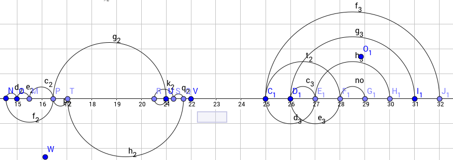
Figure 2: Examples of ‘‘good’’ (left) and ‘‘bad’’ (right) combinations of paths in $S\subseteq\mathcal{P}$ for $(m,n)=(10,10)$. ‘‘Good’’ means the image of $f$ is not empty

Figure 3: Examples of a non-trivial loops spiral type 1 (Coxeter odd type $\tilde{A}_{n}$) for $(m,n)=(6,6),(8,8),(10,10),\dots$

Lemma 2. If $x\in\mathcal{P}(Q)$ is of spiral type 1, then

$$\tilde{P}_{\pm}(x)\equiv 0,$$ (50)

where ‘‘$\pm$’’ means that we take a doubled path with $v=\pm 1$. This lemma can be improved if we take all irreducible subsets of the set of all arrows of $Q$, on which our polynomial vanishes. For instance, each minimal null-set for $4$-vertex quiver is trivial, $6$-vertex: $\{(1,6),(3,4),(1,5),(3,6)\}$ - is not minimal, but irreducible (recall that in this case orientation does not matter), $8$-vertex: $\{(2,7),(3,6),(2,6),(3,5)\}$, $12$-vertex: $\{(5,8),(3,10),(4,9),(4,8),(5,7),(3,9)\}$ and so on. Let’s write the corresponding symmetric polynomials explicitly:

$$\hat{P}_{i}=\left.\frac{\tilde{P}_{+}(x_{i})-\tilde{P}_{-}(x_{i})}{2}\right|_{\lambda_{j,k}\mapsto\mathcal{Y}(\lambda_{j,k})},\quad\mathcal{Y}(l_{i})=\emptyset,\mathcal{Y}(\lambda>l_{i})=[\lambda-l_{i}]$$ (51)

$$\hat{P}_{4}= 0$$ (52)

$$\hat{P}_{6}= \left(s_{\tiny\yng(1,1,3)_{2}}-s_{\tiny\yng(1,1,3)_{1}}\right)\Delta_{\tiny\yng(2)_{3}}+\left(s_{\tiny\yng(3)_{2}}-s_{\tiny\yng(3)_{1}}\right)\Delta_{\tiny\yng(1,2)_{3}}+\left(s_{\tiny\yng(1,3)_{2}}-s_{\tiny\yng(1,3)_{1}}\right)\Delta_{\tiny\yng(1,1,2)_{3}}$$

$$\hat{P}_{8}= \left(s_{\tiny\yng(1,1,1,3)_{3}}-s_{\tiny\yng(1,1,1,3)_{2}}\right)\Delta_{\tiny\yng(2)_{4}}+\left(s_{\tiny\yng(1,1,1,1)_{3}}-s_{\tiny\yng(1,1,1,3)_{1}}\right)\Delta_{\tiny\yng(4)_{4}}+\left(-s_{\tiny\yng(3)_{2}}+s_{\tiny\yng(3)_{3}}\right)\Delta_{\tiny\yng(1,2)_{4}}+$$

$$+\left(s_{\tiny\yng(1)_{3}}-s_{\tiny\yng(3)_{1}}\right)\Delta_{\tiny\yng(1,4)_{4}}+\left(-s_{\tiny\yng(1,3)_{2}}+s_{\tiny\yng(1,3)_{3}}\right)\Delta_{\tiny\yng(1,1,2)_{4}}+\left(s_{\tiny\yng(1,1)_{3}}-s_{\tiny\yng(1,3)_{1}}\right)\Delta_{\tiny\yng(1,1,4)_{4}}+$$

$$+\left(s_{\tiny\yng(1,1,3)_{3}}-s_{\tiny\yng(1,1,3)_{2}}\right)\Delta_{\tiny\yng(1,1,1,2)_{4}}+\left(s_{\tiny\yng(1,1,1)_{3}}-s_{\tiny\yng(1,1,3)_{1}}\right)\Delta_{\tiny\yng(1,1,1,4)_{4}}$$

$$\hat{P}_{10}= \left(-s_{\tiny\yng(3)_{3}}+s_{\tiny\yng(3)_{4}}\right)\Delta_{\tiny\yng(2)_{9}}+\left(-s_{\tiny\yng(5)_{1}}+s_{\tiny\yng(5)_{2}}+s_{\tiny\yng(5)_{4}}-s_{\tiny\yng(5)_{3}}\right)\Delta_{\tiny\yng(4)_{9}}+$$

$$+\left(s_{\tiny\yng(4)_{1}}-s_{\tiny\yng(2)_{3}}\right)\Delta_{\tiny\yng(5)_{9}}+\left(-s_{\tiny\yng(1,3)_{3}}+s_{\tiny\yng(1,3)_{4}}\right)\Delta_{\tiny\yng(1,2)_{9}}+\left(s_{\tiny\yng(1,5)_{2}}-s_{\tiny\yng(1,5)_{3}}-\right.$$

$$\left.-s_{\tiny\yng(1,5)_{1}}+s_{\tiny\yng(1,5)_{4}}\right)\Delta_{\tiny\yng(1,4)_{9}}+\left(s_{\tiny\yng(1,4)_{1}}-s_{\tiny\yng(1,2)_{3}}\right)\Delta_{\tiny\yng(1,5)_{9}}+\left(s_{\tiny\yng(1,1,3)_{4}}-s_{\tiny\yng(1,1,3)_{3}}\right)\Delta_{\tiny\yng(1,1,2)_{9}}+$$

$$+\left(-s_{\tiny\yng(1,1,5)_{3}}+s_{\tiny\yng(1,1,5)_{2}}+s_{\tiny\yng(1,1,5)_{4}}-s_{\tiny\yng(1,1,5)_{1}}\right)\Delta_{\tiny\yng(1,1,4)_{9}}+\left(s_{\tiny\yng(1,1,4)_{1}}-s_{\tiny\yng(1,1,2)_{3}}\right)\Delta_{\tiny\yng(1,1,5)_{9}}+$$

$$+\left(-s_{\tiny\yng(1,1,1,3)_{3}}+s_{\tiny\yng(1,1,1,3)_{4}}\right)\Delta_{\tiny\yng(1,1,1,2)_{9}}\left(-s_{\tiny\yng(1,1,1,5)_{1}}+s_{\tiny\yng(1,1,1,5)_{4}}-s_{\tiny\yng(1,1,1,5)_{3}}+s_{\tiny\yng(1,1,1,5)_{2}}\right)\Delta_{\tiny\yng(1,1,1,4)_{9}}+$$

$$+\left(s_{\tiny\yng(1,1,1,4)_{1}}-s_{\tiny\yng(1,1,1,2)_{3}}\right)\Delta_{\tiny\yng(1,1,1,5)_{9}}+\left(s_{\tiny\yng(1,1,1,1,3)_{4}}-s_{\tiny\yng(1,1,1,1,3)_{3}}\right)\Delta_{\tiny\yng(1,1,1,1,2)_{9}}+$$

$$+\left(s_{\tiny\yng(1,1,1,1,5)_{4}}+s_{\tiny\yng(1,1,1,1,5)_{2}}-s_{\tiny\yng(1,1,1,1,5)_{3}}-s_{\tiny\yng(1,1,1,1,5)_{1}}\right)\Delta_{\tiny\yng(1,1,1,1,4)_{9}}+\left(s_{\tiny\yng(1,1,1,1,4)_{1}}-s_{\tiny\yng(1,1,1,1,2)_{3}}\right)\Delta_{\tiny\yng(1,1,1,1,5)_{9}}$$

$$\hat{P}_{12}= \left(s_{\tiny\yng(3)_{5}}-s_{\tiny\yng(3)_{4}}\right)\Delta_{\tiny\yng(2)_{11}}+\left(s_{\tiny\yng(5)_{3}}-s_{\tiny\yng(5)_{4}}+s_{\tiny\yng(5)_{5}}-s_{\tiny\yng(5)_{2}}\right)\Delta_{\tiny\yng(4)_{11}}+\left(s_{\tiny\yng(1,3)_{5}}-s_{\tiny\yng(1,3)_{4}}\right)\Delta_{\tiny\yng(1,2)_{11}}+$$

$$+\left(s_{\tiny\yng(1,5)_{5}}-s_{\tiny\yng(1,5)_{2}}+s_{\tiny\yng(1,5)_{3}}-s_{\tiny\yng(1,5)_{4}}\right)\Delta_{\tiny\yng(1,4)_{11}}+\left(-s_{\tiny\yng(1,1,3)_{4}}+s_{\tiny\yng(1,1,3)_{5}}\right)\Delta_{\tiny\yng(1,1,2)_{11}}+$$

$$+\left(-s_{\tiny\yng(1,1,5)_{4}}-s_{\tiny\yng(1,1,5)_{2}}+s_{\tiny\yng(1,1,5)_{5}}+s_{\tiny\yng(1,1,5)_{3}}\right)\Delta_{\tiny\yng(1,1,4)_{11}}+\left(-s_{\tiny\yng(1,1,1,3)_{4}}+s_{\tiny\yng(1,1,1,3)_{5}}\right)\Delta_{\tiny\yng(1,1,1,2)_{11}}+$$

$$+\left(-s_{\tiny\yng(1,1,1,1,5)_{4}}+s_{\tiny\yng(1,1,1,1,5)_{5}}+s_{\tiny\yng(1,1,1,1,5)_{3}}-s_{\tiny\yng(1,1,1,1,5)_{2}}\right)\Delta_{\tiny\yng(1,1,1,1,4)_{11}}+\left(s_{\tiny\yng(1,1,1,1,1,3)_{5}}-s_{\tiny\yng(1,1,1,1,1,3)_{4}}\right)\Delta_{\tiny\yng(1,1,1,1,1,2)_{11}}+$$

$$+\left(-s_{\tiny\yng(1,1,1,1,1,5)_{2}}-s_{\tiny\yng(1,1,1,1,1,5)_{4}}+s_{\tiny\yng(1,1,1,1,1,5)_{5}}+s_{\tiny\yng(1,1,1,1,1,5)_{3}}\right)\Delta_{\tiny\yng(1,1,1,1,1,4)_{11}}+\dots$$

Another (stand-alone) example:

$$-I\hat{P}_{6}(spiral_{2})=s_{\tiny\yng(1,1,2)_{2}}+s_{\tiny\yng(1,2)_{0}}+s_{\tiny\yng(1,1,2)_{4}}-s_{\tiny\yng(1,1,2)_{3}}-s_{\tiny\yng(1,2)_{5}}-s_{\tiny\yng(2)_{1}}$$ (53)

Let $(m,n)=(6,6)$; consider the following two paths and their concatenation:

$$\tilde{P}(Q_{1})= \left(s_{\tiny\yng(1)_{0}}+s_{\tiny\yng(1,1)_{3}}+s_{\tiny\yng(1)_{5}}+s_{\tiny\yng(2)_{2}}\right)\Delta_{\tiny\yng(1)_{5}}+\left(-s_{\tiny\yng(2)_{0}}+s_{\tiny\yng(1,2)_{3}}+s_{\tiny\yng(2)_{5}}-s_{\tiny\yng(3)_{2}}\right)\Delta_{\tiny\yng(2)_{5}}+$$ (54)

$$+\left(s_{\tiny\yng(1)_{2}}+s_{\tiny\yng(3)_{0}}+s_{\tiny\yng(3)_{5}}+s_{\tiny\yng(1,3)_{3}}\right)\Delta_{\tiny\yng(3)_{5}}+\left(s_{\tiny\yng(1,1)_{5}}+s_{\tiny\yng(1,1)_{0}}+s_{\tiny\yng(1,1,1)_{3}}+s_{\tiny\yng(1,2)_{2}}\right)\Delta_{\tiny\yng(1,1)_{5}}+$$

$$+\left(-s_{\tiny\yng(1,3)_{2}}+s_{\tiny\yng(1,1,2)_{3}}+s_{\tiny\yng(1,2)_{5}}-s_{\tiny\yng(1,2)_{0}}\right)\Delta_{\tiny\yng(1,2)_{5}}+\left(s_{\tiny\yng(1,3)_{0}}+s_{\tiny\yng(1,1)_{2}}+s_{\tiny\yng(1,3)_{5}}+s_{\tiny\yng(1,1,3)_{3}}\right)\Delta_{\tiny\yng(1,3)_{5}}+$$

$$+\left(s_{\tiny\yng(1,1,1)_{5}}+s_{\tiny\yng(1,1,2)_{2}}+s_{\tiny\yng(1,1,1)_{0}}+s_{\tiny\yng(1)_{3}}\right)\Delta_{\tiny\yng(1,1,1)_{5}}+\left(s_{\tiny\yng(2)_{3}}-s_{\tiny\yng(1,1,3)_{2}}+s_{\tiny\yng(1,1,2)_{5}}-s_{\tiny\yng(1,1,2)_{0}}\right)\Delta_{\tiny\yng(1,1,2)_{5}}+$$

$$+\left(s_{\tiny\yng(1,1,3)_{5}}+s_{\tiny\yng(3)_{3}}+s_{\tiny\yng(1,1,1)_{2}}+s_{\tiny\yng(1,1,3)_{0}}\right)\Delta_{\tiny\yng(1,1,3)_{5}}\quad\text{\# 5 is the longest arc}$$

$$\tilde{P}(Q_{2})= \left(s_{\tiny\yng(1)_{4}}+s_{\tiny\yng(1)_{5}}-s_{\tiny\yng(2)_{2}}+s_{\tiny\yng(1)_{1}}\right)\Delta_{\tiny\yng(1)_{4}}+\left(-s_{\tiny\yng(2)_{5}}-s_{\tiny\yng(3)_{1}}+s_{\tiny\yng(3)_{2}}+s_{\tiny\yng(2)_{4}}\right)\Delta_{\tiny\yng(2)_{4}}+$$

$$+\left(-s_{\tiny\yng(3)_{5}}+s_{\tiny\yng(1)_{2}}+s_{\tiny\yng(3)_{4}}+s_{\tiny\yng(2)_{1}}\right)\Delta_{\tiny\yng(3)_{4}}+\left(-s_{\tiny\yng(1,1,2)_{2}}+s_{\tiny\yng(1,1,1)_{1}}+s_{\tiny\yng(1,1)_{4}}+s_{\tiny\yng(1,1,1)_{5}}\right)\Delta_{\tiny\yng(1,1)_{4}}+$$

$$+\left(-s_{\tiny\yng(1,1,2)_{5}}+s_{\tiny\yng(1,1,3)_{2}}+s_{\tiny\yng(1,2)_{4}}-s_{\tiny\yng(1,1,3)_{1}}\right)\Delta_{\tiny\yng(1,2)_{4}}+\left(s_{\tiny\yng(1,1,1)_{2}}-s_{\tiny\yng(1,1,3)_{5}}+s_{\tiny\yng(1,1,2)_{1}}+s_{\tiny\yng(1,3)_{4}}\right)\Delta_{\tiny\yng(1,3)_{4}}+$$

$$+\left(s_{\tiny\yng(1,1)_{1}}+s_{\tiny\yng(1,1)_{5}}+s_{\tiny\yng(1,1,1)_{4}}-s_{\tiny\yng(1,2)_{2}}\right)\Delta_{\tiny\yng(1,1,1)_{4}}+\left(-s_{\tiny\yng(1,3)_{1}}-s_{\tiny\yng(1,2)_{5}}+s_{\tiny\yng(1,1,2)_{4}}+s_{\tiny\yng(1,3)_{2}}\right)\Delta_{\tiny\yng(1,1,2)_{4}}+$$

$$+\left(s_{\tiny\yng(1,1)_{2}}+s_{\tiny\yng(1,2)_{1}}+s_{\tiny\yng(1,1,3)_{4}}-s_{\tiny\yng(1,3)_{5}}\right)\Delta_{\tiny\yng(1,1,3)_{4}}\quad\text{\# 4 is the longest arc}$$

$$\tilde{P}(Q_{1,2})= \left(-s_{\tiny\yng(1,1,3)_{2}}+s_{\tiny\yng(1,1,3)_{1}}-s_{\tiny\yng(1,2)_{4}}-s_{\tiny\yng(1,1,2)_{0}}+s_{\tiny\yng(2)_{3}}+s_{\tiny\yng(1,1,2)_{5}}\right)\Delta_{\tiny\yng(2)_{3}}+\left(s_{\tiny\yng(2)_{5}}+s_{\tiny\yng(3)_{1}}-s_{\tiny\yng(3)_{2}}-s_{\tiny\yng(2)_{4}}-s_{\tiny\yng(2)_{0}}+s_{\tiny\yng(1,2)_{3}}\right)\Delta_{\tiny\yng(1,2)_{3}}+$$

$$+\left(s_{\tiny\yng(1,2)_{5}}-s_{\tiny\yng(1,2)_{0}}-s_{\tiny\yng(1,1,2)_{4}}+s_{\tiny\yng(1,1,2)_{3}}+s_{\tiny\yng(1,3)_{1}}-s_{\tiny\yng(1,3)_{2}}\right)\Delta_{\tiny\yng(1,1,2)_{3}}=$$

$$= \frac{1}{2}\left(\mathrm{coeff}(P(Q_{1}),\Delta_{\tiny\yng(1,1,2)_{5}})-\mathrm{coeff}(P(Q_{2}),\Delta_{\tiny\yng(1,2)_{4}})\right)\Delta_{\tiny\yng(2)_{3}}+\frac{1}{2}\left(\mathrm{coeff}(P(Q_{1}),\Delta_{\tiny\yng(2)_{5}})-\mathrm{coeff}(P(Q_{2}),\Delta_{\tiny\yng(2)_{4}})\right)\Delta_{\tiny\yng(1,2)_{3}}+$$

$$+\frac{1}{2}\left(\mathrm{coeff}(P(Q_{1}),\Delta_{\tiny\yng(1,2)_{5}})-\mathrm{coeff}(P(Q_{2}),\Delta_{\tiny\yng(1,1,2)_{4}})\right)\Delta_{\tiny\yng(1,1,2)_{3}}=\frac{1}{2}\left(P(Q_{1})-\mathrm{permut}(P(Q_{2}),\Delta_{*})\right)$$

(This is a particular example related to the proposition 1).

The next goal is to build infinite series like this

$$Z_{R}(S)=\frac{1}{2k}\sum\limits_{i,j}\left(\tilde{P}_{R}(x_{i})-\tilde{P}_{R}(x_{j})\right),$$ (55)

where $S=\{x_{1},x_{2},\dots,x_{i},\dots\}\subseteq\mathcal{P}(Q_{n\to\infty})\ \text{ is a proper union of loops}$.

Figure 4: Concatenation of $x_{i}\in S$ for $R=\Sigma_{0}$

Of course it can be rewritten in terms of Schur function expansion

$$Z_{R}(S)=\sum\limits_{\lambda}g_{\lambda}(\Delta)s_{\lambda}(p_{1},p_{2},\dots),$$ (56)

or, in our ‘‘ladder notation’’, over all $\Gamma$-type weighted Young diagrams, using the $\mathcal{Y}$ operator

$$Z_{R}(S)=\sum\limits_{\lambda_{w}}g_{\lambda_{w}}(\Delta)\tilde{s}_{\lambda_{w}}(p_{1},p_{2},\dots),\quad w\in\mathbb{N},\quad\lambda_{w}=\mathcal{Y}(\lambda)$$ (57)

Take $S^{\prime}=\{x_{1},x_{2}\}\subset\mathcal{P}(Q_{10}),(m,n)=(10,10)$. In this case the double-path polynomial is non-trivial (!)

$$\tilde{P}_{\pm}(S^{\prime})= \left(s_{\tiny\yng(1)_{2}}+s_{\tiny\yng(1,5)_{8}}+s_{\tiny\yng(1)_{6}}+s_{\tiny\yng(1)_{3}}+s_{\tiny\yng(1,5)_{9}}+s_{\tiny\yng(1)_{1}}+s_{\tiny\yng(1)_{7}}+s_{\tiny\yng(1,1)_{5}}+s_{\tiny\yng(1,1)_{4}}\right)\Delta_{\tiny\yng(1)_{6}}+$$ (58)

$$+\left(s_{\tiny\yng(1,1)_{3}}+s_{\tiny\yng(1,1)_{2}}+s_{\tiny\yng(1,1,1)_{5}}+s_{\tiny\yng(1,1)_{1}}+s_{\tiny\yng(1,1,5)_{8}}+s_{\tiny\yng(1,1,1)_{4}}+s_{\tiny\yng(1,1,1)_{6}}+s_{\tiny\yng(1,1)_{7}}+s_{\tiny\yng(1,1,5)_{9}}\right)\Delta_{\tiny\yng(1,1,1)_{6}}+$$

$$+\left(s_{\tiny\yng(1,1,1,1)_{5}}+s_{\tiny\yng(1,1,1,1)_{6}}+s_{\tiny\yng(1,1,1)_{2}}+s_{\tiny\yng(1,1,1,1)_{4}}+s_{\tiny\yng(1,1,1)_{3}}+s_{\tiny\yng(1,1,1,5)_{9}}+s_{\tiny\yng(1,1,1,1,5)_{8}}+s_{\tiny\yng(1,1,1,1)_{7}}+s_{\tiny\yng(1,1,1)_{1}}\right)\Delta_{\tiny\yng(1,1,1,1)_{6}}+$$

$$+\left(s_{\tiny\yng(1,1,1,1)_{3}}+s_{\tiny\yng(1,1,1,1,5)_{9}}+s_{\tiny\yng(1,1,1,1)_{2}}+s_{\tiny\yng(1,1,1,1,1)_{7}}+s_{\tiny\yng(1,1,1,1,1)_{5}}+s_{\tiny\yng(1,1,1,1,1)_{4}}+s_{\tiny\yng(1,1,1,5)_{8}}+s_{\tiny\yng(1,1,1,1)_{1}}+s_{\tiny\yng(1,1,1,1,1)_{6}}\right)\Delta_{\tiny\yng(1,1,1,1,1)_{6}}+$$

$$+s_{\tiny\yng(1,1,1,1,1)_{3}}+s_{\tiny\yng(1,1,1,1,1)_{1}}+s_{\tiny\yng(1,1)_{6}}+s_{\tiny\yng(5)_{9}}+s_{\tiny\yng(1,1,1,1,1)_{2}}+s_{\tiny\yng(1,1,1)_{7}}+s_{\tiny\yng(5)_{8}}+s_{\tiny\yng(1)_{5}}$$

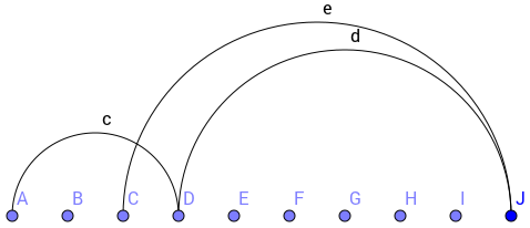
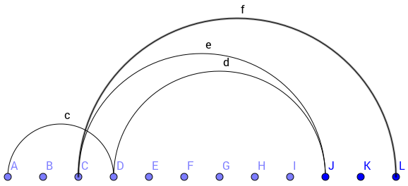
Figure 6: Non-trivial concatenation of loops $X=\{G_{4}^{(0)},G_{6}^{(3)},G_{8}^{(2)}\}^{10}$ and $X^{\prime}=\{G_{4}^{(0)},G_{6}^{(3)},G_{8}^{(2)},\underline{G_{10}^{(2)}}\}^{10}$ (only the largest arcs are shown)

(Here we assumed $\Delta_{{\tiny{[6,7,8,9,10,16,17,18,19,20,\dots,96,97,98,99,100]}}}=1$ to simplify the formula). Its configuration is drawn on the figure 6 (right).

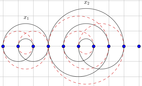
Figure 5: Concatenation of $x_{1},x_{2}\in S^{\prime}$ for $R=\Sigma_{0}$: compatible case

Now let’s extend the picture for $x_{3}$: The problem is that in this case $(m,n)=(16,16)$ the image is empty, so we should add some isolated points to the graph 6 (left).

Let

$$X=\{G_{i_{1}}^{(j_{1})},G_{i_{2}}^{(j_{2})},\dots,G_{i_{s}}^{(j_{s})}\}^{k}\in\mathcal{P}$$ (59)

be an element of path algebra of $Q_{\mathrm{univ}}(k)$, built as concatenation normal loops $G_{i_{1}},G_{i_{2}}$, each one shifted on the $j$-th position. For example, consider 3-union $\{G_{4}^{(0)},G_{6}^{(3)},G_{8}^{(2)}\}^{10}$. QR has unique solution; furthermore, we take $\Delta_{\tiny\yng(1,1,1)_{7}}=1$ (denominator) to homogenise the resulting formula. Here is the associated quiver:

$$Q(X)=\lx@xy@svg{\hbox{\raise 0.0pt\hbox{\kern 5.5pt\hbox{{\hbox{\kern-5.5pt\raise-53.0pt\hbox{\hbox{\kern 3.0pt\raise-3.22223pt\hbox{$\textstyle{0}$}}}}}{\hbox{\kern 47.5pt\raise-53.0pt\hbox{\hbox{\kern 3.0pt\raise-3.22223pt\hbox{$\textstyle{1}$}}}}}{\hbox{\kern 47.5pt\raise-146.0pt\hbox{\hbox{\kern 3.0pt\raise-3.22223pt\hbox{$\textstyle{2}$}}}}}{\hbox{\kern 47.5pt\raise 0.0pt\hbox{\hbox{\kern 3.0pt\raise-3.22223pt\hbox{$\textstyle{3}$}}}}}{\hbox{\kern 214.5pt\raise 0.0pt\hbox{\hbox{\kern 3.0pt\raise-3.22223pt\hbox{$\textstyle{4}$}}}}}{\hbox{\kern 214.5pt\raise-146.0pt\hbox{\hbox{\kern 3.0pt\raise-3.22223pt\hbox{$\textstyle{5}$}}}}}{\hbox{\kern 287.5pt\raise-53.0pt\hbox{\hbox{\kern 3.0pt\raise-3.22223pt\hbox{$\textstyle{6}$}}}}}{\hbox{\kern 141.5pt\raise 0.0pt\hbox{\hbox{\kern 3.0pt\raise-3.22223pt\hbox{$\textstyle{7}$}}}}}{\hbox{\kern 141.5pt\raise-53.0pt\hbox{\hbox{\kern 3.0pt\raise-3.22223pt\hbox{$\textstyle{8}$}}}}}{\hbox{\kern 141.5pt\raise-146.0pt\hbox{\hbox{\kern 3.0pt\raise-3.22223pt\hbox{$\textstyle{9}$}}}}}\ignorespaces\ignorespaces\ignorespaces\ignorespaces\ignorespaces\ignorespaces{}\ignorespaces\ignorespaces\ignorespaces{\hbox{\lx@xy@drawline@}}\ignorespaces{\hbox{\kern 3.54253pt\raise-59.22223pt\hbox{\hbox{\kern 0.0pt\raise 0.0pt\hbox{\lx@xy@tip{1}\lx@xy@tip{-1}}}}}}\ignorespaces\ignorespaces\ignorespaces{\hbox{\lx@xy@drawline@}}\ignorespaces{\hbox{\lx@xy@drawline@}}\ignorespaces\ignorespaces\ignorespaces\ignorespaces\ignorespaces\ignorespaces\ignorespaces{}\ignorespaces\ignorespaces\ignorespaces{\hbox{\lx@xy@drawline@}}\ignorespaces{\hbox{\kern 47.5pt\raise-5.5pt\hbox{\hbox{\kern 0.0pt\raise 0.0pt\hbox{\lx@xy@tip{1}\lx@xy@tip{-1}}}}}}\ignorespaces\ignorespaces\ignorespaces{\hbox{\lx@xy@drawline@}}\ignorespaces{\hbox{\lx@xy@drawline@}}\ignorespaces\ignorespaces\ignorespaces\ignorespaces\ignorespaces\ignorespaces\ignorespaces\ignorespaces{}\ignorespaces{\hbox{\lx@xy@droprule}}\ignorespaces{\hbox{\kern 53.0pt\raise-139.77779pt\hbox{\hbox{\kern 0.0pt\raise 0.0pt\hbox{\lx@xy@tip{1}\lx@xy@tip{-1}}}}}}\ignorespaces{\hbox{\lx@xy@droprule}}{\hbox{\lx@xy@droprule}}\ignorespaces\ignorespaces\ignorespaces\ignorespaces\ignorespaces\ignorespaces\ignorespaces\ignorespaces{}\ignorespaces{\hbox{\lx@xy@droprule}}\ignorespaces{\hbox{\kern 53.0pt\raise-46.77779pt\hbox{\hbox{\kern 0.0pt\raise 0.0pt\hbox{\lx@xy@tip{1}\lx@xy@tip{-1}}}}}}\ignorespaces{\hbox{\lx@xy@droprule}}{\hbox{\lx@xy@droprule}}\ignorespaces\ignorespaces\ignorespaces\ignorespaces\ignorespaces\ignorespaces\ignorespaces{}\ignorespaces\ignorespaces\ignorespaces{\hbox{\lx@xy@drawline@}}\ignorespaces{\hbox{\kern 58.50002pt\raise-140.55908pt\hbox{\hbox{\kern 0.0pt\raise 0.0pt\hbox{\lx@xy@tip{1}\lx@xy@tip{-1}}}}}}\ignorespaces\ignorespaces\ignorespaces{\hbox{\lx@xy@drawline@}}\ignorespaces{\hbox{\lx@xy@drawline@}}\ignorespaces\ignorespaces\ignorespaces\ignorespaces\ignorespaces\ignorespaces\ignorespaces\ignorespaces{}\ignorespaces{\hbox{\lx@xy@droprule}}\ignorespaces{\hbox{\kern 141.5pt\raise-146.0pt\hbox{\hbox{\kern 0.0pt\raise 0.0pt\hbox{\lx@xy@tip{1}\lx@xy@tip{-1}}}}}}\ignorespaces{\hbox{\lx@xy@droprule}}{\hbox{\lx@xy@droprule}}\ignorespaces\ignorespaces\ignorespaces\ignorespaces\ignorespaces\ignorespaces\ignorespaces\ignorespaces{}\ignorespaces{\hbox{\lx@xy@droprule}}\ignorespaces{\hbox{\kern 58.50002pt\raise 0.0pt\hbox{\hbox{\kern 0.0pt\raise 0.0pt\hbox{\lx@xy@tip{1}\lx@xy@tip{-1}}}}}}\ignorespaces{\hbox{\lx@xy@droprule}}{\hbox{\lx@xy@droprule}}\ignorespaces\ignorespaces\ignorespaces\ignorespaces\ignorespaces\ignorespaces\ignorespaces{}\ignorespaces\ignorespaces\ignorespaces{\hbox{\lx@xy@drawline@}}\ignorespaces{\hbox{\kern 141.5pt\raise-49.90625pt\hbox{\hbox{\kern 0.0pt\raise 0.0pt\hbox{\lx@xy@tip{1}\lx@xy@tip{-1}}}}}}\ignorespaces\ignorespaces\ignorespaces{\hbox{\lx@xy@drawline@}}\ignorespaces{\hbox{\lx@xy@drawline@}}\ignorespaces\ignorespaces\ignorespaces\ignorespaces\ignorespaces\ignorespaces\ignorespaces{}\ignorespaces\ignorespaces\ignorespaces{\hbox{\lx@xy@drawline@}}\ignorespaces{\hbox{\kern 225.50002pt\raise-3.98535pt\hbox{\hbox{\kern 0.0pt\raise 0.0pt\hbox{\lx@xy@tip{1}\lx@xy@tip{-1}}}}}}\ignorespaces\ignorespaces\ignorespaces{\hbox{\lx@xy@drawline@}}\ignorespaces{\hbox{\lx@xy@drawline@}}\ignorespaces\ignorespaces\ignorespaces\ignorespaces\ignorespaces\ignorespaces\ignorespaces\ignorespaces{}\ignorespaces{\hbox{\lx@xy@droprule}}\ignorespaces{\hbox{\kern 152.50002pt\raise 0.0pt\hbox{\hbox{\kern 0.0pt\raise 0.0pt\hbox{\lx@xy@tip{1}\lx@xy@tip{-1}}}}}}\ignorespaces{\hbox{\lx@xy@droprule}}{\hbox{\lx@xy@droprule}}\ignorespaces\ignorespaces\ignorespaces\ignorespaces\ignorespaces\ignorespaces\ignorespaces{}\ignorespaces\ignorespaces\ignorespaces{\hbox{\lx@xy@drawline@}}\ignorespaces{\hbox{\kern 214.5pt\raise-3.99072pt\hbox{\hbox{\kern 0.0pt\raise 0.0pt\hbox{\lx@xy@tip{1}\lx@xy@tip{-1}}}}}}\ignorespaces\ignorespaces\ignorespaces{\hbox{\lx@xy@drawline@}}\ignorespaces{\hbox{\lx@xy@drawline@}}\ignorespaces\ignorespaces\ignorespaces\ignorespaces\ignorespaces\ignorespaces\ignorespaces{}\ignorespaces\ignorespaces\ignorespaces{\hbox{\lx@xy@drawline@}}\ignorespaces{\hbox{\kern 288.11458pt\raise-59.22223pt\hbox{\hbox{\kern 0.0pt\raise 0.0pt\hbox{\lx@xy@tip{1}\lx@xy@tip{-1}}}}}}\ignorespaces\ignorespaces\ignorespaces{\hbox{\lx@xy@drawline@}}\ignorespaces{\hbox{\lx@xy@drawline@}}\ignorespaces\ignorespaces\ignorespaces\ignorespaces\ignorespaces\ignorespaces\ignorespaces{}\ignorespaces\ignorespaces\ignorespaces{\hbox{\lx@xy@drawline@}}\ignorespaces{\hbox{\kern 215.12067pt\raise-139.77779pt\hbox{\hbox{\kern 0.0pt\raise 0.0pt\hbox{\lx@xy@tip{1}\lx@xy@tip{-1}}}}}}\ignorespaces\ignorespaces\ignorespaces{\hbox{\lx@xy@drawline@}}\ignorespaces{\hbox{\lx@xy@drawline@}}\ignorespaces\ignorespaces\ignorespaces\ignorespaces\ignorespaces\ignorespaces\ignorespaces\ignorespaces{}\ignorespaces{\hbox{\lx@xy@droprule}}\ignorespaces{\hbox{\kern 214.5pt\raise-146.0pt\hbox{\hbox{\kern 0.0pt\raise 0.0pt\hbox{\lx@xy@tip{1}\lx@xy@tip{-1}}}}}}\ignorespaces{\hbox{\lx@xy@droprule}}{\hbox{\lx@xy@droprule}}\ignorespaces}}}} \textstyle{0} \textstyle{1} \textstyle{2} \textstyle{3} \textstyle{4} \textstyle{5} \textstyle{6} \textstyle{7} \textstyle{8} \textstyle{9} \textstyle{0} \textstyle{1} \textstyle{2} \textstyle{3} \textstyle{4} \textstyle{5} \textstyle{6} \textstyle{7} \textstyle{8} \textstyle{9}$$ (60)

Then $\tilde{P}_{\pm}(X)$ become homogeneous in $\Delta$:

$$\tilde{P}_{\pm}(X)= \left(s_{\tiny\yng(1,5)_{9}}+s_{\tiny\yng(1)_{0}}+s_{\tiny\yng(1,1)_{5}}+s_{\tiny\yng(1)_{1}}+s_{\tiny\yng(1)_{2}}+s_{\tiny\yng(1,1)_{4}}+s_{\tiny\yng(1)_{6}}+s_{\tiny\yng(1)_{3}}+s_{\tiny\yng(1,5)_{8}}+s_{\tiny\yng(1)_{7}}\right)\Delta_{\tiny\yng(1)_{6}}+$$ (61)

$$+\left(s_{\tiny\yng(1,1)_{0}}+s_{\tiny\yng(1,1,5)_{8}}+s_{\tiny\yng(1,1)_{3}}+s_{\tiny\yng(1,1)_{1}}+s_{\tiny\yng(1,1,1)_{6}}+s_{\tiny\yng(1,1,1)_{5}}+s_{\tiny\yng(1,1)_{2}}+s_{\tiny\yng(1,1,1)_{4}}+s_{\tiny\yng(1,1)_{7}}+s_{\tiny\yng(1,1,5)_{9}}\right)\Delta_{\tiny\yng(1,1,1)_{6}}+$$

$$+\left(s_{\tiny\yng(1,1,1)_{2}}+s_{\tiny\yng(1,1,1,1)_{7}}+s_{\tiny\yng(1,1,1,1)_{6}}+s_{\tiny\yng(1,1,1)_{3}}+s_{\tiny\yng(1,1,1,1)_{5}}+s_{\tiny\yng(1,1,1,1)_{4}}+s_{\tiny\yng(1,1,1,5)_{9}}+s_{\tiny\yng(1,1,1)_{0}}+s_{\tiny\yng(1,1,1)_{1}}+s_{\tiny\yng(1,1,1,1,5)_{8}}\right)\Delta_{\tiny\yng(1,1,1,1)_{6}}+$$

$$+\left(s_{\tiny\yng(1,1,1,1,5)_{9}}+s_{\tiny\yng(1,1,1,5)_{8}}+s_{\tiny\yng(1,1,1,1)_{1}}+s_{\tiny\yng(1,1,1,1,1)_{7}}+s_{\tiny\yng(1,1,1,1,1)_{5}}+s_{\tiny\yng(1,1,1,1,1)_{6}}+s_{\tiny\yng(1,1,1,1)_{0}}+s_{\tiny\yng(1,1,1,1)_{2}}+s_{\tiny\yng(1,1,1,1)_{3}}+s_{\tiny\yng(1,1,1,1,1)_{4}}\right)\Delta_{\tiny\yng(1,1,1,1,1)_{6}}+$$

$$+s_{\tiny\yng(1,1,1,1,1)_{0}}+s_{\tiny\yng(1,1,1,1,1)_{1}}+s_{\tiny\yng(5)_{8}}+s_{\tiny\yng(1)_{5}}+s_{\tiny\yng(1,1,1,1,1)_{3}}+s_{\tiny\yng(5)_{9}}+s_{\tiny\yng(1)_{4}}+s_{\tiny\yng(1,1)_{6}}+s_{\tiny\yng(1,1,1,1,1)_{2}}$$

Remark: we can see only antisymmetric coefficients $\Delta$ here! To extend this case for $G_{10}$ one should exclude $G_{8}^{(2)}$.

The resulting picture is that each loop can be scaled separately, such that increasing $k,s$ simultaneously does not change the consistency of QR. Our next aim is to investigate asymptotical properties, derived from $\{G_{i_{1}}^{(j_{1})},G_{i_{2}}^{(j_{2})},\dots,G_{i_{s}}^{(j_{s})}\}^{k}$ when $k,s\to\infty$. This is of further development.

References

- [1] Alistair Savage, Peter Tingley Quiver grassmannians, quiver varieties and the preprojective algebra // http://arxiv.org/abs/0909.3746
- [2] Maxim Kontsevich, Yan Soibelman Lectures on motivic Donaldson-Thomas invariants and wall-crossing formulas // arxiv preprint, 2011
- [3] Oliver Lorscheid, Thorsten Weist Quiver Grassmannians of type extended Dynkin type D - Part 1: Schubert systems and decompositions into affine spacess // https://arxiv.org/abs/1507.00392
- [4] Oliver Lorscheid, Thorsten Weist Homogeneous coordinates for quiver grassmannians // http://arxiv.org/abs/1607.01058v1
- [5] Oliver Lorscheid, Thorsten Weist Quiver Grassmannians of extended Dynkin type D - Part 2: Schubert decompositions and F-polynomials // http://arxiv.org/abs/1507.00395