1
Information-Theoretic Bounds and Approximations
in Neural Population Coding
Wentao Huang
whuang21@jhmi.edu
Department of Biomedical Engineering, Johns Hopkins University
School of Medicine, Baltimore, MD 21205, U.S.A., and Cognitive and Intelligent
Lab of China Electronics Technology Group Corporation, Beijing 100846, China.
Kechen Zhang
kzhang4@jhmi.edu
Department of Biomedical Engineering, Johns
Hopkins University School of Medicine, Baltimore, MD 21205, U.S.A.
Abstract
While Shannon’s mutual information has wide spread applications in many disciplines, for practical applications it is often difficult to calculate its value accurately for high-dimensional variables because of the curse of dimensionality. This paper is focused on effective approximation methods for evaluating mutual information in the context of neural population coding. For large but finite neural populations, we derive several information-theoretic asymptotic bounds and approximation formulas that remain valid in high-dimensional spaces. We prove that optimizing the population density distribution based on these approximation formulas is a convex optimization problem which allows efficient numerical solutions. Numerical simulation results confirmed that our asymptotic formulas were highly accurate for approximating mutual information for large neural populations. In special cases, the approximation formulas are exactly equal to the true mutual information. We also discuss techniques of variable transformation and dimensionality reduction to facilitate computation of the approximations.
1 Introduction
Shannon’s mutual information (MI) provides a quantitative characterization of the association between two random variables by measuring how much knowing one of the variables reduces uncertainty about the other (Shannon,, 1948). Information theory has become a useful tool for neuroscience research (Rieke et al.,, 1997; Borst & Theunissen,, 1999; Pouget et al.,, 2000; Laughlin & Sejnowski,, 2003; Brown et al.,, 2004; Quiroga & Panzeri,, 2009), with applications to various problems such as sensory coding problems in the visual systems (Eckhorn & Pöpel,, 1975; Optican & Richmond,, 1987; Atick & Redlich,, 1990; McClurkin et al.,, 1991; Atick et al.,, 1992; Becker & Hinton,, 1992; Van Hateren,, 1992; Gawne & Richmond,, 1993; Tovee et al.,, 1993; Bell & Sejnowski,, 1997; Lewis & Zhaoping,, 2006) and the auditory systems (Chechik et al.,, 2006; Gourévitch & Eggermont,, 2007; Chase & Young,, 2005).
One major problem encountered in practical applications of information theory is that the exact value of mutual information is often hard to compute in high-dimensional spaces. For example, suppose we want to calculate the mutual information between a random stimulus variable that requires many parameters to specify and the elicited noisy responses of a large population of neurons. In order to accurately evaluate the mutual information between the stimuli and the responses, one has to average over all possible stimulus patterns and over all possible response patterns of the whole population. This averaging quickly leads to a combinatorial explosion as either the stimulus dimension or the population size increases. This problem occurs not only when one computes MI numerically for a given theoretical model but also when one estimates MI empirically from experimental data.
Even when the input and output dimensions are not that high, MI estimate from experimental data tends to have a positive bias due to limited sample size (Miller,, 1955; Treves & Panzeri,, 1995). For example, a perfectly flat joint probability distribution implies zero MI, but an empirical joint distribution with fluctuations due to finite data size appears to suggest a positive MI. The error may get much worse as the input and output dimensions increase because a reliable estimate of MI may require exponentially more data points to fill the space of the joint distribution. Various asymptotic expansion methods have been proposed to reduce the bias in MI estimate (Miller,, 1955; Carlton,, 1969; Treves & Panzeri,, 1995; Victor,, 2000; Paninski,, 2003). Other estimators of MI have also been studied, such as those based on k-nearest neighbor (Kraskov et al.,, 2004) and minimal spanning trees (Khan et al.,, 2007). However, it is not easy for these methods to handle the general situation with high-dimensional inputs and high-dimensional outputs.
For numerical computation of MI for a given theoretical model, one useful approach is Monte Carlo sampling, a convergent method that may potentially reaches arbitrary accuracy (Yarrow et al.,, 2012). However, its stochastic and inefficient computational scheme makes it unsuitable for many applications. For instance, to optimize the distribution of a neural population for a given set of stimuli, one may want to slightly alter the population parameters and see how the perturbation affects the MI, but a tiny change of MI can be easily drowned out by the inherent noise in the Monte Carlo method.
An alternative approach is to use information-theoretic bounds and approximations to simplify calculations. For example, the Cramér-Rao lower bound (Rao,, 1945) tell us that the inverse of Fisher information (FI) is a lower bound to the mean square decoding error of any unbiased decoder. Fisher information is useful for many applications partly because it is often much easier to calculate than MI (see e.g., Zhang et al.,, 1998; Zhang & Sejnowski,, 1999; Abbott & Dayan,, 1999; Bethge et al.,, 2002; Harper & McAlpine,, 2004; Toyoizumi et al.,, 2006).
A link between MI and FI has been studied by several researchers (Clarke & Barron,, 1990; Rissanen,, 1996; Brunel & Nadal,, 1998; Sompolinsky et al.,, 2001). Clarke & Barron, (1990) first derived an asymptotic formula between the relative entropy and FI for parameter estimation from independent and identically distributed (i.i.d.) observations with suitable smoothness conditions. Rissanen, (1996) generalized it in the framework of stochastic complexity for model selection. Brunel & Nadal, (1998) presented an asymptotic relationship between the MI and FI in the limit of a large number of neurons. The method was extended to discrete inputs by Kang & Sompolinsky, (2001). More general discussions about this also appeared in other papers (e.g. Ganguli & Simoncelli,, 2014; Wei & Stocker,, 2015). However, for finite population size, the asymptotic formula may lead to large errors, especially for high-dimensional inputs as detailed in sections 2.2 and 4.1.
In this paper, our main goal is to improve FI approximations to MI for finite neural populations especially for high-dimensional inputs. Another goal is to discuss how to use these approximations to optimize neural population coding. We will present several information-theoretic bounds and approximation formulas and discuss the conditions under which they are established in section 2, with detailed proofs given in Appendix. We also discuss how our approximation formulas are related to other statistical estimators and information-theoretic bounds, such as Cramér-Rao bound and van Trees’ Bayesian Cramér-Rao bound (section 3). In order to better apply the approximation formulas in high-dimensional input space, we propose some useful techniques in section 4, including variable transformation and dimensionality reduction, which may greatly reduce the computational complexity for practical applications. Finally, in section 5, we discuss how to use the approximation formulas for the optimization of information transfer for neural population coding.
2 Bounds and Approximations for Mutual Information in Neural Population Coding
2.1 Mutual Information and Notations
Suppose the input is a -dimensional vector, , , , , the outputs of neurons are denoted by a vector, , , , . In this paper we denote random variables by upper case letters, e.g., random variables and , in contrast to their vector values and . The MI (denoted as below) between and is defined by (Cover & Thomas,, 2006)
| (2.1) |
where , , , , and the integration symbol is for the continuous variables and can be replaced by summation symbol for discrete variables. The probability density function (p.d.f.) of , , satisfies
| (2.2) |
The MI in (2.1) may also be expressed equivalently as
| (2.3) |
where is the entropy of random variable :
| (2.4) |
and denotes expectation:
| (2.5) | |||
| (2.6) | |||
| (2.7) |
Next, we introduce the following notations,
| (2.8) | |||
| (2.9) | |||
| (2.10) |
and
| (2.11) | ||||
| (2.12) |
where denotes the matrix determinant, and
| (2.13) | |||
| (2.14) | |||
| (2.15) |
Here is FI matrix, which is symmetric and positive-semidefinite, and ′ and ′′ denote the first and second derivative for , respectively; that is, and . If is twice differentiable for , then
| (2.16) |
We denote the Kullback-Leibler (KL) divergence as
| (2.17) |
and define
| (2.18) |
as the neighborhoods of , and its complementary set as
| (2.19) |
where is a positive number.
2.2 Information-Theoretic Asymptotic Bounds and Approximations
In large limit, Brunel & Nadal, (1998) proposed an asymptotic relationship between MI and FI and gave a proof in the case of one-dimensional input. Another proof is given by Sompolinsky et al., (2001) although there appears to be an error in their proof when replica trick is used (see Eq. (B1) in their paper; their Eq. (B5) does not follow directly from the replica trick). For large but finite , is usually a good approximation as long as the inputs are low-dimensional. For the high-dimensional inputs, the approximation may no longer be valid. For example, suppose is a normal distribution with mean and covariance matrix and is a normal distribution with mean and covariance matrix ,
| (2.20) |
where is a deterministic matrix and is the identity matrix. The MI is given by (see Verdu,, 1986; Guo et al.,, 2005, for details)
| (2.21) |
If , then . Notice that here . When and , then by (2.21) and matrix determinant lemma, we have
| (2.22) |
and by (2.11),
| (2.23) |
which is obviously incorrect as an approximation to . For high-dimensional inputs, the determinant may become close to zero in practical applications. When the FI matrix becomes degenerate, the regularity condition ensuring the Cramér-Rao paradigm of statistics is violated (Amari & Nakahara,, 2005), in which case using as a proxy for incurs large errors.
In the following, we will show is a better approximation of for high-dimensional inputs. For instance, for the above example, we can verify that
| (2.24) |
which is exactly equal to the MI given in (2.21).
2.2.1 Regularity Conditions
First, we consider the following regularity conditions for and :
C1: and are twice continuously differentiable for almost every , where is a convex set; is positive definite and , where denotes the Frobenius norm of a matrix; the following conditions hold
| (2.25a) | |||
| (2.25b) | |||
| (2.25c) | |||
| (2.25d) | |||
| and there exists an for such that | |||
| (2.25e) | |||
| where indicates the big-O notation. | |||
C2: The following condition is satisfied:
| (2.26a) | |||
| for , and there exists such that | |||
| (2.26b) | |||
| for all , and with , where denotes the probability of given . | |||
The regularity conditions C1 and C2 are needed to prove theorems in later sections. They are expressed in mathematical forms that are convenient for our proofs although their meanings may seem opaque at the first glance. In the following, we will examine these conditions more closely. We will use specific examples to make interpretations of these conditions more transparent.
Remark 2.1.
In this paper we assume that the probability distributions and are piecewise twice continuously differentiable. This is because we need to use Fisher information to approximate mutual information, and Fisher information requires derivatives that make sense only for continuous variables. Therefore, the methods developed in this paper apply only to continuous input variables or stimulus variables. For discrete input variables, we need alternative methods for approximating MI and we will address this issue in a separate publication.
Conditions (2.25a) and (2.25b) state that the first and the second derivatives of have finite values for any given . These two conditions are easily satisfied by commonly encountered probability distributions because they only require finite derivatives within , the set of allowable inputs, and derivatives do not need to be finitely bounded.
Remark 2.2.
Conditions (2.25c)–(2.26a) constrain how the first and the second derivatives of scale with , the number of neurons. These conditions are easily met when is conditionally independent or when the noises of different neurons are independent, i.e., .
We emphasize that it is possible to satisfy these conditions even when is not independent or when the noises are correlated, as shown later. Here we first examine these conditions closely assuming independence. For simplicity, our demonstration below is based on a one-dimensional input variable (). The conclusions are readily generalizable to higher dimensional inputs () because is fixed and does not affect the scaling with .
Assuming independence, we have with , and the left-hand side of (2.25c) becomes
| (2.27) |
where the final result contains only two terms with even numbers of duplicated indices while all other terms in the expansion vanish because any unmatched or lone index (from ) should yield a vanishing average:
| (2.28) |
Thus, condition (2.25c) is satisfied as long as and are bounded by some finite numbers, say, and , respectively, because now (2.27) should scale as . For instance, a Gaussian distribution always meets this requirement because the averages of the second and fourth powers are proportional to the second and fourth moments, which are both finite. Note that the argument above works even if is not finitely bounded but scales as .
Similarly, under the assumption of independence, the left-hand side of (2.25d) becomes
| (2.29) |
where in the second step, the only remaining terms are the squares while all other terms in the expansion with have vanished because . Thus, condition (2.25d) is satisfied as long as and are bounded so that (2.29) scales as .
Condition (2.25e) is easily satisfied under the assumption of independence. It is easy to show that this condition holds when is bounded.
Condition (2.26a) can be examined using similar arguments used for (2.27) and (2.29). Assuming independence, we rewrite the left-hand side of (2.26a) as:
| (2.30) |
where is an even number. Any term in the expansion with an unmatched index should vanish, as in the cases of (2.27) and (2.29). When and are bounded, the leading term with respect to scaling with is the product of squares as shown at the end of (2.30) because all the other non-vanishing terms increase more slowly with . Thus (2.30) should scale as , which trivially satisfies condition (2.26a).
Remark 2.3.
For neurons with correlated noises, if there exists an invertible transformation that maps to such that becomes conditionally independent, then conditions C1 and C2 are easily met in the space of the new variables by the discussion in Remark 2.2. This situation is best illustrated by the familiar example of a population of neurons with correlated noises that obey a multivariate Gaussian distribution:
| (2.31) |
where is an invertible covariance matrix and describes the mean responses with being the parameter vector. Using the following transformation,
| (2.32) | ||||
| (2.33) |
we obtain the independent distribution:
| (2.34) |
In the special case when the correlation coefficient between any pair of neurons is a constant , , the noise covariance can be written as
| (2.35) |
where is a constant, is the identity matrix, . The desired transformation in (2.32) and (2.33) is given explicitly by
| (2.36) |
where
| (2.37) |
The new response variables defined in (2.32) and (2.33) now read:
| (2.38) | ||||
| (2.39) |
Now we have the derivatives:
| (2.40) | |||
| (2.41) |
where and are finite as long as and are finite. Conditions C1 and C2 are satisfied when the derivatives and their powers are finitely bounded as shown before.
The example above shows explicitly that it is possible to meet conditions C1 and C2 even when the noises of different neurons are correlated. More generally, if a nonlinear transformation exists that maps correlated random variables into independent variables, then by similar argument, conditions C1 and C2 are satisfied when the derivatives of the log likelihood functions and their powers in the new variables are finitely bounded. Even when the desired transformation does not exist or is unknown, it does not necessarily imply that conditions C1 and C2 must be violated.
While the exact mathematical conditions for the existence of the desired transformation are unclear, let us consider a specific example. If a joint probability density function can be morphed smoothly and reversibly into a flat or constant density in a cube (hypercube), which is a special case of an independent distribution, then this morphing is the desired transformation. Here we may replace the flat distribution by any known independent distribution and the argument above should still work. So the desired transformation may exist under rather general conditions.
For correlated random variables, one may use algorithms such as independent component analysis to find an invertible linear mapping that makes the new random variables as independent as possible (Bell & Sejnowski,, 1997), or use neural networks to find related nonlinear mappings (Huang & Zhang,, 2017). These methods do not directly apply to the problem of testing conditions C1 and C2 because they work for a given network size and further development is needed to address the scaling behavior in the large network limit .
Finally, we note that the value of the MI of the transformed independent variables is the same as the MI of the original correlated variables because of the invariance of MI under invertible transformation of marginal variables. A related discussion is in Theorem 4.1 which involves a transformation of the input variables rather than a transformation of the output variables as needed here.
Remark 2.4.
Condition (2.26b) is satisfied if a positive number and a positive integer exist such that
| (2.42) |
for all , where
| (2.43) |
and means that the matrix is negative definite. A proof is as follows.
First note that in (2.43) if or , then . Following Markov’s inequality, condition C2 and (A.19) in the Appendix, for the complementary set of , , we have
| (2.44) |
where
| (2.45) |
Define the set,
| (2.46) |
then it follows from the Markov’s inequality and (2.42) that
| (2.47) |
Hence, we get
which yields the condition (2.26b).
2.2.2 Asymptotic Bounds and Approximations for Mutual Information
Let
| (2.51) |
and it follows from conditions C1 and C2 that
| (2.52) |
Moreover, if is conditionally independent, then by an argument similar to the discussion in Remark 2.2, we can verify that the condition is easily met.
In the following we state several conclusions about the MI, and their proofs are given in Appendix.
Lemma 2.1.
Lemma 2.2.
If conditions C1 and C2 hold, , then the MI has an asymptotic lower bound for integer ,
| (2.56) |
Moreover, if condition C1 holds but Eqs. (2.25c) and (2.25d) are replaced by (2.54a) and (2.54b), and inequality (2.26b) in C2 also holds for , then the MI has the following asymptotic lower bound for integer ,
| (2.57) |
Theorem 2.1.
If conditions C1 and C2 hold, , then the MI has the following asymptotic equality for integer ,
| (2.58) |
For more relaxed conditions, suppose condition C1 holds but Eqs. (2.25c) and (2.25d) are replaced by (2.54a) and (2.54b), and inequality (2.26b) in C2 also holds for , then the MI has an asymptotic equality for integer ,
| (2.59) |
Theorem 2.2.
Suppose and are symmetric and positive-definite. Let
| (2.60) | |||
| (2.61) |
then
| (2.62) |
where indicating matrix trace; moreover, if is positive-semidefinite, then
| (2.63) |
On the other hand, if
| (2.64) |
for some , then
| (2.65) |
Remark 2.5.
In general, we only need to assume that and are piecewise twice continuously differentiable for . In this case, Lemma 2.1, Lemma 2.2 and Theorem 2.1 can still be established. For more general cases, such as discrete or continuous inputs, we have also derived a general approximation formula for MI from which we can easily derive formula for and which will be discussed in separate paper.
2.3 Approximations of Mutual Information in Neural Populations with Finite Size
In the preceding section we have provided several bounds, including both lower and upper bounds, and asymptotic relationships for the true MI in the large (network size) limit. In the following, we will discuss effective approximations to the true MI in the case of finite . Here we only consider the case of continuous inputs and will discuss the case of discrete inputs in another paper.
Theorem 2.1 tells us that under suitable conditions, we can use to approximate for a large but finite (e.g. ); that is
| (2.66) |
Moreover, by Theorem 2.2, we know that if with positive-semidefinite or holds (see Eqs. 2.60 and 2.64), then by (2.63), (2.65) and (2.66) we have
| (2.67) |
Define
| (2.68) | |||
| (2.69) |
where is positive-definite, is a symmetric matrix depending on and . Suppose , if we replace by in Theorem 2.1, then we can prove equations (2.58) and (2.59) in a manner similar to the proof of Theorem 2.1. Considering a special case where , (e.g. ) and , then we can no longer use the asymptotic formulas in Theorem 2.1. However, if we substitute for by choosing an appropriate such that is positive-definite and , then we can use (2.58) or (2.59) as the asymptotic formulas.
If we assume and are positive-definite and
| (2.70) |
then similar to the proof of Theorem 2.2, we have
| (2.71) |
and
For large , we usually have .
It is more convenient to redefine the following quantities:
| (2.72) | |||
| (2.73) | |||
| (2.74) |
and
| (2.75) |
Notice that if is twice differentiable for and
| (2.76) |
then
| (2.77) |
For example, if is a normal distribution, , then
| (2.78) |
Similar to the proof of Theorem 2.2, we can prove that
| (2.79) |
where
| (2.80) |
We find that is often a good approximation of MI even for relatively small . However, we cannot guarantee that is always positive-semidefinite in Eqs. (2.14), and as a consequence, it may happen that is very small for small , is not positive-definite and is not a real number. In this case, is not a good approximation to but is still a good approximation. Generally, if is always positive-semidefinite, then or is a better approximation than , especially when be close to a normal distribution.
In the following we will give an example of 1-D inputs. High-dimensional inputs will be discussed in section 4.1.
2.3.1 A Numerical Comparison for 1-D Stimuli
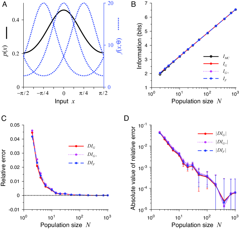
Considering the Poisson neuron model (see Eq. 5.7 in section 5.1 for details), the tuning curve of the n-th neuron, , takes the form of circular normal or von Mises distribution
| (2.81) |
where , , , with , , and , and the centers , , , of the neurons are uniformly distributed on interval , i.e., , with and . Suppose the distribution of -D continuous input () has the form
| (2.82) |
where is a constant set to , and is the normalization constant. Figure 1A shows graphs of the input distribution and the tuning curves with different centers , , .
To evaluate the precision of the approximation formulas, we use Monte Carlo (MC) simulation to approximate MI . For MC simulation, we first sample an input by the distribution , then generate the neural response by the conditional distribution , where , , , . The value of MI by MC simulation is calculated by
| (2.83) |
where is given by
| (2.84) |
and for .
To evaluate the accuracy of MC simulation, we compute the standard deviation
| (2.85) |
where
| (2.86) | ||||
| (2.87) |
and is the -th entry of the matrix with samples taken randomly from the integer set , , , by a uniform distribution. Here we set , and .
For different ,,,,,,,,,,,,,, we compare with , and , which are illustrated in Figure 1B–D. Here we define the relative error of approximation, e.g., for , as
| (2.88) |
and the relative standard deviation
| (2.89) |
Figure 1B shows how the values of , , and change with neuron number , and Figure 1C and 1D show their relative errors and the absolute values of the relative errors with respect to . From Figure 1B–D we can see that the values of , and are all very close to one another and the absolute values of their relative errors are all very small. The absolute values are less than when and less than when . However, for the high-dimensional inputs, there will be a big difference between , and in many cases (see section 4.1 for more details).
3 Statistical Estimators and Neural Population Decoding
Given the neural response elicited by the input , we may infer or estimate the input from the response. This procedure is sometimes referred to as decoding from the response. We need to choose an efficient estimator, or a function that maps the response to an estimate of the true stimulus . The Maximum Likelihood (ML) estimator defined by
| (3.1) |
is known to be efficient in large limit. According to the Cramér-Rao lower bound (Rao,, 1945), we have the following relationship between the covariance matrix of any unbiased estimator, , and the FI matrix ,
| (3.2) |
where is an unbiased estimation of from the response , and means that matrix is positive-semidefinite. Thus
| (3.3) |
On the other hand, the MI between and is given by
| (3.4) |
where is the entropy of random variable and is its conditional entropy of random variable given . Since the maximum entropy probability distribution is Gaussian, satisfies
| (3.5) |
Therefore, from (3.4) and (3.5), we get
| (3.6) |
The data processing inequality (Cover & Thomas,, 2006) states that post-processing cannot increase information, so that we have
| (3.7) |
Here we can not directly obtain as in Brunel & Nadal, (1998) when and . The simulation results in Figure 1 also show that is not a lower bound of .
For biased estimators, the van Trees’ Bayesian Cramér-Rao bound (Van Trees & Bell,, 2007) provides a lower bound:
| (3.8) |
It follows from (2.75), (3.6) and (3.8) that
| (3.9) | ||||
| (3.10) | ||||
| (3.11) |
We may also regard decoding as Bayesian inference. By Bayes’ rule,
| (3.12) |
According to the Bayesian decision theory, if we know the response , from the prior and the likelihood , we can infer an estimation of the true stimulus , , for example,
| (3.13) |
which is also called Maximum A Posteriori (MAP) estimation.
Consider a loss function for estimation,
| (3.14) |
which is minimized when reaches its maximum. Now the conditional risk is
| (3.15) |
and the overall risk is
| (3.16) |
Then it follows from (2.3) and (3.16) that
| (3.17) |
Comparing (2.12), (2.66) and (3.17), we find
| (3.18) |
Hence, maximizing MI (or ) means minimizing the overall risk for a determinate . Therefore, we can get the optimal Bayesian inference via optimizing MI (or ).
By the Cramér-Rao lower bound, we know that the inverse of FI matrix reflects the accuracy of decoding (see Eq. 3.2). provides some knowledge about the prior distribution ; for example, is the covariance matrix of input when is a normal distribution. is small for a flat prior (poor prior) and large for a sharp prior (good prior). Hence, if the prior is flat or poor and the knowledge about model is rich, then the MI is governed by the knowledge of model, which results in a small (Eq. 2.64) and . Otherwise, the prior knowledge has a great influence on MI , which results in a large and .
4 Variable Transformation and Dimensionality Reduction in Neural Population Coding
For low-dimensional input and large , both are are good approximations of MI , but for high-dimensional input , a large value of may lead to a large error of , in which case (or ) is a better approximation. It is difficult to directly apply the approximation formula when we do not have an explicit expression of or . For many applications, we do not need to know the exact value of and only care about the value of (see section 5). From (2.12), (2.22) and (2.78), we know that if is close to a normal distribution, we can easily approximate and ot obtain and . When is not a normal distribution, we can employ a technique of variable transformation to make it closer to a normal distribution, as discussed below.
4.1 Variable Transformation
Suppose is an invertible and differentiable mapping:
| (4.1) |
and . Let denotes the p.d.f. of random variable and
| (4.2) |
Then we have the following conclusions, the proofs of which are given in Appendix.
Theorem 4.1.
The MI is equivariant under the invertible transformations. More specifically, for the above invertible transformation , the MI in (2.1) is equal to
| (4.3) |
Furthermore, suppose and fulfill the conditions C1, C2 and , then we have
| (4.4) | ||||
| (4.5) |
where is the entropy of random variable and satisfies
| (4.6) |
and denotes the Jacobian matrix of ,
| (4.7) |
Corollary 4.1.
Suppose is a normal distribution,
| (4.8) |
where , for , , , , is a deterministic matrix, is a deterministic invertible matrix and is an invertible and differentiable function. If has also a normal distribution, , then
| (4.9) |
where
| (4.10) | |||
| (4.11) | |||
| (4.12) |
Remark 4.1.
Consider the eigendecompositons of and as given by
| (4.13) | |||
| (4.14) |
where and are orthogonal matrices; and are eigenvalue matrices, and . Then by (2.11) and (4.9) we have
| (4.15) | ||||
| (4.16) |
and
| (4.17) |
Now consider two special cases. If , then by (4.17) we get
| (4.18) |
If , then
| (4.19) |
Here , . The FI matrix and become degenerate when and .
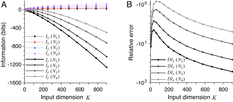
From (4.18) and (4.19) we see that if either or becomes degenerate, then . This may happen for high-dimensional stimuli. For a specific example, consider a random matrix defined as follows. Here we first generate elements , (, , , ; , , , ) from a normal distribution . Then each column of matrix is normalized by . We randomly sample (set to ) image patches with size from Olshausen’s nature image dataset (Olshausen & Field,, 1996) as the inputs. Each input image patch was centered by subtracting its mean, i.e., , then let for , , , . Define matrix , , , and compute eigendecomposition
| (4.20) |
where is a orthogonal matrix and is a eigenvalue matrix with . Define
| (4.21) |
then
| (4.22) |
The distribution of random variable can be approximated by a normal distribution (see section 4.3 for more details). When , we have
| (4.23) | ||||
| (4.24) | ||||
| (4.25) |
The error of approximation is given by
| (4.26) |
and the relative error for is
| (4.27) |
Figure 2A shows how the values of and vary with the input dimension and the number of neurons (with , , , , and , , , ). The relative error is shown in Figure 2B. The absolute value of the relative error tends to decrease with but may grow quite large as increases. In Figure 2B, the largest absolute value of relative error is greater than , which occurs when and . Even the smallest is still greater than , which occurs when and . In this example, is a bad approximation of MI whereas and are strictly equal to the true MI across all parameters.
4.2 Dimensionality Reduction for Asymptotic Approximations
Suppose is partitioned into two sets of components, , with
| (4.28) | ||||
| (4.29) |
where , , , , and . Then, by Fubini’s theorem, the MI in (2.1) can be written as
| (4.30) |
where , and , .
First define
| (4.31c) | |||
| (4.31d) | |||
| where , and | |||
| (4.32a) | |||
| (4.32b) | |||
| Then we have the following results and their proofs are given in Appendix. | |||
Theorem 4.2.
Suppose matrices , and are positive-definite. If the matrix satisfies
| (4.33) |
with
| (4.34) |
then we have
| (4.35) |
with strict equality if and only if
| (4.36) |
where
| (4.37) |
Theorem 4.3.
Suppose matrices , and are positive-definite. If the matrix is positive-semidefinite and satisfies
| (4.38) |
with
| (4.39) | |||
| (4.40) |
then we have
| (4.41) |
with strict equality if and only if
| (4.42) |
where
| (4.43) |
Corollary 4.2.
If the random variables and are independent so that , is a normal distribution, and , , and are all positive-definite and satisfy (4.38), then we have
| (4.44) | ||||
| (4.45) |
with strict equality if and only if
| (4.46) |
where
| (4.47a) | |||
| (4.47b) | |||
| (4.47c) | |||
Remark 4.2.
Sometimes we are concerned only with calculating the determinant of matrix with a given . Theorem 4.2 and Theorem 4.3 provide a dimensionality reduction method for computing or , by which we only need to compute and separately. To apply the approximation (4.35), we do not need to strictly require ; instead we only need to require
| (4.48) |
Similarly, the inequality can be substituted by
| (4.49) |
By (4.44) and the second mean value theorem for integrals, we get
| (4.50) |
for some fixed . When is small, should be close to the mean: . It follows from Theorem 2.1 and Corollary 4.2 that the approximate relationship holds. However, Eq. (4.50) implies that is determined only by the first component . Hence, there is little impact on information transfer by the minor component (i.e. ) for the high-dimensional input . In other words, the information transfer is mainly determined by the first component and we can omit the minor component .
4.3 Further Discussion
Suppose is a zero-mean vector, and if it is not, then let The covariance matrix of is given by
| (4.51) |
where is a orthogonal matrix whose k-th column is the eigenvector of x, and is diagonal matrix whose diagonal elements are the corresponding eigenvalues, i.e., with . With the whitening transformation,
| (4.52) |
the covariance matrix of becomes an identity matrix:
| (4.53) |
By the central limit theorem, the distribution of random variable should be closer to a normal distribution than the distribution of the original random variable ; that is, . Using Laplace’s method asymptotic expansion (MacKay,, 2003), we get
| (4.54) | ||||
| (4.55) |
In principal component analysis (PCA), the dataset is modeled by a multivariate gaussian. By a PCA-like whitening transformation (4.52) we can use the approximation (4.55) with Laplace’s method, which only requires that the peak be close to the mean and the random variable does not need to be an exact Gaussian distribution.
Given a orthogonal matrix , we define
| (4.62) |
Then it follows from (4.56)–(4.62) that
| (4.63) |
where
| (4.64) | ||||
| (4.65) | ||||
| (4.66) |
Suppose is partitioned into two sets of components, , and
| (4.67) | ||||
| (4.68) |
where , , and . Let
| (4.69) |
where
| (4.70) |
5 Optimization of Information Transfer in Neural Population Coding
5.1 Population Density Distribution of Parameters in Neural Populations
If is conditional independent, we can write
| (5.1) |
where denotes a -dimensional vector for parameters of the n-th neuron, and ; is the conditional p.d.f. of the output given . With the definition in (2.13), we have following proposition.
Proposition 5.1.
If is conditional independent as in Eq. (5.1), we have
| (5.2) |
where
| (5.3) |
, , and is the population density function of parameter vector :
| (5.4) |
with being the Dirac delta function.
Proof.
| (5.5) |
Remark 5.1.
Proposition 5.1 shows that can be regarded as a function of the population density of parameters, . If the p.d.f. of the input is given, we can find an appropriate to maximize MI .
For neuron model with Poisson spikes, we have
| (5.6) | |||
| (5.7) |
where ; is the tuning curve of the n-th neuron, , , , . Now we have
| (5.8) | ||||
| (5.9) |
Similarly, for neuron response model with Gaussian noise, we have
| (5.10) | |||
| (5.11) |
where is a constant standard deviation. Now we get
| (5.12) |
5.2 Optimal Population Distribution for Neural Population Coding
Suppose and fulfill conditions C1 and C2 and Eq. (5.1). Following the discussion of section 2.2, we define the following objective for maximizing MI ,
| (5.13) |
or equivalently,
| (5.14) |
where
| (5.15) | |||
| (5.16) | |||
| (5.17) |
Here is given in (2.15) and it generally can be substituted by (see Eq. 2.78).
When (see Eq. 2.64), the object function (5.13) can be reduced to
| (5.18) |
or equivalently,
| (5.19) |
The constraint condition for is given by
| (5.20) |
However, without further constraints on the neural populations, especially a limit on the peak firing rate, the capacity of the system may grow indefinitely, i.e. ; . The most common limitation on neural populations is the energy or power constraint. For neuron models with Poisson noise or Gaussian noise, a useful constraint is a limitation on the peak power,
| (5.21) |
where is the peak power. Under this constraint, maximizing or for independent neurons will result in for , , , .
Another constraint is a limitation on average power. For Poisson neurons given in Eq. (5.7),
| (5.22) |
which can also be written as
| (5.23) |
and for Gaussian noise neurons given in Eq. (5.11),
| (5.24) |
where is the maximum average energy cost.
In Eq. (5.15), we can approximate the continuous integral by a discrete summation for numerical computation,
| (5.25) |
where the positive integer denotes the number of subclasses in the neural population, and
| (5.26) |
If we do not know the specific form of but have samples, , , , , which are i.i.d. samples drawn from the distribution , then we can approximate the integral in (5.13) by the sample average:
| (5.27) |
Optimizing the objective (5.13) or (5.18) is a convex optimization problem (see Appendix for a proof).
Proposition 5.2.
The functions and are concave about .
Remark 5.2.
5.3 Necessary and Sufficient Conditions for Optimal Population Distribution
Applying the method of Lagrange multipliers for the optimization problem (5.13) and (5.20) yields
| (5.28) |
where is a constant and is a function of . According to Karush-Kuhn-Tucker (KKT) conditions (Boyd & Vandenberghe,, 2004), we have
| (5.29) |
and the necessary condition for optimal population density,
| (5.30) |
It follows from (5.29) and (5.30) that
| (5.31) | ||||
| (5.32) |
Since is a concave function of , Eq. (5.31) and (5.32) are the necessary and sufficient conditions for the optimization problem (5.13) and (5.20).
5.4 Channel Capacity for Neural Population Coding
If is unknown, then by Jensen’s inequality, we have
| (5.33) |
and the equality holds if and only if is a constant. Thus
| (5.34) | |||
| (5.35) |
assuming .
Let us consider a specific example. Suppose is a constant matrix, then it follows from (2.12) that
| (5.36) |
According to the maximum entropy probability distribution, we know that maximizing results in a uniformly distributed . Hence we have and coincides with the uniform distribution (see 5.35). In this case, the maximum can be regarded as the channel capacity for this neural population.
If we consider a constraint on random variables and assume that the covariance matrix of is and satisfies
| (5.37) |
then it follows from the maximum entropy probability distribution that
| (5.38) |
and the equality holds if and only if the p.d.f. of the input is a normal distribution: . Hence
| (5.39) |
where is the channel capacity of neural population. Here the equality holds if and only if , which is consistent with Eq. (5.37).
Furthermore, if (see 2.64), we have
| (5.40) |
Similarly, we also get
| (5.41) | |||
| (5.42) |
assuming . Here is the channel capacity of the neural population. The distribution coincides with the Jeffrey’s prior in Bayesian probability (Jeffreys,, 1961). In this case, if we suppose the covariance matrix of is , then similar to (5.38) and (5.39), we can get the channel capacity
| (5.43) |
with .
For another example, consider the Poisson neuron model given in (5.7) and suppose the input is one dimension, . It follows from (5.8) and (5.42) that
| (5.44) |
If , Eq. (5.44) becomes
| (5.45) |
Atick & Redlich, (1990) presented a redundancy measure to approximate Barlow’s optimality principle:
| (5.46) |
where is the channel capacity. Here for neural population coding we have and (or and . Hence we can minimize by choosing an appropriate to maximize (or ) and simultaneously satisfying (5.35) (or 5.42) (see Huang & Zhang,, 2017, for further details).
6 Discussion
In this paper we have derived several information-theoretic bounds and approximations for effective approximation of MI in the context of neural population coding for large but finite population size. We have found some regularity conditions under which the asymptotic bounds and approximations hold. Generally speaking, these regularity conditions are easy to meet. Special examples that satisfy these conditions include the cases when the likelihood function for the neural population responses is conditionally independent or has correlated noises with a multivariate Gaussian distribution. Under the general regularity conditions we have derived several asymptotic bounds and approximations of MI for a neural population and found some relationships among different approximations.
How to choose among these different asymptotic approximations of MI in a neural population with finite size ? For a flat prior distribution , we have ; that is, the two approximations and are about equally valid. For a sharply peaked prior distribution , is generally a better approximation to MI than . Under suitable conditions (e.g. C1 and C2) for low-dimensional inputs, , and are good approximations of MI not only for large but also for small . For high-dimensional inputs, the FI matrix (see Eq. 2.11) or matrix (see Eq. 2.15) often becomes degenerate, which causes a large error between and MI . Hence, in this situation, is a better approximation to MI than . For more convenient computation of the approximation, we have also introduced the approximation formula which may substitute for as a proxy of MI . For some special cases (see Corollary 4.1), and are strictly equal to the true MI . Our simulation results for the one-dimensional case shows that the approximations , , and are all highly precise compared with the true MI , even for small (Figure 1).
These approximation formulas satisfy additional constraints. By the Cramér-Rao lower bound, we know that is related to the covariance matrix of an unbiased estimator (see Eq. 3.3). By the van Trees’ Bayesian Cramér-Rao bound, we get a link between and the covariance matrix of a biased estimator (see Eq. 3.9). From the point of view of neural population decoding and Bayesian inference, there is a connection between MI (or ) and MAP (see Eq. 3.17).
For more efficient calculation of the approximation (or ) for high-dimensional inputs, we propose to apply an invertible transformation on the input variable so as to make the new variable closer to a normal distribution (see section 4.1). Another useful technique is dimensionality reduction which effectively approximates MI by further reducing the computational complexity for high-dimensional inputs. We found that could lead to huge errors as a proxy of the true MI for high-dimensional inputs even when and are strictly equal to the true MI .
These approximation formulas are potentially useful for optimization problems of information transfer in neural population coding. We have proven that optimizing the population density distribution of parameters is a convex optimization problem and have found a set of necessary and sufficient conditions. The approximation formulas are also useful for discussion of the channel capacity of neural population coding (section 5.4).
The information theory is a powerful tool for neuroscience and other disciplines, including diverse fields such as physics, information and communication technology, machine learning, computer vision, and bioinformatics. Finding effective approximation methods for computing MI is a key for many practical applications of information theory. Generally speaking, the FI matrix is easier to evaluate or approximate than MI. This is because calculation of MI involves averaging over both the input variable and the output variable (see Eq. 2.1), and typically also needs to be calculated from by another average over (see Eq. 2.2). By contrast, the FI matrix involves averaging over only (see Eq. 2.13). Furthermore, it is often easier to find analytical forms of FI for specific models such as a population of tuning curves with Poisson spike statistics. Taking into account the computational efficiency, for practical applications we suggest using or as a proxy of the true MI for most cases. These approximations could be very useful even when we do not need to know the exact value of MI. For example, for some optimization and learning problems, we only need to know how MI is affected by the conditional p.d.f. or likelihood function . In such situations, we may easily solve for the optimal parameters using the approximation formulas (Huang & Zhang,, 2017; Huang et al.,, 2017). Further discussions of the applications will be given in separate publications.
Acknowledgments
This work was supported partially by an NIH grant R01 DC013698.
Appendix: The Proofs
We consider a Taylor expanding of around . If is twice differentiable for , then by condition C1 we get
| (A.1) |
where
| (A.2) |
| (A.3) |
| (A.4) |
| (A.5) |
and
| (A.6) |
By condition C1, we know that the matrix is continuous and symmetric for and . By the definition of continuous functions, we can prove the following: for any , there is an such that for all
| (A.7) |
where
| (A.8) |
Hence,
| (A.9) |
Here , is a function of , , and
| (A.10) |
We define the sets
| (A.11) |
where
| (A.12) |
denotes an indicator random variable,
| (A.13) |
and
| (A.14) |
For all , we have , then
| (A.15) |
It follows from (A.3) and (A.6) that
| (A.16) |
and
| (A.17) |
and it follows from condition C1 that
| (A.18) |
Combining conditions C1 and C2, (A.3), (A.4) and (A.6), we find
| (A.19) |
together with the power mean inequality,
| (A.20) |
where , . Notice that . Here we note that for all conformable matrices and ,
| (A.21) |
A.1 Proof of Lemma 2.1
It follows from (A.1) that
| (A.24) |
For , according to the definitions in (A.13) and (A.14), we have
| (A.25) |
Then by condition C1, we get
| (A.26) |
where is a positive constant and . By (A.9), (A.17) and (A.24), we get
| (A.27) |
where , the last step in (A.27) follows from Jensen’s inequality, and
| (A.28) |
Integrating by parts yields
| (A.29) |
and
| (A.30) |
for some .
Then from (A.27), we get
| (A.31) |
where
| (A.32) |
Here notice that
| (A.33) |
and
| (A.34) |
Hence, from the consideration above, we find
| (A.35) |
A.2 Proof of Lemma 2.2
Define the sets
| (A.39) |
and
| (A.40) |
where , assuming and .
Consider the following equality,
| (A.43) |
For the last term in (A.43), Jensen’s inequality implies that
| (A.44) |
For the first term in (A.43), it follows from (A.40) and (A.9) that
| (A.45) |
The last term (A.45) is upper-bounded by
| (A.46) | |||
| (A.47) |
The term (A.46) is equal to
| (A.48) |
The term (A.47) is equal to
| (A.49a) | |||
| (A.49b) | |||
| where | |||
| (A.50) |
Notice that
| (A.51) |
and
| (A.52) |
Then by (A.19), we get
| (A.53) |
| (A.54) |
and by (2.51),
| (A.55) |
Hence, we have
| (A.56) |
and by Cauchy–Schwarz inequality and (A.53), the term (A.49b) is upper bounded by
| (A.57) |
Since is arbitrary, we can let it go to zero. Then taking everything together, we get
| (A.58) |
On the other hand, we have
| (A.59) | |||
| (A.60) |
For term (A.60), it follows from Jensen’s inequality that
| (A.61) |
and
| (A.62) |
where
| (A.63) |
A.3 Proof of Theorem 2.1
A.4 Proof of Theorem 2.2
First, we have
| (A.64) |
Since and are symmetric and positive-definite, is also symmetric and positive-definite. The eigendecompositon of is given by
| (A.65) |
where is an orthogonal matrix, and the matrix is a diagonal matrix with nonnegative real numbers on the diagonal, , , . Then we have
| (A.66) |
and
| (A.67) |
Notice that for , . It follows from (A.64) and (A.67) that
| (A.68) |
If is positive-semidefinite, then , , , and . Hence we can get (2.63).
A.5 Proof of Theorem 4.1
Considering the change of variables theorem, for any real-valued function and invertible transformation , we have
| (A.72) |
and for and ,
| (A.73) |
Then, it follows from (4.2), (A.72) and (A.73) that
| (A.74) |
Substituting (A.73) and (A.74) into (2.1), we can directly obtain (4.3). Moreover, if and fulfill conditions C1, C2 and , then by Theorem 2.1, we immediately obtain Eq. (4.4). This completes the proof of Theorem 4.1.
A.6 Proof of Corollary 4.1
A.7 Proof of Theorem 4.2
First, we have
| (A.79) |
Then by the eigendecompositon of , we have
| (A.80) |
where and are eigenvector matrix and eigenvalue matrix, respectively. Since , and are positive-definite, then is also positive-definite and is positive-semidefinite, with for . Moreover, it follows from (4.33) that
| (A.81) |
Then by (A.81) we have
| (A.82) |
Substituting (A.82) into (A.79) and then combining with (2.12), we get (4.35).
A.8 Proof of Theorem 4.3
Similar to (A.79), we have
| (A.84) |
Similar to (A.65), the eigendecompositon of is given by
| (A.85) |
where and are eigenvector matrix and eigenvalue matrix, respectively. If the matrix is positive-semidefinite and satisfies (4.38), then for and
| (A.86) |
Substituting (A.86) into (A.84), we immediately get (4.41). If , then and . And if , then , and .
A.9 Proof of Corollary 4.2
A.10 Proof of Proposition 5.2
By writing as a sum of two density functions and ,
| (A.90) |
we have
| (A.91) |
where and
| (A.92) | ||||
| (A.93) |
Using the Minkowski determinant inequality and the inequality of weighted arithmetic and geometric means, we find
| (A.94) |
It follows from (A.91) and (A.94) that
| (A.95) |
where the equality holds if and only if . Thus is concave about . Therefore is a concave function about . Similarly we can prove that is also a concave function about . This completes the proof of Proposition 5.2.
References
- Abbott & Dayan, (1999) Abbott, L. F. & Dayan, P. (1999). The effect of correlated variability on the accuracy of a population code. Neural Comput., 11(1), 91–101.
- Amari & Nakahara, (2005) Amari, S. & Nakahara, H. (2005). Difficulty of singularity in population coding. Neural Comput., 17(4), 839–858.
- Atick et al., (1992) Atick, J. J., Li, Z. P., & Redlich, A. N. (1992). Understanding retinal color coding from first principles. Neural Comput., 4(4), 559–572.
- Atick & Redlich, (1990) Atick, J. J. & Redlich, A. N. (1990). Towards a theory of early visual processing. Neural Computation, 2(3), 308–320.
- Becker & Hinton, (1992) Becker, S. & Hinton, G. E. (1992). Self-organizing neural network that discovers surfaces in random-dot stereograms. Nature, 355(6356), 161–3.
- Bell & Sejnowski, (1997) Bell, A. J. & Sejnowski, T. J. (1997). The "independent components" of natural scenes are edge filters. Vision Res., 37(23), 3327–3338.
- Bethge et al., (2002) Bethge, M., Rotermund, D., & Pawelzik, K. (2002). Optimal short-term population coding: When Fisher information fails. Neural Comput., 14(10), 2317–2351.
- Borst & Theunissen, (1999) Borst, A. & Theunissen, F. E. (1999). Information theory and neural coding. Nat. Neurosci., 2(11), 947–57.
- Boyd & Vandenberghe, (2004) Boyd, S. & Vandenberghe, L. (2004). Convex optimization. Cambridge university press.
- Brown et al., (2004) Brown, E. N., Kass, R. E., & Mitra, P. P. (2004). Multiple neural spike train data analysis: state-of-the-art and future challenges. Nat. Neurosci., 7(5), 456–461.
- Brunel & Nadal, (1998) Brunel, N. & Nadal, J. P. (1998). Mutual information, Fisher information, and population coding. Neural Comput., 10(7), 1731–1757.
- Carlton, (1969) Carlton, A. (1969). On the bias of information estimates. Psychological Bulletin, 71(2), 108.
- Chase & Young, (2005) Chase, S. M. & Young, E. D. (2005). Limited segregation of different types of sound localization information among classes of units in the inferior colliculus. Journal of Neuroscience, 25(33), 7575–7585.
- Chechik et al., (2006) Chechik, G., Anderson, M. J., Bar-Yosef, O., Young, E. D., Tishby, N., & Nelken, I. (2006). Reduction of information redundancy in the ascending auditory pathway. Neuron, 51(3), 359–368.
- Clarke & Barron, (1990) Clarke, B. S. & Barron, A. R. (1990). Information-theoretic asymptotics of Bayes methods. IEEE Trans. Inform. Theory, 36(3), 453–471.
- Cover & Thomas, (2006) Cover, T. M. & Thomas, J. A. (2006). Elements of Information, 2nd Edition. New York: Wiley-Interscience.
- Eckhorn & Pöpel, (1975) Eckhorn, R. & Pöpel, B. (1975). Rigorous and extended application of information theory to the afferent visual system of the cat. ii. experimental results. Biological cybernetics, 17(1), 7–17.
- Ganguli & Simoncelli, (2014) Ganguli, D. & Simoncelli, E. P. (2014). Efficient sensory encoding and Bayesian inference with heterogeneous neural populations. Neural Comput, 26(10), 2103–2134.
- Gawne & Richmond, (1993) Gawne, T. J. & Richmond, B. J. (1993). How independent are the messages carried by adjacent inferior temporal cortical neurons? Journal of Neuroscience, 13(7), 2758–2771.
- Gourévitch & Eggermont, (2007) Gourévitch, B. & Eggermont, J. J. (2007). Evaluating information transfer between auditory cortical neurons. Journal of Neurophysiology, 97(3), 2533–2543.
- Guo et al., (2005) Guo, D. N., Shamai, S., & Verdu, S. (2005). Mutual information and minimum mean-square error in Gaussian channels. IEEE Trans. Inform. Theory, 51(4), 1261–1282.
- Harper & McAlpine, (2004) Harper, N. S. & McAlpine, D. (2004). Optimal neural population coding of an auditory spatial cue. Nature, 430(7000), 682–686.
- Huang et al., (2017) Huang, W., Huang, X., & Zhang, K. (2017). Information-theoretic interpretation of tuning curves for multiple motion directions. In Information Sciences and Systems (CISS), 2017 51st Annual Conference on (pp. 1–4).: IEEE.
- Huang & Zhang, (2017) Huang, W. & Zhang, K. (2017). An information-theoretic framework for fast and robust unsupervised learning via neural population infomax. In 5th International Conference on Learning Representations (ICLR). arXiv preprint arXiv:1611.01886.
- Jeffreys, (1961) Jeffreys, H. (1961). Theory of probability. Oxford University Press, third edition edition.
- Kang & Sompolinsky, (2001) Kang, K. & Sompolinsky, H. (2001). Mutual information of population codes and distance measures in probability space. Phys. Rev. Lett., 86(21), 4958–4961.
- Khan et al., (2007) Khan, S., Bandyopadhyay, S., Ganguly, A. R., Saigal, S., Erickson III, D. J., Protopopescu, V., & Ostrouchov, G. (2007). Relative performance of mutual information estimation methods for quantifying the dependence among short and noisy data. Physical Review E, 76(2), 026209.
- Kraskov et al., (2004) Kraskov, A., Stögbauer, H., & Grassberger, P. (2004). Estimating mutual information. Physical review E, 69(6), 066138.
- Laughlin & Sejnowski, (2003) Laughlin, S. B. & Sejnowski, T. J. (2003). Communication in neuronal networks. Science, 301(5641), 1870–1874.
- Lewis & Zhaoping, (2006) Lewis, A. & Zhaoping, L. (2006). Are cone sensitivities determined by natural color statistics? J. Vis., 6(3), 285–302.
- MacKay, (2003) MacKay, D. J. C. (2003). Information Theory, Inference and Learning Algorithms. Cambridge: Cambridge University Press.
- McClurkin et al., (1991) McClurkin, J. W., Gawne, T. J., Optican, L. M., & Richmond, B. J. (1991). Lateral geniculate neurons in behaving primates. ii. encoding of visual information in the temporal shape of the response. Journal of Neurophysiology, 66(3), 794–808.
- Miller, (1955) Miller, G. A. (1955). Note on the bias of information estimates. In H. Quastler (Ed.), Information Theory in Psychology: Problems and Methods II-B (pp. 95–100). Glencoe, Illinois: Free Press.
- Olshausen & Field, (1996) Olshausen, B. A. & Field, D. J. (1996). Emergence of simple-cell receptive field properties by learning a sparse code for natural images. Nature, 381(6583), 607–609.
- Optican & Richmond, (1987) Optican, L. M. & Richmond, B. J. (1987). Temporal encoding of two-dimensional patterns by single units in primate inferior temporal cortex. iii. information theoretic analysis. Journal of Neurophysiology, 57(1), 162–178.
- Paninski, (2003) Paninski, L. (2003). Estimation of entropy and mutual information. Neural computation, 15(6), 1191–1253.
- Pouget et al., (2000) Pouget, A., Dayan, P., & Zemel, R. (2000). Information processing with population codes. Nat. Rev. Neurosci., 1(2), 125–132.
- Quiroga & Panzeri, (2009) Quiroga, R. & Panzeri, S. (2009). Extracting information from neuronal populations: information theory and decoding approaches. Nat. Rev. Neurosci., 10(3), 173–185.
- Rao, (1945) Rao, C. R. (1945). Information and accuracy attainable in the estimation of statistical parameters. Bulletin of the Calcutta Mathematical Society, 37(3), 81–91.
- Rieke et al., (1997) Rieke, F., Warland, D., de Ruyter van Steveninck, R., & Bialek, W. (1997). Spikes: Exploring the Neural Code. Cambridge, MA: MIT Press.
- Rissanen, (1996) Rissanen, J. J. (1996). Fisher information and stochastic complexity. IEEE Trans. Inform. Theory, 42(1), 40–47.
- Shannon, (1948) Shannon, C. (1948). A mathematical theory of communications. Bell System Technical Journal, 27, 379–423 and 623–656.
- Sompolinsky et al., (2001) Sompolinsky, H., Yoon, H., Kang, K. J., & Shamir, M. (2001). Population coding in neuronal systems with correlated noise. Phys. Rev. E, 64(5), 051904.
- Tovee et al., (1993) Tovee, M. J., Rolls, E. T., Treves, A., & Bellis, R. P. (1993). Information encoding and the responses of single neurons in the primate temporal visual cortex. Journal of Neurophysiology, 70(2), 640–654.
- Toyoizumi et al., (2006) Toyoizumi, T., Aihara, K., & Amari, S. (2006). Fisher information for spike-based population decoding. Phys. Rev. Lett., 97(9), 098102.
- Treves & Panzeri, (1995) Treves, A. & Panzeri, S. (1995). The upward bias in measures of information derived from limited data samples. Neural Computation, 7(2), 399–407.
- Van Hateren, (1992) Van Hateren, J. H. (1992). Real and optimal neural images in early vision. Nature, 360(6399), 68–70.
- Van Trees & Bell, (2007) Van Trees, H. L. & Bell, K. L. (2007). Bayesian Bounds for Parameter Estimation and Nonlinear Filtering/Tracking. Piscataway: John Wiley.
- Verdu, (1986) Verdu, S. (1986). Capacity region of Gaussian CDMA channels: The symbolsynchronous case. In Proc. 24th Allerton Conf. Communication, Control and Computing (pp. 1025–1034). Monticello, IL.
- Victor, (2000) Victor, J. D. (2000). Asymptotic bias in information estimates and the exponential (bell) polynomials. Neural Computation, 12(12), 2797–2804.
- Wei & Stocker, (2015) Wei, X.-X. & Stocker, A. A. (2015). Mutual information, fisher information, and efficient coding. Neural computation.
- Yarrow et al., (2012) Yarrow, S., Challis, E., & Series, P. (2012). Fisher and shannon information in finite neural populations. Neural computation, 24(7), 1740–1780.
- Zhang et al., (1998) Zhang, K., Ginzburg, I., McNaughton, B. L., & Sejnowski, T. J. (1998). Interpreting neuronal population activity by reconstruction: Unified framework with application to hippocampal place cells. J. Neurophysiol., 79(2), 1017–1044.
- Zhang & Sejnowski, (1999) Zhang, K. & Sejnowski, T. J. (1999). Neuronal tuning: To sharpen or broaden? Neural Comput., 11(1), 75–84.