Convergence Analysis of Distributed Inference with Vector-Valued Gaussian Belief Propagation

Abstract

This paper considers inference over distributed linear Gaussian models using factor graphs and Gaussian belief propagation (BP). The distributed inference algorithm involves only local computation of the information matrix and of the mean vector, and message passing between neighbors. Under broad conditions, it is shown that the message information matrix converges to a unique positive definite limit matrix for arbitrary positive semidefinite initialization, and it approaches an arbitrarily small neighborhood of this limit matrix at a doubly exponential rate. A necessary and sufficient convergence condition for the belief mean vector to converge to the optimal centralized estimator is provided under the assumption that the message information matrix is initialized as a positive semidefinite matrix. Further, it is shown that Gaussian BP always converges when the underlying factor graph is given by the union of a forest and a single loop. The proposed convergence condition in the setup of distributed linear Gaussian models is shown to be strictly weaker than other existing convergence conditions and requirements, including the Gaussian Markov random field based walk-summability condition, and applicable to a large class of scenarios.

Keywords: Graphical Model, Large-Scale Networks, Linear Gaussian Model, Markov Random Field, Walk-summability.

1 Introduction

Inference based on a set of measurements from multiple agents on a distributed network is a central issue in many problems. While centralized algorithms can be used in small-scale networks, they face difficulties in large-scale networks, imposing a heavy communication burden when all the data is to be transported to and processed at a central processing unit. Dealing with highly distributed data has been recognized by the U.S. National Research Council as one of the big challenges for processing big data (National Research Council, 2013). Therefore, distributed inference techniques that only involve local communication and computation are important for problems arising in distributed networks.

In large-scale linear parameter learning with Gaussian measurements, Gaussian Belief Propagation (BP) (Weiss and Freeman, 2001a) provides an efficient distributed algorithm for computing the marginal means of the unknown parameters, and it has been adopted in a variety of topics including image interpolation (Xiong et al., 2010), distributed power system state inference (Hu et al., 2011), distributed beamforming (Ng et al., 2008), distributed synchronization (Du and Wu, 2013b), fast solver for system of linear equations (Shental et al., 2008a), distributed rate control in ad-hoc networks (Zhang et al., 2010), factor analyzer network (Frey, 1999), sparse Bayesian learning (Tan and Li, 2010), inter-cell interference mitigation (Lehmann, 2012), and peer-to-peer rating in social networks (Bickson and Malkhi, 2008).

Although with great empirical success (Murphy et al., 1999), it is known that a major challenge that hinders BP is the lack of theoretical guarantees of convergence in loopy networks (Chertkov and Chernyak, 2006; Gómez et al., 2007). Convergence of other forms of loopy BP are analyzed by Ihler et al. (2005), Mooij and Kappen (2005, 2007), Noorshams and Wainwright (2013), and Ravanbakhsh and Greiner (2015), but their analyses are not directly applicable to Gaussian BP. Sufficient convergence conditions for Gaussian BP have been developed in Weiss and Freeman (2001a); Malioutov et al. (2006); Moallemi and Roy (2009a); Su and Wu (2015) when the underlying Gaussian distribution is expressed in terms of pairwise connections between scalar variables, i.e., it is a Markov random field (MRF). However, depending on how the underlying joint Gaussian distribution is factorized, Gaussian BP may exhibit different convergence properties as different factorizations (different Gaussian models) lead to fundamentally different recursive update structures. In this paper, we study the convergence of Gaussian BP derived from the distributed linear Gaussian model. The motivation is twofold. From the factorization viewpoint, by specifically employing a factorization based on the linear Gaussian model, we are able to bypass difficulties in existing convergence analyses ((Malioutov et al., 2006) and references therein) based on Gaussian Markov random field factorization. From the distributed inference viewpoint, the linear Gaussian model and associated message passing requirements for implementing the Gaussian BP readily conform to the physical network topology arising in large-scale networks such as in (Hu et al., 2011; Ng et al., 2008; Du and Wu, 2013b; Shental et al., 2008a; Zhang et al., 2010; Frey, 1999; Tan and Li, 2010; Lehmann, 2012; Bickson and Malkhi, 2008), thus it is practically important.

Recently, Giscard et al. (2012, 2013, 2016) present a path-sum method to compute the information matrix inverse of a joint Gaussian distribution. Then, the marginal mean is obtained using the information matrix inverse. The path-sum method converges for an arbitrary valid Gaussian model, however, it is not clear how to adapt it to the distributed and parallel inference setup. In contrast, Gaussian BP is a parallel and fully distributed method that computes the marginal means by computing only the block diagonal elements of the information matrix inverse. Though the block diagonal elements computed by Gaussian BP may not be correct, it is shown that the belief mean still converges to the correct value once Gaussian BP converges. This explains the popularity of Gaussian BP in distributed inference applications, even though its convergence properties are not fully understood.

To fill this gap, this paper studies the convergence of Gaussian BP for linear Gaussian models. Specifically, for the first time, by establishing certain contractive properties of the distributed information matrix (inverse covariance matrix) updates with respect to the Birkhoff metric, we show that, with arbitrary positive semidefinite (p.s.d.) initial message information matrix, the belief covariance for each local variable converges to a unique positive definite limit, and it approaches an arbitrarily small neighborhood of this limit matrix at a doubly exponential rate. Consequently, the recursive equation for the message mean, which depends on the information matrix, can be reduced to a linear recursive equation. Further, we derive a necessary and sufficient convergence condition for this linear recursive equation under the assumption that the initial message information matrix is p.s.d. Furthermore, we show that, when the structure of the factor graph is the union of a single loop and a forest, Gaussian BP always converges. Finally, it is demonstrated that the proposed convergence condition for the linear Gaussian model encompasses the walk-summable convergence condition for Gaussian MRFs (Malioutov et al., 2006).

Note that there exist other distributed estimation frameworks, e.g., consensus$+$inn-ovations (Kar and Moura, 2013; Kar et al., 2013) and diffusion algorithms (Cattivelli and Sayed, 2010) that enable distributed estimation of parameters and processes in multi-agent networked environments. The consensus$+$innovation algorithms converge in mean square sense to the centralized optimal solution under the assumption of global observability of the (aggregate) sensing model and connectivity (on the average) of the inter-agent communication network. In particular, these algorithms allow the communication or message exchange network to be different from the physical coupling network of the field being estimated where either networks can be arbitrarily connected with cycles. The results in Kar and Moura (2013); Kar et al. (2013) imply that the unknown field or parameter can be reconstructed completely at each agent in the network. For large-scale networks with high dimensional unknown variable, it may be impractical though to estimate all the unknowns at every agent. Reference (Kar, 2010, section 3.4) develops approaches to address this problem, where under appropriate conditions, each agent can estimate only a subset of the unknown parameter variables. This paper studies a different distributed inference problem where each agent learns only its own unknown random variables; this leads to lower dimensional data exchanges between neighbors.

The rest of this paper is organized as follows. Section 2 presents the system model for distributed inference. Section 3 derives the vector-valued distributed inference algorithm based on Gaussian BP. Section 4 establishes convergence conditions, and Section 5 discloses the relationship between the derived results and existing convergence conditions of Gaussian BP. Finally, Section 6 presents our conclusions.

Notation: Boldface uppercase and lowercase letters represent matrices and vectors, respectively. For a matrix A, $\textbf{A}^{-1}$ and $\textbf{A}^{T}$ denote its inverse (if it exists) and transpose, respectively. The symbol $\textbf{I}_{N}$ denotes the $N\times N$ identity matrix, and $\mathcal{N}\left(\textbf{x}|\bm{\mu},\textbf{R}\right)$ stands for the probability density function (PDF) of a Gaussian random vector x with mean $\bm{\mu}$ and covariance matrix R. The notation $||\textbf{x}-\textbf{y}||^{2}_{\textbf{W}}$ stands for $\left(\textbf{x}-\textbf{y}\right)^{T}\textbf{W}\left(\textbf{x}-\textbf{y}\right)$. The symbol $\propto$ represents the linear scalar relationship between two real valued functions. For Hermitian matrices X and Y, $\textbf{X}\succeq\textbf{Y}$ ($\textbf{X}\succ\textbf{Y}$) means that $\textbf{X}-\textbf{Y}$ is positive semidefinite (definite). The sets $\left[\textbf{A},\textbf{B}\right]$ are defined by $\left[\textbf{A},\textbf{B}\right]=\left\{\textbf{X}:\textbf{B}\succeq\textbf{X}\succeq\textbf{A}\right\}$. The symbol $\texttt{Bdiag}\left\{\cdot\right\}$ stands for block diagonal matrix with elements listed inside the bracket; $\otimes$ denotes the Kronecker product; and $\textbf{X}_{i,j}$ denotes the component of matrix X on the $i$-th row and $j$-th column.

2 Problem Statement and Markov Random Field

Consider a general connected network of $M$ agents, with ${\mathcal{V}}=\left\{1,\ldots,M\right\}$ denoting the set of agents, and $\mathcal{E}_{\textrm{Net}}\subset{\mathcal{V}}\times{\mathcal{V}}$ the set of all undirected communication links in the network, i.e., if $i$ and $j$ can communicate or exchange information directly, $\left(i,j\right)\in\mathcal{E}_{\textrm{Net}}$. At every agent $n\in\mathcal{V}$, the local observations are given by a linear Gaussian model:

$$\textbf{y}_{n}=\sum_{i\in n\cup\mathcal{I}\left(n\right)}\textbf{A}_{n,i}\textbf{x}_{i}+\textbf{z}_{n},$$ (1)

where $\mathcal{I}\left(n\right)$ denotes the set of neighbors of agent $n$ (i.e., all agents $i$ with $\left(n,i\right)\in\mathcal{E}_{\textrm{Net}}$), $\textbf{A}_{n,i}$ is a known coefficient matrix with full column rank, $\textbf{x}_{i}$ is the local unknown parameter at agent $i$ with dimension $N_{i}\times 1$ and with prior distribution $\textbf{x}_{i}\sim\mathcal{N}\left(\textbf{x}_{i}|\textbf{0},\textbf{W}_{i}\right)$ ($\textbf{W}_{i}\succ\textbf{0}$), and $\textbf{z}_{n}$ is the additive noise with distribution $\textbf{z}_{n}\sim\mathcal{N}\left(\textbf{z}_{n}|\textbf{0},\textbf{R}_{n}\right)$, where $\textbf{R}_{n}\succ 0$. It is assumed that $p\left(\textbf{x}_{i},\textbf{x}_{j}\right)=p\left(\textbf{x}_{i}\right)p\left(\textbf{x}_{j}\right)$ and $p\left(\textbf{z}_{i},\textbf{z}_{j}\right)=p\left(\textbf{z}_{i}\right)p\left(\textbf{z}_{j}\right)$ for $i\neq j$, and the $x_{i}$’s and $z_{j}$’s are independent for all $i$ and $j$. The goal is to learn $\textbf{x}_{i}$, based on $\textbf{y}_{n}$, $p\left(\textbf{x}_{i}\right)$, and $p\left(\textbf{z}_{n}\right)$.

In centralized estimation, all the observations $\textbf{y}_{n}$’s at different agents are forwarded to a central processing unit. Define vectors x, y, and z as the stacking of $\textbf{x}_{n}$, $\textbf{y}_{n}$, and $\textbf{z}_{n}$ in ascending order with respect to $n$, respectively; then, we obtain

$$\textbf{y}=\textbf{A}\textbf{x}+\textbf{z},$$ (2)

where A is constructed from $\textbf{A}_{n,i}$, with specific arrangement dependent on the network topology. Assuming A is of full column rank, and since (2) is a standard linear model, the optimal minimum mean squared error estimate $\widehat{\textbf{x}}\triangleq\left[\widehat{\textbf{x}}_{1}^{T},\ldots,\widehat{\textbf{x}}_{M}^{T}\right]^{T}$ of x is given by (Murphy, 2012)

$$\widehat{\textbf{x}}=\int\textbf{x}\frac{p\left(\textbf{x}\right)p\left(\textbf{y}|\textbf{x}\right)}{\int p\left(\textbf{x}\right)p\left(\textbf{y}|\textbf{x}\right)\mathrm{d}\textbf{x}}\mathrm{d}\textbf{x}=\left(\textbf{W}^{-1}+\textbf{A}^{T}\textbf{R}^{-1}\textbf{A}\right)^{-1}\textbf{A}^{T}\textbf{R}^{-1}\textbf{y},$$ (3)

where W and R are block diagonal matrices containing $\textbf{W}_{i}$ and $\textbf{R}_{i}$ as their diagonal blocks, respectively. Although well-established, centralized estimation in large-scale networks has several drawbacks including: 1) the transmission of $\textbf{y}_{n}$, $\textbf{A}_{n,i}$ and $\textbf{R}_{n}$ from peripheral agents to the computation center imposes large communication overhead; 2) knowledge of global network topology is needed in order to construct A; 3) the computation burden at the computation center scales up due to the matrix inversion required in (3) with complexity order $\mathcal{O}\left(\left(\sum_{i=1}^{|\mathcal{V}|}N_{i}\right)^{3}\right)$, i.e., cubic in the dimension in general.

On the other hand, Gaussian BP running over graphical models representing the joint posterior distribution of all $\textbf{x}_{i}$’s provides a distributed way to learn $\textbf{x}_{i}$ locally, thereby mitigating the disadvantages of the centralized approach. In particular, with Gaussian MRF, the joint distribution $p\left(\textbf{x}\right)p\left(\textbf{y}|\textbf{x}\right)$ is expressed in a pairwise form (Malioutov et al., 2006):

$$p\left(\textbf{x}\right)p\left(\textbf{y}|\textbf{x}\right)=\prod_{n\in\mathcal{V}}\psi_{n}\left(\textbf{x}_{n},\left\{\textbf{y}_{i}\right\}_{i\in\left\{n\cup\mathcal{I}\left(n\right)\right\}}\right)\prod_{\left(n,i\right)\in\mathcal{E}_{\textrm{MRF}}}\psi_{n,i}\left(\textbf{x}_{n},\textbf{x}_{i}\right),$$ (4)

where

$$\mathcal{E}_{\textrm{MRF}}\triangleq\mathcal{E}_{\textrm{Net}}\cup\left\{\left(n,i\right)|\exists k,k\neq n,k\neq i,\text{such that}\ \left(n,k\right)\in\mathcal{E}_{\textrm{Net}},\text{and}\ \left(i,k\right)\in\mathcal{E}_{\textrm{Net}}\right\};$$ (5)

$$\psi_{n}\left(\textbf{x}_{n},\left\{\textbf{y}_{i}\right\}_{i\in n\cup\mathcal{I}\left(n\right)}\right)=\exp\left\{\-\frac{1}{2}\left(\textbf{x}_{n}^{T}\textbf{W}_{n}^{-1}\textbf{x}_{n}+\sum_{i\in n\cup\mathcal{I}\left(n\right)}\textbf{y}_{i}^{T}\textbf{R}_{i}^{-1}\textbf{x}_{n}\right)\right\}$$ (6)

is the potential function at agent $n$, and

$$\begin{split}\psi_{n,i}(\textbf{x}_{n},\textbf{x}_{i})=&\exp-\bigg{\{}\frac{1}{2}\big{[}(\textbf{A}_{n,n}\textbf{x}_{n})^{T}\textbf{R}_{n}^{-1}(\textbf{A}_{n,i}\textbf{x}_{i})+(\textbf{A}_{i,n}\textbf{x}_{n})^{T}\textbf{R}_{i}^{-1}(\textbf{A}_{i,i}\textbf{x}_{i})\\ &+\sum_{\begin{subarray}{c}k\in\{\widetilde{k}|(\widetilde{k},i)\in\mathcal{E}_{\textrm{Net}},\\ (\widetilde{k},n)\in\mathcal{E}_{\textrm{Net}}\}\end{subarray}}(\textbf{A}_{k,n}\textbf{x}_{n})^{T}\textbf{R}_{k}^{-1}(\textbf{A}_{k,i}\textbf{x}_{i})\big{]}\bigg{\}}\end{split}$$ (7)

is the edge potential between $\textbf{x}_{n}$ and $\textbf{x}_{i}$. After setting up the graphical model representing the joint distribution in (4), messages are exchanged between pairs of agents $n$ and $i$ with $\left(n,i\right)\in\mathcal{E}_{\textrm{MRF}}$. More specifically, according to the standard derivation of Gaussian BP, at the $\ell$-th iteration, the message passed from agent $n$ to agent $i$ is

$$w^{\left(\ell\right)}_{n\to i}\left(\textbf{x}_{i}\right)=\int\psi_{n}\left(\textbf{x}_{n},\left\{\textbf{y}_{k}\right\}_{k\in n\cup\mathcal{I}\left(n\right)}\right)\psi_{n,i}\left(\textbf{x}_{n},\textbf{x}_{i}\right)\prod_{k\in\mathcal{I}\left(n\right)\setminus i}w^{\left(\ell-1\right)}_{k\to n}\left(\textbf{x}_{n}\right)\mathrm{d}\textbf{x}_{n}.$$ (8)

As shown by (8), Gaussian BP is iterative with each agent alternatively receiving messages from its neighbors and forwarding out updated messages. At each iteration, agent $i$ computes its belief on variable $\textbf{x}_{i}$ as

$$b_{\textrm{MRF}}^{\left(\ell\right)}\left(\textbf{x}_{i}\right)\propto\psi_{i}\left(\textbf{x}_{i},\left\{\textbf{y}_{n}\right\}_{n\in i\cup\mathcal{I}\left(i\right)}\right)\prod_{k\in\mathcal{I}\left(n\right)}w^{\left(\ell\right)}_{k\to i}\left(\textbf{x}_{i}\right).$$ (9)

It is known that, as the messages (8) converge, the mean of the belief (9) is the exact mean of the marginal distribution of $\textbf{x}_{i}$ (Weiss and Freeman, 2001a).

It might seem that our distributed inference problem is now solved, as a solution is readily available. However, there are two serious limitations for the Gaussian MRF approach.

First, messages are passed between pairs of agents in $\mathcal{E}_{\textrm{MRF}}$, which according to the definition (5) includes not only those direct neighbors, but also pairs that are two hops away but share a common neighbor. This is illustrated in Fig. 1, where Fig. 1(a) shows a network of $4$ agents with a line between two neighboring agents indicating the availability of a physical communication link, and Fig. 1(b) shows the equivalent pairwise graph. For this example, in the physical network, there is no direct connection between agents $1$ and $4$, nor between agents $1$ and $3$. But in the pairwise representation, those connections are present. We summarize the above observations in the following remark.

Remark 1

For a network with communication edge set $\mathcal{E}_{\textit{Net}}$ and local observations following (1), the corresponding MRF graph edge set satisfies $\mathcal{E}_{\textit{{MRF}}}\supseteq\mathcal{E}_{\textit{{Net}}}$. Thus, Gaussian BP for Gaussian MRFs cannot be applied to the distributed inference problem with the local observation model (1).

The consequence of the above findings is that, not only does information need to be shared among agents two hops away from each other to construct the edge potential function in (7), but also the messages (8) may be required to be exchanged among non-direct neighbors, where a physical communication link is not available. This complicates significantly the message exchange scheduling.

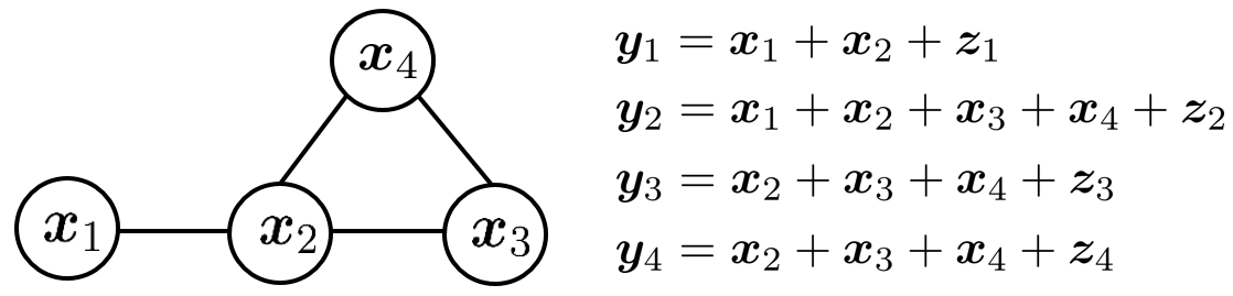
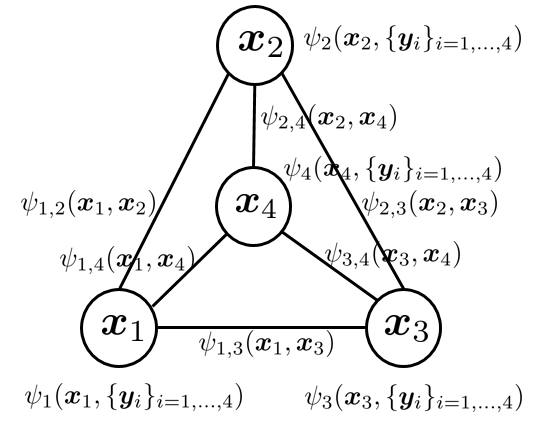
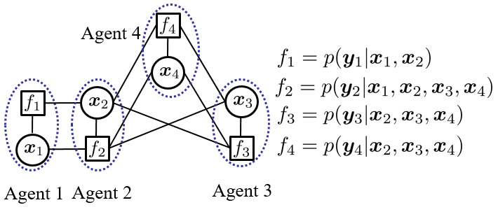
Figure 1: (a) A physical network with 4 agents, where $\left\{1,2\right\}$ and $\left\{2,3,4\right\}$ are two groups of agents that are within the communication range of each other, respectively. $\textbf{x}_{i}$ is the local unknown vector, and $\textbf{y}_{i}$ is the local observation at agent $i$ that follows (1); (b) The corresponding MRF of Fig. 1 (a) with $\psi_{n}\left(\textbf{x}_{n},\left\{\textbf{y}_{i}\right\}_{i\in n\cup\mathcal{I}(n)}\right)$ and $\psi_{n,i}\left(\textbf{x}_{n},\textbf{x}_{i}\right)$ defined in (6) and (7), respectively. (c) The corresponding factor graph of Fig. 1 (a) with $f_{i}$ defined in (10). Since $p(\textbf{x}_{i})$ does not involve message passing, the $p(\textbf{x}_{i})$ associated to each variable node is not drawn to keep the figure simple.

Secondly, even if the message scheduling between non-neighboring agents can be realized, the convergence of (8) is not guaranteed in loopy networks. For Gaussian MRF with scalar variables, sufficient convergence conditions have been proposed in (Weiss and Freeman, 2001a; Malioutov et al., 2006; Su and Wu, 2015). However, depending on how the factorization of the underlying joint Gaussian distribution is performed, Gaussian BP may exhibit different convergence properties as different factorizations (different Gaussian models) lead to fundamentally different recursive update structures. Furthermore, these results apply only to scalar Gaussian BP, and extension to vector-valued Gaussian BP is nontrivial as we show in this paper.

The next section derives distributed vector inference based on Gaussian BP with high order interactions (beyond pairwise connections), where information sharing and message exchange requirement conform to the physical network topology. Furthermore, convergence conditions will be studied in Section 4, and we show in Section 5 that the convergence condition obtained is strictly weaker than, i.e., subsumes the convergence conditions in (Weiss and Freeman, 2001a; Malioutov et al., 2006; Su and Wu, 2015).

3 Distributed Inference with Vector-Valued Gaussian BP and Non-Pairwise Interaction

The joint distribution $p\left(\textbf{x}\right)p\left(\textbf{y}|\textbf{x}\right)$ is first written as the product of the prior distribution and the likelihood function of each local linear Gaussian model in (1) as

$$p\left(\textbf{x}\right)p\left(\textbf{y}|\textbf{x}\right)=\prod_{n\in\mathcal{V}}p\left(\textbf{x}_{n}\right)\prod_{n\in\mathcal{V}}\underbrace{p\left(\textbf{y}_{n}|\left\{\textbf{x}_{i}\right\}_{i\in n\cup\mathcal{I}\left(n\right)}\right)}_{\triangleq f_{n}}.$$ (10)

To facilitate the derivation of the distributed inference algorithm, the factorization in (10) is expressed in terms of a factor graph (Kschischang et al., 2001), where every vector variable $\textbf{x}_{i}$ is represented by a circle (called variable node) and the probability distribution of a vector variable or a group of vector variables is represented by a square (called factor node). A variable node is connected to a factor node if the variable is involved in that particular factor. For example, Fig. 1(c) shows the factor graph representation for the network in Fig. 1(a).

We derive the Gaussian BP algorithm over the corresponding factor graph to learn $\textbf{x}_{n}$ for all $n\in\mathcal{V}$ (Kschischang et al., 2001). It involves two types of messages: one is the message from a variable node $\textbf{x}_{j}$ to its neighboring factor node $f_{n}$, defined as

$$m^{\left(\ell\right)}_{j\to f_{n}}\left(\textbf{x}_{j}\right)=p\left(\textbf{x}_{j}\right)\prod_{f_{k}\in\mathcal{B}(j)\setminus f_{n}}m^{\left(\ell-1\right)}_{f_{k}\to j}\left(\textbf{x}_{j}\right),$$ (11)

where $\mathcal{B}\left(j\right)$ denotes the set of neighbouring factor nodes of $\textbf{x}_{j}$, and $m^{\left(\ell-1\right)}_{f_{k}\to j}\left(\textbf{x}_{j}\right)$ is the message from $f_{k}$ to $\textbf{x}_{j}$ at time $\ell-1$. The second type of message is from a factor node $f_{n}$ to a neighboring variable node $\textbf{x}_{i}$, defined as

$$m^{\left(\ell\right)}_{f_{n}\to i}\left(\textbf{x}_{i}\right)=\int\cdots\int f_{n}\times\!\prod_{j\in\mathcal{B}\left(f_{n}\right)\setminus i}m^{\left(\ell\right)}_{j\to f_{n}}\left(\textbf{x}_{j}\right)\,\mathrm{d}\left\{\textbf{x}_{j}\right\}_{j\in{\mathcal{B}}\left(f_{n}\right)\setminus i},$$ (12)

where $\mathcal{B}\left(f_{n}\right)$ denotes the set of neighboring variable nodes of $f_{n}$. The process iterates between equations (11) and (12). At each iteration $\ell$, the approximate marginal distribution, also referred to as belief, on $\textbf{x}_{i}$ is computed locally at $\textbf{x}_{i}$ as

$$b_{\textrm{BP}}^{\left(\ell\right)}\left(\textbf{x}_{i}\right)=p\left(\textbf{x}_{i}\right)\prod_{f_{n}\in\mathcal{B}\left(i\right)}m^{\left(\ell\right)}_{f_{n}\to i}\left(\textbf{x}_{i}\right).$$ (13)

In the sequel, we derive the exact expressions for the messages $m^{\left(\ell\right)}_{j\to f_{n}}\left(\textbf{x}_{j}\right)$, $m^{\left(\ell\right)}_{f_{n}\to i}\left(\textbf{x}_{i}\right)$, and belief $b_{\textrm{BP}}^{\left(\ell\right)}\left(\textbf{x}_{i}\right)$. First, let the initial messages at each variable node and factor node be in Gaussian function forms as

$$m^{\left(0\right)}_{f_{n}\to i}\left(\textbf{x}_{i}\right)\propto\exp\left\{-\frac{1}{2}||\textbf{x}_{i}-\textbf{v}^{\left(0\right)}_{f_{n}\to i}||^{2}_{\textbf{J}^{\left(0\right)}_{f_{n}\to i}}\right\}.$$ (14)

In Appendix A, it is shown that the general expression for the message from variable node $j$ to factor node $f_{n}$ is

$$m^{\left(\ell\right)}_{j\to f_{n}}\left(\textbf{x}_{j}\right)\propto\exp\left\{-\frac{1}{2}||\textbf{x}_{j}-\textbf{v}^{\left(\ell\right)}_{j\to f_{n}}||^{2}_{\textbf{J}^{\left(\ell\right)}_{j\to f_{n}}}\right\},$$ (15)

with

$$\textbf{J}^{\left(\ell\right)}_{j\to f_{n}}=\textbf{W}_{j}^{-1}+\sum_{f_{k}\in{\mathcal{B}}\left(j\right)\setminus f_{n}}\textbf{J}_{f_{k}\to j}^{\left(\ell-1\right)},$$ (16)

$$\textbf{v}^{\left(\ell\right)}_{j\to f_{n}}=\left[\textbf{J}^{\left(\ell\right)}_{j\to f_{n}}\right]^{-1}\left[\sum_{f_{k}\in{\mathcal{B}}\left(j\right)\setminus f_{n}}\textbf{J}_{f_{k}\to j}^{\left(\ell-1\right)}\textbf{v}^{\left(\ell-1\right)}_{f_{k}\to j}\right],$$ (17)

where $\textbf{J}_{f_{k}\to j}^{\left(\ell-1\right)}$ and $\textbf{v}_{f_{k}\to j}^{\left(\ell-1\right)}$ are the message information matrix (inverse of covariance matrix) and mean vector received at variable node $j$ at the $\left(\ell-1\right)$-th iteration, respectively. Furthermore, the message from factor node $f_{n}$ to variable node $i$ is given by

$$m^{\left(\ell\right)}_{f_{n}\to i}\left(\textbf{x}_{i}\right)\propto\alpha_{f_{n}\to i}^{\left(\ell\right)}\exp\left\{-\frac{1}{2}||\textbf{x}_{i}-\textbf{v}^{\left(\ell\right)}_{f_{n}\to i}||^{2}_{\textbf{J}^{\left(\ell\right)}_{f_{n}\to i}}\right\},$$ (18)

with

$$\begin{split}\textbf{J}^{\left(\ell\right)}_{f_{n}\to i}=\textbf{A}_{n,i}^{T}\left[\textbf{R}_{n}+\sum_{j\in{\mathcal{B}}\left(f_{n}\right)\setminus i}\textbf{A}_{n,j}\left[\textbf{J}^{\left(\ell\right)}_{j\to f_{n}}\right]^{-1}\textbf{A}_{n,j}^{T}\right]^{-1}\textbf{A}_{n,i},\end{split}$$ (19)

$$\begin{split}\textbf{v}^{\left(\ell\right)}_{f_{n}\to i}=\left[\textbf{J}_{f_{n}\to i}^{\left(\ell\right)}\right]^{-1}\textbf{A}_{n,i}^{T}\left[\textbf{R}_{n}+\sum_{j\in{\mathcal{B}}\left(f_{n}\right)\setminus i}\textbf{A}_{n,j}\left[\textbf{J}^{\left(\ell\right)}_{j\to f_{n}}\right]^{-1}\textbf{A}_{n,j}^{T}\right]^{-1}\left(\textbf{y}_{n}-\sum_{j\in{\mathcal{B}}\left(f_{n}\right)\setminus i}\textbf{A}_{n,j}\textbf{v}^{\left(\ell\right)}_{j\to f_{n}}\right),\end{split}$$ (20)

and

$$\alpha_{f_{n}\to i}^{\left(\ell\right)}\propto\int\ldots\int\exp\left\{-\frac{1}{2}\textbf{z}^{T}\bm{\Lambda}_{f_{n}\to i}^{\left(\ell\right)}\textbf{z}\right\}\,\mathrm{d}\textbf{z}.$$ (21)

In (21), $\bm{\Lambda}_{f_{n}\to i}^{\left(\ell\right)}$ is a diagonal matrix containing the eigenvalues of $\textbf{A}_{n,\left\{{\mathcal{B}}\left(f_{n}\right)\setminus i\right\}}^{T}\textbf{R}_{n}^{-1}\textbf{A}_{n,\left\{{\mathcal{B}}\left(f_{n}\right)\setminus i\right\}}+\textbf{J}^{\left(\ell\right)}_{\left\{{\mathcal{B}}\left(f_{n}\right)\setminus i\right\}\to f_{n}}$, with $\textbf{A}_{n,\left\{{\mathcal{B}}\left(f_{n}\right)\setminus i\right\}}$ denoting a row block matrix containing $\textbf{A}_{n,j}$ as row elements for all $j\in{\mathcal{B}}\left(f_{n}\right)\setminus i$ arranged in ascending order, and $\textbf{J}^{\left(\ell\right)}_{\left\{{\mathcal{B}}\left(f_{n}\right)\setminus i\right\}\to f_{n}}$ denoting a block diagonal matrix with $\textbf{J}^{\left(\ell\right)}_{j\to f_{n}}$ as its block diagonal elements for all $j\in{\mathcal{B}}\left(f_{n}\right)\setminus i$ arranged in ascending order.

Obviously, the validity of (18) depends on the existence of $\alpha_{f_{n}\to i}^{\left(\ell\right)}$. It is evident that (21) is the integral of a Gaussian distribution and equals to a constant when $\bm{\Lambda}_{f_{n}\to i}^{\left(\ell\right)}\succ\textbf{0}$ or equivalently $\textbf{A}_{n,\left\{{\mathcal{B}}\left(f_{n}\right)\setminus i\right\}}^{T}\textbf{R}_{n}^{-1}\textbf{A}_{n,\left\{{\mathcal{B}}\left(f_{n}\right)\setminus i\right\}}+\textbf{J}^{\left(\ell\right)}_{\left\{{\mathcal{B}}\left(f_{n}\right)\setminus i\right\}\to f_{n}}\succ\textbf{0}.$ Otherwise, $\alpha_{f_{n}\to i}^{\left(\ell\right)}$ does not exist. Therefore, the necessary and sufficient condition for the existence of $m^{\left(\ell\right)}_{f_{n}\to i}\left(\textbf{x}_{i}\right)$ is

$$\textbf{A}_{n,\left\{{\mathcal{B}}\left(f_{n}\right)\setminus i\right\}}^{T}\textbf{R}_{n}^{-1}\textbf{A}_{n,\left\{{\mathcal{B}}\left(f_{n}\right)\setminus i\right\}}+\textbf{J}^{\left(\ell\right)}_{\left\{{\mathcal{B}}\left(f_{n}\right)\setminus i\right\}\to f_{n}}\succ\textbf{0}.$$ (22)

In general, the necessary and sufficient condition is difficult to be verified, as $\textbf{J}^{\left(\ell\right)}_{\left\{{\mathcal{B}}\left(f_{n}\right)\setminus i\right\}\to f_{n}}$ changes in each iteration. However, as $\textbf{R}_{n}^{-1}\succ\textbf{0}$, it can be decomposed as $\textbf{R}_{n}^{-1}=\widetilde{\textbf{R}}^{T}_{n}\widetilde{\textbf{R}}_{n}$. Then

$$\textbf{A}_{n,\left\{{\mathcal{B}}\left(f_{n}\right)\setminus i\right\}}^{T}\textbf{R}_{n}^{-1}\textbf{A}_{n,\left\{{\mathcal{B}}\left(f_{n}\right)\setminus i\right\}}=\left(\widetilde{\textbf{R}}_{n}\textbf{A}_{n,\left\{{\mathcal{B}}\left(f_{n}\right)\setminus i\right\}}\right)^{T}\left(\widetilde{\textbf{R}}_{n}\textbf{A}_{n,\left\{{\mathcal{B}}\left(f_{n}\right)\setminus i\right\}}\right)\succeq\textbf{0}.$$

Hence, one simple sufficient condition to guarantee (22) is $\textbf{J}^{\left(\ell\right)}_{\left\{{\mathcal{B}}\left(f_{n}\right)\setminus i\right\}\to f_{n}}\succ\textbf{0}$ or equivalently its diagonal block matrix $\textbf{J}^{\left(\ell\right)}_{j\to f_{n}}\succ\textbf{0}$ for all $j\in{\mathcal{B}}\left(f_{n}\right)\setminus i$. The following lemma shows that setting the initial message covariances $\textbf{J}_{f_{n}\to i}^{\left(0\right)}\succeq\textbf{0}$ for all $\left(n,i\right)\in\mathcal{E}_{\textrm{Net}}$ guarantees $\textbf{J}^{\left(\ell\right)}_{j\to f_{n}}\succ\textbf{0}$ for $\ell\geq 1$ and all $\left(n,j\right)\in\mathcal{E}_{\textrm{Net}}$.

Lemma 2

Let the initial messages at factor node $f_{k}$ be in Gaussian forms with the initial message information matrix $\textbf{J}_{f_{k}\to j}^{\left(0\right)}\succeq\textbf{0}$ for all $k\in\mathcal{V}$ and $j\in\mathcal{B}\left(f_{k}\right)$. Then $\textbf{J}_{j\to f_{n}}^{\left(\ell\right)}\succ\textbf{0}$ and $\textbf{J}^{\left(\ell\right)}_{f_{k}\to j}\succ\textbf{0}$ for all $\ell\geq 1$ with $j\in\mathcal{V}$ and $f_{n},f_{k}\in\mathcal{B}\left(j\right)$. Furthermore, in this case, all messages $m^{\left(\ell\right)}_{j\to f_{n}}\left(\textbf{x}_{j}\right)$ and $m^{\left(\ell\right)}_{f_{k}\to j}\left(\textbf{x}_{i}\right)$ are well defined.

Proof  See Appendix B.  

For this factor graph based approach, according to the message updating procedure (15) and (18), message exchange is only needed between neighboring agents (an agent refers to a variable-factor pair as shown in Fig. 1 (c)). For example, the messages transmitted from agent $n$ to its neighboring agent $i$ are $m_{f_{n}\to i}^{\left(\ell\right)}\left(\textbf{x}_{i}\right)$ and $m_{n\to f_{i}}^{\left(\ell\right)}\left(\textbf{x}_{n}\right)$. Thus, the factor graph does impose a clear messaging schedule, and the message passing scheme given in (11) and (12) conforms with the network topology. Furthermore, if the messages $m_{j\to f_{n}}^{\left(\ell\right)}\left(\textbf{x}_{j}\right)$ and $m_{f_{n}\to i}^{\left(\ell\right)}\left(\textbf{x}_{i}\right)$ exist for all $\ell$ (which can be achieved using Lemma 2), the messages are Gaussian, therefore only the corresponding mean vectors and information matrices (inverse of covariance matrices) are needed to be exchanged.

Finally, if the Gaussian BP messages exist, according to the definition of belief in (13), $b_{\textrm{BP}}^{\left(\ell\right)}\left(\textbf{x}_{i}\right)$ at iteration $\ell$ is computed as

$$\begin{split}\mathbf{b}_{\textrm{BP}}^{\left(\ell\right)}\left(\textbf{x}_{i}\right)&=p\left(\textbf{x}_{i}\right)\prod_{f_{n}\in\mathcal{B}\left(i\right)}m_{f_{n}\to i}^{\left(\ell\right)}\left(\textbf{x}_{i}\right),\\ &\propto\mathcal{N}\left(\textbf{x}_{i}|\bm{\mu}_{i}^{\left(\ell\right)},\textbf{P}_{i}^{\left(\ell\right)}\right),\end{split}$$

where the belief covariance matrix

$$\textbf{P}_{i}^{\left(\ell\right)}=\left[\textbf{W}_{i}^{-1}+\sum_{f_{n}\in{\mathcal{B}}\left(i\right)}\textbf{J}_{f_{n}\to i}^{\left(\ell\right)}\right]^{-1},$$ (23)

and mean vector

$$\bm{\mu}_{i}^{\left(\ell\right)}=\textbf{P}_{i}^{\left(\ell\right)}\left[\sum_{f_{n}\in{\mathcal{B}}\left(i\right)}\textbf{J}_{f_{n}\to i}^{\left(\ell\right)}\textbf{v}^{\left(\ell\right)}_{f_{n}\to i}\right].$$ (24)

The iterative algorithm based on Gaussian BP is summarized as follows. The algorithm is started by setting the messages from factor nodes to variable nodes as in (14). At each round of message exchange, every variable node computes the output messages to its neighboring factor nodes according to (16) and (17). After receiving the messages from its neighboring variable nodes, each factor node computes its output messages according to (19) and (20). The iterative computation terminates when the iterates in (15) or (18) tend to approach a fixed value or the maximum number of iterations is reached.

Remark 3

We assume that $\textbf{R}_{n}\succ\textbf{0}$ in this paper. If, however, some of the observations are noiseless, for example, $\textbf{R}_{n}=\textbf{0}$, the local observation is $\textbf{y}_{n}=\sum_{i\in n\cup\mathcal{I}\left(n\right)}\textbf{A}_{n,i}\textbf{x}_{i}$. Then the corresponding local likelihood function is represented by the Dirac measure $\delta(\textbf{y}_{n}-\sum_{i\in n\cup\mathcal{I}\left(n\right)}\textbf{A}_{n,i}\textbf{x}_{i})$. Suppose, for example, there is only one agent with $\textbf{R}_{n}=\textbf{0}$, and all others are $\textbf{R}_{i}\succ\textbf{0}$. The the joint distribution is written as

$$p\left(\textbf{x}\right)p\left(\textbf{y}|\textbf{x}\right)=\delta(\textbf{y}_{n}-\sum_{i\in n\cup\mathcal{I}\left(n\right)}\textbf{A}_{n,i}\textbf{x}_{i})\prod_{j\in\mathcal{V}}p\left(\textbf{x}_{j}\right)\prod_{k\in\mathcal{V}}{p\left(\textbf{y}_{k}|\left\{\textbf{x}_{i}\right\}_{i\in k\cup\mathcal{I}\left(k\right)}\right)}.$$

In this case, if $\textbf{A}_{n,n}$ is invertible, then, by the definition of the Dirac measure, we have $\textbf{x}_{n}=\textbf{A}_{n,n}^{-1}\left(\textbf{y}_{n}-\sum_{i\in\mathcal{I}\left(n\right)}\textbf{A}_{n,i}\textbf{x}_{i}\right)$. By substituting this equation into all of the likelihood functions involving $\textbf{x}_{n}$, we have the equivalent joint distribution as in (10) with all the likelihood functions having a positive definite noise covariance. We thereafter can apply Gaussian BP to this new factorization and the convergence analysis in this paper still applies. Therefore, without loss of generality, we assume all $\textbf{R}_{n}\succ\textbf{0}$. Note that when $\textbf{R}_{n}=\textbf{0}$ for all $n$, this problem is equivalent to solving algebraic equations, which has been studied in (Shental et al., 2008b) using Gaussian BP.

4 Convergence Analysis

The challenge of deploying the Gaussian BP algorithm for large-scale networks is in determining whether it will converge or not. In particular, it is generally known that if the factor graph contains cycles, the Gaussian BP algorithm may diverge. Thus, determining convergence conditions for the Gaussian BP algorithm is very important. Sufficient conditions for the convergence of Gaussian BP with scalar variables in loopy graphs are available in (Weiss and Freeman, 2001a; Malioutov et al., 2006; Su and Wu, 2015). However, these conditions are derived based on pairwise graphs with local functions in the form of (6) and (7). This contrasts with the model considered in this paper, where the $f_{n}$ in (10) involves high-order interactions between vector variables, and thus the convergence results in (Weiss and Freeman, 2001a; Malioutov et al., 2006; Su and Wu, 2015) cannot be applied to the factor graph based vector-form Gaussian BP.

Due to the recursive updating property of $m_{j\to f_{n}}^{\left(\ell\right)}\left(\textbf{x}_{j}\right)$ and $m_{f_{n}\to i}^{\left(\ell\right)}\left(\textbf{x}_{i}\right)$ in (15) and (18), the message evolution can be simplified by combining these two kinds of messages into one. By substituting $\textbf{J}^{\left(\ell\right)}_{j\to f_{n}}$ in (16) into (19), the updating of the message covariance matrix inverse, referred to as message information matrix in the following, can be denoted as

$$\textbf{J}_{f_{n}\to i}^{\left(\ell\right)} = \textbf{A}_{n,i}^{T}\bigg{[}\textbf{R}_{n}+\sum_{j\in{\mathcal{B}}\left(f_{n}\right)\setminus i}\textbf{A}_{n,j}\bigg{[}\textbf{W}_{j}^{-1}+\sum_{f_{k}\in{\mathcal{B}}\left(j\right)\setminus f_{n}}\textbf{J}_{f_{k}\to j}^{\left(\ell-1\right)}\bigg{]}^{-1}\textbf{A}_{n,j}^{T}\bigg{]}^{-1}\textbf{A}_{n,i}$$ (25)

$$\triangleq \mathcal{F}_{n\to i}\left(\left\{\textbf{J}_{f_{k}\to j}^{\left(\ell-1\right)}\right\}_{\left(f_{k},j\right)\in\mathcal{\widetilde{B}}\left(f_{n},i\right)}\right),$$

where $\mathcal{\widetilde{B}}\left(f_{n},i\right)=\left\{\left(f_{k},j\right)|j\in{\mathcal{B}}\left(f_{n}\right)\setminus i,f_{k}\in{\mathcal{B}}\left(j\right)\setminus f_{n}\right\}$. Observing that $\textbf{J}_{f_{n}\to i}^{\left(\ell\right)}$ in (25) is independent of $\textbf{v}^{\left(\ell\right)}_{j\to f_{n}}$ and $\textbf{v}^{\left(\ell\right)}_{f_{n}\to i}$ in (17) and (18), so we can first focus on the convergence property of $\textbf{J}_{f_{n}\to i}^{\left(\ell\right)}$ alone and then later on that of $\textbf{v}^{\left(\ell\right)}_{f_{n}\to i}$. With the convergence characterization of $\textbf{J}_{f_{n}\to i}^{\left(\ell\right)}$ and $\textbf{v}^{\left(\ell\right)}_{f_{n}\to i}$, we will further investigate the convergence of belief covariances and means in (23) and (24), respectively.

Note that computing $\textbf{P}_{j}^{(\ell)}$ requires all the incoming messages from neighboring nodes including $\textbf{J}_{f_{n}\to j}^{\left(\ell\right)}$ as shown in (23) by replacing the subscript $i$ with $j$ in (23). However, according to (25), when computing $\textbf{J}_{f_{n}\to i}^{\left(\ell\right)}$ the quantity $\textbf{J}_{f_{n}\to j}^{\left(\ell-1\right)}$ is excluded, i.e., the quantity inside the inner square brackets equals $[\textbf{P}_{j}^{\left(\ell-1\right)}]^{-1}-\textbf{J}_{f_{n}\to j}^{\left(\ell-1\right)}$. Therefore, one cannot compute $\textbf{J}_{f_{n}\to i}^{\left(\ell\right)}$ from $\textbf{P}_{j}^{(\ell)}$ alone.

4.1 Convergence of Message Information Matrices

To efficiently represent the updates of all message information matrices, we introduce the following definitions. Let

$${\textbf{J}}^{\left(\ell-1\right)}\triangleq\texttt{Bdiag}\left(\left\{\textbf{J}_{f_{n}\to i}^{\left(\ell-1\right)}\right\}_{n\in\mathcal{V},i\in{\mathcal{B}}\left(f_{n}\right)}\right)$$

be a block diagonal matrix with diagonal blocks being the message information matrices in the network at time $\ell-1$ with index arranged in ascending order first on $n$ and then on $i$. Using the definition of $\textbf{J}^{\left(\ell-1\right)}$, the term $\sum_{f_{k}\in\mathcal{B}\left(j\right)\backslash f_{n}}\textbf{J}_{f_{k}\rightarrow j}^{\left(\ell-1\right)}$ in (25) can be written as $\bm{\Xi}_{n,j}\textbf{J}^{\left(\ell-1\right)}\bm{\Xi}_{n,j}^{T}$, where $\bm{\Xi}_{n,j}$ is for selecting appropriate components from $\textbf{J}^{\left(\ell-1\right)}$ to form the summation. Further, define $\textbf{H}_{n,i}=\left[\left\{\textbf{A}_{n,j}\right\}_{j\in B\left(f_{n}\right)\backslash i}\right]$, $\bm{\Psi}_{n,i}=\texttt{Bdiag}\left(\left\{\textbf{W}_{j}^{-1}\right\}_{j\in B\left(f_{n}\right)\backslash i}\right)$ and $\textbf{K}_{n,i}=\texttt{Bdiag}\left(\left\{\bm{\Xi}_{n,j}\right\}_{j\in B\left(f_{n}\right)\backslash i}\right)$, all with component blocks arranged with ascending order on $j$. Then (25) can be written as

$$\textbf{J}^{\left(\ell\right)}_{f_{n}\rightarrow i}=\textbf{A}_{n,i}^{T}\left\{\textbf{R}_{n}+\textbf{H}_{n,i}\left[\bm{\Psi}_{n,i}+\textbf{K}_{n,i}\left(\textbf{I}_{|\mathcal{B}\left(f_{n}\right)|-1}\otimes\textbf{J}^{\left(\ell-1\right)}\right)\textbf{K}_{n,i}^{T}\right]^{-1}\textbf{H}_{n,i}^{T}\right\}^{-1}\textbf{A}_{n,i}.$$ (26)

Now, we define the function $\mathcal{F}\triangleq\left\{\mathcal{F}_{1\to k},\ldots,\mathcal{F}_{n\to i},\ldots,\mathcal{F}_{n\to M}\right\}$ that satisfies ${\textbf{J}}^{\left(\ell\right)}=\mathcal{F}\left({\textbf{J}}^{\left(\ell-1\right)}\right)$. Then, by stacking $\textbf{J}_{f_{n}\to i}^{\left(\ell\right)}$ on the left side of (26) for all $n$ and $i$ as the block diagonal matrix $\textbf{J}^{\left(\ell\right)}$, we obtain

$$\textbf{J}^{\left(\ell\right)} = \textbf{A}^{T}\big{\{}\bm{\Omega}+\textbf{H}\left[\bm{\Psi}+\textbf{K}\left(\mathbf{I}_{\varphi}\otimes\textbf{J}^{\left(\ell-1\right)}\right)\textbf{K}^{T}\right]^{-1}\textbf{H}^{T}\big{\}}^{-1}\textbf{A},$$ (27)

$$\triangleq \mathcal{F}\left(\textbf{J}^{\left(\ell-1\right)}\right),$$

where A, H, $\bm{\Psi}$, and K are block diagonal matrices with block elements $\textbf{A}_{n,i}$, $\textbf{H}_{n,i}$, $\bm{\Psi}_{n,i}$, and $\textbf{K}_{n,i}$, respectively, arranged in ascending order, first on $n$ and then on $i$ (i.e., the same order as $\textbf{J}^{\left(\ell\right)}_{f_{n}\rightarrow i}$ in $\textbf{J}^{\left(\ell\right)}$). Furthermore, $\varphi={\sum_{n=1}^{M}|\mathcal{B}\left(f_{n}\right)|\left(|\mathcal{B}\left(f_{n}\right)|-1\right)}$ and $\bm{\Omega}$ is a block diagonal matrix with diagonal blocks $\textbf{I}_{|B\left(f_{n}\right)|}\otimes\textbf{R}_{n}$ with ascending order on $n$. We first present some properties of the updating operator $\mathcal{F}\left(\cdot\right)$, the proofs being provided in Appendix C.

Proposition 4

The updating operator $\mathcal{F}\left(\cdot\right)$ satisfies the following properties:

P 4.1: $\mathcal{F}\left(\textbf{J}^{\left(\ell\right)}\right)\succeq\mathcal{F}\left(\textbf{J}^{\left(\ell-1\right)}\right)$, if $\textbf{J}^{\left(\ell\right)}\succeq\textbf{J}^{\left(\ell-1\right)}\succeq\textbf{0}$.

P 4.2: $\alpha\mathcal{F}\left(\textbf{J}^{\left(\ell\right)}\right)\succ\mathcal{F}\left(\alpha\textbf{J}^{\left(\ell\right)}\right)$ and $\mathcal{F}\left(\alpha^{-1}\textbf{J}^{\left(\ell\right)}\right)\succ\alpha^{-1}\mathcal{F}\left(\textbf{J}^{\left(\ell\right)}\right)$, if $\textbf{J}^{\left(\ell\right)}\succ\textbf{0}$ and $\alpha>1$.

P 4.3: Define $\textbf{U}\triangleq\textbf{A}^{T}\bm{\Omega}^{-1}\textbf{A}$ and $\textbf{L}\triangleq\textbf{A}^{T}\left[\bm{\Omega}+\textbf{H}\bm{\Psi}^{-1}\textbf{H}^{T}\right]^{-1}\textbf{A}$. With arbitrary $\textbf{J}^{\left(0\right)}\succeq\textbf{0}$, $\mathcal{F}\left(\textbf{J}^{\left(\ell\right)}\right)$ is bounded by $\textbf{U}\succeq\mathcal{F}\left(\textbf{J}^{\left(\ell\right)}\right)\succeq\textbf{L}\succ\textbf{0}$ for $\ell\geq 1$.

Based on the above properties of $\mathcal{F}\left(\cdot\right)$, we can establish the convergence of the information matrices.

Theorem 5

There exists a unique positive definite fixed point $\textbf{J}^{\ast}$ for the mapping $\mathcal{F}\left(\cdot\right)$.

Proof  The set $\left[\textbf{L},\textbf{U}\right]$ is a compact set. Further, according to Proposition 4, P 4.3, for arbitrary $\textbf{J}^{\left(0\right)}\succeq\textbf{0}$, $\mathcal{F}$ maps $\left[\textbf{L},\textbf{U}\right]$ into itself starting from $\ell\geq 1$. Next, we show that $\left[\textbf{L},\textbf{U}\right]$ is a convex set. Suppose that X, $\textbf{Y}\in\left[\textbf{L},\textbf{U}\right]$, and $0\leq t\leq 1$, then $t\textbf{X}-t\textbf{L}$ and $\left(1-t\right)\textbf{Y}-\left(1-t\right)\textbf{L}$ are positive semidefinite (p.s.d.) matrices. Since the sum of two p.s.d. matrices is a p.s.d. matrix, $t\textbf{X}+\left(1-t\right)\textbf{Y}\succeq\textbf{L}$. Likewise, it can be shown that $t\textbf{X}+\left(1-t\right)\textbf{Y}\preceq\textbf{U}$. Thus, the continuous function $\mathcal{F}$ maps a compact convex subset of the Banach space of positive definite matrices into itself. Therefore, the mapping $\mathcal{F}$ has a fixed point in $\left[\textbf{L},\textbf{U}\right]$ according to Brouwer’s Fixed-Point Theorem (Zeidler, 1985), and the fixed point is positive definite (p.d.).

Next, we prove the uniqueness of the fixed point. Suppose that there exist two fixed points $\textbf{J}^{\ast}\succ\textbf{0}$ and $\widetilde{\textbf{J}}^{\ast}\succ\textbf{0}$. Since $\textbf{J}^{\ast}$ and $\widetilde{\textbf{J}}^{\ast}$ are p.d., their components $\textbf{J}_{f_{n}\to i}^{\ast}$ and $\widetilde{\textbf{J}}_{f_{n}\to i}^{\ast}$ are also p.d. matrices. For the component blocks of $\textbf{J}^{\ast}$ and $\widetilde{\textbf{J}}^{\ast}$, there are two possibilities: 1) $\widetilde{\textbf{J}}_{f_{n}\to i}^{\ast}-\textbf{J}_{f_{n}\to i}^{\ast}\succ\textbf{0}$ or $\widetilde{\textbf{J}}_{f_{n}\to i}^{\ast}-\textbf{J}_{f_{n}\to i}^{\ast}$ is indefinite for some $n,i\in\mathcal{V}$, and 2) $\widetilde{\textbf{J}}^{\ast}_{f_{n}\to i}-\textbf{J}^{\ast}_{f_{n}\to i}\preceq 0$ for all $n,i\in\mathcal{V}$.

For the first case, there must exist $\xi_{f_{n},i}>1$ such that $\xi_{f_{n},i}\textbf{J}_{f_{n}\to i}^{\ast}-\widetilde{\textbf{J}}_{f_{n}\to i}^{\ast}$ has one or more zero eigenvalues, while all other eigenvalues are positive. Pick the component matrix with the maximum $\xi_{f_{n},i}$ among those falling into this case, say $\xi_{f_{\varrho},\tau}$, then, we can write

$$\xi_{f_{\varrho},\tau}\textbf{J}_{f_{\varrho}\to\tau}^{\ast}-\widetilde{\textbf{J}}_{f_{\varrho}\to\tau}^{\ast}\succeq\textbf{0},$$ (28)

or in terms of the information matrices for the whole network

$$\xi_{f_{\varrho},\tau}\textbf{J}^{\ast}\succeq\widetilde{\textbf{J}}^{\ast}\succ\textbf{0},\quad\xi_{f_{\varrho},\tau}>1.$$ (29)

Applying $\mathcal{F}$ on both sides of (29), according to the monotonic property of $\mathcal{F}\left(\cdot\right)$ as shown in Proposition 4, P 4.1, we have

$$\mathcal{F}\left(\xi_{f_{\varrho},\tau}\textbf{J}^{\ast}\right)\succeq\mathcal{F}\left(\widetilde{\textbf{J}}^{\ast}\right)=\widetilde{\textbf{J}}^{\ast},$$ (30)

where the equality is due to $\widetilde{\textbf{J}}^{\ast}$ being a fixed point. According to Proposition 4, P 4.2, $\xi_{f_{\varrho},\tau}\mathcal{F}\left(\textbf{J}^{\ast}\right)\succ\mathcal{F}\left(\xi_{f_{\varrho},\tau}\textbf{J}^{\ast}\right)$. Therefore, from (30), we obtain $\xi_{f_{\varrho,\tau}}\textbf{J}^{\ast}\succ\widetilde{\textbf{J}}^{\ast}$. Consequently,

$$\xi_{f_{\varrho,\tau}}\textbf{J}_{f_{\varrho,\tau}}^{\ast}\succ\widetilde{\textbf{J}}_{f_{\varrho,\tau}}^{\ast}.$$

But this contradicts with $\xi_{f_{\varrho},\tau}\textbf{J}_{f_{\varrho,\tau}}^{\ast}-\widetilde{\textbf{J}}_{f_{\varrho,\tau}}^{\ast}$ having one or more zero eigenvalues as discussed before (28). Therefore, we must have $\textbf{J}^{\ast}=\widetilde{\textbf{J}}^{\ast}$.

On the other hand, if we have case two, which is $\widetilde{\textbf{J}}^{\ast}_{f_{n}\to i}-\textbf{J}^{\ast}_{f_{n}\to i}\preceq 0$ for all $n,i\in\mathcal{V}$, we can repeat the above derivation with the roles of $\widetilde{\textbf{J}}^{\ast}$ and $\textbf{J}^{\ast}$ reversed, and we would again obtain $\textbf{J}^{\ast}=\widetilde{\textbf{J}}^{\ast}$. Consequently, $\textbf{J}^{\ast}$ is unique.  

Lemma 2 states that with arbitrary p.s.d. initial message information matrices, the message information matrices will be kept as p.d. at every iteration. On the other hand, Theorem 5 indicates that there exists a unique fixed point for the mapping $\mathcal{F}$. Next, we will show that, with arbitrary initial value $\textbf{J}^{\left(0\right)}\succeq 0$, $\textbf{J}^{\left(\ell\right)}$ converges to a unique p.d. matrix.

Theorem 6

The matrix sequence $\left\{\textbf{J}^{\left(\ell\right)}\right\}_{l=0,1,\ldots}$ defined by (27) converges to a unique positive definite matrix $\textbf{J}^{\ast}$ for any initial covariance matrix $\textbf{J}^{\left(0\right)}\succeq\mathbf{0}$.

Proof  With arbitrary initial value $\textbf{J}^{\left(0\right)}\succeq\textbf{0}$, following Proposition 4, P 4.3, we have $\textbf{U}\succeq\textbf{J}^{\left(1\right)}\succeq\textbf{L}\succ\textbf{0}$. On the other hand, according to Theorem 5, (27) has a unique fixed point $\textbf{J}^{\ast}\succ\textbf{0}$. Notice that we can always choose a scalar $\alpha>1$ such that

$$\alpha\textbf{J}^{\ast}\succeq\textbf{J}^{\left(1\right)}\succeq\textbf{L}.$$ (31)

Applying $\mathcal{F}\left(\cdot\right)$ to (31) $\ell$ times, and using Proposition 4, P 4.1, we have

$$\mathcal{F}^{\ell}\left(\alpha\textbf{J}^{\ast}\right)\succeq\mathcal{F}^{\ell+1}\left(\textbf{J}^{\left(0\right)}\right)\succeq\mathcal{F}^{\ell}\left(\textbf{L}\right),$$ (32)

where $\mathcal{F}^{\ell}\left(\textbf{X}\right)$ denotes applying $\mathcal{F}$ on X $\ell$ times.

We start from the left inequality in (32). According to Proposition 4, P 4.2, $\alpha\textbf{J}^{\ast}\succ\mathcal{F}\left(\alpha\textbf{J}^{\ast}\right)$. Applying $\mathcal{F}$ again gives $\mathcal{F}\left(\alpha\textbf{J}^{\ast}\right)\succ\mathcal{F}^{2}\left(\alpha\textbf{J}^{\ast}\right)$. Applying $\mathcal{F}\left(\cdot\right)$ repeatedly, we can obtain $\mathcal{F}^{2}\left(\alpha\textbf{J}^{\ast}\right)\succ\mathcal{F}^{3}\left(\alpha\textbf{J}^{\ast}\right)\succ\mathcal{F}^{4}\left(\alpha\textbf{J}^{\ast}\right)$, etc. Thus $\mathcal{F}^{\ell}\left(\alpha\textbf{J}^{\ast}\right)$ is a non-increasing sequence with respect to the partial order induced by the cone of p.s.d. matrices as $\ell$ increases. Furthermore, since $\mathcal{F}\left(\cdot\right)$ is bounded below by L, $\mathcal{F}^{\ell}\left(\alpha\textbf{J}^{\ast}\right)$ converges. Finally, since there exists only one fixed point for $\mathcal{F}\left(\cdot\right)$, $\lim_{l\to\infty}\mathcal{F}^{\ell}\left(\alpha\textbf{J}^{\ast}\right)=\textbf{J}^{\ast}$. On the other hand, for the right hand side of (32), as $\mathcal{F}\left(\cdot\right)\succeq\textbf{L}$, we have $\mathcal{F}\left(\textbf{L}\right)\succeq\textbf{L}$. Applying $\mathcal{F}$ repeatedly gives successively $\mathcal{F}^{2}\left(\textbf{L}\right)\succeq\mathcal{F}\left(\textbf{L}\right)$, $\mathcal{F}^{3}\left(\textbf{L}\right)\succeq\mathcal{F}^{2}\left(\textbf{L}\right)$, etc. So, $\mathcal{F}^{\ell}\left(\textbf{L}\right)$ is an non-decreasing sequence (with respect to the partial order induced by the cone of p.s.d. matrices). Since $\mathcal{F}\left(\cdot\right)$ is upper bounded by U, $\mathcal{F}^{\ell}\left(\textbf{L}\right)$ is a convergent sequence. Again, due to the uniqueness of the fixed point, we have $\lim_{l\to\infty}\mathcal{F}^{\ell}\left(\textbf{L}\right)=\textbf{J}^{\ast}$. Finally, taking the limit with respect to $\ell$ on (32), we have $\lim_{l\to\infty}\mathcal{F}^{\ell}\left(\textbf{J}^{\left(0\right)}\right)=\textbf{J}^{\ast},$ for arbitrary initial $\textbf{J}^{\left(0\right)}\succeq\mathbf{0}$.  

Remark 7

According to Theorem 6, the information matrix $\textbf{J}^{\left(\ell\right)}_{f_{n}\to i}$ converges if all initial information matrices are p.s.d., i.e., $\textbf{J}^{\left(0\right)}_{f_{n}\to i}\succeq\textbf{0}$ for all $i\in\mathcal{V}$ and $f_{n}\in\mathcal{B}\left(i\right)$. However, for the pairwise model, the messages are derived based on the classical Gaussian MRF based factorization (in the form of equations (6) and (7)) of the joint distribution. This differs from the model considered in this paper, where the factor $f_{n}$ follows equation (10), which leads to intrinsically different recursive equations. More specifically, for BP on the Gaussian MRF based factorization, the information matrix does not necessarily converge for all initial nonnegative values (for the scalar variable case) as shown in (Malioutov et al., 2006; Moallemi and Roy, 2009a).

Remark 8

Due to the computation of $\textbf{J}^{\left(\ell\right)}_{f_{n}\to i}$ being independent of the local observations $\textbf{y}_{n}$, as long as the network topology does not change, the converged value $\textbf{J}^{\ast}_{f_{n}\to i}$ can be precomputed offline and stored at each agent, and there is no need to re-compute $\textbf{J}^{\ast}_{f_{n}\to i}$ even if $\textbf{y}_{n}$ varies.

Another fundamental question is how fast the convergence is, and this is the focus of the discussion below. Since the convergence of a dynamic system is often studied with respect to the part metric (Chueshov, 2002), in the following, we start by introducing the part metric.

Definition 9

Part (Birkhoff) Metric (Chueshov, 2002): For arbitrary symmetric matrices X and Y with the same dimension, if there exists $\alpha\geq 1$ such that $\alpha\textbf{X}\succeq\textbf{Y}\succeq\alpha^{-1}\textbf{X}$, X and Y are called the parts, and $\mathrm{d}\left(\textbf{X},\textbf{Y}\right)\triangleq\inf\left\{\log\alpha:\alpha\textbf{X}\succeq\textbf{Y}\succeq\alpha^{-1}\textbf{X},\alpha\geq 1\right\}$ defines a metric called the part metric.

As it is useful to have an estimate of the convergence rate of $\textbf{J}^{\left(\ell\right)}$ in terms of the more standard induced matrix norms, we further introduce the notion of monotone norms. The norms $||\cdot||_{2}$ and $||\cdot||_{F}$ (Frobenus norm) are monotone norms.

Definition 10

Monotone Norm (Ciarlet, 1989, 2.2-10): A matrix norm $\|\cdot\|$ is monotone if

$$\textbf{X}\succeq\textbf{0},\textbf{Y}\succeq\textbf{X}\Rightarrow\|\textbf{Y}\|\geq\|\textbf{X}\|.$$

Next, for arbitrary $\epsilon>0$, we will show that $\left\{\textbf{J}^{\left(\ell\right)}\right\}_{l=1,..}$ approaches the $\epsilon$-neighborhood of the fixed point $\textbf{J}^{\star}$ double exponentially fast with respect to the monotone norm. To this end, for a fixed $\epsilon>0$, define the set

$$\mathcal{C}=\left\{\textbf{J}^{\left(\ell\right)}|\textbf{U}\succeq\textbf{J}^{\left(\ell\right)}\succeq\textbf{J}^{\ast}+\epsilon\textbf{I}\right\}\cup\left\{\textbf{J}^{\left(\ell\right)}|\textbf{J}^{\ast}-\epsilon\textbf{I}\succeq\textbf{J}^{\left(\ell\right)}\succeq\textbf{L}\right\}.$$ (33)

Theorem 11

With the initial message information matrix set to be an arbitrary p.s.d. matrix, i.e., $\textbf{J}^{\left(0\right)}_{f_{n}\to i}\succeq\textbf{0}$, the sequence $\left\{\textbf{J}^{\left(\ell\right)}\right\}_{l=0,1,\ldots}$ approaches an arbitrarily small neighborhood of the fixed positive definite matrix $\textbf{J}^{\ast}$ at a doubly exponential rate with respect to any matrix norm.

Proof  Fix $\epsilon>0$ and consider the set $\mathcal{C}$ defined in (33). It suffices to show that the quantity $\|\textbf{J}^{(\ell)}-\textbf{J}^{\ast}\|$, where $\|\cdot\|$ is a monotone norm as defined in Definition 10, decays double exponentially as long as $\textbf{J}^{(s)}\in\mathcal{C}$ for all $s\in\{0,1,\cdots\ell\}$. To this end, for $\textbf{J}^{\left(\ell\right)}\in\mathcal{C}$, and $\textbf{J}^{\ast}\not\in\mathcal{C}$ (necessarily), according to Definition 9, we have $\mathrm{d}\left(\textbf{J}^{\left(\ell\right)},\textbf{J}^{\ast}\right)\triangleq\inf\left\{\log\alpha:\alpha\textbf{J}^{\left(\ell\right)}\succeq\textbf{J}^{\ast}\succeq\alpha^{-1}\textbf{J}^{\left(\ell\right)}\right\}$. Since $\mathrm{d}\left(\textbf{J}^{\left(\ell\right)},\textbf{J}^{\ast}\right)$ is the smallest number satisfying $\alpha\textbf{J}^{\left(\ell\right)}\succeq\textbf{J}^{\ast}\succeq\alpha^{-1}\textbf{J}^{\left(\ell\right)}$, this is equivalent to

$$\exp\left\{\mathrm{d}\left(\textbf{J}^{\left(\ell\right)},\textbf{J}^{\ast}\right)\right\}\textbf{J}^{\left(\ell\right)}\succeq\textbf{J}^{\ast}\succeq\exp\left\{-\mathrm{d}\left(\textbf{J}^{\left(\ell\right)},\textbf{J}^{\ast}\right)\right\}\textbf{J}^{\left(\ell\right)}.$$ (34)

Applying Proposition 4, P 4.1 to (34), we have

$$\mathcal{F}\left(\exp\left\{\mathrm{d}\left(\textbf{J}^{\left(\ell\right)},\textbf{J}^{\ast}\right)\right\}\textbf{J}^{\left(\ell\right)}\right)\succ\mathcal{F}\left(\textbf{J}^{\ast}\right)\succ\mathcal{F}\left(\exp\left\{-\mathrm{d}\left(\textbf{J}^{\left(\ell\right)},\textbf{J}^{\ast}\right)\right\}\textbf{J}^{\left(\ell\right)}\right).$$

Then applying Proposition 4, P 4.2 and considering that $\exp\left\{\mathrm{d}\left(\textbf{J}^{\left(\ell\right)},\textbf{J}^{\ast}\right)\right\}>1$ and $\exp\left\{-\mathrm{d}\left(\textbf{J}^{\left(\ell\right)},\textbf{J}^{\ast}\right)\right\}<1$, we obtain

$$\exp\left\{\mathrm{d}\left(\textbf{J}^{\left(\ell\right)},\textbf{J}^{\ast}\right)\right\}\mathcal{F}\left(\textbf{J}^{\left(\ell\right)}\right)\succeq\mathcal{F}\left(\textbf{J}^{\ast}\right)\succeq\exp\left\{-\mathrm{d}\left(\textbf{J}^{\left(\ell\right)},\textbf{J}^{\ast}\right)\right\}\mathcal{F}\left(\textbf{J}^{\left(\ell\right)}\right).$$

Notice that, for arbitrary p.d. matrices X and Y, if $\textbf{X}-k\textbf{Y}\succ\textbf{0}$, then, by definition, we have $\textbf{x}^{T}\textbf{X}\textbf{x}-k\textbf{x}^{T}\textbf{Y}\textbf{x}>{0}$ for arbitrary $\textbf{x}\neq\textbf{0}$. Then, there must exist $o>0$ that is small enough such that $\textbf{x}^{T}\textbf{X}\textbf{x}-\left(k+o\right)\textbf{x}^{T}\textbf{Y}\textbf{x}>{0}$ or equivalently $\textbf{X}\succ\left(k+o\right)\textbf{Y}$. Thus, as $\exp{\left(\cdot\right)}$ is a continuous function, there must exist some $\triangle\mathrm{d}>0$ such that

$$\exp\left\{-\triangle\mathrm{d}+\mathrm{d}\left(\textbf{J}^{\left(\ell\right)},\textbf{J}^{\ast}\right)\right\}\mathcal{F}\left(\textbf{J}^{\left(\ell\right)}\right)\succ\mathcal{F}\left(\textbf{J}^{\ast}\right)\succ\exp\left\{\triangle\mathrm{d}-\mathrm{d}\left(\textbf{J}^{\left(\ell\right)},\textbf{J}^{\ast}\right)\right\}\mathcal{F}\left(\textbf{J}^{\left(\ell\right)}\right).$$ (35)

Now, using the definition of the part metric, (35) is equivalent to

$$-\triangle\mathrm{d}+\mathrm{d}\left(\textbf{J}^{\left(\ell\right)},\textbf{J}^{\ast}\right)\geq\mathrm{d}\left(\mathcal{F}\left(\textbf{J}^{\left(\ell\right)}\right),\mathcal{F}\left(\textbf{J}^{\ast}\right)\right).$$

Hence, we obtain $\mathrm{d}\left(\mathcal{F}\left(\textbf{J}^{\left(\ell\right)}\right),\mathcal{F}\left(\textbf{J}^{\ast}\right)\right)<\mathrm{d}\left(\textbf{J}^{\left(\ell\right)},\textbf{J}^{\ast}\right)$. Since this result holds for any $\textbf{J}^{\left(\ell\right)}\in\mathcal{C}$, we also have $\mathrm{d}\left(\mathcal{F}\left(\textbf{J}^{\left(\ell\right)}\right),\mathcal{F}\left(\textbf{J}^{\ast}\right)\right)<c\mathrm{d}\left(\textbf{J}^{\left(\ell\right)},\textbf{J}^{\ast}\right)$, where $c=\sup_{\textbf{J}^{(\ell)}\in\mathcal{C}}\frac{\mathrm{d}\left(\mathcal{F}\left(\textbf{J}^{(\ell)}\right),\mathcal{F}\left(\textbf{J}^{\ast}\right)\right)}{\mathrm{d}\left(\textbf{J}^{(\ell)},\textbf{J}^{\ast}\right)}<1$. Since $\textbf{J}^{\ell+1}=\mathcal{F}\left(\textbf{J}^{\ell}\right)$ and $\textbf{J}^{\ast}=\mathcal{F}\left(\textbf{J}^{\ast}\right)$, we have

$$\mathrm{d}\left(\textbf{J}^{\left(\ell\right)},\textbf{J}^{\ast}\right)<c^{\ell}\mathrm{d}\left(\textbf{J}^{\left(0\right)},\textbf{J}^{\ast}\right).$$ (36)

According to (Krause and Nussbaum, 1993, Lemma 2.3), the convergence rate of $||\textbf{J}^{\left(\ell\right)}-\textbf{J}^{\ast}||$ can be determined by that of $\mathrm{d}\left(\textbf{J}^{\left(\ell\right)},\textbf{J}^{\ast}\right)$. More specifically,

$$||\textbf{J}^{\left(\ell\right)}-\textbf{J}^{\ast}||\leq\left(2\exp\left\{\mathrm{d}\left(\textbf{J}^{\left(\ell\right)},\textbf{J}^{\ast}\right)\right\}-\exp\left\{-\mathrm{d}\left(\textbf{J}^{\left(\ell\right)},\textbf{J}^{\ast}\right)\right\}-1\right)\min\left\{||\textbf{J}^{\left(\ell\right)}||,||\textbf{J}^{\ast}||\right\},$$ (37)

where $||\cdot||$ is a monotone norm defined on the p.s.d. cone:

As we show in Proposition 4, P 4.3 that $\textbf{J}^{\left(\ell\right)}$ is bounded, then $||\textbf{J}^{\left(\ell\right)}||$ and $||\textbf{J}^{\ast}||$ must be finite. Let $\zeta$ be the largest value of $\min\left\{||\textbf{J}^{\left(\ell\right)}||,||\textbf{J}^{\ast}||\right\}$ for all $\{\textbf{J}^{\left(\ell\right)}\}$ with $\ell\geq 0$, then $\zeta>0$. According to (36) and (37), we have that

$$||\textbf{J}^{\left(\ell\right)}-\textbf{J}^{\ast}||<\zeta\left(2\exp\left\{c^{\ell}d_{0}\right\}-\exp\left\{-c^{\ell}d_{0}\right\}-1\right),$$ (38)

with $0<c<1$ and $d_{0}=\mathrm{d}\left(\textbf{J}^{\left(0\right)},\textbf{J}^{\ast}\right)$, which is a constant. The above inequality is equivalent to

$$||\textbf{J}^{\left(\ell\right)}-\textbf{J}^{\ast}||<\zeta\left(3\exp\left\{c^{\ell}d_{0}\right\}-\exp\left\{c^{\ell}d_{0}\right\}-\exp\left\{-c^{\ell}d_{0}\right\}-1\right).$$ (39)

Since both $\exp\left\{c^{\ell}d_{0}\right\}$ and $\exp\left\{-c^{\ell}d_{0}\right\}$ are positive and $\exp\left\{c^{\ell}d_{0}\right\}\exp\left\{-c^{\ell}d_{0}\right\}=1$, according to the arithmetic-geometric mean inequality, we have $\exp\left\{c^{\ell}d_{0}\right\}+\exp\left\{-c^{\ell}d_{0}\right\}\geq 2\left(\exp\left\{c^{\ell}d_{0}\right\}\exp\left\{-c^{\ell}d_{0}\right\}\right)^{1/2}=2$. Then, the right-hand side of (39) is further amplified, and we obtain

$$||\textbf{J}^{\left(\ell\right)}-\textbf{J}^{\ast}||<\zeta\left(3\exp\left\{c^{\ell}d_{0}\right\}-3\right)=3\zeta\left(\exp\left\{c^{\ell}d_{0}\right\}-1\right).$$

Therefore, the sequence $\left\{\textbf{J}^{\left(\ell\right)}\right\}_{l=0,1,\ldots}$ approaches the $\epsilon$-neighborhood (and hence any arbitrarily small neighborhood) of the fixed positive definite matrix $\textbf{J}^{\ast}$ at a doubly exponential rate with respect to any matrix norm.  
The physical meaning of Theorem 11 is that the distance between $\textbf{J}^{\left(\ell\right)}$ and $\textbf{J}^{\ast}$ decreases doubly exponentially fast before $\textbf{J}^{\left(\ell\right)}$ enters $\textbf{J}^{\ast}$’s neighborhood, which can be chosen to be arbitrarily small. Next, we study how to choose the initial value $\textbf{J}^{\left(0\right)}$ so that $\textbf{J}^{\left(\ell\right)}$ converges faster.

Theorem 12

With $\textbf{0}\preceq\textbf{J}^{\left(0\right)}\preceq\textbf{L}$, $\textbf{J}^{\left(\ell\right)}$ is a monotonic increasing sequence, and $\textbf{J}^{\left(\ell\right)}$ converges most rapidly with $\textbf{J}^{\left(0\right)}=\textbf{L}$. Moreover, with $\textbf{J}^{\left(0\right)}\succeq\textbf{U}$, $\textbf{J}^{\left(\ell\right)}$ is a monotonic decreasing sequence, and $\textbf{J}^{\left(\ell\right)}$ converges most rapidly with $\textbf{J}^{\left(0\right)}=\textbf{U}$.

Proof  Following Proposition 4, P 4.3, it can be verified that for $\textbf{0}\preceq\textbf{J}^{\left(0\right)}\preceq\textbf{L}$, we have $\textbf{J}^{\left(1\right)}\succeq\textbf{J}^{\left(0\right)}$. Then, according to Proposition 4, P 4.1, and by induction, this relationship can be extended to ${\textbf{J}}^{\left(\ell\right)}\succeq\ldots{\textbf{J}}^{\left(1\right)}\succeq{\textbf{J}}^{\left(0\right)}$, which states that ${\textbf{J}}^{\left(\ell\right)}$ is a monotonic increasing sequence. Now, suppose that there are two sequences $\textbf{J}^{\left(\ell\right)}$ and $\widetilde{\textbf{J}}^{\left(\ell\right)}$ that are started with different initial values $\textbf{0}\preceq\textbf{J}^{\left(0\right)}\prec\textbf{L}$ and $\textbf{0}\preceq\widetilde{\textbf{J}}^{\left(0\right)}\prec\textbf{L}$, respectively. Then these two sequences are monotonically increasing and bounded by $\textbf{J}^{\ast}$. To prove that $\textbf{J}^{\left(0\right)}=\textbf{L}$ leads to the fastest convergence, it is sufficient to prove that $\textbf{J}^{\left(\ell\right)}\succ\widetilde{\textbf{J}}^{\left(\ell\right)}$ for $\ell=0,1\ldots$. First, note that $\textbf{J}^{\left(0\right)}\succ\widetilde{\textbf{J}}^{\left(0\right)}$. Assume $\textbf{J}^{\left(n\right)}\succ\widetilde{\textbf{J}}^{\left(n\right)}$ for some $n\geq 0$. According to Proposition 4, P 4.1, we have $\mathcal{F}\left(\textbf{J}^{\left(n\right)}\right)\succeq\mathcal{F}\left(\widetilde{\textbf{J}}^{\left(n\right)}\right)$, or equivalently $\textbf{J}^{\left(n+1\right)}\succeq\widetilde{\textbf{J}}^{\left(n+1\right)}$. Therefore, by induction, we have proven that, with $\textbf{J}^{\left(0\right)}=\textbf{L}$, $\textbf{J}^{\left(\ell\right)}$ converges more rapidly than with any other initial value $\textbf{0}\preceq\textbf{J}^{\left(0\right)}\prec\textbf{L}$.

With similar logic, we can show that, with $\textbf{J}^{\left(0\right)}\succeq\textbf{U}$, $\textbf{J}^{\left(\ell\right)}$ is a monotonic decreasing sequence; and, with $\textbf{J}^{\left(0\right)}=\textbf{U}$, $\textbf{J}^{\left(\ell\right)}$ converges more rapidly than that with any other initial value $\textbf{J}^{\left(0\right)}\succ\textbf{U}$.  

Notice that it is a common practice in the Gaussian BP literature that the initial information matrix (or inverse variance for the scalar case) is set to be 0, i.e., $\textbf{J}^{\left(0\right)}_{f_{n}\to i}=\mathbf{0}$ (Weiss and Freeman, 2001a; Malioutov et al., 2006). Theorem 12 reveals that there is a better choice to guarantee faster convergence.

4.2 Convergence of Message Mean Vector

According to Theorems 6 and 11, as long as we choose $\textbf{J}_{f_{k}\to j}^{\left(0\right)}\succeq\textbf{0}$ for all $j\in\mathcal{V}$ and $f_{k}\in\mathcal{B}\left(j\right)$, the distance between $\textbf{J}_{f_{k}\to j}^{\left(\ell\right)}$ and $\textbf{J}_{f_{k}\to j}^{\ast}$ decreases doubly exponentially fast before $\textbf{J}_{f_{k}\to j}^{\left(\ell\right)}$ enters $\textbf{J}_{f_{k}\to j}^{\ast}$’s neighborhood, which can be chosen to be arbitrarily small. Furthermore, according to (16), $\left[\textbf{J}^{\left(\ell\right)}_{j\to f_{n}}\right]^{-1}$ also converges to a p.d. matrix once $\textbf{J}_{f_{k}\to j}^{\left(\ell\right)}$ converges, and the converged value for $\left[\textbf{J}^{\left(\ell\right)}_{j\to f_{n}}\right]^{-1}$ is denoted by $\left[\textbf{J}^{\ast}_{j\to f_{n}}\right]^{-1}$. Then for arbitrary initial value $\textbf{v}^{\left(0\right)}_{f_{k}\to j}$, the evolution of $\textbf{v}^{\left(\ell\right)}_{j\to f_{n}}$ in (17) can be written in terms of the converged message information matrices, which is

$$\textbf{v}^{\left(\ell\right)}_{j\to f_{n}}=\left[\textbf{J}^{\ast}_{j\to f_{n}}\right]^{-1}\sum_{f_{k}\in{\mathcal{B}}\left(j\right)\setminus f_{n}}\textbf{J}_{f_{k}\to j}^{\ast}\textbf{v}^{\left(\ell-1\right)}_{f_{k}\to j}.$$ (40)

Using (20), and replacing indices $j$, $i$, $n$ with $z$, $j$, $k$ respectively, $\textbf{v}^{\left(\ell-1\right)}_{f_{k}\to j}$ is given by

$$\begin{split}\textbf{v}^{\left(\ell-1\right)}_{f_{k}\to j}=[\textbf{J}_{f_{k}\to j}^{\ast}]^{-1}\textbf{A}_{k,j}^{T}\Bigg{[}\underbrace{\textbf{R}_{k}+\sum_{z\in{\mathcal{B}}\left(f_{k}\right)\setminus j}\textbf{A}_{k,z}\left[\textbf{J}^{\ast}_{z\to f_{k}}\right]^{-1}\textbf{A}_{k,z}^{T}}_{\triangleq\textbf{M}_{k,j}}\Bigg{]}^{-1}\left(\textbf{y}_{k}-\sum_{z\in{\mathcal{B}}\left(f_{k}\right)\setminus j}\textbf{A}_{k,z}\textbf{v}^{\left(\ell-1\right)}_{z\to f_{k}}\right).\end{split}$$ (41)

Putting (41) into (40), we have

$$\textbf{v}^{\left(\ell\right)}_{j\to f_{n}}=\textbf{b}_{j\to f_{n}}-\sum_{f_{k}\in{\mathcal{B}}\left(j\right)\setminus f_{n}}\sum_{z\in{\mathcal{B}}\left(f_{k}\right)\setminus j}[\textbf{J}^{\ast}_{j\to f_{n}}]^{-1}\textbf{A}_{k,j}^{T}\textbf{M}_{k,j}^{-1}\textbf{A}_{k,z}\textbf{v}^{\left(\ell-1\right)}_{z\to f_{k}},$$ (42)

where $\textbf{b}_{j\to f_{n}}=[\textbf{J}^{\ast}_{j\to f_{n}}]^{-1}\sum_{f_{k}\in{\mathcal{B}}\left(j\right)\setminus f_{n}}\textbf{A}_{k,j}^{T}\textbf{M}_{k,j}^{-1}\textbf{y}_{k}$. The above equation can be further written in compact form as

$$\textbf{v}^{\left(\ell\right)}_{j\to f_{n}}=\textbf{b}_{j\to f_{n}}-\textbf{Q}_{j\to f_{n}}\textbf{v}^{\left(\ell-1\right)},$$

with the column vector $\textbf{v}^{\left(\ell-1\right)}$ containing $\textbf{v}^{\left(\ell-1\right)}_{z\to f_{k}}$ for all $z\in\mathcal{V}$ and $f_{k}\in\mathcal{B}\left(z\right)$ as subvector with ascending index first on $z$ and then on $k$. The matrix $\textbf{Q}_{j\to f_{n}}$ is a row block matrix with component block $[\textbf{J}^{\ast}_{j\to f_{n}}]^{-1}\textbf{A}_{k,j}^{T}\textbf{M}_{k,j}^{-1}\textbf{A}_{k,z}$ if $f_{k}\in{\mathcal{B}}\left(j\right)\setminus f_{n}$ and ${z\in{\mathcal{B}}\left(f_{k}\right)\setminus j}$, and 0 otherwise. Let Q be the block matrix that stacks $\textbf{Q}_{j\to f_{n}}$ with the order first on $j$ and then on $n$, and b be the vector containing $\textbf{b}_{j\to f_{n}}$ with the same stacking order as $\textbf{Q}_{j\to f_{n}}$. We have

$$\textbf{v}^{\left(\ell\right)}=-\textbf{Q}\textbf{v}^{\left(\ell-1\right)}+\textbf{b},\quad\ell\geq 1,2,\ldots.$$ (43)

It is known that for arbitrary initial value $\textbf{v}^{\left(0\right)}$, $\textbf{v}^{\left(\ell\right)}$ converges if and only if the spectral radius $\rho\left(\textbf{Q}\right)<1$ (Demmel, 1997, pp. 280). Since the elements of $\textbf{v}^{\left(0\right)}$, i.e., $\textbf{v}_{j\to f_{n}}^{(0)}$, depends on $\textbf{v}_{f_{k}\to j}^{(0)}$, we can choose arbitrary $\textbf{v}_{f_{k}\to j}^{(0)}$. Furthermore, as $\textbf{v}^{\left(\ell\right)}$ depends on the convergence of $\textbf{J}^{\left(\ell\right)}$, we have the following result.

Theorem 13

The vector sequence $\left\{\textbf{v}^{\left(\ell\right)}\right\}_{l=1,2,\ldots}$ defined by (43) converges to a unique value under any initial value $\left\{\textbf{v}_{f_{k}\to j}^{(0)}\right\}_{k\in\mathcal{V},j\in{\mathcal{B}}(f_{k})}$ and initial message information matrix $\textbf{J}^{\left(0\right)}\succeq\mathbf{0}$ if and only if $\rho\left(\mathbf{Q}\right)<1$.

The row block matrix $\textbf{Q}_{j}$, a row block of Q, contains only block entries 0 and $\textbf{Q}_{j\to f_{n}}$. When the observation model (1) reduces to the pairwise model, where only two unknown variables are involved in each local observation, it can be shown that $\textbf{Q}_{j}$ and $\textbf{Q}_{i}$ are orthogonal if $i\neq j$. A distributed convergence condition is obtained utilizing this orthogonal property in Du et al. (2017a). However, for the more general case studied in this paper, properties of $\textbf{Q}_{j}$ and Q need to be further exploited to show when $\rho(\textbf{Q})<1$ is satisfied.

In the sequel, we will show that $\rho\left(\textbf{Q}\right)<1$ is satisfied for a single loop factor graph with multiple chains/trees (an example is shown in Fig. 2), thus Gaussian BP converges in such a topology. Although Weiss (2000) shows the convergence of Gaussian BP on the MRF with a single loop, the analysis cannot be applied here since the local observations model (1) is different from the pairwise model in (Weiss, 2000).

Theorem 14

For any factor graph that is the union of a single loop and a forest, with arbitrary positive semi-definite initial information matrix, i.e., $\textbf{J}^{\left(0\right)}_{f_{n}\rightarrow i}\succeq\textbf{0}$ for all $i\in\mathcal{V}$ and $f_{n}\in\mathcal{B}\left(i\right)$, the message information matrix $\textbf{J}^{\left(\ell\right)}_{f_{n}\rightarrow i}$ and mean vector $\textbf{v}^{\left(\ell\right)}_{i\rightarrow f_{n}}$ is guaranteed to converge to their corresponding unique points.

Proof  In this proof, Fig. 2 is being used as a reference throughout. For a single loop factor graph with chains/trees as shown in Fig. 2 (a), there are two kinds of nodes. One is the factors/variables in the loop, and they are denoted by $f_{n}/\textbf{x}_{j}$. The other is the factors/variables on the chains/trees but outside the loop, denoted as $\widetilde{f}_{k}/\widetilde{\textbf{z}}_{i}$. Then message from a variable node to a neighboring factor node on the graph can be categorized into three groups:

1) message on a tree/chain passing towards the loop, e.g., $m_{\widetilde{z}\to{f}_{k}}^{\ast}\left(\widetilde{\textbf{x}}_{z}\right)$ and $m_{\widetilde{s}\to\widetilde{f}_{k}}^{\ast}\left(\widetilde{\textbf{x}}_{s}\right)$ ;

2) message on a tree/chain passing away from the loop, e.g., $m_{j\to\widetilde{f}_{k}}^{\left(\ell\right)}\left({\textbf{x}}_{j}\right)$, $m_{\widetilde{s}\to\widetilde{f}_{s}}^{\left(\ell\right)}\left({\textbf{x}}_{s}\right)$ and $m_{\widetilde{z}\to\widetilde{f}_{z}}^{\left(\ell\right)}\left({\textbf{x}}_{z}\right)$;

3) message in the loop, e.g., $m_{j\to f_{n}}^{\left(\ell\right)}\left(\textbf{x}_{j}\right)$, $m_{z\to{f}_{k}}^{\left(\ell\right)}\left({\textbf{x}}_{z}\right)$ and $m_{i\to{f}_{n}}^{\left(\ell\right)}\left({\textbf{x}}_{i}\right)$.

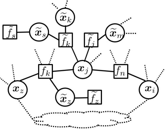
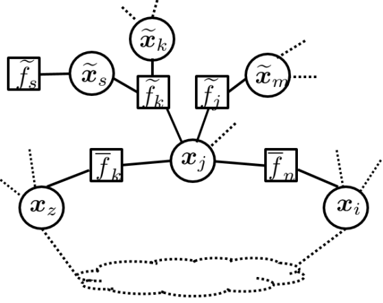
Figure 2: (a) An example of factor graph with a single loop and chains/trees topology, where the dashed line indicates possible chains/trees; (b) The equivalent factor graph of Fig 2 (a) with new factor functions that do not have neighboring variable nodes except those in the loop.

According to (11), computation of the messages in the first group does not depend on messages in the loop and is thus convergence guaranteed. Therefore, the message iteration number is replaced with a $\ast$ to denote the converged message. Also, from the definition of message computation in (11), if messages in the third group converge, the second group messages should also converge. Therefore, we next focus on showing the convergence of messages in the third group.

For a factor node $f_{k}$ in the loop with $\textbf{x}_{z}$ and $\textbf{x}_{j}$ being its two neighboring variable nodes in the loop and $\widetilde{\textbf{x}}_{z}$ being its neighboring variable node outside the loop, according to the definition of message computation in (12), we have

$$\begin{split}m^{\left(\ell\right)}_{f_{k}\to j}\left(\textbf{x}_{j}\right)&=\int\int f_{k}\times m^{\left(\ell\right)}_{z\to f_{k}}\left(\textbf{x}_{z}\right)\prod_{\widetilde{z}\in{\mathcal{B}}\left(f_{k}\right)\setminus j}m^{\ast}_{\widetilde{z}\to f_{k}}\left(\widetilde{\textbf{x}}_{z}\right)\,\mathrm{d}\left\{\widetilde{\textbf{x}}_{z}\right\}_{\widetilde{z}\in{\mathcal{B}}\left(f_{k}\right)\setminus j}\,\mathrm{d}\textbf{x}_{z},\\ &=\int m^{\left(\ell\right)}_{z\to f_{k}}\left(\textbf{x}_{z}\right)\left[\int f_{k}\times\prod_{\widetilde{z}\in{\mathcal{B}}\left(f_{k}\right)\setminus j}m^{\ast}_{\widetilde{z}\to f_{k}}\left(\widetilde{\textbf{x}}_{z}\right)\,\mathrm{d}\left\{\widetilde{\textbf{x}}_{z}\right\}_{\widetilde{z}\in{\mathcal{B}}\left(f_{k}\right)\setminus j}\right]\,\mathrm{d}\textbf{x}_{z}.\end{split}$$ (44)

As shown in Lemma 2, $m^{\ast}_{\widetilde{z}\to f_{k}}\left(\widetilde{\textbf{x}}_{z}\right)$ must be in Gaussian function form, which is denoted by $m^{\ast}_{\widetilde{z}\to f_{k}}\left(\widetilde{\textbf{x}}_{z}\right)\propto\mathcal{N}\left(\widetilde{\textbf{x}}_{z}|\textbf{v}_{\widetilde{z}\to f_{k}}^{\ast},\left[\textbf{J}_{\widetilde{z}\to f_{k}}^{\ast}\right]^{-1}\right)$. Besides, from (1) we obtain

$$f_{k}=\mathcal{N}\left(\textbf{y}_{k}|\textbf{A}_{k,z}{\textbf{x}}_{z}+\textbf{A}_{k,j}{\textbf{x}}_{j}+\sum_{\widetilde{z}\in\mathcal{B}\left(f_{k}\right)}\textbf{A}_{k,\widetilde{z}}\widetilde{\textbf{x}}_{z},\textbf{R}_{k}\right).$$

It can be shown that the inner integration in the second line of (44) is given by

$$\mathcal{N}\left(\overline{\textbf{y}}_{k}|\overline{\textbf{A}}_{k,z}\textbf{x}_{z}\\ +\overline{\textbf{A}}_{k,j}\textbf{x}_{j},\overline{\textbf{R}}_{k}\right)\triangleq\overline{f}_{k},$$

where the overbar is used to denote the new constant matrix or vector. Then (44) can be written as

$$\begin{split}m^{\left(\ell\right)}_{f_{k}\to j}\left(\textbf{x}_{j}\right)=\int\overline{f}_{k}\times m^{\left(\ell\right)}_{z\to f_{k}}\left(\textbf{x}_{z}\right)\,\mathrm{d}\textbf{x}_{z}.\end{split}$$ (45)

Comparing (45) with (12), we obtain $m^{\left(\ell\right)}_{f_{k}\to j}\left(\textbf{x}_{j}\right)$ as if $m^{\left(\ell\right)}_{\overline{f}_{k}\to j}\left(\textbf{x}_{j}\right)$ is being passed to a factor node $\overline{f}_{k}$. Therefore, a factor graph with a single loop and multiple trees/chains is equivalent to a single loop factor graph in which each factor node has no neighboring variable node outside the loop. As a result, the example of Fig. 2 (a) is equivalent to Fig. 2 (b). In the following, we focus on this equivalent topology for the convergence analysis.

Note that, for arbitrary variable node $j$ in the loop, there are two neighboring factor nodes in the loop. Further, using the notation for the equivalent topology, (42) is reduced to

$$\begin{split}\textbf{v}^{\left(\ell\right)}_{j\to\overline{f}_{n}}=&-\left[\textbf{J}^{\ast}_{j\to\overline{f}_{n}}\right]^{-1}\overline{\textbf{A}}_{k,j}^{T}\textbf{T}_{k,j}^{-1}\overline{\textbf{A}}_{k,z}\textbf{v}^{\left(\ell-1\right)}_{z\to\overline{f}_{k}}\\ &+\underbrace{\overline{\textbf{b}}_{j\to\overline{f}_{n}}-\sum_{\widetilde{f}_{k}\in{\mathcal{B}}\left(j\right)\setminus f_{n}}\sum_{\widetilde{s}\in{\mathcal{B}}\left(\widetilde{f}_{k}\right)\setminus j}\left[\textbf{J}^{\ast}_{j\to\overline{f}_{n}}\right]^{-1}\overline{\textbf{A}}_{k,j}^{T}\overline{\textbf{M}}_{k,j}^{-1}\overline{\textbf{A}}_{k,\widetilde{s}}\textbf{v}^{\ast}_{\widetilde{s}\to\widetilde{f}_{k}}}_{\triangleq\textbf{c}_{j\to\overline{f}_{n}}},\end{split}$$ (46)

where $\textbf{v}^{\ast}_{\widetilde{s}\to\widetilde{f}_{k}}$ is the converged mean vector on the chain/tree;

$$\overline{\textbf{b}}_{j\to\overline{f}_{n}}=\left[\textbf{J}^{\ast}_{j\to\overline{f}_{n}}\right]^{-1}\sum_{\overline{f}_{k}\in{\mathcal{B}}\left(j\right)\setminus\overline{f}_{n}}\overline{\textbf{A}}_{k,j}^{T}\overline{\textbf{M}}_{k,j}^{-1}\overline{\textbf{y}}_{k}$$

with $\overline{\textbf{M}}_{k,j}=\overline{\textbf{R}}_{k}+\sum_{\widetilde{s}\in{\mathcal{B}}\left(\widetilde{f}_{k}\right)\setminus j}\overline{\textbf{A}}_{k,\widetilde{s}}\left[\textbf{J}^{\ast}_{\widetilde{s}\to\widetilde{f}_{k}}\right]^{-1}\overline{\textbf{A}}_{k,\widetilde{s}}^{T}$, and

$$\textbf{T}_{k,j}=\overline{\textbf{R}}_{k}+\overline{\textbf{A}}_{k,z}\left[\textbf{J}^{\ast}_{z\to\overline{f}_{k}}\right]^{-1}\overline{\textbf{A}}_{k,z}^{T},$$ (47)

with $\textbf{x}_{z}$ and $\overline{f}_{k}$ in the loop where $\overline{f}_{k}\in\mathcal{B}\left(j\right)\setminus\overline{f}_{n}$ and $\textbf{x}_{z}\in\mathcal{B}\left(\overline{f}_{k}\right)\setminus j$. By multiplying $\left[\textbf{J}^{\ast}_{j\to\overline{f}_{n}}\right]^{1/2}$ on both sides of (46), and defining $\bm{\beta}_{j\to\overline{f}_{n}}^{\left(\ell\right)}=\left[\textbf{J}^{\ast}_{j\to\overline{f}_{n}}\right]^{1/2}\textbf{v}^{\left(\ell\right)}_{j\to\overline{f}_{n}}$, we have

$$\bm{\beta}^{\left(\ell\right)}_{j\to\overline{f}_{n}}=-\left[\textbf{J}^{\ast}_{j\to\overline{f}_{n}}\right]^{-1/2}\overline{\textbf{A}}_{k,j}^{T}\textbf{T}_{k,j}^{-1}\overline{\textbf{A}}_{k,z}\left[\textbf{J}^{\ast}_{z\to\overline{f}_{k}}\right]^{-1/2}\bm{\beta}^{\left(\ell-1\right)}_{z\to\overline{f}_{k}}+\left[\textbf{J}^{\ast}_{j\to\overline{f}_{n}}\right]^{1/2}\textbf{c}_{j\to\overline{f}_{n}},$$ (48)

Let $\bm{\beta}^{\left(\ell-1\right)}$ contain $\bm{\beta}^{\left(\ell-1\right)}_{z\to\overline{f}_{k}}$ for all $\textbf{x}_{z}$ with $z\in\mathcal{B}\left(\overline{f}_{k}\right)$ and $\overline{f}_{k}$ being in the loop, and the index is arranged first on $k$ and then on $z$. Then, the above equation is written in a compact form as

$$\bm{\beta}^{\left(\ell\right)}_{j\to\overline{f}_{n}}=-\textbf{Q}_{j\to\overline{f}_{n}}\bm{\beta}^{\left(\ell-1\right)}+\left[\textbf{J}^{\ast}_{j\to\overline{f}_{n}}\right]^{1/2}\textbf{c}_{j\to\overline{f}_{n}},$$ (49)

where $\textbf{Q}_{j\to\overline{f}_{n}}$ is a row block matrix with the only nonzero block

$$\left[\textbf{J}^{\ast}_{j\to\overline{f}_{n}}\right]^{-1/2}\overline{\textbf{A}}_{k,j}^{T}\textbf{T}_{k,j}^{-1}\overline{\textbf{A}}_{k,z}\left[\textbf{J}^{\ast}_{z\to\overline{f}_{k}}\right]^{-1/2}$$

located at the position corresponding to the position $\bm{\beta}_{z\to\overline{f}_{k}}^{\left(\ell\right)}$ in $\bm{\beta}^{\left(\ell\right)}$. Then let Q be a matrix that stacks $\textbf{Q}_{j\to\overline{f}_{n}}$ as its row, where $j$ and $\overline{f}_{n}$ are in the loop with $j\in\mathcal{B}\left(\overline{f}_{n}\right)$. Besides, let c be the vector containing the subvector $\left[\textbf{J}^{\ast}_{j\to\overline{f}_{n}}\right]^{1/2}\textbf{c}_{j\to\overline{f}_{n}}$ with the same order as $\textbf{Q}_{j\to\overline{f}_{n}}$ in Q. We have

$$\bm{\beta}^{\left(\ell\right)}=-\textbf{Q}\bm{\beta}^{\left(\ell-1\right)}+\textbf{c}.$$ (50)

Since Q is a square matrix, $\rho\left(\textbf{Q}\right)\leq\sqrt{\rho\left(\textbf{Q}\textbf{Q}^{T}\right)}$ and therefore $\rho\left(\textbf{Q}\textbf{Q}^{T}\right)<1$ is the sufficient condition for the convergence of $\bm{\beta}^{\left(\ell\right)}$. We next investigate the elements in $\textbf{Q}\textbf{Q}^{T}$.

Due to the single loop structure of the graph, every $\bm{\beta}_{j\to\overline{f}_{n}}^{\left(\ell\right)}$ in (48) would be dependent on a unique $\bm{\beta}_{z\to\overline{f}_{k}}^{\left(\ell\right)}$, where $\overline{f}_{k}\in\mathcal{B}\left(j\right)\setminus\overline{f}_{n}$ and $z\in\mathcal{{\mathcal{B}}}\left(\overline{f}_{k}\right)\setminus j$ (i.e., the message two hops backward along the loop in the factor graph). Thus, the position of the non-zero block in $\textbf{Q}_{j\to\overline{f}_{n}}$ will be different and non-overlapping for different combinations of ($j,\overline{f}_{n}$). As a result, there exists a column permutation matrix $\bm{\Xi}$ such that $\textbf{Q}\bm{\Xi}$ is a block diagonal matrix. Therefore, $\left(\textbf{Q}\bm{\Xi}\right)\left(\textbf{Q}\bm{\Xi}\right)^{T}=\textbf{Q}\textbf{Q}^{T}$ is also a diagonal matrix, and we can write

$$\textbf{Q}\textbf{Q}^{T}=\texttt{Bdiag}\left\{\textbf{Q}_{j\to\overline{f}_{n}}\textbf{Q}_{j\to\overline{f}_{n}}^{T}\right\}_{\textrm{$j\in\mathcal{B}\left(\overline{f}_{n}\right)$. }}$$

As a consequence, $\rho\left(\textbf{Q}\textbf{Q}^{T}\right)<1$ is equivalent to $\rho\left(\textbf{Q}_{j\to\overline{f}_{n}}\textbf{Q}_{j\to\overline{f}_{n}}^{T}\right)<1$ for all $j$ and $\overline{f}_{n}$ in the loop with $j\in\mathcal{B}\left(\overline{f}_{n}\right)$. Following the definition of $\textbf{Q}_{j\to\overline{f}_{n}}$ below (49), we obtain

$$\begin{split}\textbf{Q}_{j\to\overline{f}_{n}}\textbf{Q}_{j\to\overline{f}_{n}}^{T}=&\left[\textbf{J}^{\ast}_{j\to\overline{f}_{n}}\right]^{-1/2}\overline{\textbf{A}}_{k,j}^{T}\textbf{T}_{k,j}^{-1}\overline{\textbf{A}}_{k,z}\left[\textbf{J}^{\ast}_{z\to\overline{f}_{k}}\right]^{-1}\overline{\textbf{A}}_{k,z}^{T}\textbf{T}_{k,j}^{-1}\overline{\textbf{A}}_{k,j}\left[\textbf{J}^{\ast}_{j\to\overline{f}_{n}}\right]^{-1/2}\\ =&\left[\textbf{J}^{\ast}_{j\to\overline{f}_{n}}\right]^{-1/2}\overline{\textbf{A}}_{k,j}^{T}\textbf{T}_{k,j}^{-1}\left(\textbf{T}_{k,j}-\overline{\textbf{R}}_{k}\right)\textbf{T}_{k,j}^{-1}\overline{\textbf{A}}_{k,j}\left[\textbf{J}^{\ast}_{j\to\overline{f}_{n}}\right]^{-1/2},\end{split}$$ (51)

where the second equation follows from the definition of $\textbf{T}_{k,j}$ in (47). Besides, since $\overline{\textbf{R}}_{k}\succ\textbf{0}$, we have $\textbf{T}_{k,j}-\overline{\textbf{R}}_{k}\prec\textbf{T}_{k,j}$. Following P B.2 in Appendix B, and due to $\textbf{T}_{k,j}=\textbf{T}_{k,j}^{T}$, we have

$$\begin{split}\textbf{T}_{k,j}^{-1/2}\left(\textbf{T}_{k,j}-\overline{\textbf{R}}_{k}\right)\textbf{T}_{k,j}^{-1/2}\prec\textbf{I}.\end{split}$$ (52)

Applying P B.2 in Appendix B again to (52), and making use of (51), we obtain

$$\begin{split}\textbf{Q}_{j\to\overline{f}_{n}}\textbf{Q}_{j\to\overline{f}_{n}}^{T}&\prec\left[\textbf{J}^{\ast}_{j\to\overline{f}_{n}}\right]^{-1/2}\overline{\textbf{A}}_{k,j}^{T}\textbf{T}_{k,j}^{-1}\overline{\textbf{A}}_{k,j}\left[\textbf{J}^{\ast}_{j\to\overline{f}_{n}}\right]^{-1/2}.\end{split}$$ (53)

According to (47), we have

$$\overline{\textbf{A}}_{k,j}^{T}\textbf{T}_{k,j}^{-1}\overline{\textbf{A}}_{k,j}=\overline{\textbf{A}}_{k,j}^{T}\left[\overline{\textbf{R}}_{k}+\overline{\textbf{A}}_{k,z}\left[\textbf{J}^{\ast}_{z\to\overline{f}_{k}}\right]^{-1}\overline{\textbf{A}}_{k,z}^{T}\right]^{-1}\overline{\textbf{A}}_{k,j}.$$ (54)

On the other hand, using (19), due to $\mathcal{B}\left(\overline{f}_{k}\right)\setminus j=\textbf{x}_{z}$ in the considered topology, the right hand side of (54) is $\textbf{J}^{\ast}_{\overline{f}_{k}\to j}$. Therefore, (53) is further written as

$$\begin{split}\textbf{Q}_{j\to\overline{f}_{n}}\textbf{Q}_{j\to\overline{f}_{n}}^{T}&\prec\left[\textbf{J}^{\ast}_{j\to\overline{f}_{n}}\right]^{-1/2}\textbf{J}^{\ast}_{\overline{f}_{k}\to j}\left[\textbf{J}^{\ast}_{j\to\overline{f}_{n}}\right]^{-1/2}.\end{split}$$ (55)

From (16), $\textbf{J}^{\ast}_{j\to\overline{f}_{n}}=\textbf{W}_{j}^{-1}+\textbf{J}^{\ast}_{\overline{f}_{k}\to j}+\sum_{\widetilde{f}_{k}\in{\mathcal{B}}\left(j\right)\setminus\overline{f}_{n}}\textbf{J}_{\widetilde{f}_{k}\to j}^{\ast}$, thus $\textbf{J}^{\ast}_{\overline{f}_{k}\to j}\preceq\textbf{J}^{\ast}_{j\to\overline{f}_{n}}$. Therefore, $\left[\textbf{J}^{\ast}_{j\to\overline{f}_{n}}\right]^{-1/2}\textbf{J}^{\ast}_{\overline{f}_{k}\to j}\left[\textbf{J}^{\ast}_{j\to\overline{f}_{n}}\right]^{-1/2}\preceq\textbf{I}$, and, together with (55), we have

$$\textbf{Q}_{j\to\overline{f}_{n}}\textbf{Q}_{j\to\overline{f}_{n}}^{T}\prec\textbf{I}.$$

Hence $\rho\left(\textbf{Q}_{j\to\overline{f}_{n}}\textbf{Q}_{j\to\overline{f}_{n}}^{T}\right)<1$ for all $j$ and $\overline{f}_{n}$ in the loop and $j\in\mathcal{B}\left(\overline{f}_{n}\right)$, and equivalently $\rho\left(\textbf{Q}\right)<1$. This completes the proof.  

4.3 Convergence of Belief Covariance and Mean Vector

As the computation of the belief covariance $\textbf{P}_{i}^{\left(\ell\right)}$ depends on the message information matrix $\textbf{J}_{f_{n}\to i}^{\left(\ell\right)}$, using Theorems 6 and 11, we can derive the convergence and uniqueness properties of $\textbf{P}_{i}^{\left(\ell\right)}$.

Before we present the main result, we first present some properties of the part metric $\mathrm{d}\left(\textbf{X},\textbf{Y}\right)$, with positive definite arguments X, Y, and $\triangle\textbf{X}$. The proofs are provided in Appendix D.

Proposition 15

The part metric $\mathrm{d}\left(\textbf{X},\textbf{Y}\right)$ satisfies the following properties

P 15.1: $\mathrm{d}\left(\textbf{X}_{1}+\textbf{X}_{2},\textbf{Y}_{1}+\textbf{Y}_{2}\right)\leq\mathrm{d}\left(\textbf{X}_{1},\textbf{Y}_{1}\right)+\mathrm{d}\left(\textbf{X}_{2},\textbf{Y}_{2}\right)$;

P 15.2: $\mathrm{d}\left(\textbf{X},\textbf{Y}\right)=\mathrm{d}\left(\textbf{X}^{-1},\textbf{Y}^{-1}\right).$

We now have the following result.

Corollary 16

With arbitrary initial message information matrix $\textbf{J}^{\left(0\right)}_{f_{n}\to i}\succeq\textbf{0}$ for all $i\in\mathcal{V}$ and $f_{n}\in\mathcal{B}\left(i\right)$, the belief covariance matrix $\textbf{P}_{i}^{\left(\ell\right)}$ converges to a unique p.d. matrix at a doubly exponential rate with respect to any matrix norm before $\textbf{P}_{i}^{\left(\ell\right)}$ enters $\textbf{P}_{i}^{\ast}$’s neighborhood, which can be chosen to be arbitrarily small.

Proof  Since $\textbf{J}_{f_{n}\to i}^{\left(\ell\right)}$ converges to a p.d. matrix, and according to (23), $\textbf{P}_{i}^{\left(\ell\right)}$ also converges. Below, we study the convergence rate of $\textbf{P}_{i}^{\left(\ell\right)}$. According to the definition of $\textbf{P}_{i}^{(\ell)}$ in (23) and part metric in Definition 9, we have

$$\mathrm{d}\left([\textbf{P}_{i}^{\left(\ell\right)}]^{-1},[\textbf{P}_{i}^{\ast}]^{-1}\right)=\mathrm{d}\left(\textbf{W}_{i}^{-1}+\sum_{f_{n}\in{\mathcal{B}}\left(i\right)}\textbf{J}_{f_{n}\to i}^{\left(\ell\right)},\textbf{W}_{i}^{-1}+\sum_{f_{n}\in{\mathcal{B}}\left(i\right)}\textbf{J}_{f_{n}\to i}^{\ast}\right).$$

By applying P 15.1 to the above equation, we obtain

$$\mathrm{d}\left([\textbf{P}_{i}^{\left(\ell\right)}]^{-1},[\textbf{P}_{i}^{\ast}]^{-1}\right)\leq\mathrm{d}\left(\textbf{W}_{i}^{-1},\textbf{W}_{i}^{-1}\right)+\sum_{f_{n}\in{\mathcal{B}}\left(i\right)}\mathrm{d}\left(\textbf{J}_{f_{n}\to i}^{\left(\ell\right)},\textbf{J}_{f_{n}\to i}^{\ast}\right)=\sum_{f_{n}\in{\mathcal{B}}\left(i\right)}\mathrm{d}\left(\textbf{J}_{f_{n}\to i}^{\left(\ell\right)},\textbf{J}_{f_{n}\to i}^{\ast}\right).$$

According to (36), for all $i\in\mathcal{V}$ and $f_{n}\in\mathcal{B}(i)$, there exist a $c<1$ such that

$$\mathrm{d}\left(\textbf{J}_{f_{n}\to i}^{\left(\ell\right)},\textbf{J}_{f_{n}\to i}^{\ast}\right)<c^{\ell}\mathrm{d}\left(\textbf{J}_{f_{n}\to i}^{\left(0\right)},\textbf{J}_{f_{n}\to i}^{\ast}\right).$$

Applying the above inequality to compute $\left[\textbf{P}_{i}^{(\ell)}\right]^{-1}$ in (24), we obtain

$$\mathrm{d}\left([\textbf{P}_{i}^{\left(\ell\right)}]^{-1},[\textbf{P}_{i}^{\ast}]^{-1}\right)<c^{\ell}\sum_{f_{n}\in{\mathcal{B}}\left(i\right)}\mathrm{d}\left(\textbf{J}_{f_{n}\to i}^{\left(0\right)},\textbf{J}_{f_{n}\to i}^{\ast}\right).$$

Following P 15.2, the above inequality is equivalent to

$$\mathrm{d}\left(\textbf{P}_{i}^{\left(\ell\right)},\textbf{P}_{i}^{\ast}\right)<c^{\ell}\sum_{f_{n}\in{\mathcal{B}}\left(i\right)}\mathrm{d}\left(\textbf{J}_{f_{n}\to i}^{\left(0\right)},\textbf{J}_{f_{n}\to i}^{\ast}\right),$$

where $\sum_{f_{n}\in{\mathcal{B}}\left(i\right)}\mathrm{d}\left(\textbf{J}_{f_{n}\to i}^{\left(0\right)},\textbf{J}_{f_{n}\to i}^{\ast}\right)$ is a constant. Following the same procedure as that from (36) to (38), we can prove that $\textbf{P}_{i}^{\left(\ell\right)}$ converges at a doubly exponential rate with respect to the monotone norm before $\textbf{P}_{i}^{\left(\ell\right)}$ enters $\textbf{P}_{i}^{\ast}$’s neighborhood, which can be chosen to be arbitrarily small.  

On the other hand, as shown in (24), the computation of the belief mean $\bm{\mu}_{i}^{\left(\ell\right)}$ depends on the belief covariance $\textbf{P}_{i}^{\left(\ell\right)}$ and the message mean $\textbf{v}^{\left(\ell\right)}_{f_{n}\to i}$. Thus, under the same condition as in Theorem 13, $\bm{\mu}^{\left(\ell\right)}_{i}$ is convergence guaranteed. Moreover, it is shown in (Weiss and Freeman, 2001b, Appendix) that, for Gaussian BP over a factor graph, the converged value of belief mean equals the optimal estimate in (3). Together with the convergence guaranteed topology revealed in Theorem 14, we have the following Corollary.

Corollary 17

With arbitrary $\textbf{J}_{f_{n}\to i}^{\left(0\right)}\succeq\textbf{0}$ and arbitrary $\textbf{v}^{\left(0\right)}_{f_{n}\to i}$ for all $i\in\mathcal{V}$ and $f_{n}\in\mathcal{B}\left(i\right)$, the mean vector $\bm{\mu}_{i}^{\left(\ell\right)}$ in (24) converges to the optimal estimate $\widehat{\textbf{x}}_{i}$ in (3) if and only if $\rho\left(\textbf{Q}\right)<1$, where Q is defined in (43). Furthermore, a sufficient condition to guarantee $\rho\left(\textbf{Q}\right)<1$ is when the factor graph contains only one single loop connected to multiple chains/trees.

5 Relationships with Existing Convergence Conditions

In this section, we show the relationship between our convergence condition for Gaussian BP and the recent proposed path-sum method (Giscard et al., 2016). We also show that our convergence condition is more general than the walk-summable condition (Malioutov et al., 2006) for the scalar case.

5.1 Relationship with the Path-sum Method

The path-sum method is proposed in (Giscard et al., 2012, 2013, 2016) to compute $\left(\textbf{W}^{-1}+\textbf{A}^{T}\textbf{R}^{-1}\textbf{A}\right)^{-1}$ in (3), in which the matrix inverse $\left(\textbf{W}^{-1}+\textbf{A}^{T}\textbf{R}^{-1}\textbf{A}\right)^{-1}$ is interpreted as the sum of simple paths and simple cycles on a weighted graph. The resulting formulation is guaranteed to converge to the correct value for any valid multivariate Gaussian distribution.

The BP message update equations (16), (17), (19), and (20) can be seen as a cut-off of path-sum by retaining only self-loops and backtracks (simple cycles of lengths one and two). In the presence of a graph with one or more loops, equations (16), (17), (19), and (20) do not include the terms related to simple cycles with length larger than $2$. This may be a potential cause for the possible divergence of the Gaussian BP algorithm. From this perspective, the divergence can be averted if none of the walks going around the loop(s) have weight greater than one, or equivalently, that the spectral radius of the block matrix representing the loop(s) is strictly less than one. This is an intuitive explanation of the condition $\rho(\textbf{Q})<1$ obtained in Theorem 13. It also immediately follows from these considerations that the convergence rate is at least geometric, with a cut-off of order $\ell$ yielding an $\mathcal{O}(\rho(\textbf{Q})^{\ell})$ error.

While the path-sum framework provides an insightful interpretation of the results obtained in this paper, the path-sum algorithm may not be efficiently implementable in distributed and parallel settings, as it requires the summation over all the paths of any length. In contrast, Gaussian BP, while paying the price of non-convergence in general loopy models, makes it possible to realize parallel and fully distributed inference. In summary, though the path-sum method converges for arbitrary valid Gaussian models, it is difficult to be adapted to a distributed and parallel inference setup as the Gaussian BP method.

5.2 Relationship with the Walk-Summable Condition

We show next that, in the setup of linear Gaussian models, the condition $\rho(\textbf{Q})<1$ as in Corollary 17 encompasses the Gaussian MRF based walk-summable (Malioutov et al. (2006)) in terms of convergence. As all existing results on Gaussian BP convergence (Malioutov et al., 2006; Moallemi and Roy, 2009b) only apply to scalar variables, we restrict the following discussion to only the scalar case. In (Malioutov et al., 2006), the starting point for the convergence analysis for Gaussian MRF is a joint multivariate Gaussian distribution

$$q(\textbf{x})\propto\exp\Big{\{}-\frac{1}{2}{\textbf{x}}^{T}\textbf{J}\textbf{x}+\textbf{h}^{T}\textbf{x}\Big{\}},$$ (56)

expressed in the normalized information form such that $\textbf{J}_{i,i}=1$ for all $i$. The underlying Gaussian distribution is factorized as (Malioutov et al. (2006))

$$q\left({\textbf{x}}\right)\propto\prod_{i\in\mathcal{V}}\psi_{i}\left(\textbf{x}_{i}\right)\prod_{J_{i,j}\neq 0;i\leq j}\psi_{i,j}\left(\textbf{x}_{i},\textbf{x}_{j}\right),$$ (57)

where

$$\psi_{i}\left(\textbf{x}_{i}\right)=\exp\left\{-\frac{1}{2}\textbf{J}_{i,i}\textbf{x}^{2}_{i}+\textbf{h}_{i}\right\}\quad\textrm{and}\quad\psi_{i,j}\left(\textbf{x}_{i},\textbf{x}_{j}\right)=\exp\left\{-\textbf{x}_{i}\textbf{J}_{i,j}\textbf{x}_{j}\right\}.$$

In Malioutov et al. (2006, Proposition 1), based on the interpretation that $\left[\textbf{J}^{-1}\right]_{i,j}$ is the sum of the weights of all the walks from variable $j$ to variable $i$ on the corresponding Gaussian MRF, a sufficient Gaussian BP convergence condition known as walk-summability is provided, which is equivalent to

$$\textbf{I}-|{\textbf{R}}|\succ\textbf{0},$$ (58)

together with the initial message variance inverse being set to $0$, where ${\textbf{R}}=\textbf{I}-{\textbf{J}}$ and $|\textbf{R}|$ is matrix of entrywise absolute values of R. In the following, we establish the relationship between walk-summable Gaussian MRF and linear Gaussian model by utilizing properties of H-matrices (Boman et al., 2005). We show that, with Gaussian MRF satisfying the walk-summable condition, the joint distribution $q(\textbf{x})$ in (57) can be reformulated as a special case of the linear Gaussian model based factorization in (10). Moreover, Gaussian BP on this particular linear Gaussian model always converges.

Definition 18

H-Matrices (Boman et al., 2005): A matrix X is an H-matrix if all eigenvalues of the matrix $\mathcal{H}(\textbf{X})$, where $[\mathcal{H}(\textbf{X})]_{i,i}=|\textbf{X}_{i,i}|$, and $[\mathcal{H}(\textbf{X})]_{i,j}=-|\textbf{X}_{i,j}|$ have positive real parts.

Proposition 19

Factor width at most $2$ factorization (Boman et al., 2005, Theorem 9): A symmetric H-matrix X that has non-negative diagonals can always be factorized as $\textbf{X}=\textbf{V}\textbf{V}^{T}$, where V is a real matrix with each column of V containing at most $2$ non-zeros.

Let $\omega$ be an arbitrary positive value that is smaller than the minimum eigenvalue of $\textbf{I}-|{\textbf{R}}|$ and also satisfies $0<\omega<1$. According to (58), we have $(1-\omega)\textbf{I}-|{\textbf{R}}|\succ\textbf{0}$. Furthermore, by applying $\mathcal{H}(\cdot)$ to $(1-\omega)\textbf{I}-{\textbf{R}}$, we have $[\mathcal{H}((1-\omega)\textbf{I}-{\textbf{R}})]_{i,i}=|(1-\omega)\textbf{I}-{\textbf{R}}|_{i,i}=1-\omega$ and $[\mathcal{H}((1-\omega)\textbf{I}-{\textbf{R}})]_{i,j}=-|[(1-\omega)\textbf{I}-{\textbf{R}})]_{i,j}|=-|{\textbf{R}}_{i,j}|$. Thus, $\mathcal{H}((1-\omega)\textbf{I}-{\textbf{R}})=(1-\omega)\textbf{I}-|{\textbf{R}}|\succ\textbf{0}$, and we conclude that $(1-\omega)\textbf{I}-{\textbf{R}}$ is an H-matrix. According to Proposition 19, $(1-\omega)\textbf{I}-{\textbf{R}}={\textbf{J}}-\omega\textbf{I}=\textbf{V}\textbf{V}^{T},$ where each column of V contains at most $2$ non-zeros. Now, we can rewrite the joint distribution in (57) as

$$\begin{split}q({\textbf{x}})&\propto\exp\left\{-\frac{1}{2}{\textbf{x}}^{T}\left({\textbf{J}}-\omega\textbf{I}\right){\textbf{x}}-\frac{1}{2}\omega{\textbf{x}}^{T}{\textbf{x}}+{\textbf{h}}^{T}{\textbf{x}}\right\}\\ &=\exp\left\{-\frac{1}{2}\left({\textbf{V}}^{T}{\textbf{x}}\right)^{T}\left({\textbf{V}}^{T}{\textbf{x}}\right)-\frac{1}{2}\left(\omega{\textbf{x}}^{T}{\textbf{x}}-2{\textbf{h}}^{T}{\textbf{x}}\right)\right\}\\ &\propto\exp\left\{-\frac{1}{2}\sum_{n=1}^{M}\left(V_{n,n_{i}}x_{n_{i}}+V_{n,n_{j}}x_{n_{j}}\right)^{2}-\frac{1}{2}\sum_{n=1}^{M}\omega(x_{n}-\frac{h_{n}}{\omega})^{2}\right\},\end{split}$$ (59)

where $V_{n,n_{i}}$ and $V_{n,n_{j}}$ denote the two possible non-zero elements on the $n$-th column and $n_{i}$-th and $n_{j}$-th rows, and $M$ is the dimension of x. Thus, a walk-summable Gaussian MRF in (56) (or equivalently (57)) can always be written as

$$q({\textbf{x}})\propto\prod_{n=1}^{M}\underbrace{\mathcal{N}(x_{n}|\frac{1}{\omega}h_{n},\frac{1}{\omega})}_{p(x_{n})}\prod_{n=1}^{M}\underbrace{\mathcal{N}(0|V_{n,n_{i}}x_{n_{i}}+V_{n,n_{j}}x_{n_{j}},1)}_{f_{n}}.$$ (60)

Note that, in the above equation, $p(x_{n})$ serves as the prior distribution for $x_{n}$ as that in (10) and $f_{n}$ is the local likelihood function with local observation being $y_{n}=0$ and noise distribution $z_{n}\sim\mathcal{N}(z_{n}|0,1)$. Thus the above equation is a special case of the linear Gaussian model based factorization in (10) with the local likelihood function $f_{n}$ containing only a pair of variables. For this pairwise linear Gaussian model with scalar variables, it is shown in (Moallemi and Roy, 2009b) that $\rho(\textbf{Q})<1$ is fulfilled. Thus by Corollary 17, Gaussian BP always converges. In summary, for the factorization based on Gaussian MRF, if the walk-summable convergence condition is fulfilled, there is an equivalent joint distribution factorization based on linear Gaussian model; and Gaussian BP is convergence guaranteed for this linear Gaussian model.

In the following, we further demonstrate through an example that there exist Gaussian MRFs, in which the information matrix J fails to satisfy the walk-summable condition, but a convergence guaranteed Gaussian BP update based on the distributed linear Gaussian model representation can still be obtained. More specifically, consider the following information matrix J in a Gaussian MRF:

$$\textbf{J}=\left[\begin{matrix}\begin{smallmatrix}1&\frac{1}{3\sqrt{2}}&\frac{1}{\sqrt{3}}&\frac{\sqrt{2}}{3}\\ \frac{1}{3\sqrt{2}}&1&0&\frac{1}{3}\\ \frac{1}{\sqrt{3}}&0&1&\frac{1}{\sqrt{6}}\\ \frac{\sqrt{2}}{3}&\frac{1}{3}&\frac{1}{\sqrt{6}}&1\end{smallmatrix}\end{matrix}\right].$$ (61)

The eigenvalues of $\textbf{I}-|\textbf{R}|$ to $4$ decimal places are $-0.0754$, $0.9712$, $1.4780$, and $1.6262$. According to the walk-summable definition in (58), it is non walk-summable and the convergence condition in (Malioutov et al., 2006) is inconclusive as to whether Gaussian BP converges. On the other hand, we can study the Gaussian BP convergence of this example by employing a linear Gaussian model representation, and rewriting J as $\textbf{J}=\textbf{A}^{T}\textbf{R}^{-1}\textbf{A}+\textbf{W}^{-1}$, where

$$\textbf{A}=\left[\begin{matrix}\frac{2}{\sqrt{6}}&0&\frac{1}{\sqrt{2}}&\frac{1}{\sqrt{3}}\\ \frac{{1}}{\sqrt{6}}&\frac{{1}}{\sqrt{3}}&0&0\\ 0&\frac{{1}}{\sqrt{3}}&0&\frac{{1}}{\sqrt{3}}\end{matrix}\right],\quad\textbf{W}=\left[\begin{matrix}6&0&0&0\\ 0&3&0&0\\ 0&0&2&0\\ 0&0&0&3\end{matrix}\right],$$

and $\textbf{R}=\textbf{I}$. In Fig. 3, the joint distribution of this example with Gaussian MRF and the corresponding linear Gaussian model are represented by factor graphs. As it is shown in Corollary 17, for a factor graph that is the union of a forest and a single loop, as in Fig. 3(b), Gaussian BP always converges to the exact value. This is in sharp contrast to the inconclusive convergence property when the same joint distribution is expressed using the classical Gaussian MRF in (4).

In summary, we have shown that the linear Gaussian model with $\rho(\textbf{Q})<1$ encompasses walk-summable Gaussian MRF. Further, it is shown in (Malioutov et al., 2006) that the diagonally dominant convergence condition in (Weiss and Freeman, 2001a) for Gaussian BP is a special case of the walk-summable condition. Also, the convergence condition in (Su and Wu, 2015) is encompassed by walk-summable condition. Therefore, we have the Venn diagram in Fig. 4 summarizing the relations (in terms of convergence guarantees) between the convergence condition proposed in this paper and existing conditions.

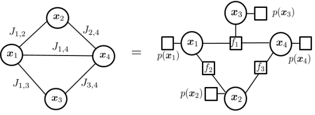
Figure 3: The Gaussian MRF corresponding to J in (61) with the factorization following (4); (b) The factor graph corresponding to J in (61) with the factorization following (10).

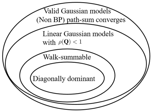
Figure 4: Venn diagram summarizing various subclasses of Gaussian models: the three inner most conditions are all for the BP algorithm while the path-sum in general does not constitute a BP algorithm.

6 Conclusions

This paper shows that, depending on how the factorization of the underlying joint Gaussian distribution is performed, Gaussian belief propagation (BP) may exhibit different convergence properties as different factorizations lead to fundamentally different recursive update structures. The paper studies the convergence of Gaussian BP derived from the factorization based on the distributed linear Gaussian model. We show that the condition we present for convergence of the marginal mean based on factorizations using the linear Gaussian model is more general than the walk-summable condition (Malioutov et al., 2006) (and references therein) that is based on the Gaussian Markov random field factorization. Further, the linear Gaussian model that is studied in this paper readily conforms to the physical network topology arising in large-scale networks.

Further, the paper analyzes the convergence of the Gaussian BP based distributed inference algorithm. In particular, we show analytically that, with arbitrary positive semidefinite matrix initialization, the message information matrix exchanged among agents converges to a unique positive definite matrix, and it approaches an arbitrarily small neighborhood of this unique positive definite matrix at a doubly exponential rate (with respect to any matrix norm). Regarding the initial information matrix, there exist positive definite initializations that guarantee faster convergence than the commonly used all-zero matrix. Moreover, under the positive semidefinite initial message information matrix condition, we present a necessary and sufficient condition of the belief mean vector to converge to the optimal centralized estimate. We also prove that Gaussian BP always converges if the corresponding factor graph is a union of a single loop and a forest. In particular, we show that the proposed convergence condition for Gaussian BP based on the linear Gaussian model leads to a strictly larger class of models in which Gaussian BP converges than those postulated by the Gaussian Markov random field based walk-summable condition. Finally, we discuss connections of Gaussian BP with the general path-sum algorithm. In the future, it will be interesting to explore if these path-sum interpretations can lead to modifications of the standard Gaussian BP algorithm that guarantee the convergence of Gaussian BP for larger classes of topologies while being also parallel and fully distributed.

Appendix A.

We first compute the first round updating message from variable node to factor node. Substituting $m^{\left(0\right)}_{f_{n}\to i}\left(\textbf{x}_{i}\right)\propto\exp\left\{-\frac{1}{2}||\textbf{x}_{j}-\textbf{v}^{\left(0\right)}_{f_{n}\to i}||^{2}_{\textbf{J}^{\left(0\right)}_{f_{n}\to i}}\right\}$ into (11) and, after algebraic manipulations, we obtain

$$m^{\left(1\right)}_{j\to f_{n}}\left(\textbf{x}_{j}\right)\propto\exp\left\{-\frac{1}{2}||\textbf{x}_{j}-\textbf{v}^{\left(1\right)}_{j\to f_{n}}||^{2}_{\textbf{J}^{\left(1\right)}_{j\to f_{n}}}\right\},$$ (62)

with

$$\textbf{J}^{\left(1\right)}_{j\to f_{n}}=\textbf{W}_{j}^{-1}+\sum_{f_{k}\in{\mathcal{B}}\left(j\right)\setminus f_{n}}\textbf{J}_{f_{k}\to j}^{\left(0\right)},$$

and

$$\textbf{v}^{\left(1\right)}_{j\to f_{n}}=\left[\textbf{J}^{\left(1\right)}_{j\to f_{n}}\right]^{-1}\left[\sum_{f_{k}\in{\mathcal{B}}\left(j\right)\setminus f_{n}}\textbf{J}_{f_{k}\to j}^{\left(0\right)}\textbf{v}^{\left(0\right)}_{f_{k}\to j}\right].$$

Next, we evaluate $m^{\left(1\right)}_{f_{n}\to i}\left(\textbf{x}_{i}\right)$. By substituting $m^{\left(1\right)}_{j\to f_{n}}\left(\textbf{x}_{j}\right)$ in (62) into (12), we obtain

$$\begin{split}m^{\left(1\right)}_{f_{n}\to i}\left(\textbf{x}_{i}\right)&\propto\int\ldots\int\exp\Big{\{}-\frac{1}{2}\big{(}\textbf{y}_{n}-\sum_{j\in\mathcal{B}\left(f_{n}\right)}\textbf{A}_{n,j}\textbf{x}_{j}\big{)}^{T}\textbf{R}^{-1}\big{(}\textbf{y}_{n}-\sum_{j\in\mathcal{B}\left(f_{n}\right)}\textbf{A}_{n,j}\textbf{x}_{j}\big{)}\Big{\}}\times\\ &\quad\quad\!\!\prod_{j\in{\mathcal{B}}\left(f_{n}\right)\setminus i}\exp\Big{\{}-\frac{1}{2}||\textbf{x}_{j}-\textbf{v}^{\left(1\right)}_{j\to f_{n}}||^{2}_{\textbf{J}^{\left(1\right)}_{j\to f_{n}}}\Big{\}}\,\mathrm{d}\{\textbf{x}_{j}\}_{j\in{\mathcal{B}}\left(f_{n}\right)\setminus i}.\end{split}$$ (63)

Let $\textbf{x}_{\left\{{\mathcal{B}}\left(f_{n}\right)\setminus i\right\}}$ and $\textbf{v}_{\left\{{\mathcal{B}}\left(f_{n}\right)\setminus i\right\}\to f_{n}}^{\left(1\right)}$ be stacked vectors containing $\textbf{x}_{j}$ and $\textbf{v}^{\left(1\right)}_{j\to f_{n}}$ as vector elements for all $j\in{\mathcal{B}}\left(f_{n}\right)\setminus i$ arranged in ascending order on $j$, respectively; $\textbf{A}_{n,\left\{{\mathcal{B}}\left(f_{n}\right)\setminus i\right\}}$ denotes a row block matrix containing $\textbf{A}_{n,j}$ as row elements for all $j\in{\mathcal{B}}\left(f_{n}\right)\setminus i$ arranged in ascending order; and $\textbf{J}^{\left(1\right)}_{\left\{{\mathcal{B}}\left(f_{n}\right)\setminus i\right\}\to f_{n}}$ is a block diagonal matrix with $\textbf{J}^{\left(1\right)}_{j\to f_{n}}$ as its block diagonal elements for all $j\in{\mathcal{B}}\left(f_{n}\right)\setminus i$ arranged in ascending order. Then, (63) can be reformulated as

$$m^{(1)}_{f_{n}\to i}(\textbf{x}_{i})\!\!\! \propto \!\!\!\!\int\ldots\int\exp\left\{-\frac{1}{2}||\textbf{y}_{n}-\textbf{A}_{n,i}\textbf{x}_{i}-\textbf{A}_{n,\{{\mathcal{B}}(f_{n})\setminus i\}}\textbf{x}_{\{{\mathcal{B}}(f_{n})\setminus i\}}^{T}||^{2}_{\textbf{R}^{-1}}\right\}$$ (64)

$$\quad\times\exp\left\{-\frac{1}{2}||\textbf{x}_{\{{\mathcal{B}}(f_{n})\setminus i\}}-\textbf{v}_{\{{\mathcal{B}}(f_{n})\setminus i\}\to f_{n}}^{(1)})||^{2}_{\widetilde{\textbf{J}}^{(1)}_{\{{\mathcal{B}}(f_{n})\setminus i\}\to f_{n}}}\right\}\mathrm{d}\textbf{x}_{\{{\mathcal{B}}(f_{n})\setminus i\}}$$

$$\propto \exp\left\{-\frac{1}{2}||\textbf{y}_{n}-\textbf{A}_{n,i}\textbf{x}_{i}||^{2}_{\textbf{R}^{-1}}\right\}$$

$$\times\int\ldots\int\exp\left\{\!-\!\frac{1}{2}(\textbf{x}_{\{{\mathcal{B}}(f_{n})\setminus i\}}^{T}\textbf{K}^{(1)}_{f_{n}\to i}\textbf{x}_{\{{\mathcal{B}}(f_{n})\setminus i\}}\!\!-\!2[\textbf{h}^{(1)}_{f_{n}\to i}]^{T}\textbf{x}_{\{{\mathcal{B}}(f_{n})\setminus i\}})\!\!\right\}\!\!\mathrm{d}\textbf{x}_{\{{\mathcal{B}}(f_{n})\setminus i\}},$$

where

$$\textbf{K}^{\left(1\right)}_{f_{n}\to i}=\textbf{A}_{n,\left\{{\mathcal{B}}\left(f_{n}\right)\setminus i\right\}}^{T}\textbf{R}^{-1}\textbf{A}_{n,\left\{{\mathcal{B}}\left(f_{n}\right)\setminus i\right\}}+\textbf{J}^{\left(1\right)}_{\left\{{\mathcal{B}}\left(f_{n}\right)\setminus i\right\}\to f_{n}}$$

and

$$\textbf{h}^{\left(1\right)}_{f_{n}\to i}=\textbf{A}_{n,\left\{{\mathcal{B}}\left(f_{n}\right)\setminus i\right\}}^{T}\textbf{R}^{-1}\left(\textbf{y}_{n}-\textbf{A}_{n,i}\textbf{x}_{i}\right)+\textbf{J}^{\left(1\right)}_{\left\{{\mathcal{B}}\left(f_{n}\right)\setminus i\right\}\to f_{n}}\textbf{v}_{\left\{{\mathcal{B}}\left(f_{n}\right)\setminus i\right\}\to f_{n}}^{\left(1\right)}.$$

By completing the square for the integrand of (64), we obtain

$$m^{\left(1\right)}_{f_{n}\to i}\left(\textbf{x}_{i}\right)\!\!\! \propto\!\!\! \alpha_{f_{n}\to i}^{\left(1\right)}\exp\left\{-\frac{1}{2}||\textbf{y}_{n}-\textbf{A}_{n,i}\textbf{x}_{i}||^{2}_{\textbf{R}_{n}^{-1}}+\frac{1}{2}\left[\textbf{h}^{\left(1\right)}_{f_{n}\to i}\right]^{T}\left[\textbf{K}^{\left(1\right)}_{f_{n}\to i}\right]^{-1}\textbf{h}^{\left(\ell\right)}_{f_{n}\to i}\right\},$$ (65)

with

$$\alpha_{f_{n}\to i}^{\left(1\right)}=\int\ldots\int\exp\left\{-\frac{1}{2}||\textbf{x}_{\left\{{\mathcal{B}}\left(f_{n}\right)\setminus i\right\}}-\left[\textbf{K}^{\left(1\right)}_{f_{n}\to i}\right]^{-1}\textbf{h}^{\left(1\right)}_{f_{n}\to i}||^{2}_{\textbf{K}^{\left(1\right)}_{f_{n}\to i}}\right\}\mathrm{d}\textbf{x}_{\left\{{\mathcal{B}}\left(f_{n}\right)\setminus i\right\}}.$$

Next, by applying the spectral theorem to $\textbf{K}^{\left(1\right)}_{f_{n}\to i}$ and after some algebraic manipulations, we simplify (65) as

$$m^{\left(1\right)}_{f_{n}\to i}\left(\textbf{x}_{i}\right)\propto\alpha_{f_{n}\to i}^{\left(1\right)}\exp\left\{-\frac{1}{2}||\textbf{x}_{i}-\textbf{v}^{\left(1\right)}_{f_{n}\to i}||_{\textbf{J}^{\left(1\right)}_{f_{n}\to i}}\right\},$$

with the inverse of the covariance, the information matrix

$$\begin{split}\textbf{J}^{\left(1\right)}_{f_{n}\to i}&=\textbf{A}_{n,i}^{T}\left[\textbf{R}_{n}+\sum_{j\in{\mathcal{B}}\left(f_{n}\right)\setminus i}\textbf{A}_{n,j}\left[\textbf{J}^{\left(1\right)}_{j\to f_{n}}\right]^{-1}\textbf{A}_{n,j}^{T}\right]^{-1}\textbf{A}_{n,i},\end{split}$$

and the mean vector

$$\begin{split}\textbf{v}^{\left(1\right)}_{f_{n}\to i}=\left[\textbf{J}_{f_{n}\to i}^{\left(1\right)}\right]^{-1}\textbf{A}_{n,i}^{H}\left[\textbf{R}_{n}+\sum_{j\in{\mathcal{B}}\left(f_{n}\right)\setminus i}\textbf{A}_{n,j}\left[\textbf{J}^{\left(1\right)}_{j\to f_{n}}\right]^{-1}\textbf{A}_{n,j}^{T}\right]^{-1}\left(\textbf{y}_{n}-\sum_{j\in{\mathcal{B}}\left(f_{n}\right)\setminus i}\textbf{A}_{n,j}\textbf{v}^{\left(1\right)}_{j\to f_{n}}\right),\end{split}$$

and

$$\alpha_{f_{n}\to i}^{\left(1\right)}\propto\int\ldots\int\exp\big{\{}-\frac{1}{2}\textbf{z}^{T}\bm{\Lambda}_{f_{n}\to i}^{\left(1\right)}\textbf{z}\big{\}}\,\mathrm{d}\textbf{z},$$ (66)

where $\bm{\Lambda}_{f_{n}\to i}^{\left(1\right)}$ is a diagonal matrix containing the eigenvalues of $\textbf{A}_{n,\left\{{\mathcal{B}}\left(f_{n}\right)\setminus i\right\}}^{T}\textbf{R}_{n}^{-1}\textbf{A}_{n,\left\{{\mathcal{B}}\left(f_{n}\right)\setminus i\right\}}+\textbf{J}^{\left(1\right)}_{\left\{{\mathcal{B}}\left(f_{n}\right)\setminus i\right\}\to f_{n}}$.

By induction, and following similar derivations as in (62) to (66), we obtain the general updating expressions as in (15) to (21).

Appendix B.

Before going into the proof of Lemma 2, we note the following properties of positive definite (p.d.) matrices. If $\textbf{X}\succ\textbf{0}$, $\textbf{Y}\succ\textbf{0}$, $\textbf{Z}\succeq\textbf{0}$ are of the same dimension, then we have (Du and Wu, 2013a):

P B.1: $\textbf{X}+\textbf{Y}\succ\textbf{0}$ and $\textbf{X}+\textbf{Z}\succ\textbf{0}$.

P B.2: $\textbf{A}^{T}\textbf{X}\textbf{A}\succ\textbf{0}$, $\textbf{A}^{T}\textbf{Z}\textbf{A}\succeq\textbf{0}$, $\textbf{A}\textbf{X}\textbf{A}^{T}\succeq\textbf{0}$ and $\textbf{A}\textbf{Z}\textbf{A}^{T}\succeq\textbf{0}$ for any full column rank matrix A with compatible dimension.

Now, we prove Lemma 2. If $\textbf{J}_{f_{k}\to j}^{\left(\ell-1\right)}\succeq\textbf{0}$ for all $f_{k}\in{\mathcal{B}}\left(j\right)\setminus f_{n}$, according to P B.1, $\sum_{f_{k}\in{\mathcal{B}}\left(j\right)\setminus f_{n}}\textbf{J}_{f_{k}\to j}^{\left(\ell-1\right)}\succeq\textbf{0}$. As $\textbf{W}_{j}^{-1}\succ\textbf{0}$, we have $\textbf{W}_{j}^{-1}+\sum_{f_{k}\in{\mathcal{B}}\left(j\right)\setminus f_{n}}\textbf{J}_{f_{k}\to j}^{\left(\ell-1\right)}\succ\textbf{0}$, which, according to (16), is equivalent to $\textbf{J}^{\left(\ell\right)}_{j\to f_{n}}\succ\textbf{0}$. Besides, as $\textbf{A}_{n,j}$ is full column rank, if $\left[\textbf{J}^{\left(\ell\right)}_{j\to f_{n}}\right]^{-1}\succ\textbf{0}$ for all $j\in{\mathcal{B}}\left(f_{n}\right)\setminus i$, according to P B.2, $\textbf{A}_{n,j}\left[\textbf{J}^{\left(\ell\right)}_{j\to f_{n}}\right]^{-1}\textbf{A}_{n,j}^{T}\succeq\textbf{0}$. With $\textbf{R}_{n}\succ\textbf{0}$, following P B.1, we have $\left[\textbf{R}_{n}+\sum_{j\in{\mathcal{B}}\left(f_{n}\right)\setminus i}\textbf{A}_{n,j}\left[\textbf{J}^{\left(\ell\right)}_{j\to f_{n}}\right]^{-1}\textbf{A}_{n,j}^{T}\right]^{-1}\succ\textbf{0}$. As $\textbf{A}_{n,i}$ is of full column rank, by applying P B.2 again, we have $\textbf{A}_{n,i}^{T}\left[\textbf{R}_{n}+\sum_{j\in{\mathcal{B}}\left(f_{n}\right)\setminus i}\textbf{A}_{n,j}\left[\textbf{J}^{\left(\ell\right)}_{j\to f_{n}}\right]^{-1}\textbf{A}_{n,j}^{T}\right]^{-1}\textbf{A}_{n,i}\succ\textbf{0}$, which according to (19) is equivalent to $\textbf{J}^{\left(\ell\right)}_{f_{n}\to i}\succ\textbf{0}$.

In summary, we have proved that 1) if $\textbf{J}_{f_{k}\to j}^{\left(\ell-1\right)}\succeq\textbf{0}$ for all $f_{k}\in{\mathcal{B}}\left(j\right)\setminus f_{n}$, then $\textbf{J}^{\left(\ell\right)}_{j\to f_{n}}\succ\textbf{0}$; 2) if $\left[\textbf{J}^{\left(\ell\right)}_{j\to f_{n}}\right]^{-1}\succ\textbf{0}$ for all $j\in{\mathcal{B}}\left(f_{n}\right)\setminus i$, then $\textbf{J}^{\left(\ell\right)}_{f_{n}\to i}\succ\textbf{0}$. Therefore, by setting $\textbf{J}_{f_{k}\to j}^{\left(0\right)}\succeq\textbf{0}$ for all $k\in\mathcal{V}$ and $j\in\mathcal{B}\left(f_{k}\right)$, according to the results of the first case, we have $\textbf{J}_{j\to f_{n}}^{\left(1\right)}\succ\textbf{0}$ for all $j\in\mathcal{V}$ and $f_{n}\in\mathcal{B}\left(j\right)$. Then, applying the second case, we further have $\textbf{J}_{f_{n}\to i}^{\left(1\right)}\succ\textbf{0}$ for all $n\in\mathcal{V}$ and $i\in\mathcal{B}\left(f_{n}\right)$. By repeatedly using the above arguments, it follows readily that $\textbf{J}_{f_{k}\to j}^{\left(\ell\right)}\succ\textbf{0}$ and $\textbf{J}_{j\to f_{n}}^{\left(\ell\right)}\succ\textbf{0}$ for $\ell\geq 1$ and with $j\in\mathcal{V}$, $f_{n},f_{k}\in\mathcal{B}\left(j\right)$. Furthermore, according to the discussion before Lemma 2, all messages $m^{\left(\ell\right)}_{j\to f_{n}}\left(\textbf{x}_{j}\right)$ and $m^{\left(\ell\right)}_{f_{n}\to i}\left(\textbf{x}_{i}\right)$ exist, and are in Gaussian form as in (15) and (18).

Appendix C.

First, Proposition 4, P 4.1 is proved. Suppose that ${\textbf{J}}^{\left(\ell\right)}\succeq{\textbf{J}}^{\left(\ell-1\right)}\succeq\textbf{0}$, i.e., $\textbf{J}_{f_{k}\to j}^{\left(\ell\right)}\succeq\textbf{J}_{f_{k}\to j}^{\left(\ell-1\right)}\succeq\textbf{0}$ for all ${\left(f_{k},j\right)\in\mathcal{\widetilde{B}}\left(f_{n},i\right)}$, we have

$$\textbf{W}_{j}^{-1}+\sum_{f_{k}\in{\mathcal{B}}\left(j\right)\setminus f_{n}}\textbf{J}_{f_{k}\to j}^{\left(\ell\right)}\succeq\textbf{W}_{j}^{-1}+\sum_{f_{k}\in{\mathcal{B}}\left(j\right)\setminus f_{n}}\textbf{J}_{f_{k}\to j}^{\left(\ell-1\right)}\succ\textbf{0}.$$

Then, according to the fact that if $\textbf{X}\succeq\textbf{Y}\succ\textbf{0}$, $\textbf{Y}^{-1}\succeq\textbf{X}^{-1}\succ\textbf{0}$, we have

$$\left[\textbf{W}_{j}^{-1}+\sum_{f_{k}\in{\mathcal{B}}\left(j\right)\setminus f_{n}}\textbf{J}_{f_{k}\to j}^{\left(\ell-1\right)}\right]^{-1}\succeq\left[\textbf{W}_{j}^{-1}+\sum_{f_{k}\in{\mathcal{B}}\left(j\right)\setminus f_{n}}\textbf{J}_{f_{k}\to j}^{\left(\ell\right)}\right]^{-1}\succ\textbf{0}.$$

Since $\textbf{A}_{n,j}$ is of full column rank and following P B.2 in Appendix B, we have

$$\textbf{A}_{n,j}\left[\textbf{W}_{j}^{-1}+\!\!\!\!\!\sum_{f_{k}\in{\mathcal{B}}\left(j\right)\setminus f_{n}}\!\textbf{J}_{f_{k}\to j}^{\left(\ell-1\right)}\right]^{-1}\!\!\!\!\textbf{A}_{n,j}^{T}\succeq\textbf{A}_{n,j}\left[\textbf{W}_{j}^{-1}+\!\!\!\!\!\sum_{f_{k}\in{\mathcal{B}}\left(j\right)\setminus f_{n}}\!\textbf{J}_{f_{k}\to j}^{\left(\ell\right)}\right]^{-1}\!\!\!\!\textbf{A}_{n,j}^{T}\succ\textbf{0}.$$

Following the same procedure of the proof above and due to $\textbf{R}\succ\textbf{0}$, we can further prove that

$$\begin{split}&\textbf{A}_{n,i}^{T}\left[\textbf{R}_{n}+\sum_{j\in{\mathcal{B}}\left(f_{n}\right)\setminus i}\textbf{A}_{n,j}\left[\textbf{W}_{j}^{-1}+\sum_{f_{k}\in{\mathcal{B}}\left(j\right)\setminus f_{n}}\textbf{J}_{f_{k}\to j}^{\left(\ell\right)}\right]^{-1}\textbf{A}_{n,j}^{T}\right]^{-1}\textbf{A}_{n,i}\\ \succeq&\textbf{A}_{n,i}^{T}\left[\textbf{R}_{n}+\sum_{j\in{\mathcal{B}}\left(f_{n}\right)\setminus i}\textbf{A}_{n,j}\left[\textbf{W}_{j}^{-1}+\sum_{f_{k}\in{\mathcal{B}}\left(j\right)\setminus f_{n}}\textbf{J}_{f_{k}\to j}^{\left(\ell-1\right)}\right]^{-1}\textbf{A}_{n,j}^{T}\right]^{-1}\textbf{A}_{n,i},\end{split}$$

which is equivalent to

$$\mathcal{F}_{n\to i}\left(\left\{\textbf{J}_{f_{k}\to j}^{\left(\ell\right)}\right\}_{\left(f_{k},j\right)\in\mathcal{\widetilde{B}}\left(f_{n},i\right)}\right)\succeq\mathcal{F}_{n\to i}\left(\left\{\textbf{J}_{f_{k}\to j}^{\left(\ell-1\right)}\right\}_{\left(f_{k},j\right)\in\mathcal{\widetilde{B}}\left(f_{n},i\right)}\right).$$

Since $\mathcal{F}$ contains $\mathcal{F}_{n\to i}\left(\cdot\right)$ as its component, Proposition 4, P 4.1 is proved.

Next, Proposition 4, P 4.2 is proved. Suppose that $\textbf{J}_{f_{k}\to j}^{\left(\ell\right)}\succ\textbf{0}$ for all ${\left(f_{k},j\right)\in\mathcal{\widetilde{B}}\left(f_{n},i\right)}$. As $\alpha>1$, we have

$$\alpha\textbf{W}_{j}^{-1}+\sum_{f_{k}\in{\mathcal{B}}\left(j\right)\setminus f_{n}}\alpha\textbf{J}_{f_{k}\to j}^{\left(\ell\right)}\succeq\textbf{W}_{j}^{-1}+\sum_{f_{k}\in{\mathcal{B}}\left(j\right)\setminus f_{n}}\alpha\textbf{J}_{f_{k}\to j}^{\left(\ell\right)}\succ\textbf{0},$$

where the equality holds when $\textbf{W}_{j}^{-1}=\textbf{0}$, which corresponds to non-informative prior for $\textbf{x}_{j}$. Applying the fact that if $\textbf{X}\succeq\textbf{Y}\succ\textbf{0}$, $\textbf{Y}^{-1}\succeq\textbf{X}^{-1}\succ\textbf{0}$, and, according to P B.2 in Appendix B, we obtain

$$\textbf{A}_{n,j}\left[\textbf{W}_{j}^{-1}+\!\!\!\!\!\!\sum_{f_{k}\in{\mathcal{B}}\left(j\right)\setminus f_{n}}\!\!\!\!\alpha\textbf{J}_{f_{k}\to j}^{\left(\ell\right)}\right]^{-1}\!\!\!\textbf{A}_{n,j}^{T}\succeq\textbf{A}_{n,j}\left[\alpha\textbf{W}_{j}^{-1}+\!\!\!\!\!\!\sum_{f_{k}\in{\mathcal{B}}\left(j\right)\setminus f_{n}}\!\!\!\!\alpha\textbf{J}_{f_{k}\to j}^{\left(\ell\right)}\right]^{-1}\!\!\!\textbf{A}_{n,j}^{T}\succeq\textbf{0}.$$

Since $\textbf{R}_{n}\succ\frac{1}{\alpha}\textbf{R}_{n}\succ\textbf{0}$, we have

$$\left[\frac{1}{\alpha}\textbf{R}_{n}+\!\!\!\sum_{j\in{\mathcal{B}}\left(f_{n}\right)\setminus i}\textbf{A}_{n,j}\left[\alpha\textbf{W}_{j}^{-1}+\sum_{f_{k}\in{\mathcal{B}}\left(j\right)\setminus f_{n}}\!\!\!\!\alpha\textbf{J}_{f_{k}\to j}^{\left(\ell\right)}\right]^{-1}\textbf{A}_{n,j}^{T}\right]^{-1}$$

$$\quad\succ\left[\textbf{R}_{n}+\!\!\!\sum_{j\in{\mathcal{B}}\left(f_{n}\right)\setminus i}\textbf{A}_{n,j}\left[\textbf{W}_{j}^{-1}+\sum_{f_{k}\in{\mathcal{B}}\left(j\right)\setminus f_{n}}\alpha\textbf{J}_{f_{k}\to j}^{\left(\ell\right)}\right]^{-1}\textbf{A}_{n,j}^{T}\right]^{-1}.$$

Finally, applying P B.2 in Appendix B to the above equation and taking out the common factor $\alpha$, we obtain

$$\alpha\textbf{A}_{n,i}^{T}\left[\textbf{R}_{n}+\sum_{j\in{\mathcal{B}}\left(f_{n}\right)\setminus i}\textbf{A}_{n,j}\left[\textbf{W}_{j}^{-1}+\sum_{f_{k}\in{\mathcal{B}}\left(j\right)\setminus f_{n}}\textbf{J}_{f_{k}\to j}^{\left(\ell\right)}\right]^{-1}\textbf{A}_{n,j}^{T}\right]^{-1}\textbf{A}_{n,i}$$

$$\succ\textbf{A}_{n,i}^{T}\left[\textbf{R}_{n}+\sum_{j\in{\mathcal{B}}\left(f_{n}\right)\setminus i}\textbf{A}_{n,j}\left[\textbf{W}_{j}^{-1}+\sum_{f_{k}\in{\mathcal{B}}\left(j\right)\setminus f_{n}}\alpha\textbf{J}_{f_{k}\to j}^{\left(\ell\right)}\right]^{-1}\textbf{A}_{n,j}^{T}\right]^{-1}\textbf{A}_{n,i}.$$

Therefore, $\alpha\mathcal{F}_{n\to i}\bigg{(}\left\{\textbf{J}_{f_{k}\to j}^{\left(\ell\right)}\right\}_{\left(f_{k},j\right)\in\mathcal{\widetilde{B}}\left(f_{n},i\right)}\bigg{)}\succ\mathcal{F}_{n\to i}\left(\left\{\alpha\textbf{J}_{f_{k}\to j}^{\left(\ell\right)}\right\}_{\left(f_{k},j\right)\in\mathcal{\widetilde{B}}\left(f_{n},i\right)}\right)$ if $\textbf{J}_{f_{k}\to j}^{\left(\ell\right)}\succ\textbf{0}$ for all ${\left(f_{k},j\right)\in\mathcal{\widetilde{B}}\left(f_{n},i\right)}$ and $\alpha>1$. As $\mathcal{F}$ contains $\mathcal{F}_{n\to i}\left(\cdot\right)$ as its component, Proposition 4, P 4.2 is proved. In the same way, we can prove $\mathcal{F}\left(\alpha^{-1}\textbf{J}^{\left(\ell\right)}\right)\succ\alpha^{-1}\mathcal{F}\left(\textbf{J}^{\left(\ell\right)}\right)$ if $\textbf{J}^{\left(\ell\right)}\succ\textbf{0}$ and $\alpha>1$.

At last, Proposition 4, P 4.3 is proved. From Lemma 2, if we have initial message information matrix $\textbf{J}^{\left(0\right)}_{f_{k}\to j}\succeq\textbf{0}$ for all $j\in\mathcal{V}$ and $f_{k}\in\mathcal{B}\left(j\right)$, then we have $\textbf{J}^{\left(\ell\right)}_{f_{k}\to j}\succ\textbf{0}$ for all $j\in\mathcal{V}$ and $f_{k}\in\mathcal{B}\left(j\right)$. In such case, obviously, $\textbf{J}^{\left(\ell\right)}\succeq\textbf{0}$. Applying $\mathcal{F}$ to both sides of this equation, and using Proposition 4, P 4.1, we have $\mathcal{F}\left(\textbf{J}^{\left(\ell\right)}\right)\succeq\mathcal{F}\left(\textbf{0}\right)$. On the other hand, using (27), it can be easily checked that $\mathcal{F}\left(\textbf{0}\right)=\textbf{A}^{T}\left[\bm{\Omega}+\textbf{H}\bm{\Psi}^{-1}\textbf{H}^{T}\right]^{-1}\textbf{A}\succ\textbf{0}$, where the inequality is from Lemma 2. For proving the upper bound, we start from the fact that

$$\sum_{j\in{\mathcal{B}}\left(f_{n}\right)\setminus i}\textbf{A}_{n,j}\left[\textbf{W}_{j}^{-1}+\sum_{f_{k}\in{\mathcal{B}}\left(j\right)\setminus f_{n}}\textbf{J}_{f_{k}\to j}^{\left(\ell-1\right)}\right]^{-1}\textbf{A}_{n,j}^{T}$$

in (25), and equivalently the corresponding term

$$\textbf{H}_{n,i}\left[\textbf{W}_{n,i}+\textbf{K}_{n,i}\left(\textbf{I}_{|\mathcal{B}\left(f_{n}\right)|-1}\otimes\textbf{J}^{\left(\ell-1\right)}\right)\textbf{K}_{n,i}^{T}\right]^{-1}\textbf{H}_{n,i}^{T}$$

in (26), are p.s.d. matrices. In (27), since

$$\textbf{H}\left[\bm{\Psi}+\textbf{K}\left(\mathbf{I}_{\sum_{n=1}^{M}|B\left(f_{n}\right)|\left(|B\left(f_{n}\right)|-1\right)}\otimes\textbf{J}^{\left(\ell-1\right)}\right)\textbf{K}^{T}\right]^{-1}\textbf{H}^{T}$$

contains $\textbf{H}_{n,i}\left[\textbf{W}_{n,i}+\textbf{K}_{n,i}\left(\textbf{I}_{|\mathcal{B}\left(f_{n}\right)|-1}\otimes\textbf{J}^{\left(\ell-1\right)}\right)\textbf{K}_{n,i}^{T}\right]^{-1}\textbf{H}_{n,i}^{T}$ as its block diagonal elements, it is also a p.s.d. matrix. With $\bm{\Omega}\succ\textbf{0}$, adding to the above result gives

$$\bm{\Omega}+\textbf{H}\left[\bm{\Psi}+\textbf{K}\left(\mathbf{I}_{\varphi}\otimes\textbf{J}^{\left(\ell\right)}\right)\textbf{K}^{T}\right]^{-1}\textbf{H}^{T}\succeq\bm{\Omega}\succ\textbf{0}.$$

Inverting both sides, we obtain $\bm{\Omega}^{-1}\succeq\left[\bm{\Omega}+\textbf{H}\left[\bm{\Psi}+\textbf{K}\left(\mathbf{I}_{\varphi}\otimes\textbf{J}^{\left(\ell\right)}\right)\textbf{K}^{T}\right]^{-1}\textbf{H}^{T}\right]^{-1}.$ Finally, applying P B.2 again gives

$$\textbf{A}^{T}\bm{\Omega}^{-1}\textbf{A}\succeq\textbf{A}^{T}\left[\bm{\Omega}+\textbf{H}\left[\bm{\Psi}+\textbf{K}\left(\mathbf{I}_{\varphi}\otimes\textbf{J}^{\left(\ell\right)}\right)\textbf{K}^{T}\right]^{-1}\textbf{H}^{T}\right]^{-1}\textbf{A}^{T}=\mathcal{F}\left(\textbf{J}^{\left(\ell\right)}\right).$$

Therefore, we have $\textbf{A}^{T}\bm{\Omega}^{-1}\textbf{A}\succeq\mathcal{F}\left(\textbf{J}^{\left(\ell\right)}\right)\succeq\textbf{A}^{T}\left[\bm{\Omega}+\textbf{H}\bm{\Psi}^{-1}\textbf{H}^{T}\right]^{-1}\textbf{A}\succ\textbf{0}$.

Appendix D.

Let $\mathrm{d}\left(\textbf{X}_{1},\textbf{Y}_{1}\right)=\exp\{a_{1}\}$ and $\mathrm{d}\left(\textbf{X}_{2},\textbf{Y}_{2}\right)=\exp\{a_{2}\}$, and $\mathrm{d}\left(\textbf{X}_{1}+\textbf{X}_{2},\textbf{Y}_{1}+\textbf{Y}_{2}\right)=\exp\{a_{3}\}$. First, P 15.1 is proved. According to the definition of part metric in Definition 9, for arbitrary symmetric p.d matrix $\textbf{X}_{1}$, $\textbf{X}_{2}$, $\textbf{Y}_{1}$, and $\textbf{Y}_{2}$, we have $\mathrm{d}\left(\textbf{X}_{1},\textbf{Y}_{1}\right)$, $\mathrm{d}\left(\textbf{X}_{2},\textbf{Y}_{2}\right)$, and $\mathrm{d}\left(\textbf{X}_{1}+\textbf{X}_{2},\textbf{Y}_{1}+\textbf{Y}_{2}\right)$ correspond to

$$a_{1}\textbf{X}_{1}\succeq\textbf{Y}_{1}\succeq\frac{1}{a_{1}}\textbf{X}_{1},\quad a_{2}\textbf{X}_{2}\succeq\textbf{Y}_{2}\succeq\frac{1}{a_{2}}\textbf{X}_{2},$$ (67)

$$a_{3}(\textbf{X}_{1}+\textbf{X}_{2})\succeq\textbf{Y}_{1}+\textbf{Y}_{2}\succeq\frac{1}{a_{3}}\left(\textbf{X}_{1}+\textbf{X}_{2}\right).$$ (68)

Since $\mathrm{d}\left(\textbf{X}_{1},\textbf{Y}_{1}\right)>0$ and $\mathrm{d}\left(\textbf{X}_{2},\textbf{Y}_{2}\right)>0$, we have $a_{1},a_{2}\geq 1$. And therefore $a_{1}+a_{2}>a_{1}$ and $a_{1}+a_{2}>a_{2}$. Then, according to (67), we have

$$(a_{1}+a_{2})\left(\textbf{X}_{1}+\textbf{X}_{2}\right)\succeq\textbf{Y}_{1}+\textbf{Y}_{2}\succeq\frac{1}{a_{1}+a_{2}}(\textbf{X}_{1}+\textbf{X}_{2}).$$ (69)

Following the definition of part matric, $a_{3}$ is the smallest value satisfy the inequality in (68). Thus, by comparing (69) with (68), we obtain $a_{1}+a_{2}\geq a_{3}$ Hence, $\mathrm{d}\left(\textbf{X}_{1}+\textbf{X}_{2},\textbf{Y}_{1}+\textbf{Y}_{2}\right)\leq\mathrm{d}\left(\textbf{X}_{1},\textbf{Y}_{1}\right)+\mathrm{d}\left(\textbf{X}_{2},\textbf{Y}_{2}\right)$.

Next, P 15.2 is proved. Following the part metric definition of $\mathrm{d}\left(\textbf{X}_{1},\textbf{Y}_{1}\right)$, $a_{1}\textbf{X}_{1}\succeq\textbf{Y}_{1}\succeq\frac{1}{a_{1}}\textbf{X}_{1}$, which is equivalent to $\textbf{Y}_{1}^{-1}\succeq\frac{1}{a_{1}}\textbf{X}_{1}^{-1}$ and ${a_{1}}\textbf{X}_{1}^{-1}\succeq\textbf{Y}_{1}^{-1}$. Thus, $\mathrm{d}\left(\textbf{X},\textbf{Y}\right)=\mathrm{d}\left(\textbf{X}^{-1},\textbf{Y}^{-1}\right).$

References

- Bickson and Malkhi (2008) D. Bickson and D. Malkhi. A unifying framework for rating users and data items in peer-to-peer and social networks. Peer-to-Peer Networking and Applications (PPNA) Journal, 1(2):93–103, 2008.
- Boman et al. (2005) E. G. Boman, D. Chen, O. Parekh, and S. Toledo. On factor width and symmetric H-matrices. Linear algebra and its applications, 405:239–248, 2005.
- Cattivelli and Sayed (2010) F. S. Cattivelli and A. H. Sayed. Diffusion LMS strategies for distributed estimation. IEEE Trans. Signal Processing, 58(3):1035–1048, 2010.
- Chertkov and Chernyak (2006) M. Chertkov and V. Y. Chernyak. Loop series for discrete statistical models on graphs. Journal of Statistical Mechanics: Theory and Experiment, 2006(06):P06009, 2006.
- Chueshov (2002) I. Chueshov. Monotone Random Systems Theory and Applications. New York: Springer, 2002.
- Ciarlet (1989) P. G. Ciarlet. Introduction to Numerical Linear Algebra and Optimisation. Cambridge University Press, 1989.
- Demmel (1997) J. W. Demmel. Applied Numerical Linear Algebra. SIAM, 1997.
- Du and Wu (2013a) J. Du and Y. C. Wu. Network-wide distributed carrier frequency offsets estimation and compensation via belief propagation. IEEE Trans. Signal Processing, 61(23):5868–5877, December 2013a.
- Du and Wu (2013b) J. Du and Y. C. Wu. Distributed clock skew and offset estimation in wireless sensor networks: Asynchronous algorithm and convergence analysis. IEEE Trans. Wireless Commun., 12(11):5908–5917, Nov 2013b.
- Du et al. (2017a) J. Du, S. Kar, and J. M. F. Moura. Distributed convergence verification for Gaussian belief propagation. In Asilomar Conference on Signals, Systems, and Computers, 2017a.
- Du et al. (2017b) J. Du, S. Ma, Y. C. Wu, S. Kar, and J. M. F. Moura. Convergence analysis of belief propagation for pairwise linear Gaussian models. In IEEE Global Conference on Signal and Information Processing, 2017b.
- Frey (1999) B. J. Frey. Local probability propagation for factor analysis. In Neural Information Processing Systems (NIPS), pages 442–448, December 1999.
- Giscard et al. (2012) P.-L. Giscard, S. Thwaite, and D. Jaksch. Walk-sums, continued fractions and unique factorisation on digraphs. arXiv preprint arXiv:1202.5523, 2012.
- Giscard et al. (2013) P.-L. Giscard, S. Thwaite, and D. Jaksch. Evaluating matrix functions by resummations on graphs: the method of path-sums. SIAM Journal on Matrix Analysis and Applications, 34(2):445–469, 2013.
- Giscard et al. (2016) P.-L. Giscard, Z. Choo, S. Thwaite, and D. Jaksch. Exact inference on Gaussian graphical models of arbitrary topology using path-sums. Journal of Machine Learning Research, 7(2):1–19, February 2016.
- Gómez et al. (2007) V. Gómez, J. M. Mooij, and H. J. Kappen. Truncating the loop series expansion for belief propagation. Journal of Machine Learning Research, 8:1987–2016, 2007.
- Hu et al. (2011) Y. Hu, A. Kuh, T. Yang, and A. Kavcic. A belief propagation based power distribution system state estimator. IEEE Comput. Intell. Mag., 2011.
- Ihler et al. (2005) A. T. Ihler, J. W. Fisher III, and A. S. Willsky. Loopy belief propagation: Convergence and effects of message errors. Journal of Machine Learning Research, 6:905–936, 2005.
- Kar (2010) S. Kar. Large Scale Networked Dynamical Systems: Distributed Inference. PhD thesis, Carnegie Mellon University, Pittsburgh, PA, Department of Electrical and Computer Engineering, June 2010.
- Kar and Moura (2013) S. Kar and J. M. F. Moura. Consensus + innovations distributed inference over networks: cooperation and sensing in networked systems. IEEE Signal Process. Mag., 30(3):99–109, 2013.
- Kar et al. (2013) S. Kar, J. M. F. Moura, and H.V. Poor. Distributed linear parameter estimation: asymptotically efficient adaptive strategies. SIAM Journal on Control and Optimization, 51(3):2200–2229, 2013.
- Krause and Nussbaum (1993) U. Krause and R. Nussbaum. A limit set trichotomy for self-mappings of normal cones in Banach spaces. Nonlinear Analysis, Theory, Methods & Applications, 20(7):855–870, 1993.
- Kschischang et al. (2001) F. R. Kschischang, B. J. Frey, and H.-A. Loeliger. Factor graphs and the sum-product algorithm. IEEE Trans. Information Theory, 47(2):498–519, February 2001.
- Lehmann (2012) F. Lehmann. Iterative mitigation of intercell interference in cellular networks based on Gaussian belief propagation. IEEE Trans. Veh. Technol., 61(6):2544–2558, July 2012.
- Malioutov et al. (2006) D. M. Malioutov, J. K. Johnson, and A. S. Willsky. Walk-sums and belief propagation in Gaussian graphical models. Journal of Machine Learning Research, 7(2):2031–2064, February 2006.
- Moallemi and Roy (2009a) C. C. Moallemi and B. Van Roy. Convergence of min-sum message passing for quadratic optimization. IEEE Trans. Information Theory, 55(5):2413–2423, 2009a.
- Moallemi and Roy (2009b) C. C. Moallemi and B. Van Roy. Convergence of min-sum message passing for quadratic optimization. IEEE Transactions on Information Theory, 55(5):2413–2423, 2009b.
- Mooij and Kappen (2005) J. M. Mooij and H. J. Kappen. Sufficient conditions for convergence of loopy belief propagation. In F. Bacchus and T. Jaakkola, editors, Proceedings of the 21st Annual Conference on Uncertainty in Artificial Intelligence (UAI-05), pages 396–403, Corvallis, Oregon, 2005. AUAI Press.
- Mooij and Kappen (2007) J. M. Mooij and H. J. Kappen. Sufficient conditions for convergence of the sum-product algorithm. IEEE Transactions on Information Theory, 53(12):4422–4437, December 2007.
- Murphy (2012) K. P. Murphy. Machine Learning: A Probabilistic Perspective. The MIT Press, 2012.
- Murphy et al. (1999) K. P. Murphy, Y. Weiss, and M. I. Jordan. Loopy belief propagation for approximate inference: an empirical study. In 15th Conf. Uncertainty in Artificial Intelligence (UAI), Stockholm, Sweden, pages 467–475, July 1999.
- National Research Council (2013) National Research Council. Frontiers in Massive Data Analysis. Washington, DC: The National Academies Press, 2013.
- Ng et al. (2008) B. L. Ng, J. S. Evans, S. V. Hanly, and D. Aktas. Distributed downlink beamforming with cooperative base stations. IEEE Trans. Information Theory, 54(12):5491–5499, December 2008.
- Noorshams and Wainwright (2013) N. Noorshams and M. J. Wainwright. Belief propagation for continuous state spaces: Stochastic message-passing with quantitative guarantees. Journal of Machine Learning Research, 14:2799–2835, 2013.
- Ravanbakhsh and Greiner (2015) S. Ravanbakhsh and R. Greiner. Perturbed message passing for constraint satisfaction problem. Journal of Machine Learning Research, 16:1249–1274, 2015.
- Shental et al. (2008a) O. Shental, P. H. Siegel, J. K. Wolf, D. Bickson, and D. Dolev. Gaussian belief propagation solver for systems of linear equations. In 2008 IEEE International Symposium on Information Theory (ISIT 2008), pages 1863–1867, July 2008a.
- Shental et al. (2008b) O. Shental, P. H. Siegel, J. K. Wolf, D. Bickson, and D. Dolev. Gaussian belief propagation solver for systems of linear equations. In 2008 IEEE International Symposium on Information Theory, pages 1863–1867, 2008b.
- Su and Wu (2015) Q. Su and Y. C. Wu. On convergence conditions of Gaussian belief propagation. IEEE Trans. Signal Processing, 63(5):1144–1155, March 2015.
- Tan and Li (2010) X. Tan and J. Li. Computationally efficient sparse Bayesian learning via belief propagation. IEEE Trans. Signal Processing, 58(4):2010–2021, April 2010.
- Weiss (2000) Y. Weiss. Correctness of local probability propagation in graphical models with loops. Neural Computation,, 12:1–41, 2000.
- Weiss and Freeman (2001a) Y. Weiss and W. T. Freeman. Correctness of belief propagation in Gaussian graphical models of arbitrary topology. Neural Computation, 13(10):2173–2200, March 2001a.
- Weiss and Freeman (2001b) Y. Weiss and W. T. Freeman. On the optimality of solutions of the max-product belief-propagation algorithm in arbitrary graphs. IEEE Trans. Information Theory, 47(2):736–744, February 2001b.
- Xiong et al. (2010) R. Xiong, W. Ding, S. Ma, and W. Gao. A practical algorithm for tanner graph based image interpolation. In 2010 IEEE International Conference on Image Processing (ICIP 2010), pages 1989–1992, 2010.
- Zeidler (1985) E. Zeidler. Nonlinear Analysis and its Applications IV-Applications to Mathematical Physics. Springer-Verlag New York Inc., 1985.
- Zhang et al. (2010) G. Zhang, W. Xu, and Y. Wang. Fast distributed rate control algorithm with QoS support in ad-hoc networks. In 2010 IEEE Global Telecommunications Conference (GLOBECOM 2010), pages 1–5, December 2010.