Large thermoelectric effect in ballistic Andreev interferometers

Abstract

Employing quasiclassical theory of superconductivity combined with Keldysh technique we investigate large thermoelectric effect in multiterminal ballistic normal-superconducting (NS) hybrid structures. We argue that this effect is caused by electron-hole asymmetry generated by coherent Andreev reflection of quasiparticles at interfaces of two different superconductors with non-zero phase difference. Within our model we derive a general expression for thermoelectric voltages $V_{T1,2}$ induced in two different normal terminals exposed to a thermal gradient. Our results apply at any temperature difference in the subgap regime and allow to explicitly analyze both temperature and phase dependencies of $V_{T1,2}$ demonstrating that in general there exists no fundamental relation between these voltages and the equilibrium Josephson current in SNS junctions.

I Introduction

Thermoelectric effect (i.e. the appearance of an electric current upon application of a thermal gradient) in superconductors remains an intriguing topic that attracts a lot of interest over last decades NL . While usually the magnitude of this effect in generic metals and superconductors remains small (being proportional to the ratio between temperature and the Fermi energy $T/\varepsilon_{F}$), it can increase by orders of magnitude provided electron-hole symmetry is lifted, e.g., due to spin-dependent scattering of electrons. This situation was predicted to occur in a variety of structures, such as superconductors doped with magnetic impurities Kalenkov12 , superconductor-ferromagnet hybrids with the density of states spin-split by the exchange and/or Zeeman fields Machon ; Ozaeta or superconductor-normal metal (SN) bilayers with spin-active interfaces KZ14 ; KZ15 . In accordance with theoretical predictions large thermoelectric currents were recently observed in superconductor-ferromagnet tunnel junctions in high magnetic fields Beckmann .

Large thermoelectric effect was also observed in multiterminal hybrid SNS structures with no magnetic inclusions Venkat1 ; Venkat2 ; Petrashov03 ; Venkat3 . Being exposed to a temperature gradient such structures (frequently called Andreev interferometers) were found to develop a thermopower signal which magnitude was not restricted by a small parameter $T/\varepsilon_{F}$ and, furthermore, turned out to be a periodic function of the superconducting phase difference $\chi$ across the corresponding SNS junction. The latter observation indicates that macroscopic quantum coherence can play an important role and poses a question about the relation between thermoelectric and Josephson effects in the systems under consideration. Subsequent theoretical analysis Seviour00 ; KPV ; VH ; VP indeed demonstrated that the thermoelectric effect in Andreev interferometers can be large and confirmed the periodic dependence of the thermopower on the phase difference $\chi$. At the same time, there appear to be no general consensus in the literature concerning the basic physical origin of this effect. While the authors KPV emphasized an important role of electron-hole imbalance, Virtanen and Heikkilä VH , on the contrary, proposed that in Andreev interferometers a non-vanishing thermopower signal can be generated even provided electron-hole symmetry is maintained and that the dominant part of this signal can be directly related to the difference between the equilibrium values for the Josephson current at temperatures $T_{1}$ and $T_{2}$. Subsequently, Volkov and Pavlovskii VP argued that in general no such simple relation between the thermopower and the Josephson current can be established and that under certain conditions the former can still remain large even though the latter gets strongly suppressed by temperature effects.

The existing theory Seviour00 ; KPV ; VH ; VP merely deals with the experimentally relevant diffusive limit in which case the analysis may become rather cumbersome forcing the authors either to employ numerics or to resort to various approximations. On the other hand, in order to clarify the physical origin of a large thermoelectric effect in Andreev interferometers one could take a different route focusing the analysis on the ballistic limit. A clear advantage of this approach is the possibility to employ the notion of semiclassical electron trajectories and in this way to treat the problem exactly. Below we will follow this route.

The structure of the paper is as follows. In Sec. II we define our model and describe the quasiclassical formalism which will be employed in our further analysis. In Sec. III we demonstrate that the quasiclassical Eilenberger equations supplemented by Zaitsev boundary conditions can be conveniently resolved with the aid of the so-called Riccati parameterization of the Green functions. Specific quasiparticle trajectories and their contributions to electric currents are identified in Sec. IV where we also discuss the conditions for electron-hole symmetry violation in our system. In Sec. V we evaluate the thermoelectric voltages induced by applying a temperature gradient and demonstrate that these voltages can be large because of the presence of electron-hole asymmetry in Andreev interferometers. Sec. VI is devoted to further analysis of the relation between thermoelectric and Josephson effects. Some technical details of our calculation are displayed in Appendix.

II The model and quasiclassical formalism

Let us consider an NSNSN structure shown in Fig. 1. Two superconductors with phase difference $\chi=\chi_{1}-\chi_{2}$ are connected to a normal wire. The two ends of this normal wire are maintained at temperatures $T_{1}$ and $T_{2}$ and voltages $V_{1}$ and $V_{2}$ respectively. Within our model we deliberately choose to disregard electron scattering on impurities and boundary imperfections, in which case electron motion is ballistic and can be conveniently described in terms of quasiclassical trajectories. In addition, we will disregard inelastic electron relaxation inside our system by assuming the inelastic relaxation length to exceed the system size. In this case inelastic electron relaxation can only occur deep inside normal terminals $\mathrm{N_{1}}$ and $\mathrm{N_{2}}$.

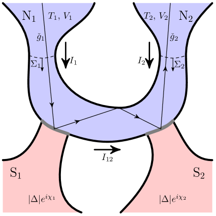
Figure 1: (Color online) Normal wire connected to normal and superconducting leads. Normal leads are maintained at temperatures $T_{1}$ and $T_{2}$ and voltages $V_{1}$ and $V_{2}$ respectively. An example of a quasiclassical electron trajectory relevant for the thermoelectric effect under consideration is also illustrated.

In what follows we will employ the quasiclassical theory of superconductivity based on the Eilenberger equations Eil ; bel . Under the above assumptions adopted within our model these equations take the form

$$\left[\hat{\Omega},\hat{g}^{R,A,K}\right]+i\bm{v}_{F}\nabla\hat{g}^{R,A,K}(\bm{p}_{F},\bm{r},\varepsilon)=0,\quad\check{g}^{2}=1,$$ (1)

where $\hat{g}^{R,A,K}$ are energy-integrated retarded, advanced and Keldysh $2\times 2$ matrix Green functions. The matrices $\hat{\Omega}$ and $\check{g}$ have the following structure

$$\hat{\Omega}=\begin{pmatrix}\varepsilon&\Delta\\ -\Delta^{*}&-\varepsilon\end{pmatrix},\quad\check{g}=\begin{pmatrix}\hat{g}^{R}&\hat{g}^{K}\\ 0&\hat{g}^{A}\end{pmatrix},$$ (2)

where $\Delta$ and $\varepsilon$ are respectively the superconducting order parameter and the quasiparticle energy. Electric current density can be expressed in terms of the Keldysh Green function in the standard manner as

$$\bm{j}(\bm{r})=-\dfrac{eN_{0}}{4}\int d\varepsilon\left<\bm{v}_{F}\operatorname{\mathrm{Sp}}[\hat{\tau}_{3}\hat{g}^{K}(\bm{p}_{F},\bm{r},\varepsilon)]\right>,$$ (3)

where $\bm{p}_{F}=m\bm{v}_{F}$ is the electron Fermi momentum vector, $\hat{\tau}_{3}$ is the Pauli matrix in the Nambu space and $N_{0}=mp_{F}/(2\pi^{2})$ is the normal density of states at the Fermi level. Here the angular brackets $\left<\cdots\right>$ denote averaging over the Fermi momentum directions.

III Riccati parameterization and boundary conditions

For the system under consideration the Eilenberger equations can be solved exactly. In order to proceed we restrict our analysis to quasiparticles propagating in the normal metal with subgap energies $|\varepsilon|<|\Delta|$ and employ the so-called Riccati parameterization for the retarded and advanced Green functions Schopohl95

$$\hat{g}^{R,A}=\pm\hat{N}^{R,A}\begin{pmatrix}1+\gamma^{R,A}\tilde{\gamma}^{R,A}&2\gamma^{R,A}\\ -2\tilde{\gamma}^{R,A}&-1-\tilde{\gamma}^{R,A}\gamma^{R,A}\\ \end{pmatrix},$$ (4)

where $\gamma^{R,A}$, $\tilde{\gamma}^{R,A}$ are Riccati amplitudes and

$$\hat{N}^{R,A}=\begin{pmatrix}(1-\gamma^{R,A}\tilde{\gamma}^{R,A})^{-1}&0\\ 0&(1-\tilde{\gamma}^{R,A}\gamma^{R,A})^{-1}\\ \end{pmatrix}.$$ (5)

Parameterization of the Keldysh Green function $\hat{g}^{K}$ also contains the two distribution functions $x$ and $\tilde{x}$. It reads Eschrig00

$$\hat{g}^{K}=2\hat{N}^{R}\begin{pmatrix}x-\gamma^{R}\tilde{x}\tilde{\gamma}^{A}&-\gamma^{R}\tilde{x}+x\gamma^{A}\\ -\tilde{\gamma}^{R}x+\tilde{x}\tilde{\gamma}^{A}&\tilde{x}-\tilde{\gamma}^{R}x\gamma^{A}\\ \end{pmatrix}\hat{N}^{A}.$$ (6)

In the normal metal (i.e. for $\Delta\equiv 0$) Riccati amplitudes $\gamma^{R,A}$, $\tilde{\gamma}^{R,A}$ and distribution functions $x$, $\tilde{x}$ obey the following simple equations

$$i\bm{v}_{F}\nabla\gamma^{R,A}=-2\varepsilon\gamma^{R,A},\quad i\bm{v}_{F}\nabla\tilde{\gamma}^{R,A}=2\varepsilon\tilde{\gamma}^{R,A},$$ (7)

$$i\bm{v}_{F}\nabla x=0,\quad i\bm{v}_{F}\nabla\tilde{x}=0.$$ (8)

Within the quasiclassical approximation adopted here quasiparticles propagate along the straight line trajectories between each two scattering events which can only occur at the boundaries of the normal metal wire. Of interest for us here is to describe quasiparticle scattering at the interfaces between the normal metal and each of the two superconductors. This task is accomplished in the standard manner with the aid of the Zaitsev boundary conditions Zaitsev84 for the quasiclassical Green functions rewritten in terms of the above Riccati amplitudes and the distribution functionsEschrig00 .

Consider, for instance, a quasiparticle propagating from the first normal terminal, being reflected at each of the two NS interfaces and leaving the system through the second normal terminal. The corresponding quasiparticle trajectory is indicated in Fig. 1. It is important to emphasize that here we only account for quasiparticles with subgap energies which cannot penetrate into superconductors suffering either normal or Andreev reflection at both NS interfaces. It is easy to verify that the distribution functions for such quasiparticles take the form

$$x=\left[1-\gamma^{R}\tilde{\gamma}^{A}\right]x_{1},\quad\tilde{x}=\left[1-\tilde{\gamma}^{R}\gamma^{A}\right]\tilde{x}_{2}$$ (9)

obeying both Eilenberger equations and the corresponding boundary conditions at NS interfaces. Here $\gamma^{R,A}$ and $\tilde{\gamma}^{R,A}$ are Riccati amplitudes along the trajectory, $x_{1}$ and $\tilde{x}_{2}$ are asymptotic values of the distribution functions $x$ and $\tilde{x}$ respectively at the initial and final trajectory points. Then we obtain

$$\hat{g}^{K}=\dfrac{x_{1}}{2}(1+\hat{g}^{R})(1-\hat{g}^{A})+\dfrac{\tilde{x}_{2}}{2}(1-\hat{g}^{R})(1+\hat{g}^{A}).$$ (10)

Making use of the asymptotic conditions

$$\gamma^{R}_{1}=\tilde{\gamma}^{A}_{1}=0,\quad\tilde{\gamma}^{R}_{2}=\gamma^{A}_{2}=0,$$ (11)

which hold respectively in the initial and final trajectory points we recover simple expressions for the Keldysh Green function inside the normal leads, i.e.

$$\hat{g}^{K}_{1}=2\begin{pmatrix}x_{1}&x_{1}\gamma^{A}_{1}\\ -\tilde{\gamma}^{R}_{1}x_{1}&\tilde{x}_{2}-\tilde{\gamma}^{R}_{1}\gamma^{A}_{1}(x_{1}+\tilde{x}_{2})\\ \end{pmatrix},$$ (12)

$$\hat{g}^{K}_{2}=2\begin{pmatrix}x_{1}-\gamma^{R}_{2}\tilde{\gamma}^{A}_{2}(x_{1}+\tilde{x}_{2})&-\gamma^{R}_{2}\tilde{x}_{2}\\ \tilde{x}_{2}\tilde{\gamma}^{A}_{2}&\tilde{x}_{2}\\ \end{pmatrix}.$$ (13)

The expressions for Riccati amplitudes $\gamma^{R,A}$ and $\tilde{\gamma}^{R,A}$ are derived from Eqs. (7) supplemented by the boundary conditions at the NS interfaces. The latter can be expressed in the form Eschrig00

$$\gamma^{R}_{\text{out}}=\dfrac{(\mathcal{R}-\gamma^{R}_{S}\tilde{\gamma}^{R}_{S})\gamma^{R}_{\text{in}}+\mathcal{D}\gamma^{R}_{S}}{-\mathcal{D}\tilde{\gamma}^{R}_{S}\gamma^{R}_{\text{in}}+(1-\mathcal{R}\gamma^{R}_{S}\tilde{\gamma}^{R}_{S})},$$ (14)

$$\gamma^{A}_{\text{in}}=\dfrac{(\mathcal{R}-\gamma^{A}_{S}\tilde{\gamma}^{A}_{S})\gamma^{A}_{\text{out}}+\mathcal{D}\gamma^{A}_{S}}{-\mathcal{D}\tilde{\gamma}^{A}_{S}\gamma^{A}_{\text{out}}+(1-\mathcal{R}\gamma^{A}_{S}\tilde{\gamma}^{A}_{S})},$$ (15)

$$\tilde{\gamma}^{R}_{\text{in}}=\dfrac{(\mathcal{R}-\gamma^{R}_{S}\tilde{\gamma}^{R}_{S})\tilde{\gamma}^{R}_{\text{out}}+\mathcal{D}\tilde{\gamma}^{R}_{S}}{-\mathcal{D}\gamma^{R}_{S}\tilde{\gamma}^{R}_{\text{out}}+(1-\mathcal{R}\gamma^{R}_{S}\tilde{\gamma}^{R}_{S})},$$ (16)

$$\tilde{\gamma}^{A}_{\text{out}}=\dfrac{(\mathcal{R}-\gamma^{A}_{S}\tilde{\gamma}^{A}_{S})\tilde{\gamma}^{A}_{\text{in}}+\mathcal{D}\tilde{\gamma}^{A}_{S}}{-\mathcal{D}\gamma^{A}_{S}\tilde{\gamma}^{A}_{\text{in}}+(1-\mathcal{R}\gamma^{A}_{S}\tilde{\gamma}^{A}_{S})},$$ (17)

where the Riccati amplitudes denoted by the subscripts “in” and “out” parameterize retarded and advanced Green function for respectively incoming and outgoing momentum directions, $\mathcal{D}=1-\mathcal{R}$ denotes the normal transmission of the corresponding NS interface and $\gamma^{R,A}_{S}$, $\tilde{\gamma}^{R,A}_{S}$ are the Riccati amplitudes in the superconductor defined as

$$\gamma_{S}^{R}=\dfrac{\varepsilon-\sqrt{\varepsilon^{2}-|\Delta|^{2}}}{\Delta^{*}},\quad\tilde{\gamma}_{S}^{A}=[\gamma_{S}^{R}]^{*},$$ (18)

$$\tilde{\gamma}_{S}^{R}=\dfrac{\varepsilon-\sqrt{\varepsilon^{2}-|\Delta|^{2}}}{\Delta},\quad\gamma_{S}^{A}=[\tilde{\gamma}_{S}^{R}]^{*},$$ (19)

where the branch of the square root is chosen so that $\operatorname{sgn}\operatorname{\mathrm{Im}}\sqrt{z}=\operatorname{sgn}\operatorname{\mathrm{Im}}z$.

From Eqs. (14)-(17) it is easy to observe that at subgap energies $|\varepsilon|<|\Delta|$ the boundary conditions at the NS interface acquire the same form for four different functions $\gamma^{R}$, $1/\tilde{\gamma}^{R}$, $1/\tilde{\gamma}^{A}$, and $\gamma^{A}$, i.e.

$$w_{\text{out}}=\dfrac{(\mathcal{R}-\gamma^{R}_{S}\tilde{\gamma}^{R}_{S})w_{\text{in}}+\mathcal{D}\gamma^{R}_{S}}{-\mathcal{D}\tilde{\gamma}^{R}_{S}w_{\text{in}}+(1-\mathcal{R}\gamma^{R}_{S}\tilde{\gamma}^{R}_{S})},$$ (20)

$$w=\gamma^{R},1/\tilde{\gamma}^{R},1/\tilde{\gamma}^{A},\gamma^{A}.$$ (21)

Here we employed the identities $\gamma_{S}^{R}\tilde{\gamma}_{S}^{A}=1$ and $\tilde{\gamma}_{S}^{R}\gamma_{S}^{A}=1$ which hold in the relevant energy interval $|\varepsilon|<|\Delta|$. Furthermore, Eqs. (7) demonstrate that the four functions (21) obey the same equation. With this in mind it is straightforward to verify that the following combination of the Riccati amplitudes

$$\dfrac{1-\gamma^{R}\tilde{\gamma}^{A}}{1-\gamma^{R}\tilde{\gamma}^{R}}\dfrac{1-\tilde{\gamma}^{R}\gamma^{A}}{1-\gamma^{A}\tilde{\gamma}^{A}}$$ (22)

remains constant along the trajectory at subgap energies. Then making use of Eqs. (11) we obtain the relation between Riccati amplitudes in the initial and final points of the quasiclassical trajectory:

$$\tilde{\gamma}^{R}_{1}\gamma^{A}_{1}=\gamma^{R}_{2}\tilde{\gamma}^{A}_{2}.$$ (23)

Asymptotic behavior of Riccati amplitudes at the beginning and at the end of electron trajectories is directly related to transmission and reflection probabilities of the corresponding processes. These probabilities will be explicitly evaluated in the next section.

IV Quasiclassical trajectories and electron-hole asymmetry generation

As we already pointed out, quasiparticles with subgap energies can only propagate inside the normal part of our system being unable to penetrate deep into the superconductors S₁ and S₂. Let us classify such electron trajectories relevant for the thermoelectric effect under consideration.

There exist electron trajectories starting in one of the terminals ($\mathrm{N_{1}}$ or $\mathrm{N_{2}}$) and going back to the same terminal without hitting any of the two NS interfaces. These trajectories do not contribute to any current flowing in our system and, hence, can be safely ignored in our subsequent consideration. Of more relevance are electron trajectories which propagate from the first to the second terminal (or vice versa). Provided these trajectories “know nothing about superconductivity” (even though some of them can hit at least one of the NS interfaces) they contribute to the dissipative Ohmic current $(V_{1}-V_{2})/R_{0}$ flowing between the terminals $\mathrm{N_{1}}$ and $\mathrm{N_{2}}$. Here

$$\dfrac{1}{R_{0}}=2e^{2}N_{0}\int\left<\bm{v}_{F}\Theta_{12}(\bm{p}_{F},\bm{r})\right>d\bm{\Sigma}_{1},$$ (24)

is the inverse Sharvin resistance of the normal wire and the function $\Theta_{12}(\bm{p}_{F},\bm{r})$ equals to unity for all electron trajectories connecting the first and the second terminals and to zero otherwise. Here and below averaging $\left<...\right>$ includes only the directions of $\bm{v}_{F}$ corresponding to electron trajectories going out of the first terminal and $\int\cdots d\bm{\Sigma}_{1(2)}$ denotes the integral over the cross-section of the normal lead $N_{1(2)}$.

The remaining contributions to the currents $I_{1}$ and $I_{2}$ in the normal terminals (see Fig. 1) are due to electron trajectories which directly involve at least one of the superconductors. In what follows for the sake of simplicity we will restrict our analysis to trajectories which may hit each of the NS interfaces only once assuming that the contribution of more complicated trajectories is negligible. This can easily be achieved by a proper choice of the system geometry (e.g., by assuming the cross sections of both NS interfaces to be sufficiently small). There are electron trajectories which originate in the first terminal, hit one of the NS interfaces and go back to the same terminal. Making use of the formalism described in the previous sections we evaluate the Keldysh Green function on such trajectories and then derive the expression for the current with the aid of Eq. (3). E.g., in the case of the first terminal we obtain

$$I_{1}^{loc}=eN_{0}\int\left<\bm{v}_{F}\Theta_{11}^{S}(\bm{p}_{F},\bm{r})|\tilde{\gamma}_{1}^{R}(\bm{p}_{F},\bm{r},\varepsilon)|^{2}\right>\\ \times\left[-\tilde{x}_{1}(\varepsilon)-x_{1}(\varepsilon)\right]d\varepsilon d\bm{\Sigma}_{1},$$ (25)

where the function $\Theta_{11}^{S}(\bm{p}_{F},\bm{r})=1$ for electron trajectories which start inside the first terminal, hit one of the two NS interfaces and return back to the same terminal $\mathrm{N_{1}}$ and $\Theta_{11}^{S}(\bm{p}_{F},\bm{r})=0$ otherwise. The expression for $I_{2}^{loc}$ can be obtained from Eq. (25) simply by replacing the indices $1\leftrightarrow 2$. We also note that the equilibrium distribution functions $x_{1,2}$ and $\tilde{x}_{1,2}$ in the bulk normal electrodes $\mathrm{N_{1}}$ and $\mathrm{N_{2}}$ are defined by the standard expressions

$$x_{1,2}=\tanh\dfrac{\varepsilon-eV_{1,2}}{T_{1,2}},\quad\tilde{x}_{1,2}=-\tanh\dfrac{\varepsilon+eV_{1,2}}{T_{1,2}}.$$ (26)

What remains is to account for the trajectories connecting two different terminals and touching either only one of the two NS interfaces or both these interfaces one after the other. The latter situation is illustrated in Fig. 1. As before, for these trajectories we set $\Theta_{12}^{S}(\bm{p}_{F},\bm{r})=1$, whereas $\Theta_{12}^{S}(\bm{p}_{F},\bm{r})=0$ for all other trajectories. Again evaluating the Keldysh component of the Green function matrix and making use of Eq. (3), we get

$$I^{nl}=eN_{0}\int\left<\bm{v}_{F}\Theta_{12}^{S}(\bm{p}_{F},\bm{r})|\tilde{\gamma}_{1}(\bm{p}_{F},\bm{r},\varepsilon)|^{2}\right>\\ \times\left[-\tilde{x}_{2}(\varepsilon)-x_{1}(\varepsilon)\right]d\varepsilon d\bm{\Sigma}_{1}.$$ (27)

Collecting all the above contributions, we determine the currents $I_{1}$ and $I_{2}$ flowing into respectively the first and the second normal terminals:

$$I_{1}=(V_{1}-V_{2})/R_{0}+I_{1}^{loc}(V_{1})+I^{nl}(V_{1},V_{2},\chi),$$ (28)

$$I_{2}=(V_{2}-V_{1})/R_{0}+I_{2}^{loc}(V_{2})+I^{nl}(V_{1},V_{2},\chi).$$ (29)

In order to proceed we need to evaluate the Riccati amplitude $\tilde{\gamma}_{1}^{R}(\bm{p}_{F},\bm{r},\varepsilon)$ in the beginning of the corresponding trajectory. For simplicity let us assume that both temperatures $T_{1,2}$ and voltages $V_{1,2}$ remain well below the superconducting gap, i.e. $T_{1,2},eV_{1,2}\ll|\Delta|$. In this case it follows immediately, e.g., from Eqs. (25)-(27) that electron transport in our system is dominated by quasiparticles with energies well in the subgap range

$$|\varepsilon|\ll|\Delta|.$$ (30)

Consider first the quasiclassical electron trajectory that begins in the terminal $\mathrm{N_{1}}$, hits one of the NS interfaces and returns back to the same terminal. Making use of the analysis developed in the previous section, under the condition (30) one readily finds

$$|\tilde{\gamma}_{1}^{R}(\bm{p}_{F},\bm{r},\varepsilon)|^{2}=\mathcal{D}^{2}/(1+\mathcal{R})^{2},$$ (31)

where, as before, $\mathcal{D}=\mathcal{D}_{1,2}=1-\mathcal{R}_{1,2}$ is the normal transmission of the corresponding NS interface. Likewise, for the trajectories which start in the first terminal, hit the interfaces NS₁ and NS₂ and then go towards the terminal $\mathrm{N_{2}}$ (as illustrated in Fig. 1), in the limit (30) we obtain

$$|\tilde{\gamma}_{1}^{R}|^{2}=1-\frac{16\mathcal{R}_{1}\mathcal{R}_{2}}{\bigl{|}(1+\mathcal{R}_{1})(1+\mathcal{R}_{2})+\mathcal{D}_{1}\mathcal{D}_{2}e^{i(\chi+2\varepsilon d/v_{F})}\bigr{|}^{2}},$$ (32)

where $d$ is the effective distance covered by a quasiparticle between the two scattering events at $\mathrm{NS_{1}}$ and $\mathrm{NS_{2}}$ interfaces. Here and below we assume that this distance obeys the condition $d\gg v_{F}/|\Delta|$. Combining the results (31) and (32) with Eqs. (25)-(27) we can easily evaluate the currents $I_{1,2}$ (28), (29).

Before we complete this calculation let us briefly discuss the physical meaning of the above results. It is straightforward to observe that the asymptotic value $\tilde{\gamma}^{R}_{1}\gamma^{A}_{1}=|\tilde{\gamma}_{1}^{R}(\varepsilon)|^{2}$ in the beginning of the corresponding trajectory defines the Andreev reflection probability, i.e. the probability for an incoming electron with energy $\varepsilon$ to be reflected back as a hole. This observation is well illustrated, e.g., by Eq. (31) which is nothing but the standard BTK result BTK . Making use of general symmetry relations for the Green functions one can also demonstrate that the probability for an incoming hole to be reflected back as an electron equals to $|\tilde{\gamma}_{1}^{R}(-\varepsilon)|^{2}$. Thus, from Eq. (32) we conclude that scattering on two NS interfaces generates electron-hole symmetry violation

$$|\tilde{\gamma}_{1}^{R}(\varepsilon)|^{2}\neq|\tilde{\gamma}_{1}^{R}(-\varepsilon)|^{2}$$ (33)

for quasiparticles propagating from $\mathrm{N_{1}}$- to $\mathrm{N_{2}}$-terminals along the trajectories displayed in Fig. 1 provided the superconducting phase difference $\chi$ takes an arbitrary value not equal to zero or $\pi$ and provided normal transmissions of both NS interfaces obey the condition $0<\mathcal{D}_{1,2}<1$. Below we will demonstrate that this electron-hole asymmetry yields a large thermoelectric effect in the system under consideration.

V Thermoelectric voltage

Let us now evaluate the currents $I_{1}$ (28) and $I_{2}$ (29). In order to recover the local BTK terms $I^{loc}_{1,2}$ we explicitly specify the contributions from electron trajectories scattered at the first and the second NS interfaces by splitting $\Theta_{11}^{S}\to\Theta_{11}^{S_{1}}+\Theta_{11}^{S_{2}}$ (and similarly for $\Theta_{22}^{S}$). Then combining Eqs. (25), (26) with (31), at low voltages and temperatures $eV_{1,2},T_{1,2}\ll|\Delta|$ we get

$$I^{loc}_{1,2}=V_{1,2}/R_{1,2},$$ (34)

where $R_{1,2}$ define the standard BTK low temperature resistance of the SN interfaces, i.e.

$$\dfrac{1}{R_{1}}=4e^{2}N_{0}\int\Biggr{<}\bm{v}_{F}\Biggl{[}\dfrac{\mathcal{D}_{1}^{2}}{(1+\mathcal{R}_{1})^{2}}\Theta_{11}^{S_{1}}(\bm{p}_{F},\bm{r})+\\ +\dfrac{\mathcal{D}_{2}^{2}}{(1+\mathcal{R}_{2})^{2}}\Theta_{11}^{S_{2}}(\bm{p}_{F},\bm{r})\Biggr{]}\Biggl{>}d\bm{\Sigma}_{1}.$$ (35)

Note that for simplicity in Eq. (35) we disregard multiple scattering effects FN0 and account for quasiparticle trajectories which hit only one of the two NS interfaces ignoring, e.g., the contribution of trajectories of the type $\Theta_{11}^{S_{1}S_{2}}(\bm{p}_{F},\bm{r})$ which hit both NS interfaces. If necessary, the latter contribution can easily be recovered, however, it may only yield renormalization of subgap resistances $R_{1,2}$ (cf., e.g., the last term in Eq. (37) below) and does not play any significant role in our further analysis.

In contrast, the trajectories of the type $\Theta_{12}^{S_{1}S_{2}}(\bm{p}_{F},\bm{r})$ displayed in Fig. 1 give an important contribution to the non-local current $I^{nl}$ and they should necessarily be accounted for along with trajectories $\Theta_{12}^{S_{1}}$ and $\Theta_{12}^{S_{2}}$. Collecting all these contributions FN , with the aid of Eqs. (26), (27) and (32) we obtain

$$I^{nl}=(V_{1}+V_{2})/R^{nl}_{+}+\tilde{I}^{nl}(T_{1,2},V_{1,2},\chi),$$ (36)

where we defined

$$\dfrac{1}{R^{nl}_{\pm}}=2e^{2}N_{0}\int\Biggr{<}\bm{v}_{F}\Biggl{[}\dfrac{\mathcal{D}_{2}^{2}\Theta_{12}^{S_{2}}(\bm{p}_{F},\bm{r})}{(1+\mathcal{R}_{2})^{2}}\pm\dfrac{\mathcal{D}_{1}^{2}\Theta_{12}^{S_{1}}(\bm{p}_{F},\bm{r})}{(1+\mathcal{R}_{1})^{2}}\\ +\dfrac{\mathcal{R}_{1}\mathcal{D}_{2}^{2}\pm\mathcal{R}_{2}\mathcal{D}_{1}^{2}}{(1+\mathcal{R}_{1}\mathcal{R}_{2})(\mathcal{R}_{1}+\mathcal{R}_{2})}\Theta_{12}^{S_{1}S_{2}}(\bm{p}_{F},\bm{r})\Biggr{]}\Biggl{>}d\bm{\Sigma}_{1},$$ (37)

and $\tilde{I}^{nl}(T_{1,2},V_{1,2},\chi)$ represents the term sensitive to electron-hole asymmetry in our system. Performing the corresponding energy integral (see Appendix), we get

$$\tilde{I}^{nl}=-eN_{0}\int\Biggr{<}\dfrac{32\pi\bm{v}_{F}\Theta_{12}^{S_{1}S_{2}}(\bm{p}_{F},\bm{r})\mathcal{R}_{1}\mathcal{R}_{2}\beta}{(1+\mathcal{R}_{1}\mathcal{R}_{2})(\mathcal{R}_{1}+\mathcal{R}_{2})}\\ \times\Biggl{[}T_{2}W(\beta,t_{2},\chi-v_{2})-T_{1}W(\beta,t_{1},\chi+v_{1})\Biggr{]}\Biggl{>}d\bm{\Sigma}_{1},$$ (38)

where

$$W(\beta,t,\chi)=\operatorname{\mathrm{Im}}\sum_{n\geqslant 0}\dfrac{e^{i\chi}e^{-t(2n+1)}}{1+\beta e^{i\chi}e^{-t(2n+1)}}$$ (39)

and we defined

$$\beta=\dfrac{\mathcal{D}_{1}\mathcal{D}_{2}}{(1+\mathcal{R}_{1})(1+\mathcal{R}_{2})},$$ (40)

$t_{1,2}=2\pi T_{1,2}d/v_{F}$ and $v_{1,2}=2eV_{1,2}d/v_{F}$. Note that here and below the parameter $d$ depends on the particular electron trajectory and, hence, the function $W$ cannot be taken out of the angular brackets indicating averaging over the directions of $\bm{v}_{F}$.

The expression for $W$ (39) gets simplified in the limits of high and low temperatures, i.e.

$$W(\beta,t,\chi)=\begin{cases}e^{-t}\sin\chi,&t\gg 1,\\ \dfrac{1}{2t\beta}\arctan\left(\dfrac{\beta\sin\chi}{1+\beta\cos\chi}\right),&t\ll 1.\end{cases}$$ (41)

The current $\tilde{I}^{nl}$ is responsible for the large thermoelectric effect in the system under consideration. In order to illustrate this fact let us disconnect both normal terminals from external leads in which case one obviously has

$$I_{1}=I_{2}\equiv 0.$$ (42)

Then in the absence of a temperature gradient (i.e. for $T_{1}=T_{2}$) both voltages vanish identically $V_{1}=V_{2}=0$. If, however, temperatures $T_{1}$ and $T_{2}$ take different values non-zero thermoelectric voltages $V_{1,2}=V_{T1,2}$ are induced in our system. Introducing the renormalized subgap and Sharvin resistances

$$\dfrac{1}{\tilde{R}_{1,2}}=\dfrac{1}{R_{1,2}}-\dfrac{2}{R^{nl}_{+}},\quad\dfrac{1}{\tilde{R}_{0}}=\dfrac{1}{R_{0}}-\dfrac{1}{R^{nl}_{+}},$$ (43)

rewriting Eqs. (28), (29) in the form

$$I_{1}=\dfrac{V_{T1}-V_{T2}}{\tilde{R}_{0}}+\dfrac{V_{T1}}{\tilde{R}_{1}}+\tilde{I}^{nl},$$ (44)

$$I_{2}=\dfrac{V_{T2}-V_{T1}}{\tilde{R}_{0}}+\dfrac{V_{T2}}{\tilde{R}_{2}}+\tilde{I}^{nl}$$ (45)

and resolving these equations with respect to $V_{T1}$ and $V_{T2}$ together with Eq. (42), we arrive at the result

$$V_{T1,2}=\dfrac{\tilde{R}_{2,1}(\tilde{R}_{1,2}+\tilde{R}_{0}/2)}{\tilde{R}_{1}+\tilde{R}_{2}+\tilde{R}_{0}}\tilde{I}^{nl}(T_{1,2},V_{T1,2},\chi),$$ (46)

which determines the magnitude of the thermoelectric voltages $V_{T1,2}$ induced by a nonzero temperature gradient $T_{2}-T_{1}$.

Eq. (46) – together with the expression for $\tilde{I}^{nl}$ (38) – constitutes the central result of this work. It demonstrates that the thermoelectric effect in Andreev interferometers is in general not reduced by the small parameter $T/\varepsilon_{F}$ and remains well in the measurable range. The key physical reason for this behavior is the presence of electron-hole asymmetry generated for quasiparticles moving between two normal terminals and being scattered at two interfaces NS₁ and NS₂. According to Eq. (32) this asymmetry is generated for any value of the phase difference $\chi$ between superconductors S₁ and S₂ except for $\chi=0,\pi$ and for all values of the interface transmissions $\mathcal{D}_{1,2}$ except for $\mathcal{D}_{1,2}=0,1$.

These observations emphasize a crucial role played by coherent Andreev reflections at both NS interfaces. Indeed, the effect trivially vanishes $\tilde{I}^{nl}\equiv 0$ in the absence of Andreev reflection at any of the interfaces, i.e. for $\mathcal{D}_{1(2)}=0$. Remarkably, electron-hole asymmetry is not generated also at full transmissions $\mathcal{R}_{1(2)}=0$ (cf. Eq. (32)) and, hence, the current $\tilde{I}^{nl}$ (38) also vanishes provided complete Andreev reflection ($|\tilde{\gamma}_{1}^{R}|^{2}=1$) is realized at any of the NS interfaces. Moreover, bearing in mind that Andreev reflection does not violate quasiparticle momentum conservation one can immediately conclude that, e.g., for $\mathcal{R}_{1}=0$ electron scattering at the first NS interface can only contribute to the BTK resistance of this interface but not to the non-local current $\tilde{I}^{nl}$. This is because an incident electron and a reflected hole propagate along the same (time-reversed) trajectories starting and ending in one and the same normal terminal. This observation is specific for ballistic systems and has the same physical origin as, e.g., the effect of vanishing crossed Andreev reflection contribution to the average non-local current in NSN structures with ballistic electrodes and fully transparent NS interfaces KZ07 .

We would like to emphasize that the validity of our analysis is not restricted to the limit of small temperature gradients and, hence, our results apply at any values $T_{2}-T_{1}$ provided both temperatures are kept well in the subgap range. In the limit $T_{2}-T_{1}\gg v_{F}/d$ the magnitudes of both thermal voltages $V_{T1,2}$ (46) and the non-local current $\tilde{I}^{nl}$ (38) depend only on the lower of the two temperatures ($T_{1}$) and become practically independent of the higher one ($T_{2}$). Then the maximum values of $\tilde{I}^{nl}$ which could possibly be reached at a given temperature $T_{1}$ can roughly be estimated as

$$\tilde{I}^{nl}\sim\begin{cases}e\mathcal{N}_{\mathrm{ch}}T_{1}e^{-2\pi T_{1}d/v_{F}},&T_{1}\gg v_{F}/(2\pi d),\\ e\mathcal{N}_{\mathrm{ch}}v_{F}/d,&T_{1}\ll v_{F}/(2\pi d),\end{cases}$$ (47)

where $\mathcal{N}_{\mathrm{ch}}\sim p_{F}^{2}S$ is the number of conducting channels in a metallic wire with an effective cross section $S$. The parameter $d$ here should be understood as an effective distance between the two NS interfaces. The estimate (47) demonstrates that in the optimum case the current $\tilde{I}^{nl}$ can be of the same order as the critical Josephson current of ballistic SNS junctions Kulik with similar parameters $\mathcal{N}_{\mathrm{ch}}$ and $v_{F}/d$. In the low temperature limit $T_{1,2}\ll v_{F}/(2\pi d)$ and small temperature difference $|T_{1}-T_{2}|\ll T_{1,2}$ Eqs. (38), (39) yield $\tilde{I}^{nl}\propto(T_{1}+T_{2})(T_{1}-T_{2})$ in a qualitative agreement with the results Seviour00 ; KPV ; VP ; JW .

Let us also note that the thermoelectric signal (38), (46) derived within our model is described by an odd periodic function of the phase difference $\chi$. This result goes in line with a general symmetry analysis VH2 both for diffusive and ballistic structures. At the same time, it is worth pointing out that odd as well as even $2\pi$-periodic phase dependencies of the thermopower were observed in experiments Venkat1 ; Venkat2 ; Petrashov03 ; Venkat3 . Possible explanations of such observations were proposed by a number of authors. E.g., Titov Titov argued that an even in $\chi$ thermopower response can occur for certain geometries of Andreev interferometers as a result of the charge imbalance between the chemical potential of Cooper pairs in superconductor and the one for quasiparticles in the normal metal. Jacquod and Whitney JW analyzed thermoelectric effects in Andreev interferometers within the scattering formalism and attributed an even in $\chi$ behavior of the observed thermopower to mesoscopic fluctuation effects.

VI Josephson current and thermoflux

In order to further investigate possible relation between $\tilde{I}^{nl}$ and the Josephson current between the two S-terminals let us evaluate the current $I_{12}$ flowing in the middle part of the normal wire, see Fig. 1. Under the condition (42) $I_{12}$ determines the total current between two superconductors S₁ and S₂. The whole calculation is carried out in the same manner as that for the currents $I_{1}$ and $I_{2}$. Evaluating the contributions from all quasiparticle trajectories going through the central part of the normal wire, we obtain

$$I_{12}=I_{T}+I_{S}^{\rm tot},$$ (48)

where the term $I_{T}$ represents the thermoelectric current which has the form

$$I_{T}=\frac{V_{T1}}{R_{1}^{+}}-\frac{V_{T2}}{R_{2}^{-}},\quad\frac{1}{R_{1,2}^{\pm}}=\frac{1}{R_{1,2}^{*}}+\dfrac{1}{R_{0}}\pm\dfrac{1}{R^{nl}_{-}},$$ (49)

$R_{1(2)}^{*}=R_{1(2)}|_{\mathcal{D}_{1(2)}=0}$, while the current $I_{S}^{\rm tot}$ defines the supercurrent between the two superconductors. It can be split into two parts:

$$I_{S}^{\rm tot}=I_{S_{1}S_{2}}(\chi)+I_{S}(\chi,T_{1,2},V_{T1,2}),$$ (50)

where $I_{S_{1}S_{2}}(\chi)$ is the equilibrium Josephson current evaluated for closed quasiparticle trajectories confined between the two S-terminals GZ02 (such trajectories, if exist, “know nothing” about the normal terminals $\mathrm{N_{1}}$ and $\mathrm{N_{2}}$ and for this reason were not considered above) and

$$I_{S}(\chi,T_{1,2},V_{T1,2})=-eN_{0}\int\Biggr{<}16\pi\bm{v}_{F}\Theta_{12}^{S_{1}S_{2}}(\bm{p}_{F},\bm{r})\\ \times\dfrac{\mathcal{R}_{1}\mathcal{R}_{2}\beta}{(\mathcal{R}_{1}+\mathcal{R}_{2})(1+\mathcal{R}_{1}\mathcal{R}_{2})}\Biggl{[}\frac{1+\mathcal{R}_{2}^{2}}{\mathcal{R}_{2}}T_{1}W(\beta,t_{1},\chi+v_{1})\\ +\frac{1+\mathcal{R}_{1}^{2}}{\mathcal{R}_{1}}T_{2}W(\beta,t_{2},\chi-v_{2})\Biggr{]}\Biggl{>}d\bm{\Sigma}_{1}$$ (51)

represents the contribution of open trajectories of the type $\Theta_{12}^{S_{1}S_{2}}$ connecting the normal terminals $\mathrm{N_{1}}$ and $\mathrm{N_{2}}$. In Eq. (51) we again defined $v_{1,2}=2eV_{T1,2}d/v_{F}$.

Comparing the above expressions for the thermoelectric current $I_{T}\propto\tilde{I}^{nl}$ and for the supercurrent $I_{S}^{\rm tot}$ we conclude that in general there exists no simple relation between these two currents. Only in the tunneling limit $\mathcal{R}_{1,2}\to 1$ one can observe that Eqs. (38) and (51) are defined by almost the same integrals except for different signs in front of the two $W$-functions in the square brackets. If, furthermore, we assume that the temperature difference exceeds the parameter $v_{F}/d$, in the tunneling limit we obtain $\tilde{I}^{nl}\simeq I_{S}$ for $T_{1}-T_{2}\gg v_{F}/d$ and $\tilde{I}^{nl}\simeq-I_{S}$ for $T_{2}-T_{1}\gg v_{F}/d$.

Note that in the presence of a temperature gradient the expression (51) represents a non-equilibrium contribution to the Josephson current which explicitly depends on both $T_{1,2}$ and $V_{T1,2}$. In the absence of this gradient, i.e. at $T_{1}=T_{2}=T$ and $V_{T1,2}=0$ the term (51) reduces to its equilibrium form and we can define

$$I_{J}(\chi,T)=-I_{S}(\chi,T_{1,2}=T,V_{T1,2}=0).$$ (52)

Then in the tunneling limit $\mathcal{R}_{1,2}\to 1$ and provided both thermal voltages remain small $2eV_{T1,2}\ll v_{F}/d$ we may write

$$V_{T1,2}\propto\tilde{I}^{nl}\simeq\frac{1}{2}[I_{J}(\chi,T_{1})-I_{J}(\chi,T_{2})].$$ (53)

To a certain extent this relation resembles the result VH derived in the diffusive limit. Note, however, that within our model Eq. (53) is valid only under quite stringent conditions and, furthermore, the term $I_{J}(\chi,T)$ (52) can be interpreted as a total equilibrium Josephson current only if we neglect the contribution $I_{S_{1}S_{2}}(\chi)$. Most importantly, it is clear from our analysis that the relation (53) by no means implies that large thermoelectric voltages $V_{T1,2}$ could possibly occur provided electron-hole symmetry in our system is maintained.

The effects discussed here can be conveniently measured, e.g., in a setup similar to that employed in recent experiments Petrashov16 . One can connect two superconductors in a way to form a superconducting loop. Inserting an external flux $\Phi_{x}$ into this loop one would be able to control the phase difference $\chi=2\pi\Phi_{x}/\Phi_{0}$, where $\Phi_{0}$ is the superconducting flux quantum. By measuring the total flux inside the loop $\Phi=\Phi_{x}+\mathcal{L}I_{12}$ with and without a temperature gradient one could easily determine the value of the magnetic thermoflux

$$\Phi_{T}=\mathcal{L}[I_{12}(\chi,T_{1,2},V_{T1,2})-I_{12}(\chi,T)],$$ (54)

where $\mathcal{L}$ is an effective inductance of a superconducting loop and $I_{12}(\chi,T)=I_{12}(\chi,T_{1,2}=T,V_{T1,2}=0)$ is the equilibrium Josephson current at temperature $T$.

In conclusion, we demonstrated that large thermoelectric effect in multiterminal ballistic normal-superconducting hybrid structures is caused by electron-hole asymmetry generated for quasiparticles propagating between two normal terminals (kept at different temperatures) and suffering coherent Andreev reflection at two NS interfaces. At sufficiently high temperature gradients the thermoelectric voltages $V_{T1,2}$ depend only on the lowest of the two temperatures. The $2\pi$-periodic dependence of $V_{T1,2}$ on the superconducting phase difference $\chi$ is determined self-consistently and is strongly non-sinusoidal at low enough temperatures. Although the temperature dependence of $V_{T1,2}$ roughly resembles that of the equilibrium Josephson current in SNS junctions there exists no fundamental relation between these two quantities. Further information can be obtained by analyzing the behavior of the magnetic thermoflux induced in Andreev interferometers by applying a thermal gradient.

This work was supported in part by RFBR grant No. 15-02-08273.

Appendix A

Let consider the integral

$$I=\int\limits_{-\infty}^{\infty}\dfrac{\tanh\dfrac{\varepsilon+eV_{2}}{2T_{2}}-\tanh\dfrac{\varepsilon-eV_{1}}{2T_{1}}}{|a+be^{i\chi}e^{2i\varepsilon d/v_{F}}|^{2}}d\varepsilon,$$ (55)

where $a$ and $b$ are real positive numbers obeying the inequality $a>b$. This integral can be conveniently evaluated by the method of complex contour integration. As a result we obtain

$$I=\int\limits_{-\infty}^{\infty}\Biggl{[}-\dfrac{b}{a^{2}-b^{2}}\dfrac{e^{i\chi}e^{2i\varepsilon d/v_{F}}}{a+be^{i\chi}e^{2i\varepsilon d/v_{F}}}-\dfrac{b}{a^{2}-b^{2}}\dfrac{e^{-i\chi}e^{-2i\varepsilon d/v_{F}}}{a+be^{-i\chi}e^{-2i\varepsilon d/v_{F}}}+\dfrac{1}{a^{2}-b^{2}}\Biggr{]}\left[\tanh\dfrac{\varepsilon+eV_{2}}{2T_{2}}-\tanh\dfrac{\varepsilon-eV_{1}}{2T_{1}}\right]d\varepsilon=\\ =\dfrac{2}{a^{2}-b^{2}}\left(eV_{1}+eV_{2}\right)+8\pi\dfrac{b}{a}\dfrac{1}{a^{2}-b^{2}}\Biggl{[}T_{2}W(b/a,t_{2},\chi-v_{2})-T_{1}W(b/a,t_{1},\chi+v_{1})\Biggr{]},$$ (56)

where $t_{1,2}=2\pi T_{1,2}d/v_{F}$, $v_{1,2}=2eV_{1,2}d/v_{F}$ and the function $W(b/a,t,\chi)$ is defined in Eq. (39).

References

- (1) V.L. Ginzburg, Rev. Mod. Phys. 76, 981 (2004).
- (2) M.S. Kalenkov, A.D. Zaikin, and L.S. Kuzmin, Phys. Rev. Lett. 109, 147004 (2012).
- (3) P. Machon, M. Eschrig, and W. Belzig, Phys. Rev. Lett. 110, 047002 (2013).
- (4) A. Ozaeta, P. Virtanen, F.S. Bergeret, and T.T. Heikkilä, Phys. Rev. Lett. 112, 057001 (2014).
- (5) M.S. Kalenkov and A.D. Zaikin, Phys. Rev. B 90, 134502 (2014).
- (6) M.S. Kalenkov and A.D. Zaikin, Phys. Rev. B 91, 064504 (2015).
- (7) S. Kolenda, M.J. Wolf, and D. Beckmann, Phys. Rev. Lett. 116, 097001 (2016).
- (8) J. Eom, C.-J. Chien, and V. Chandrasekhar, Phys. Rev. Lett. 81, 437 (1998).
- (9) D.A. Dikin, S. Jung, and V. Chandrasekhar, Phys. Rev. B 65, 012511 (2001).
- (10) A. Parsons, I.A. Sosnin, and V.T. Petrashov, Phys. Rev. B 67, 140502(R) (2003).
- (11) P. Cadden-Zimansky, Z. Jiang, and V. Chandrasekhar, New J. Phys. 9, 116 (2007).
- (12) R. Seviour and A.F. Volkov, Phys. Rev. B 62, R6116 (2000).
- (13) V.R. Kogan, V.V. Pavlovskii, and A.F. Volkov, EPL 59, 875 (2002).
- (14) P. Virtanen and T.T. Heikkilä, Phys. Rev. Lett. 92, 177004 (2004); J. Low Temp. Phys. 136, 401 (2004).
- (15) A.F. Volkov and V.V. Pavlovskii, Phys. Rev. B 72, 014529 (2005).
- (16) G. Eilenberger, Z. Phys. 214, 195 (1968).
- (17) W. Belzig, F. Wilhelm, C. Bruder, G. Schön, and A.D. Zaikin, Superlatt. Microstruct. 25, 1251 (1999).
- (18) N. Schopohl and K. Maki, Phys. Rev. B 52, 490 (1995); N. Schopohl, cond-mat/9804064 (unpublished).
- (19) M. Eschrig, Phys. Rev. B 61, 9061 (2000).
- (20) A.V. Zaitsev, Sov. Phys. JETP 59, 1015 (1984).
- (21) G.E. Blonder, M. Tinkham, and T.M. Klapwijk, Phys. Rev. B 25, 4515 (1982).
- (22) Quantum interference of time reversed trajectories describing multiple scattering of quasiparticles at boundaries of the normal wire may in general yield some modifications of the Andreev conductance (like, e.g., the so-called zero bias anomalies known to exist in the diffusive limit VZK ; HN ; Ben ; Zai ). Such possible modifications, however, are not important for the effects discussed here.
- (23) A.F. Volkov, A.V. Zaitsev, and T.M. Klapwijk, Physica C 210, 21 (1993).
- (24) F.W.J. Hekking and Yu.V. Nazarov, Phys. Rev. Lett. 71, 1625 (1993); Phys. Rev. B 49, 6847 (1994).
- (25) C.W.J. Beenakker, B. Rejaei, and J.A. Melsen, Phys. Rev. Lett. 72, 2470 (1994).
- (26) A.D. Zaikin, Physica B 203, 255 (1994).
- (27) Clearly, our results also include contributions from the tajectories , and which constitute time-reversed counterparts of respectively , and . On the other hand, for simplicity here we ignore the contributions from trajectories of the type which can always be made small by a proper choice of the system geometry.
- (28) M.S. Kalenkov and A.D. Zaikin, Phys. Rev. B 76, 224506 (2007).
- (29) I.O. Kulik, Sov. Phys. JETP 30, 944 (1970); C. Ishii, Progr. Theor. Phys. 44, 1525 (1970).
- (30) P. Jacquod, and R.S. Whitney, EPL 91, 67009 (2010).
- (31) P. Virtanen and T.T. Heikkilä, Appl. Phys. A 89, 625 (2007).
- (32) M. Titov, Phys. Rev. B 78, 224521 (2008).
- (33) A.V. Galaktionov and A.D. Zaikin, Phys. Rev. B 65, 184507 (2002).
- (34) C.D. Shelly, E.A. Matrozova, and V.T. Petrashov, Science Advances 2, 1501250 (2016).