Abstract

We consider semi-supervised regression when the predictor variables are drawn from an unknown manifold. A simple two step approach to this problem is to: (i) estimate the manifold geodesic distance between any pair of points using both the labeled and unlabeled instances; and (ii) apply a $k$ nearest neighbor regressor based on these distance estimates. We prove that given sufficiently many unlabeled points, this simple method of geodesic kNN regression achieves the optimal finite-sample minimax bound on the mean squared error, as if the manifold were known. Furthermore, we show how this approach can be efficiently implemented, requiring only $O(kN\log N)$ operations to estimate the regression function at all $N$ labeled and unlabeled points. We illustrate this approach on two datasets with a manifold structure: indoor localization using WiFi fingerprints and facial pose estimation. In both cases, geodesic kNN is more accurate and much faster than the popular Laplacian eigenvector regressor.

1 Introduction

In recent years, many semi-supervised regression and classification methods have been proposed, see the surveys by Chapelle et al., (2006); Zhu et al., (2009); Subramanya and Talukdar, (2014). These methods demonstrated empirical success on some data sets, whereas on others the unlabeled data did not appear to help. This raised two key questions of continued interest: (i) under which conditions can the potentially huge amount of unlabeled data help the learning process? and (ii) can we design statistically sound and computationally efficient methods that benefit from the unlabeled data?

The cluster assumption and the manifold assumption are two common models for studying the above questions regarding semi-supervised learning. Under the cluster assumption, instances with the same label concentrate in well-defined clusters separated by low density regions (Chapelle and Zien,, 2005; Rigollet,, 2007; Singh et al.,, 2009). Under the manifold assumption the data points reside in one or several low-dimensional manifolds, with nearby instances on the manifold having similar response values.

Bickel and Li, (2007) as well as Lafferty and Wasserman, (2007) studied semi-supervised learning under the manifold assumption. They showed that without knowing the manifold, standard multivariate polynomial regression in the ambient space, using only the labeled data, achieves the asymptotic minimax rate for Sobolev functions. According to these results, it seems there is little benefit to the availability of additional unlabeled data. However, these results require that the number of labeled samples tends to infinity. Intuitively, in this limit, the geometry of the data manifold and the sampling density can be accurately estimated from the labeled data alone. Thus the benefits of a potentially huge number of unlabeled points when there is little labeled data remained unclear.

One of the goals of this work is to clarify this benefit of unlabeled data for rather general manifolds, via a finite sample analysis, whereby the number of labeled samples is fixed. In this context, Niyogi, (2013) showed that unlabeled data can indeed help, by presenting a specially constructed manifold, for which supervised learning is provably more difficult than semi-supervised learning. Goldberg et al., (2009) considered this question under both the manifold and multi-manifold cases. In particular, in their Section 2.1, they conjectured that semi-supervised learning of a Hölder function on an unknown manifold with intrinsic dimension $d$ can achieve the finite-sample minimax bound for nonparametric regression in $\mathbb{R}^{d}$.

In this paper we prove that when the regressed function is Lipschitz, a simple semi-supervised regression method based on geodesic nearest neighbor averaging achieves the finite-sample minimax bound when the amount of unlabeled points is sufficiently large. This settles the conjecture of Goldberg et al., (2009) for the Lipschitz case.

The regression method we consider, denoted geodesic kNN regression, consists of two steps: (i) estimate the manifold geodesic distances by shortest-path distances in a graph constructed from both the labeled and unlabeled points; and (ii) estimate the response at any point by averaging its $k$ geodesic nearest labeled neighbors. Section 2 describes the graph construction and the corresponding nonparametric statistical estimation method. Our main result, detailed in Section 3, is a proof that for a Lipschitz function on a manifold, if enough unlabeled samples are available, then with high probability this method achieves the finite-sample minimax bound. In Section 4 we discuss the computational aspects of this approach, which is very fast compared to spectral-based semi-supervised methods. Finally, in Section 5 we apply our method to two problems with a low dimensional manifold structure, indoor localization using WiFi fingerprints and facial pose estimation. On both problems geodesic kNN exhibits a marked improvement compared to classical kNN, which does not utilize the unlabeled data, and also compared to the popular semi-supervised regression method of Belkin and Niyogi, (2004).

2 Semi-supervised learning with geodesic distances

We consider the following framework for semi-supervised learning. Given $n$ labeled instances $\mathcal{L}=\{({\bf x}_{i},y_{i})\}_{i=1}^{n}$ and $m$ unlabeled instances $\mathcal{U}=\{{\bf x}_{j}\}_{j=1}^{m}$ from an instance space $\mathcal{X}$ equipped with a distance function $d({\bf x},{\bf x}^{\prime})$:

1. Construct an undirected (sparse) graph $G$ whose vertices are all the labeled and unlabeled points. Pairs of close points ${\bf x},{\bf x}^{\prime}$ are then connected by an edge with weight $w({\bf x},{\bf x}^{\prime})=d({\bf x},{\bf x}^{\prime})$.

2. Compute the shortest-path graph distance $d_{G}({\bf x}_{i},{\bf x}_{j})$ for all ${\bf x}_{i}\in\mathcal{L}$ and ${\bf x}_{j}\in\mathcal{L}\cup\mathcal{U}$.

3. Apply standard metric-based supervised learning methods, such as kNN or Nadaraya-Watson, using the computed graph distances $d_{G}$.

This framework generalizes the work of Bijral et al., (2011), which assumed that the samples are vectors in $\mathbb{R}^{D}$ and the distance function is $\|{\bf x}_{i}-{\bf x}_{j}\|_{p}^{q}.$ The use of geodesic nearest neighbors for classification was also considered by Belkin and Niyogi, (2004). Specific edge selection rules include the distance-cutoff rule, whereby two points are connected by an edge if their distance is below a threshold, and the symmetric kNN rule, where every point is connected by an edge to its $k$ nearest neighbors and vice versa. (Alamgir and von Luxburg,, 2012; Ting et al.,, 2010)

The elegance of this framework is that it decouples the unsupervised and supervised parts of the learning process. It represents the geometry of the samples by a single metric $d_{G}$, thus enabling the application of any supervised learning algorithm based on a metric. For classification, a natural choice is the $k$ nearest neighbors algorithm. For regression, one may similarly employ a $k$ nearest neighbor regressor. For any ${\bf x}_{i}\in\mathcal{L}\cup\mathcal{U}$, let kNN$({\bf x}_{i})\subseteq\mathcal{L}$ denote the set of $k$ (or less) nearest labeled neighbors to ${\bf x}_{i}$, as determined by the graph distance $d_{G}$. The geodesic kNN regressor at ${\bf x}_{i}$ is

$$\hat{f}({\bf x}_{i}):=\frac{1}{|\text{kNN}({\bf x}_{i})|}\sum_{({\bf x}_{j},y_{j})\in\text{kNN}({\bf x}_{i})}y_{j}.$$ (1)

We now extend the definition of $\hat{f}({\bf x})$ to the inductive setting. Assume we have already computed the regression estimates $\hat{f}({\bf x}_{i})$ of Eq. (1) for all points in $\mathcal{L}\cup\mathcal{U}$. For a new instance ${\bf x}\notin\mathcal{L}\cup\mathcal{U}$, we first find its Euclidean nearest neighbor ${\bf x}^{*}$ from $\mathcal{L}\cup\mathcal{U}$. This can be done in sublinear time either using data structures for spatial queries (Omohundro,, 1989; Bentley,, 1975) or by employing approximate nearest neighbor methods (Andoni and Indyk,, 2006). Then the geodesic kNN regression estimate at ${\bf x}$ is

$$\hat{f}({\bf x}):=\hat{f}({\bf x}^{*})=\hat{f}\left(\operatorname*{\arg\!\min}_{{\bf x}^{\prime}\in\mathcal{L}\cup\mathcal{U}}\|{\bf x}-{\bf x}^{\prime}\|\right).$$ (2)

3 Statistical analysis under the manifold assumption

We now analyze the statistical properties of the geodesic kNN regressor $\hat{f}$ of Eq. (2), under the manifold assumption. We consider a standard nonparametric regression model, $Y=f(X)+\mathcal{N}(0,\sigma^{2})$ where $X\in\mathbb{R}^{D}$ is drawn according to a measure $\mu$ on $\mathcal{M}$. We prove that if $f$ is Lipschitz with respect to the manifold distance and if enough unlabeled points are available then $\hat{f}$ obtains the minimax bound on the mean squared error.

To this end, we first review some classical results in nonparametric estimation. Let $\hat{f}:\mathbb{R}^{D}\to\mathbb{R}$ be an estimator of a function $f$, based on $n$ noisy samples. Let $\text{MSE}(\hat{f},{\bf x}):=\mathbb{E}\left[(\hat{f}({\bf x})-f({\bf x}))^{2}\right]$ be its mean squared error at a point ${\bf x}\in\mathbb{R}^{D}$, where the expectation is over the random draw of data points. It can be shown that for any estimator $\hat{f}$ and any point ${\bf x}\in\mathbb{R}^{D}$, there is some Lipschitz function $f$ such that $\text{MSE}(\hat{f},{\bf x})\geq cn^{-\frac{2}{2+D}}$ for some constant $c>0$ that depends only on the Lipschitz constant and the noise level. The term $n^{-\frac{2}{2+D}}$ is thus termed a finite-sample minimax lower bound on the MSE at a point. Several results of this type were derived under various measures of risk and classes of functions (Tsybakov,, 2009; Györfi et al.,, 2002).

Standard nonparametric methods such as Nadaraya-Watson or kNN regression have an upper bound on their MSE that is also of the form $c^{\prime}n^{-\frac{2}{2+D}}$. Hence these methods are termed minimax optimal for estimating a Lipschitz function.

In Theorem 1 below we prove that given a sufficient number of unlabeled points, the MSE of the geodesic kNN regressor is upper-bounded by $cn^{-\frac{2}{2+d}}$ where $c$ is some constant and $d$ is the intrinsic dimension of the manifold. Hence the geodesic kNN regressor is minimax-optimal and adaptive to the geometry of the unknown manifold.

3.1 Notation and prerequisites

Our main result relies on the analysis of Tenenbaum et al., (2000) regarding the approximation of manifold distances by graph distances. Before stating our result, we thus first introduce some notation, our assumptions and a description of the key results of Tenenbaum et al., (2000) that we shall use.

For a general background on smooth manifolds, see for example the book by Lee, (2012). We assume that the data manifold ${\mathcal{M}}\subseteq\mathbb{R}^{D}$ is a compact smooth manifold of known intrinsic dimension $d$, possibly with boundaries and corners. We further assume that ${\mathcal{M}}$ is geodesically convex, i.e. that every two points in ${\mathcal{M}}$ are connected by a geodesic curve. We denote by $d_{\mathcal{M}}({\bf x},{\bf x}^{\prime})$ the length of the shortest path between two points in $\mathcal{M}$, the diameter of ${\mathcal{M}}$ by $\text{diam}({\mathcal{M}}):=\sup_{{\bf x},{\bf x}^{\prime}}d_{\mathcal{M}}({\bf x},{\bf x}^{\prime})$ and the manifold-ball of points around ${\bf x}$ by $B_{\bf x}(r):=\{{\bf x}^{\prime}\in{\mathcal{M}}:d_{\mathcal{M}}({\bf x},{\bf x}^{\prime})<r\}$. We denote the volume of ${\mathcal{M}}$ by $V$ and the minimum volume of a manifold ball of radius $r$ by $V_{\min}(r):=\min_{{\bf x}\in{\mathcal{M}}}Vol(B_{\bf x}(r))$. We denote by $r_{0}$ the minimal radius of curvature of ${\mathcal{M}}$ and by $s_{0}$ its minimal branch separation (see the supplementary of Tenenbaum et al., (2000) for precise definitions). We assume that the data points are sampled i.i.d. from some measure $\mu$ on ${\mathcal{M}}$ with associated density function $\mu({\bf x})$. For every point ${\bf x}\in{\mathcal{M}}$ and radius $r\leq R$ we assume that $\mu(B_{{\bf x}}(r))\geq Qr^{d}$ where $R,Q>0$. This condition means that the measure of small balls grows with the radius as is typical for dimension $d$. In particular, it guarantees that the minimum density $\mu_{\min}:=\min_{{\bf x}\in\mathcal{M}}\mu({\bf x})>0$. Finally, we assume that $f:{\mathcal{M}}\to\mathbb{R}$ is a bounded $L$-Lipschitz function on ${\mathcal{M}}$,

$$\forall{\bf x},{\bf x}^{\prime}\in\mathcal{M}:|f({\bf x})-f({\bf x}^{\prime})|\leq Ld_{\mathcal{M}}({\bf x},{\bf x}^{\prime}).$$ (3)

We now reproduce the statement of Theorem B.

Theorem B. (Tenenbaum et al.,, 2000)

Let ${\mathcal{M}}\subseteq\mathbb{R}^{D}$ be a compact smooth and geodesically convex manifold of intrinsic dimension $d$. Let $\delta,\epsilon,r>0$ be constants. Let $X_{1},\ldots,X_{N}\overset{i.i.d.}{\sim}\mu$ be a sample of points on ${\mathcal{M}}$ and suppose we use these points to construct a graph $G$ using the distance-cutoff rule with threshold $r$ where $r<\min\{s_{0},(2/\pi)r_{0}\sqrt{24\delta}\}$.

Denote by $A$ the event that the following inequalities

$$1-\delta\leq d_{G}(X_{i},X_{j})/d_{\mathcal{M}}(X_{i},X_{j})\leq 1+\delta.$$ (4)

hold for all pairs $X_{i},X_{j}$, where $1\leq i,j\leq N$. Then

$$\Pr\left[A\Big{|}N>\frac{\log\left(V/\epsilon V_{\min}\left(\tfrac{\delta r}{16}\right)\right)}{\mu_{\min}V_{\min}\left(\tfrac{\delta r}{8}\right)}\right]\geq 1-\epsilon.$$ (5)

Remark 1.

By Theorem C in (Tenenbaum et al.,, 2000), a similar result holds for the symmetric kNN rule.

Remark 2.

In the typical case where $V_{\min}(r)\sim r^{-d}$, if we fix $\epsilon,\delta$ we must have $N\gtrsim\frac{1}{\mu_{\min}}(8/\delta r)^{d}$. In other words, the required number of samples for Eq. (4) to hold is exponential in the intrinsic dimension $d$.

Remark 3.

If we fix $N,\delta,r$ and invert Eq. (5), we conclude that $\Pr\left[A^{c}\right]$ decays exponentially with $N$,

$$\Pr\left[A^{c}\right]<\epsilon=c_{a}e^{-c_{b}N}$$ (6)

where $c_{a}=V/V_{\min}(\frac{\delta r}{16})$ and $c_{b}=V_{\min}(\frac{\delta r}{8})\cdot\mu_{\min}$. A similar bound holds for the symmetric kNN graph.

Remark 4.

Theorems B and C consider points drawn from a Poisson point process. However, they hold also in the case of an i.i.d. draw of $N$ points. See page 11 of the supplement of Tenenbaum et al., (2000).

3.2 Main result

We are now ready to state our main theorem. It bounds the expected MSE of the geodesic kNN regressor $\hat{f}({\bf x})$ at a fixed point ${\bf x}\in{\mathcal{M}}$, where the expectation is over the draw of $n$ labeled and $m$ unlabeled points.

Theorem 1.

Consider a fixed point ${\bf x}\in{\mathcal{M}}$. Suppose the manifold ${\mathcal{M}}$, the measure $\mu$ and the regression function $f$ satisfy all the assumptions stated above. Then, the geodesic kNN regressor of Eq. (2) computed using the distance-cutoff rule with r as in Theorem B, or a symmetric kNN rule with a suitable k, satisfies

$$\mathbb{E}\left[(\hat{f}\left({\bf x}\right)-f({\bf x}))^{2}\right]\leq cn^{-\frac{2}{2+d}}+c^{\prime}e^{-c^{\prime\prime}\cdot(n+m)}f_{D}^{2}.$$ (7)

where $f_{D}:=f_{\max}-f_{\min}$. The coefficients $c,c^{\prime},c^{\prime\prime}$ are independent of the sample size. They depend only on the Lipschitz constant of $f$, the noise level $\sigma$, properties of ${\mathcal{M}}$ and $\mu$ and on the parameters $\epsilon,\delta$ in Theorem B.

Proof.

By Eq. (2), $\hat{f}({\bf x})=\hat{f}({\bf x}^{*})$, where ${\bf x}^{*}$ is the nearest point to ${\bf x}$ from $\mathcal{L}\cup\mathcal{U}$. Since $(a+b)^{2}\leq 2a^{2}+2b^{2}$

$$\mathbb{E}\left[(\hat{f}({\bf x})-f({\bf x}))^{2}\right]=\mathbb{E}\left[(\hat{f}({\bf x}^{*})-f({\bf x}))^{2}\right]$$

$$=\mathbb{E}\left[\left((\hat{f}\left({\bf x}^{*}\right)-f({\bf x}^{*}))+(f({\bf x}^{*})-f({\bf x}))\right)^{2}\right]$$

$$\leq 2\mathbb{E}\left[(\hat{f}\left({\bf x}^{*}\right)-f({\bf x}^{*}))^{2}\right]+2\mathbb{E}\left[\left(f\left({\bf x}^{*}\right)-f({\bf x})\right)^{2}\right].$$

Bounds on these two terms are given by lemmas 1 and 2 below. In each of these lemmas the bound is composed of a term $c_{1}n^{-\frac{2}{2+d}}$ and an exponential term of the form $c_{2}e^{-c_{3}(n+m)}f_{D}^{2}$. Hence, Eq. (7) follows. ∎

Remark 5.

While the exponential term in Eq. (7) may be huge for small sample sizes, if the number of unlabeled samples is large enough then it is guaranteed to be small with respect to the first term for any number of labeled samples $n$. It thus can be absorbed into the coefficient $c$ with negligible effect.

Remark 6.

Kpotufe, (2011, Theorem 1) proved that for data sampled from an unknown manifold, even classical (supervised) kNN based on Euclidean distances achieves the minimax bound up to log factors. However, his result requires $O(\log n)$ labeled points in a small Euclidean ball around ${\bf x}$. This is different from our result that holds for any number of labeled points $n$, and does not include log factors.

We now state and prove the two lemmas used in the proof of Theorem 1. To this end, let $X_{1},\ldots,X_{n+m}\overset{i.i.d.}{\sim}\mu$, and let $Y_{i}=f(X_{i})+\eta_{i}$ be the observed responses at the first $n$ (labeled) points, where $\eta_{1},\ldots,\eta_{n}\overset{i.i.d.}{\sim}\mathcal{N}(0,\sigma^{2})$.

Lemma 1.

Let ${\bf x}\in{\mathcal{M}}$ and let ${\bf x}^{*}$ be its Euclidean nearest point from $\{X_{1},\ldots,X_{n+m}\}$. For any $L$-Lipschitz function $f$ and measure $\mu$ that satisfies $\mu(B_{\bf z}(r))\geq Qr^{d}$ for all $r\leq R$ and ${\bf z}\in\mathcal{M},$

$$\mathbb{E}\left[\left(f\left({\bf x}^{*}\right)-f({\bf x})\right)^{2}\right] \leq \frac{2L^{2}}{(1-e^{-Q})^{2}}n^{-\frac{2}{2+d}}+$$

$$e^{-QR^{d}(n+m)}\cdot f_{D}^{2}.$$

Proof.

Let $E_{R}$ denote the event that $d_{\mathcal{M}}({\bf x},{\bf x}^{*})\leq R$.

$$\mathbb{E}\left[\left(f({\bf x}^{*})-f({\bf x})\right)^{2}\right]$$ (8)

$$\leq\Pr\left[E_{R}\right]\cdot\mathbb{E}\left[\left(f({\bf x}^{*})-f({\bf x})\right)^{2}|E_{R}\right]+\Pr\left[E_{R}^{c}\right]f_{D}^{2}.$$

Since $\mu(B_{{\bf x}}(r))\geq Qr^{d}$ for any $r\leq R$,

$$\Pr\left[E_{R}^{c}\right] =\Pr\left[d_{{\mathcal{M}}}({\bf x},{\bf x}^{*})>R\right]$$

$$\leq(1-QR^{d})^{n+m}\leq e^{-QR^{d}(n+m)}.$$

Next, we bound the first term of (8). Since $f$ is $L$-Lipschitz w.r.t. the manifold,

$$\mathbb{E}\left[\left(f({\bf x}^{*})-f({\bf x})\right)^{2}|E_{R}\right]\leq L^{2}\mathbb{E}\left[d^{2}_{\mathcal{M}}({\bf x}^{*},{\bf x})|E_{R}\right].$$

Recall that for a non-negative random variable, $\mathbb{E}\left[Z\right]=\int_{0}^{\infty}\Pr\left[Z>t\right]dt$. Applying this to $d_{\mathcal{M}}^{2}({\bf x}^{*},{\bf x})$

$$\mathbb{E}\left[d^{2}_{\mathcal{M}}({\bf x}^{*},{\bf x})|E_{R}\right]\!=\int_{0}^{\text{diam}({\mathcal{M}})}\!\Pr\left[d^{2}_{{\mathcal{M}}}({\bf x}^{*},{\bf x})>t|E_{R}\right]dt$$

$$=\int_{0}^{\text{diam}({\mathcal{M}})}\frac{\Pr\left[d^{2}_{{\mathcal{M}}}({\bf x}^{*},{\bf x})>t\text{ and }E_{R}\right]}{\Pr\left[E_{R}\right]}dt$$

$$=\frac{1}{\Pr\left[E_{R}\right]}\int_{0}^{R^{2}}\Pr\left[d_{\mathcal{M}}^{2}({\bf x}^{*},{\bf x})\in(t,R^{2})\right]dt$$

$$\leq\frac{1}{\Pr\left[E_{R}\right]}\int_{0}^{R^{2}}\Pr\left[d_{\mathcal{M}}({\bf x}^{*},{\bf x})>\sqrt{t}\right]dt.$$

Lemma A.1 in the supplementary gives the following bound, which is independent of $R$

$$\int_{0}^{R^{2}}\Pr\left[d_{\mathcal{M}}({\bf x}^{*},{\bf x})>\sqrt{t}\right]dt$$

$$\leq 2(1-e^{-Q})^{-2}(n+m)^{-\frac{2}{d}}\leq 2(1-e^{-Q})^{-2}n^{-\frac{2}{2+d}}.$$

Combining all of the above concludes the proof.∎

Lemma 2.

Under the same conditions of Lemma 1,

$$\mathbb{E}\left[(\hat{f}({\bf x}^{*})-f({\bf x}^{*}))^{2}\right]$$

$$\leq\left(2L^{2}\big{(}\tfrac{1+\delta}{1-\delta}\big{)}^{2}c_{1}({\mathcal{M}},\mu,\delta)+\sigma^{2}\right)n^{-\frac{2}{2+d}}$$

$$+4c_{a}e^{-c_{b}\mu_{\min}\cdot(n+m)}f_{D}^{2}.$$

where $\delta$ is the approximation ratio of Eq. (4). The coefficients $c_{a}$ and $c_{b}$ depend on $\delta$ and on the manifold ${\mathcal{M}}$ and graph construction parameters (see Eq. (6)).

Proof.

By the bias-variance decomposition and the law of total variance,

$$\mathbb{E}\left[(\hat{f}({\bf x}^{*})-f({\bf x}^{*}))^{2}\right]=\text{bias}^{2}\left(\hat{f}({\bf x}^{*})\right)+\text{Var}\left(\hat{f}(x^{*})\right)$$

$$=\text{bias}^{2}\left(\hat{f}({\bf x}^{*})\right)+\mathbb{E}\left[\text{Var}\left(\hat{f}({\bf x}^{*})|X_{1},\ldots,X_{n+m}\right)\right]$$

$$+\text{Var}\left(\mathbb{E}\left[\hat{f}({\bf x}^{*})|X_{1},\ldots,X_{n+m}\right]\right).$$ (9)

We now bound these three terms separately. We start with the bias term, which we split into two parts, depending on the event $A$

$$\text{bias}(\hat{f}({\bf x}^{*})) = \Pr\left[A\right]\cdot\text{bias}(\hat{f}({\bf x}^{*})|A)+$$

$$\Pr\left[A^{c}\right]\cdot\text{bias}(\hat{f}({\bf x}^{*})|A^{c})$$

$$\leq (1-\epsilon)\cdot\text{bias}(\hat{f}({\bf x}^{*})|A)+\epsilon\cdot f_{D}.$$

Therefore,

$$\text{bias}^{2}(\hat{f}({\bf x}^{*}))\leq(1-\epsilon)^{2}\text{bias}^{2}(\hat{f}({\bf x}^{*})|A)$$

$$+2\epsilon(1-\epsilon)\text{bias}(\hat{f}({\bf x}^{*})|A)f_{D}+\epsilon^{2}f_{D}^{2}$$

$$\leq\text{bias}^{2}(\hat{f}({\bf x}^{*})|A)+3\epsilon f_{D}^{2}.$$ (10)

Denote by $X^{(i,n)}_{G}({\bf x}^{*})$ the $i$-th closest labeled point to ${\bf x}^{*}$ according to the graph distance. Let $Y^{(i,n)}_{G}({\bf x}^{*})$ be its response and $\eta^{(i,n)}_{G}({\bf x}^{*})=Y^{(i,n)}_{G}({\bf x}^{*})-f(X^{(i,n)}_{G}({\bf x}^{*}))$ the noise. Using this notation, the geodesic kNN regression estimate of Eq. (1) is

$$\hat{f}({\bf x}^{*})=\sum_{i=1}^{k}\frac{Y_{G}^{(i,n)}({\bf x}^{*})}{k}=\sum_{i=1}^{k}\frac{f(X_{G}^{(i,n)}({\bf x}^{*}))+\eta_{G}^{(i,n)}({\bf x}^{*})}{k}.$$ (11)

For any random variable $Z$, we have $\mathbb{E}^{2}\left[Z\right]\leq\mathbb{E}\left[Z^{2}\right]$. Applying this, we get a bound on $\text{bias}^{2}(\hat{f}({\bf x}^{*})|A)$.

$$\text{bias}^{2}(\hat{f}({\bf x}^{*})|A)=\mathbb{E}^{2}\Big{[}\tfrac{1}{k}\sum_{i=1}^{k}f(X_{G}^{(i,n)}({\bf x}^{*}))-f({\bf x}^{*})\Big{|}A\Big{]}$$

$$\leq\mathbb{E}\Big{[}\big{(}\tfrac{1}{k}\sum_{i=1}^{k}(f(X_{G}^{(i,n)}({\bf x}^{*}))-f({\bf x}^{*}))\big{)}^{2}\Big{|}A\Big{]}$$ (12)

$$\leq\mathbb{E}\Big{[}\big{(}\tfrac{1}{k}\sum_{i=1}^{k}L\cdot d_{\mathcal{M}}(X_{G}^{(i,n)}({\bf x}^{*}),{\bf x}^{*})\big{)}^{2}\Big{|}A\Big{]}.$$ (13)

Conditioned on $A$, Eq. (A.4) in the supplementary gives the bound

$$d_{\mathcal{M}}\left(X_{G}^{(i,n)}({\bf x}^{*}),{\bf x}^{*}\right)\leq\tfrac{1+\delta}{1-\delta}d_{\mathcal{M}}\left(X_{\mathcal{M}}^{(i,n)}({\bf x}^{*}),{\bf x}^{*}\right)$$

Randomly split the labeled samples $X_{1},\ldots,X_{n}$ into disjoint subsets $S_{1},\ldots,S_{k+1}$, such that $|S_{1}|=\ldots=|S_{k}|=\lfloor\tfrac{n}{k}\rfloor$ and $S_{k+1}$ contains the remaining elements. Let $S_{i}({\bf x}^{*}):=\operatorname*{\arg\!\min}_{{\bf x}^{\prime}\in S_{i}}d_{\mathcal{M}}({\bf x}^{*},{\bf x}^{\prime})$ be the closest element to ${\bf x}^{*}$ in $S_{i}$. Clearly,

$$\sum_{i=1}^{k}d_{\mathcal{M}}\left(X_{\mathcal{M}}^{(i,n)}({\bf x}^{*}),{\bf x}^{*}\right)\leq\sum_{i=1}^{k}d_{\mathcal{M}}\left(S_{i}({\bf x}^{*}),{\bf x}^{*}\right).$$ (14)

Inserting this into Eq. (13) and applying Jensen’s inequality

$$\text{bias}^{2}(\hat{f}({\bf x}^{*})|A)\leq L^{2}\mathbb{E}\Big{[}\big{(}\frac{1}{k}\sum_{i=1}^{k}\tfrac{1+\delta}{1-\delta}d_{\mathcal{M}}(S_{i}({\bf x}^{*}),{\bf x}^{*})\big{)}^{2}\big{|}A\Big{]}$$

$$\leq L^{2}\big{(}\tfrac{1+\delta}{1-\delta}\big{)}^{2}\mathbb{E}\Big{[}\frac{1}{k}\sum_{i=1}^{k}d_{\mathcal{M}}^{2}(S_{i}({\bf x}^{*}),{\bf x}^{*})\big{|}A\Big{]}$$

$$=L^{2}\big{(}\tfrac{1+\delta}{1-\delta}\big{)}^{2}\mathbb{E}\big{[}d_{\mathcal{M}}^{2}\left(S_{1}({\bf x}^{*}),{\bf x}^{*}\right)\big{|}A\big{]}.$$

The set $S_{1}$ is simply a random draw of $\lfloor\tfrac{n}{k}\rfloor$ points. By Lemma A.2 in the supplementary, $\mathbb{E}\left[d_{\mathcal{M}}^{2}\left(S_{1}({\bf x}^{*}),{\bf x}^{*}\right)\Big{|}A\right]\leq c_{1}({\mathcal{M}},\mu,\delta)\lfloor\tfrac{n}{k}\rfloor^{-\frac{2}{d}}.$ Plugging this back into Eq. (10), we obtain a bound on the squared bias.

$$\text{bias}^{2}\leq L^{2}\left(\tfrac{1+\delta}{1-\delta}\right)^{2}c_{1}({\mathcal{M}},\mu,\delta)\lfloor\tfrac{n}{k}\rfloor^{-\frac{2}{d}}+3\epsilon f_{D}^{2}.$$ (15)

We now bound the second term in Eq. (3.2). Consider the definition of $\hat{f}({\bf x}^{*})$ in Eq. (11). Conditioned on $X_{1},\ldots,X_{n+m}$, the terms $f(X_{G}^{(i,n)}({\bf x}^{*}))$ are constants. The noise $\eta$ has zero mean and is independent of the draw of $X_{1},\ldots,X_{n+m}$. Therefore

$$\text{Var}\left(\hat{f}({\bf x}^{*})\big{|}X_{1},\ldots,X_{n+m}\right)=\sigma^{2}/k.$$ (16)

To bound the third term in (3.2), we note that for any real random variable $Z$ and any $c\in\mathbb{R}$, we have $\text{Var}\left(Z\right)=\mathbb{E}\left[(Z-\mathbb{E}\left[Z\right])^{2}\right]\leq\mathbb{E}\left[(Z-c)^{2}\right]$. Hence,

$$\text{Var}\left(\mathbb{E}\left[\hat{f}({\bf x}^{*})\big{|}X_{1\ldots n+m}\right]\right)=\text{Var}\Big{(}\tfrac{1}{k}\sum_{i=1}^{k}f(X_{G}^{(i,n)}({\bf x}^{*}))\Big{)}$$

$$\leq\mathbb{E}\Big{[}\big{(}\tfrac{1}{k}\sum_{i=1}^{k}f(X_{G}^{(i,n)}({\bf x}^{*}))-f({\bf x}^{*})\big{)}^{2}\Big{]}.$$

We split this expectation with respect to the event $A$ and apply the bound we computed for Eq. (12).

$$\mathbb{E}\Big{[}\big{(}\tfrac{1}{k}\sum_{i=1}^{k}f(X_{G}^{(i,n)}({\bf x}^{*}))-f({\bf x}^{*})\big{)}^{2}\Big{]}$$ (17)

$$=\Pr\left[A\right]\cdot\mathbb{E}\Big{[}\big{(}\tfrac{1}{k}\sum_{i=1}^{k}f(X_{G}^{(i,n)}({\bf x}^{*}))-f({\bf x}^{*})\big{)}^{2}\big{|}A\Big{]}$$

$$+\Pr\left[A^{c}\right]\cdot f_{D}^{2}\leq L^{2}\left(\tfrac{1+\delta}{1-\delta}\right)^{2}c_{1}({\mathcal{M}},\mu,\delta)\lfloor\tfrac{n}{k}\rfloor^{-\frac{2}{d}}+\epsilon f_{D}^{2}.$$

To conclude, by inserting equations (15), (16) and (17) into Eq. (3.2), and applying the bound on $\epsilon$ in Eq. (6), we obtain

$$\mathbb{E}\left[(\hat{f}({\bf x}^{*})-f({\bf x}^{*}))^{2}\right]$$

$$\leq 2L^{2}\left(\tfrac{1+\delta}{1-\delta}\right)^{2}c_{1}({\mathcal{M}},\mu,\delta)\lfloor\tfrac{n}{k}\rfloor^{-\frac{2}{d}}$$

$$+4c_{a}e^{-c_{b}(n+m)}\cdot f_{D}^{2}+\frac{\sigma^{2}}{k}.$$

The lemma follows by setting $k=\lceil n^{\frac{2}{2+d}}\rceil$. ∎

4 Computation of geodesic kNN

Theorem 1 shows that the geodesic kNN regressor outlined in Section 2 is minimax optimal. In this section we describe how it can also be computed efficiently, assuming that the graph has already been constructed (more on this in Section 4.1 below). Computing $\hat{f}({\bf x})$ for all points in a dataset reduces to the following algorithmic problem: Let $G=(V,E)$ be a weighted undirected graph and let $\mathcal{L}\subseteq V$ be a subset of labeled vertices. How can we efficiently find the $k$ nearest labeled neighbors of every vertex in the graph? Denote $n=|\mathcal{L}|,\ N=|V|$. A simple approach to this problem is to first apply Dijkstra’s algorithm from each of the labeled points, forming an $n\times N$ matrix of all pairwise shortest graph distances $d_{G}(s,v)$, where $s\in\mathcal{L}$ and $v\in V$. The $k$ nearest labeled vertices of the $j$^th vertex correspond to the $k$ smallest cells in the $j$^th column. The runtime of this method is $O\left(nN\log N+n|E|\right)$ (Dasgupta et al.,, 2006).

For $k=1$, where one computes the single nearest labeled vertex to every vertex in a graph, the result is known as the graph Voronoi diagram, with the labeled vertices acting as the centers of the Voronoi cells. A fast algorithm for this problem was developed by Erwig, (2000). Algorithm 1 that we present here is a generalization of his approach for any $k\geq 1$. Before describing it, we briefly recall Dijkstra’s shortest path algorithm: Given a seed vertex $s\in V$, Dijkstra’s algorithm keeps, for every vertex $v\in V$, an upper bound on $d_{G}(s,v)$, denoted $u[v]$, initialized to $0$ if $v=s$ and to $+\infty$ otherwise. At every iteration, the vertex $v_{0}$ with the lowest upper bound is visited: For every neighbor $v$ of $v_{0}$, if $u[v_{0}]+w(v_{0},v)<u[v]$, then the current upper bound $u[v]$ is lowered. $v_{0}$ is never visited again.

The basic idea behind Algorithm 1 can be described as running $n$ instances of Dijkstra’s algorithm "simultaneously" from all labeled vertices. This is combined with an early stopping rule whenever $k$ paths from different labeled vertices have been found.

As in Dijkstra’s algorithm, Algorithm 1 uses a priority queue based on a Fibonacci heap with the 3 standard operations: insert, pop-minimum and decrease-key. We use decrease-or-insert as a shorthand for decreasing the key of an element if it is stored in the queue, and otherwise inserting it. Instead of storing vertices in the priority queue, as in Dijkstra’s algorithm, Algorithm 1 stores pairs $(seed,v)$ keyed by $dist$, where $dist$ is the current upper bound on $d_{G}(seed,v)$. In the supplementary we prove that whenever $(dist,seed,v)$ is popped from the queue, we have $dist=d_{G}(seed,v)$. At every iteration, the pair $(seed,v_{0})$ with the lowest upper bound is visited: we examine every neighbor $v$ of $v_{0}$ and possibly update the current upper bound of $d_{G}(seed,v)$ using a decrease-or-insert operation. We keep a set $S_{v}$ for every vertex $v\in V$ to prevent multiple visits from the same seed.

Algorithm 1 Geodesic k nearest labeled neighbors

Input:

An undirected weighted graph $G=(V,E,w)$ and a set of labeled vertices $\mathcal{L}\subseteq V$.
Output: For every $v\in V$ a list $kNN[v]$ with the $k$ nearest labeled vertices to $v$ and their distances.

  $Q\leftarrow$ PriorityQueue()

  for $v\in V$ do

        kNN[$v$] $\leftarrow$ Empty-List()

        $S_{v}\leftarrow\phi$

        if $v\in\mathcal{L}$ then

              insert($Q$, ($v$, $v$),  priority = 0) 

  while $Q\neq\phi$ do

        (seed, $v_{0}$, dist) $\leftarrow$ pop-minimum($Q$)

        $S_{v_{0}}\leftarrow S_{v_{0}}\ \cup\ \{$seed$\}$

        if length(kNN[$v_{0}$]) < $k$ then

              append (dist, seed) to kNN[$v_{0}$]

              for all $v\in$ neighbors$(v_{0})$ do

                    if length(kNN[$v$]) < $k$ and seed $\notin S_{v}$ then

                          decrease-or-insert($Q$, (seed, $v$),  priority = dist $+w(v_{0},v)$)

Independently of our work, this algorithm was recently described by Har-Peled, (2016) for the $\mathcal{L}=V$ case. Furthermore, an optimization of the priority queues was proposed that bounds the runtime at

$$O(k|V|\log|V|+k|E|).$$ (18)

In the supplementary, we give a detailed description of this method, which we dub Algorithm 2. We formally prove the correctness of both algorithms, present asymptotic bounds on their running time and perform an empirical runtime comparison using the indoor localization data set. In our experiments, both Algorithm 1 and Algorithm 2 have a similar runtime, which is orders of magnitude faster than the naïve method of computing geodesic nearest neighbors using Dijkstra’s algorithm. It is also significantly faster than standard methods to compute eigenvectors, as required by Laplacian eigenvector regression.

Both Algorithm 1 and Algorithm 2 use memory bounded by the minimum of $O(n|V|)$ and $O(k|E|)$. The first bound follows from the fact that $Q$ cannot have more than $|\mathcal{L}\times V|$ elements. The second holds since every vertex $v$ is visited at most $k$ times and may insert up to $\deg(v)$ neighbors into $Q$.

Remark 7.

Bijral et al., (2011) also proposed a variant of Dijkstra’s algorithm. However, their method is an improvement of single-source Dijkstra in the setting of a dense graph constructed from points in $R^{D}$, whereas the methods we discuss here compute paths from multiple sources and are applicable to any graph.

4.1 Notes on the graph construction time

For the construction of $G$, the straightforward approach is to compute the distances between all pairs of points in time $O(D|V|^{2})$. In light of Eq. (18) this may take much longer than actually computing geodesic $kNN$ on the graph $G$. One way to reduce the runnning time is to store all of the data points in a k-d tree (Bentley,, 1975) a ball tree (Omohundro,, 1989) or some other data structure for spatial queries and then find nearby neighbors for every point. These data structures are suitable for constructing both distance-cutoff graphs and symmetric-kNN graphs from low-dimensional data. For high-dimensional data, several works have appeared in recent years which propose fast methods of constructing approximate kNN graphs (Zhang et al.,, 2013; Wang et al.,, 2013). The running time of these methods is $O(D|V|\log|V|)$ multiplied by some constant which is empirically small. Combining these constructions with fast algorithms for computing geodesic kNN yields a runtime of $O((k+D)|V|\log|V|)$. This is much faster than many other semi-supervised methods, which typically involve expensive calculations such as matrix inversion (Zhu et al.,, 2003) or eigenvector computation (Belkin and Niyogi,, 2004).

5 Applications

5.1 Indoor localization using Wi-Fi signals

One motivation for our work is the problem of estimating the location of a mobile device in a closed environment using its Wi-Fi signature as received by a wireless router. This problem is gaining considerable interest in recent years due to its many potential applications, such as indoor navigation inside large commercial spaces (Liu et al.,, 2007). In indoor settings, the signal received by the router is a superposition of multiple reflections of the same source, which differ in their arrival time, direction and intensity. This limits the use of classic outdoor positioning methods such as triangulation, which require a direct line-of-sight between the transmitting device and the receiver.

A common approach for tackling this problem, known as fingerprinting in the signal processing community, is based on nearest-neighbor search. First, a labeled set $\{({\bf x}_{i},y_{i})\}_{i=1}^{n}$ is collected, where $y_{i}\in\mathbb{R}^{2}$ is the location of the transmitter and ${\bf x}_{i}$ is a feature vector extracted from the received signal. The location of new instances is then estimated via non-parametric regression methods such as k nearest neighbors.

For applications requiring high accuracy, recording and maintaining a suitable labeled data set may be prohibitively expensive. On the other hand, collecting vast amounts of unlabeled data may be done simply by recording the Wi-Fi signals of various devices moving through the venue. Indoor localization is thus a natural application for semi-supervised methods. Moreover, the space of feature vectors is parameterized by a 2 or 3 dimensional position. Thus, we expect manifold-based methods to perform well in this task. To test this empirically, we used two data sets of indoor localization: a simulated and a real data set. A brief description follows. See the supplementary for details.

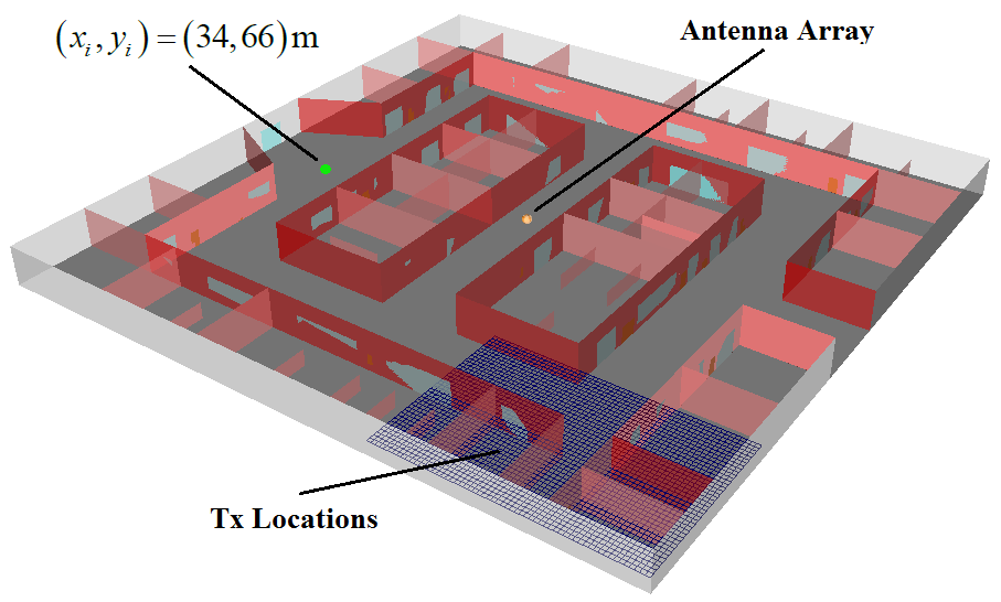
Figure 1: 3D model of a $80\times 80m\times 5m$ floor.

Simulated data: This data consists of 802.11 Wi-Fi signals in an artificial $80m\times 80m$ indoor office environment generated by Kupershtein et al., (2013) using a 3D radio wave propagation software, see Figure 1.

Real data: These are actual 802.11 signals, recorded by a Wi-Fi router placed roughly in the middle of a $27m\!\times\!33m$ office, see Figure B.3 of the supplementary.

The Signal Subspace Projection (SSP) of Kupershtein et al., (2013) and Jaffe and Wax, (2014) is used as the fingerprint for localization. It is based on the assumption that signals received from close locations have similar properties of differential delays and directions of arrival. In our experiments, the SSP features are $48\times 48$ projection matrices, where the projected subspace is 10-dimensional. We use the Frobenius norm as the distance metric and construct a symmetric-4NN graph as described in Section 2. For more details on the datasets and SSP features, see the supplementary.

We compare our semi-supervised geodesic kNN regressor to Laplacian eigenvector regression (Belkin and Niyogi,, 2004). As a baseline we also applied classic kNN regression, using only the labeled samples and optimizing over $k$. Figure 2 shows the median localization error on the simulated data set as a function of the number of unlabeled locations, where the labeled points are placed on a fixed grid. Specifically, for the geodesic kNN regressor we used $k=7$ and exponentially decaying weights such that the weight of the $i$-th neighbor is proportional to $1/2^{i}$. Since the weights decay exponentially, the specific choice of $k$ is not important, with larger values of $k$ giving nearly identical results. For Laplacian eigenvector regression, we optimized over the number of eigenvectors by taking the best outcome after repeating the experiment with $10\%,20\%,30\%,40\%$ and $50\%$ of the labeled points.

Table 1 shows the mean localization error on the real data set for different densities of labeled points. The results on both the simulated and real datasets show a clear advantage for the geodesic kNN regressor. As expected, the improvement shown by the semi-supervised methods increases with the number of unlabeled locations. Moreover geodesic kNN regression is much faster to compute than the Laplacian eigenvector regressor, see Table 2 in the supplementary.

Table 1: Mean accuracy of kNN, geodesic kNN and Laplacian eigenbasis regression on the real data set

Labeled grid	n	kNN	GNN	Laplacian
1.5m	73	1.49m	1.11m	1.36m
2.0m	48	2.27m	1.49m	1.65m
3m	23	3.41m	2.41m	2.79m

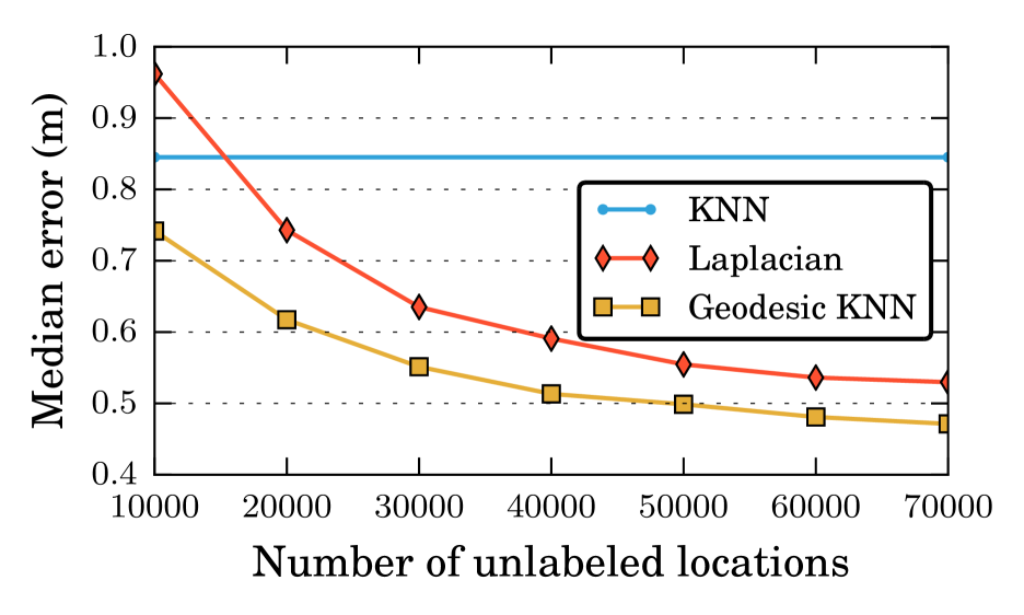
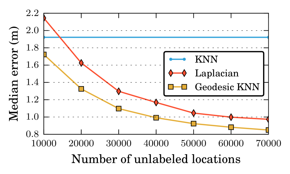
Figure 2: Median localization error vs. number of unlabeled points. Top: $1600$ labeled points placed on a regular grid with a side length of $2m$. Bottom: $400$ labeled points on a $4m$ grid.

5.2 Facial pose estimation

We illustrate the performance of geodesic kNN on another regression problem, using the faces data set where the predicted value is the left-right angle of a face image. This data set contains $698$ greyscale images of a single face rendered at different angles and lighting. The instance space is the set of all $64\times 64$ images whereas the intrinsic manifold dimension is $3$. For our benchmark, we computed the $\ell_{1}$ distance between all pairs of images and constructed a symmetric $4$-NN graph. For the geodesic kNN algorithm, the edge weights were set to the $\ell_{1}$ distances and $k$ was set to 1. For Laplacian eigenvector regression we used binary weights and set the number of eigenvectors to 20% of the number of labeled points. This is a common rule-of-thumb, and gave good results over the whole range.

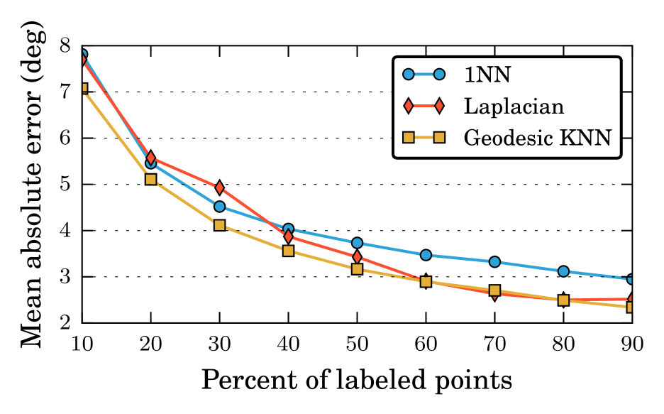
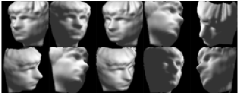
Figure 3: Top: mean prediction error for the left-right angle of the face. Bottom: sample images from the faces data set, showing different poses and lighting.

Figure 3 shows that geodesic kNN performs uniformly better than the nearest neighbor regressor and also outperforms the semi-supervised Laplacian regressor.

Acknowledgments

We would like to thank Mati Wax, Jonathan Rosenblatt, Amit Gruber, Roee David and Jonathan Bauch for interesting discussions about this work and to Evgeny Kupershtein for providing data sets.

Supplementary Material

Appendix A Auxiliary lemmas

Consider a graph $G$ constructed from $\{X_{1},\ldots,X_{N}\}$ as described in Section 2 of the main text. For any ${\bf x}\in\{X_{1},\ldots,X_{N}\}$, denote by $X_{G}^{(\ell)}({\bf x})$ and $X_{\mathcal{M}}^{(\ell)}({\bf x})$ its closest point from $X_{1},\ldots X_{\ell}$ points, according to either the graph or the manifold distance,

$$X_{G}^{(\ell)}({\bf x}) :=\operatorname*{\arg\!\min}_{X_{j}\in\{X_{1},\ldots,X_{\ell}\}}d_{G}(X_{i},X_{j}),$$

$$X_{\mathcal{M}}^{(\ell)}({\bf x}) :=\operatorname*{\arg\!\min}_{X_{j}\in\{X_{1},\ldots,X_{\ell}\}}d_{{\mathcal{M}}}(X_{i},X_{j}).$$

Lemma A.1.

Let $X_{1},\ldots,X_{\ell}\overset{i.i.d.}{\sim}\mu$ and let ${\bf x}\in{\mathcal{M}}$. Assume that $\mu(B_{{\bf x}}(r))\geq Qr^{d}$ for all $r\leq R$. Then for any $\lambda>0$,

$$\int_{0}^{\lambda^{2}R^{2}}\Pr\left[d_{{\mathcal{M}}}\left({\bf x},X_{{\mathcal{M}}}^{(\ell)}({\bf x})\right)>\frac{\sqrt{r}}{\lambda}\right]dr\leq\frac{2\lambda^{2}\ell^{-\frac{2}{d}}}{(1-e^{-Q})^{2}}.$$

Proof.

Substituting $t=\sqrt{r}/\lambda$, the integral becomes

$$\int_{0}^{R}\Pr\left[d_{{\mathcal{M}}}\left({\bf x},X_{{\mathcal{M}}}^{(\ell)}({\bf x})\right)>t\right]2\lambda^{2}tdt.$$ (A.1)

Now, $d_{{\mathcal{M}}}({\bf x},X_{{\mathcal{M}}}^{(\ell)}({\bf x}))>t$ if and only if all $\ell$ samples fall outside the manifold ball $B_{{\bf x}}(t)$. Hence,

$$\Pr\left[d_{{\mathcal{M}}}({\bf x},X_{{\mathcal{M}}}^{(\ell)}({\bf x}))>t\right]=(1-\mu(B_{{\bf x}}(t)))^{\ell}.$$

Since $\mu(B_{{\bf x}}(t))\geq Qt^{d}$ for all $t\leq R$,

$$\Pr\left[d_{{\mathcal{M}}}({\bf x},X_{{\mathcal{M}}}^{(\ell)}({\bf x}))>t\right]\leq(1-Qt^{d})^{\ell}\leq e^{-Qt^{d}\ell}$$ (A.2)

We insert (A.2) into (A.1), extend the domain of integration to $(0,\infty)$ and split it into intervals of length $\ell^{-\frac{1}{d}}$. Each integral is bounded separately using the fact that t is increasing and $e^{-Qt^{d}\ell}$ is decreasing.

$$\int_{0}^{R}t\cdot e^{-Qt^{d}\ell}dt<\sum_{k=0}^{\infty}\int_{k\ell^{-\frac{1}{d}}}^{(k+1)\ell^{-\frac{1}{d}}}t\cdot e^{-Qt^{d}\ell}dt$$

$$\leq\sum_{k=0}^{\infty}\ell^{-\frac{2}{d}}(k+1)\cdot e^{-k^{d}Q}\leq\ell^{-\frac{2}{d}}\sum_{k=0}^{\infty}(k+1)\cdot e^{-kQ}$$

$$=\ell^{-\frac{2}{d}}\left(\sum_{k=0}^{\infty}e^{-kQ}\right)^{2}=\frac{\ell^{-\frac{2}{d}}}{(1-e^{-Q})^{2}}.$$

Inserting this bound into (A.1) concludes the proof. ∎

Lemma A.2.

Consider a fixed point ${\bf x}\in{\mathcal{M}}$ and let ${\bf x}^{*}=\operatorname*{\arg\!\min}_{{\bf x}^{\prime}\in\{X_{1},\ldots,X_{n+m}\}}\|{\bf x}-{\bf x}^{\prime}\|$ be its Euclidean nearest neighbor from the sample. We denote by $A$ the event that all the inequalities in Eq. (4) hold. Conditioned on this event,

$$\mathbb{E}\left[d_{{\mathcal{M}}}^{2}({\bf x}^{*},X_{G}^{(n)}({\bf x}^{*}))\big{|}A\right]\leq c_{1}({\mathcal{M}},\mu,\delta)n^{-\frac{2}{d}}$$ (A.3)

Proof.

Assume that $A$ holds. By applying Eq. (4) twice, we obtain an upper bound on the manifold distance to the closest labeled point in the graph.

$$d_{\mathcal{M}}({\bf x}^{*},X_{\mathcal{M}}^{(n)}({\bf x}^{*}))\geq\frac{d_{G}({\bf x}^{*},X_{\mathcal{M}}^{(n)}({\bf x}^{*}))}{1+\delta}$$ (A.4)

$$\geq\frac{d_{G}({\bf x}^{*},X_{G}^{(n)}({\bf x}^{*}))}{1+\delta}\geq\frac{1-\delta}{1+\delta}d_{\mathcal{M}}({\bf x}^{*},X_{G}^{(n)}({\bf x}^{*}))$$

Now we apply the well-known equality for a non-negative random variable $\mathbb{E}\left[X\right]=\int_{0}^{\infty}\Pr\left[X>r\right]dr$,

$$\mathbb{E}\left[d_{{\mathcal{M}}}^{2}({\bf x}^{*},X_{G}^{(n)}({\bf x}^{*}))\big{|}A\right]$$

$$=\int\Pr\left[d_{{\mathcal{M}}}^{2}({\bf x}^{*},X_{G}^{(n)}({\bf x}^{*}))>r\big{|}A\right]dr$$

$$=\int_{0}^{\text{diam}({\mathcal{M}})^{2}}\Pr\left[d_{{\mathcal{M}}}\left({\bf x}^{*},X_{G}^{(n)}({\bf x}^{*})\right)>\sqrt{r}\big{|}A\right]dr$$

$$\leq\int_{0}^{\text{diam}({\mathcal{M}})^{2}}\Pr\left[d_{{\mathcal{M}}}\left({\bf x}^{*},X_{{\mathcal{M}}}^{(n)}({\bf x}^{*})\right)>\frac{1-\delta}{1+\delta}\sqrt{r}\bigg{|}A\right]dr$$

$$=\int_{0}^{\left(\frac{1+\delta}{1-\delta}\right)^{2}R^{2}}\Pr\left[\ldots\right]dr+\int_{\left(\frac{1+\delta}{1-\delta}\right)^{2}R^{2}}^{\text{diam}({\mathcal{M}})^{2}}\Pr\left[\ldots\right]dr.$$

Lemma A.1 with $\lambda=(1+\delta)/(1-\delta)$ gives a bound on the first integral. For the second integral, the probability inside it is monotonically decreasing, and by Eq. (A.2) it is in particular smaller than $e^{-QR^{d}n}$. Hence,

$$\mathbb{E}\left[d_{{\mathcal{M}}}^{2}({\bf x}^{*},X_{G}^{(n)}({\bf x}^{*}))\big{|}A\right]$$

$$\leq\frac{2(1+\delta)^{2}}{(1-\delta)^{2}(1-e^{-Q})^{2}}n^{-\frac{2}{d}}+\text{diam}({\mathcal{M}})^{2}\cdot e^{-QR^{d}n}.$$

As a function of $n$, the second summand is negligible with respect to the first. Hence Eq. (A.3) follows. ∎

Appendix B Fast computation of transductive geodesic nearest neighbors

In this section we provide more details regarding the efficient computation of geodesic kNN for all vertices in a graph. We begin by proving the correctness of Algorithm 1 and analyzing its runtime. Then, in Section B.3 we present Algorithm 2 by Har-Peled, (2016) which has a tighter bound on the asymptotic running time. Finally, in Section B.4 we test the empirical running time of these algorithms on the simulated WiFi data set.

B.1 Proof of correctness

We start with some auxiliary definitions and lemmas regarding shortest paths. Given an undirected and weighted graph $G$, we denote paths in $G$ by $v_{i}\to v_{j}\to\ldots\to v_{k}$ or simply $v_{i}\rightsquigarrow v_{k}$ when the context makes it clear what path we are referring to. The length of a path is the sum of its edge weights,

$$w(v_{1}\to v_{2}\to\ldots v_{m})=\sum_{i=1}^{m-1}w(v_{i},v_{i+1}).$$

The length of the shortest (geodesic) path between two vertices $v,v^{\prime}\in V$ is denoted by $d_{G}(v,v^{\prime})$. A path $v\rightsquigarrow v^{\prime}$ is called a shortest path if $w(v\rightsquigarrow v^{\prime})=d_{G}(v,v^{\prime})$. The following lemma is the key to the correctness of Algorithms 1 and 2.

Lemma B.1.

Let $v\in V$ be a vertex and let $s$ be its $j$-th nearest labeled vertex. If $s\rightsquigarrow u\rightsquigarrow v$ is a shortest path then $s\in$ NLV$(u,j)$, where NLV$(u,j)$ is the set of $j$ nearest labeled vertices to $u$.

Proof.

Assume by contradiction that there are $j$ labeled nodes $s_{1},\ldots,s_{j}$ such that

$$\forall i:d_{G}(s_{i},u)<d_{G}(s,u).$$

Then

$$d_{G}(s_{i},v) \leq d_{G}(s_{i},u)+d_{G}(u,v)$$ (triangle inequality)

$$<d_{G}(s,u)+d_{G}(u,v)$$ (by assumption)

$$=d_{G}(s,v).$$ (B.1)

where the last equality is derived from the assumption that $u$ is on a shorted path between $s$ and $v$. Eq. (B.1) implies that the vertices $s_{1},\ldots,s_{j}$ are all closer than $s$ to $v$, which contradicts the assumption. ∎

We now continue to the main part of the proof.

Lemma B.2.

For every triplet$(dist,seed,v_{0})$ popped from $Q$ there is a path $seed\rightsquigarrow v_{0}$ of length $dist$.

Proof.

We prove the claim by induction on the elements inserted into $Q$.

Base of the induction: The first $L$ inserts correspond to the labeled vertices $\{(0,s,s):\ s\in\mathcal{L}\}$. For these triplets the claim holds trivially.

Induction step: Any triplet inserted into $Q$ or updated is of the form $(dist+w(v,v_{0}),seed,v)$ where $(dist,seed,v_{0})$ was previously inserted into $Q$. Hence, by the induction hypothesis there exists a path $seed\rightsquigarrow v_{0}$ of length $dist$. Since $v$ is a neighbor of $v_{0}$ with edge weight $w(v_{0},v)$, there exists a path $seed\rightsquigarrow v_{0}\to v$ of length $w(seed\rightsquigarrow v_{0})+\ w(v_{0}\to v)=dist+\ w(v_{0},v)$. ∎

Lemma B.3.

The distances popped from $Q$ in the main loop form a monotone non-decreasing sequence.

Proof.

This follows directly from the fact that $Q$ is a minimum priority queue and that the edge weights are non-negative, hence future insertions or updates will have a priority that is higher or equal to that of an existing element in the queue. ∎

Lemma B.4.

Every time a triplet $(dist,seed,v_{0})$ is popped from $Q$, the following conditions hold

1. If $seed\in NLV(v_{0},k)$ then $dist=d_{G}(seed,v_{0})$.

2. All pairs $(s,v)\in\mathcal{L}\times V$ that satisfy $d_{G}(s,v)<dist$ and $s\in NLV(v,k)$ are in the $visited$ set.

Proof.

We prove both claims simultaneously by induction on the popped triplets.

Base of the induction: The first $L$ triplets are equal to $\{(0,s,s):s\in\mathcal{L}\}$. Part 1 holds since $d_{G}(s,s)=0$. Part 2 holds because there are no paths shorter than 0.

Induction step:

Part 1. (If $seed\in NLV(v_{0},k)$ then $dist=d_{G}(seed,v_{0})$)

By Lemma B.2, $dist$ is the length of an actual path, so it cannot be smaller than the shortest path length $d_{G}(seed,v_{0})$. Assume by contradiction that $d_{G}(seed,v_{0})<dist$. There is some shortest path $seed\rightsquigarrow v_{p}\to v_{0}$ of length $d_{G}(seed,v_{0})$ ($v_{p}$ may be equal to $seed$, but not to $v_{0}$). Clearly $d_{G}(seed,v_{p})\leq d_{G}(seed,v_{0})<dist$ and by Lemma 3.1, $seed\in NLV(v_{p},k)$. Thus by Part 2 of the induction hypothesis $(seed,v_{p})\in visited$. This implies that $(seed,v_{p})$ was visited in a previous iteration. Note that it follows from $seed\in NLV(v_{p},k)$ and from Lemma B.3 that during the visit of $(seed,v_{p})$ the condition $length(kNN[v_{p}])<k$ was true. Therefore the command dec-or-insert$(Q,d_{G}(seed,v_{p})+w(v_{p},v_{0}),seed,v_{0})$ should have been called, but because $seed\rightsquigarrow v_{p}\to v_{0}$ is a shortest path, $d_{G}(seed,v_{p})+w(v_{p},v_{0})=d_{G}(seed,v_{0})$, leading to the conclusion that the triplet $(d_{G}(seed,v_{0}),seed,v_{0})$ must have been inserted into $Q$ in a previous iteration, which leaves two options:

1. Either $(d_{G}(seed,v_{0}),seed,v_{0})$ was never popped from $Q$, in that case it should have been popped from $Q$ in the current iteration instead of $(dist,seed,v_{0})$. Contradiction.

2. The triplet $(d_{G}(seed,v_{0}),seed,v_{0})$ was popped from $Q$ in a previous iteration. However this implies a double visit of $(seed,v_{0})$, which is impossible due to the use of the visited set.

Part 2. (All pairs $(s,v)\in\mathcal{L}\times V$ that satisfy $d_{G}(s,v)<dist$ and $s\in NLV(v,k)$ are contained in $visited$)

Let $(s,v)\in\mathcal{L}\times V$ be a pair of vertices that satisfies $d_{G}(s,v)<dist$ and $s\in NLV(v,k)$. Assume by contradiction that $(s,v)\notin visited$. Let $s\rightsquigarrow v^{\prime}\to v^{\prime\prime}\rightsquigarrow v$ be a shortest path such that $(s,v^{\prime})\in$ visited but $(s,v^{\prime\prime})\notin$ visited. Such $v^{\prime},v^{\prime\prime}$ must exist since $(s,s)\in visited$ and by our assumption $(s,v)\notin visited$. We note that $s$ may be equal to $v^{\prime}$ and $v^{\prime\prime}$ may be equal to $v$. Since $(s,v^{\prime})\in visited$, some triplet $(d,s,v^{\prime})$ was popped from $Q$ in a previous iteration and by Part 1 of the induction hypothesis $d=d_{G}(s,v^{\prime})$. By Lemma 3.1 we know that $s\in NLV(v^{\prime},k)$, therefore during the visit of $(s,v^{\prime})$ the condition $length(kNN[v^{\prime}])<k$ was true. Following this, there must have been a call to decrease-key-or-insert$(Q,d_{G}(s,v^{\prime})+w(v^{\prime},v^{\prime\prime}),s,v^{\prime\prime})$. Now,

$$d_{G}(s,v^{\prime})+w(v^{\prime},v^{\prime\prime})$$

$$=d_{G}(s,v^{\prime\prime}) s\rightsquigarrow v^{\prime}\to v^{\prime\prime}$$ ( is a shortest path)

$$\leq d_{G}(s,v) s\rightsquigarrow v^{\prime\prime}$$ ( is a subpath)

Hence the pair $(s,v^{\prime\prime})$ was previously stored in $Q$ with distance $d_{G}(s,v^{\prime\prime})\leq d_{G}(s,v)<dist$. Since $(s,v^{\prime\prime})\notin$ visited, it should have been present in $Q$ with a smaller distance than $(s,v)$ as key, thus $(d_{G}(s,v^{\prime\prime}),s,v^{\prime\prime})$ should have been popped instead of $(dist,seed,v_{0})$, contradiction. ∎

Finally, we are ready to state the theorem that Algorithm 1 produces correct output, namely that its output for every vertex $v\in V$ is indeed the set of its $k$ nearest labeled points, as measured by the geodesic graph distance.

Theorem B.1.

Let $G=(V,E,w)$ be a graph with non-negative weights. For every vertex $v\in V$ let $\mathcal{L}_{v}$ denote the set of labeled vertices in the connected component of $v$ and let $\ell_{v}=\min\{k,|\mathcal{L}_{v}|\}$. Then

1. Algorithm 1 stops after a finite number of steps.

2. Once stopped, for every $v\in V$ the output list $kNN[v]$ is of the form $kNN[v]=[(d_{G}(s_{1},v),s_{1}),\ldots,(d_{G}(s_{\ell},v),s_{\ell_{v}})]$ where $s_{1},\ldots,s_{\ell_{v}}$ are the nearest labeled vertices, sorted by their distance to $v$.

Proof.

Part 1 follows trivially from the fact that every pair $(seed,v_{0})$ can be popped at most once and part 2 follows from Lemma B.4 and an induction on the popped triplets $(d,s,v)$. ∎

B.2 Transductive runtime analysis of Algorithm 1

Lemma B.1 explains why Algorithm 1 can stop exploring the neighbors of vertices whose $k$ nearest labeled neighbors were found. As Theorem B.2 shows, this can lead to dramatic runtime savings.

Theorem B.2.

Given a graph $G=(V,E)$ with $n$ labeled vertices, the runtime of Algorithm 1 is bounded by $O\left(k|E|+N_{p}\log|V|\right)$ where $N_{p}$ is the total number of pop-minimum operations, which satisfies $N_{p}\leq\min\{n|V|,k|E|\}$.

Proof.

Recall that in a priority queue based on a Fibonacci heap all operations cost $O(1)$ amortized time except pop-minimum which costs $\log|Q|$. The runtime is dominated by the cost of all pop-minimum operations, plus the total cost of traversing the neighbors of the examined vertices. The latter takes $O(k|E|)$ time. Denote the total number of pop-minimum operations by $N_{p}$. We derive two different bounds on $N_{p}$. Every time a $(seed,v)$ pair is popped from $Q$, it is added to the $visited$ set, which prevents future insertions of that pair into $Q$. Hence, each pair $(seed,v)\in\mathcal{L}\times V$ may be popped at most once from $Q$, which implies that $N_{p}\leq n|V|.$ In addition, $N_{p}$ is bounded by the number of insertions into $Q$. First, there are $n$ insertions during the initialization phase. Then, for each vertex $v_{0}\in V$, the "if $length(kNN[v_{0}])<k$" clause can hold true at most $k$ times for that vertex. Each time, the neighbors of $v_{0}$ are examined and up to $deg(v_{0})$ neighbors are inserted into $Q$. This yields the second bound, $N_{p}\leq n+k|E|=O(k|E|).$ ∎

B.3 Saving unneeded extractions

Algorithm 1 keeps a priority queue with pairs $(seed,v)\in\mathcal{L}\times V$. However, once a vertex $v$ has been visited from $k$ different seed vertices, we no longer need to process it further. Thus any later pop operations which involve $v$ are a waste of CPU cycles. Conceptually, once $v$ is visited for the $k$^th time, we would like to purge the queue of all pairs $(s,v)$, but this is expensive since every pop operation costs $\log|Q|$. Instead we use an idea by Har-Peled, (2016), which we detail in Algorithm 2. For every vertex $v\in V$ we keep a separate priority queue $Q_{v}$, which will be disabled once $v$ is visited $k$ times. A global priority queue $Q$ is maintained that keeps the lowest element of each of the local queues $Q_{v}$. Now popping an element involves popping some $v$ from $Q$ and then popping $Q_{v}$. This is followed by an insert of the new minimum element from $Q_{v}$ into $Q$.

Algorithm 2 Geodesic k nearest labeled neighbors with faster priority queue handling

Input:

An undirected weighted graph $G=(V,E,w)$ and a set of labeled vertices $\mathcal{L}\subseteq V$.

Output: For every $v\in V$ a list $kNN[v]$ with the $k$ nearest labeled vertices to $v$ and their distances.

  $Q\leftarrow$PriorityQueue()

  for $v\in V$ do

        $Q_{v}\leftarrow$PriorityQueue()

        kNN[$v$] $\leftarrow$ Empty-List()

        $S_{v}\leftarrow\phi$

        if $v\in\mathcal{L}$ then

              insert($Q$, $v$, priority = 0)

              insert($Q_{v}$, $v$, priority = 0)  

  while $Q\neq\phi$ do

        ($v_{0}$, dist) $\leftarrow$ pop-minimum($Q$)

        (seed, dist) $\leftarrow$ pop-minimum($Q_{v_{0}}$)

        $S_{v_{0}}\leftarrow S_{v_{0}}\ \cup\ \{$seed$\}$

        append (seed, dist) to kNN[$v_{0}$]

        if length(kNN[$v_{0}$]) < $k$ and $Q_{v_{0}}\neq\phi$ then

              (newseed, newdist) $\leftarrow$ minimum($Q_{v_{0}}$)

              insert($Q$, $v_{0}$, priority = newdist)

        for all $v\in$ neighbors($v_{0}$) do

              if length(kNN[$v$]) < $k$ and seed $\notin S_{v}$ then

                    decrease-or-insert($Q_{v}$, seed,    priority = dist $+w(v_{0},v)$)

                    decrease-or-insert($Q$, $v$,     priority = dist $+w(v_{0},v)$)

Theorem B.3.

Given a graph $G=(V,E)$ with $n$ labeled vertices, the runtime of Algorithm 2 is bounded by $O\left(k|E|+kV\log|V|\right)$

Proof.

The runtime of Algorithm 2 is bounded by $O\left(k|E|+N_{p}\log|V|\right)$. Let $v\in V$ be a vertex. Pairs of the form $(seed,v)$ may be popped at most $k$ times. hence $N_{p}\leq k|V|$. ∎

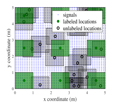
Figure B.1: Schematic of the labeled and unlabeled point generation for the simulated data set. Labeled locations (green circles) were placed on a $4m$ grid, whereas the unlabeled locations (grey circles) were placed at random. The signature of a location is computed by Eq. (C.1) using all the signals in a 1m square neighborhood of the location.

An immediate corollary of Theorem B.3 is that for a graph $G=(V,E)$ of bounded degree $d$, the runtime of Algorithm 2 is $O(k|V|\log|V|).$ In contrast, the runtime of the naïve approach based on multiple Dijkstra runs is $O\left(n|V|\log|V|\right)$. Comparing these two formulas, we see that major speedups are obtained in typical cases where $n\gg k$. As we illustrate empirically in the following Section, these speedups are very large in practice, even on graphs of moderate size.

B.4 Empirical runtime comparison

We compare the runtime of Algorithms 1 and 2 to the naïve method of running Dijkstra’s algorithm from each of the labeled points. To make the comparison meaningful we implemented all of these algorithms in Python, using a similar programming style and the same heap data structure. The running times were measured for the simulated WiFi signals data set. Figure B.2 shows the relative speedup (measured in seconds) of both algorithms compared to multiple Dijkstra runs. Interestingly, while Algorithm 2 has better asymptotic guarantees than Algorithm 1, both show similar speedups on this particular data set.

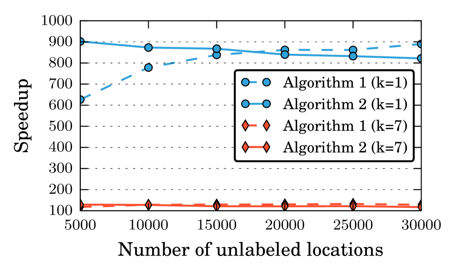
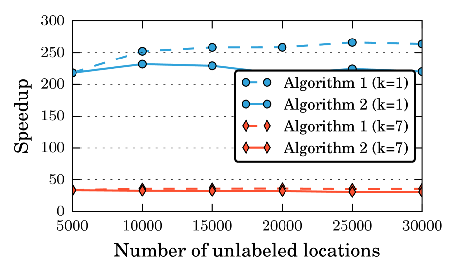
Figure B.2: Relative speedup computing the geodesic 1NN and 7NN of all points in a graph using Algorithms 1 and 2. The speedup of both algorithms is compared to the naïve approach of running Dijkstra’s algorithm from each labeled point. Top panel: $1600$ labeled locations are placed on a 2m square grid. Bottom panel: $400$ labeled locations placed on a 4m grid.

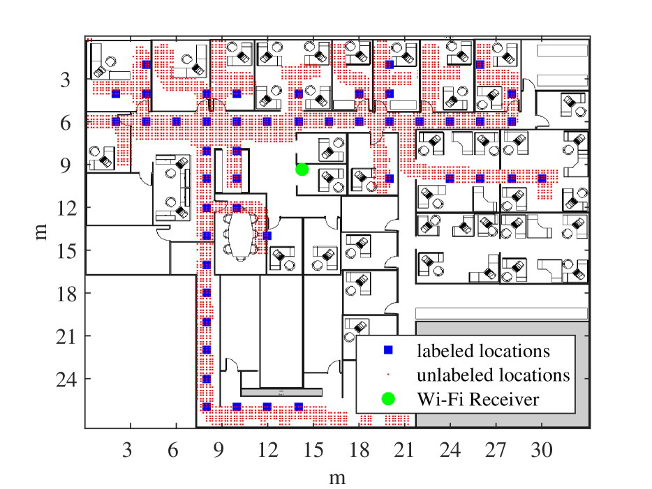
Figure B.3: Schematic of the mapped areas in the real data set

Table 2: Runtime of Geodesic 7-NN vs. time to compute Laplacian eigenvectors

#unlabeled	G7NN	Laplacian	Graph build
1000	2.3s	7.6s	9s
10000	7s	195s	76s
100000	56s	114min	66min

Table 2 compares the runtime of the geodesic 7NN method to the runtime of computing the top eigenvectors of the Laplacian matrix, using the simulated indoor localization data set with labeled locations every $2m$. The number of eigenvectors was chosen to be $320$, which is equal to 20% of the number of labeled points. Computing the geodesic nearest neighbors by using Algorithm 1 is several orders of magnitude faster than computing the eigenvectors. This is despite the fact that the eigenvector computation is performed using the highly optimized Intel^® Math Kernel Library whereas the geodesic nearest neighbor computation uses a simple Python implementation. We expect an efficient implementation of geodesic kNN to be at least 10 times faster. For completeness, the third column shows the graph construction time, using the naïve $O(n^{2})$ algorithm.

Appendix C Indoor localization details

C.1 Dataset description

Simulated data: This data consists of 802.11 Wi-Fi signals in an artificial yet realistic environment generated by Kupershtein et al., (2013) using a 3D radio wave propagation software. The environment is an $80m\times\!80m$ floor. In its center is a Wi-Fi router with $p=6$ antennas. See Figure 1. At various locations $(x,y)\in\mathbb{R}^{2}$, $N=8$ consecutive samples of a Wi-Fi packet’s (constant) preamble are recorded, at equally spaced time intervals of $50\mu s$. The samples are stored in a complex-valued vector $s_{x,y}\in\mathbb{C}^{pN}$ which we refer to as the signal received from location $(x,y)$. The simulated signals were generated on a dense $0.1m$ grid covering the entire area of the floor.

Real data: This data consists of actual 802.11 signals, recorded by a Wi-Fi router with $p=6$ antennas placed approximately in the middle of a $27m\!\times\!33m$ office, see Figure B.3. The transmitter was a tablet connected to the router via Wi-Fi. The signal vector of each location $(x,y)$ was sampled $N=8$ times from every antenna. The transmitter locations were entered manually by the operator. For both the labeled and unlabeled locations, we first generated a square grid covering the area of the office, and then kept only the locations that contained received signals. For the labeled points, we repeated the experiments with several grid sizes ranging from $1.5m$ to $3m$. The location of the WiFi router is marked by the green circle.

C.2 Feature extraction and distance metric for the SSP method

The Signal Subspace Projection method is based on the assumption that signals originating from nearby locations are high dimensional vectors contained in a low dimensional subspace. Hence, signals originating from nearby locations are contained in a low dimensional subspace. The subspace around each location is used as its signature. Specifically, the signature $P_{\ell}$ of a location $\ell=(x,y)\in\mathbb{R}^{2}$ is computed as follows. First, the covariance matrix of the signals in the proximity of $\ell$ is computed, using all the signals in the dataset that are inside a $1m$ square around $\ell$ (see Figure B.1),

$$R_{\ell}:=\sum_{\ell^{\prime}\in\mathbb{R}^{2}:\|\ell-\ell^{\prime}\|_{\infty}<0.5m}s_{\ell^{\prime}}s_{\ell^{\prime}}^{*}$$ (C.1)

where $s_{\ell^{\prime}}^{*}$ denotes the Hermitian transpose of the column vector $s_{\ell^{\prime}}\in\mathbb{C}^{pN}$. Next, we compute the $n_{pc}$ leading eigenvectors of $R_{\ell}$, forming a matrix $V_{\ell}\in\mathbb{C}^{pN\times n_{pc}}$. The SSP signature is the projection matrix onto the space spanned by these eigenvectors, $P_{\ell}:=V_{\ell}V_{\ell}^{*}$. In our experiments, we picked $n_{pc}=10$, though other choices in the range $\{8,\ldots,12\}$ gave results that are almost as good. The distance between pairs of locations is defined as the Frobenius norm of the difference of their projection matrices, $d_{i,j}:=\|P_{\bf\ell_{i}}-P_{\bf\ell_{j}}\|_{F}.$ gave us results that are on par with the best methods of Jaffe and Wax, (2014).

For the simulated dataset, to mimic how a real-world semi-supervised localization system might work, we generated the labeled locations on a regular square grid, whereas the unlabeled locations were randomly distributed over the entire area of the floor (see Figure B.1). For the real dataset, due to physical constraints, labeled and unlabeled points were not placed on a regular grid. Then, we created a symmetric kNN graph by connecting every point $x_{i}$ with its $k_{G}$ closest neighbors, with corresponding weights given by $w_{i,j}=1+\epsilon d_{i,j}$. Here $\epsilon>0$ is a small constant which gives preference to paths with smaller $d_{i,j}$. Experimentally using the symmetric kNN graph construction with $k=4$ gave slightly better results than choosing $k\in\{3,5,6\}$ for both the geodesic kNN regressor and for the Laplacian eigenvector regressor.

References

- Alamgir and von Luxburg, (2012) Alamgir, M. and von Luxburg, U. (2012). Shortest path distance in random k-nearest neighbor graphs. International Conference on Machine Learning (ICML).
- Andoni and Indyk, (2006) Andoni, A. and Indyk, P. (2006). Near-optimal hashing algorithms for approximate nearest neighbor in high dimensions. In The IEEE Symposium on Foundations of Computer Science (FOCS), pages 459–468.
- Belkin and Niyogi, (2004) Belkin, M. and Niyogi, P. (2004). Semi-Supervised Learning on Riemannian Manifolds. Machine Learning, 56:209–239.
- Bentley, (1975) Bentley, J. L. (1975). Multidimensional binary search trees used for associative searching. Communications of the ACM, 18(9):509—-517.
- Bickel and Li, (2007) Bickel, P. J. and Li, B. (2007). Local polynomial regression on unknown manifolds. In Tomography, Networks and Beyond, pages 177–186. Institute of Mathematical Statistics.
- Bijral et al., (2011) Bijral, A. S., Ratliff, N., and Srebro, N. (2011). Semi-supervised Learning with Density Based Distances. In Conference on Uncertainty in Artificial Intelligence (UAI), pages 43–50.
- Chapelle et al., (2006) Chapelle, O., Schölkopf, B., and Zien, A. (2006). Semi-Supervised Learning. MIT Press Cambridge.
- Chapelle and Zien, (2005) Chapelle, O. and Zien, A. (2005). Semi-Supervised Classification by Low Density Separation. In International Conference on Artificial Intelligence and Statistics (AISTATS), pages 57–64.
- Dasgupta et al., (2006) Dasgupta, S., Papadimitriou, C. H., and Vazirani, U. (2006). Algorithms. McGraw-Hill, Inc.
- Erwig, (2000) Erwig, M. (2000). The graph Voronoi diagram with applications. Networks, 36:156–163.
- Goldberg et al., (2009) Goldberg, A. B., Zhu, X., Singh, A., Xu, Z., and Nowak, R. D. (2009). Multi-manifold semi-supervised learning. In International Conference on Artificial Intelligence and Statistics (AISTATS).
- Györfi et al., (2002) Györfi, L., Kohler, M., Krzyżak, A., and Walk, H. (2002). A distribution-free theory of nonparametric regression. Springer Series in Statistics. Springer-Verlag, New York.
- Har-Peled, (2016) Har-Peled, S. (2016). Computing the k Nearest-Neighbors for all Vertices via Dijkstra. ArXiv e-prints.
- Jaffe and Wax, (2014) Jaffe, A. and Wax, M. (2014). Single-Site Localization via Maximum Discrimination Multipath Fingerprinting. IEEE Transactions on Signal Processing, 62(7):1718–1728.
- Kpotufe, (2011) Kpotufe, S. (2011). k -NN Regression Adapts to Local Intrinsic Dimension. In Neural Information Processing Systems (NIPS).
- Kupershtein et al., (2013) Kupershtein, E., Wax, M., and Cohen, I. (2013). Single-site emitter localization via multipath fingerprinting. IEEE Transactions on Signal Processing, 61(1):10–21.
- Lafferty and Wasserman, (2007) Lafferty, J. and Wasserman, L. (2007). Statistical analysis of semi-supervised regression. In Neural Information Processing Systems (NIPS).
- Lee, (2012) Lee, J. M. (2012). Introduction to Smooth Manifolds. Springer New York.
- Liu et al., (2007) Liu, H., Darabi, H., Banerjee, P., and Liu, J. (2007). Survey of wireless indoor positioning techniques and systems. IEEE Transactions on Systems, Man and Cybernetics Part C: Applications and Reviews, 37(6):1067–1080.
- Niyogi, (2013) Niyogi, P. (2013). Manifold Regularization and Semi-supervised Learning: Some Theoretical Analyses. Journal of Machine Learning Research (JMLR), 14(1):1229–1250.
- Omohundro, (1989) Omohundro, S. M. (1989). Five balltree construction algorithms. Technical report, International Computer Science Institute.
- Rigollet, (2007) Rigollet, P. (2007). Generalization error bounds in semi-supervised classification under the cluster assumption. Journal of Machine Learning Research (JMLR), 8:1369–1392.
- Singh et al., (2009) Singh, A., Nowak, R., and Zhu, X. (2009). Unlabeled data: Now it helps, now it doesn’t. Neural Information Processing Systems (NIPS), pages 1513–1520.
- Subramanya and Talukdar, (2014) Subramanya, A. and Talukdar, P. P. (2014). Graph-Based Semi-Supervised Learning. Synthesis Lectures on Artificial Intelligence and Machine Learning, 8(4):1–125.
- Tenenbaum et al., (2000) Tenenbaum, J. B., De Silva, V., and Langford, J. C. (2000). A global geometric framework for nonlinear dimensionality reduction. Science (New York, N.Y.), 290(5500):2319–2323.
- Ting et al., (2010) Ting, D., Huang, L., and Jordan, M. I. (2010). An Analysis of the Convergence of Graph Laplacians. In International Conference on Machine Learning (ICML), pages 1079–1086.
- Tsybakov, (2009) Tsybakov, A. B. (2009). Introduction to nonparametric estimation. Springer New York.
- Wang et al., (2013) Wang, D., Shi, L., and Cao, J. (2013). Fast algorithm for approximate k-nearest neighbor graph construction. In 2013 IEEE 13th International Conference on Data Mining Workshops.
- Zhang et al., (2013) Zhang, Y.-M., Huang, K., Geng, G., and Liu, C.-L. (2013). Fast kNN graph construction with locality sensitive hashing. In Proceedings of the European Conference on Machine Learning and Principles and Practice of Knowledge Discovery in Databases (ECML PKDD), pages 660–674.
- Zhu et al., (2003) Zhu, X., Ghahramani, Z., and Lafferty, J. (2003). Semi-supervised learning using gaussian fields and harmonic functions. International Conference on Machine Learning (ICML).
- Zhu et al., (2009) Zhu, X., Goldberg, A. B., Brachman, R., and Dietterich, T. (2009). Introduction to Semi-Supervised Learning. Morgan and Claypool Publishers.