Normalizing Flows on Riemannian Manifolds

Abstract

We consider the problem of density estimation on Riemannian manifolds. Density estimation on manifolds has many applications in fluid-mechanics, optics and plasma physics and it appears often when dealing with angular variables (such as used in protein folding, robot limbs, gene-expression) and in general directional statistics. In spite of the multitude of algorithms available for density estimation in the Euclidean spaces $\mathbf{R}^{n}$ that scale to large n (e.g. normalizing flows, kernel methods and variational approximations), most of these methods are not immediately suitable for density estimation in more general Riemannian manifolds. We revisit techniques related to homeomorphisms from differential geometry for projecting densities to sub-manifolds and use it to generalize the idea of normalizing flows to more general Riemannian manifolds. The resulting algorithm is scalable, simple to implement and suitable for use with automatic differentiation. We demonstrate concrete examples of this method on the n-sphere $\mathbf{S}^{n}$.

In recent years, there has been much interest in applying variational inference techniques to learning large scale probabilistic models in various domains, such as images and text [1, 2, 3, 4, 5, 6]. One of the main issues in variational inference is finding the best approximation to an intractable posterior distribution of interest by searching through a class of known probability distributions. The class of approximations used is often limited, e.g., mean-field approximations, implying that no solution is ever able to resemble the true posterior distribution. This is a widely raised objection to variational methods, in that unlike MCMC, the true posterior distribution may not be recovered even in the asymptotic regime. To address this problem, recent work on Normalizing Flows [7], Inverse Autoregressive Flows [8], and others [9, 10] (referred collectively as normalizing flows), focused on developing scalable methods of constructing arbitrarily complex and flexible approximate posteriors from simple distributions using transformations parameterized by neural networks, which gives these models universal approximation capability in the asymptotic regime. In all of these works, the distributions of interest are restricted to be defined over high dimensional Euclidean spaces.

There are many other distributions defined over special homeomorphisms of Euclidean spaces that are of interest in statistics, such as Beta and Dirichlet (n-Simplex); Norm-Truncated Gaussian (n-Ball); Wrapped Cauchy and Von-Misses Fisher (n-Sphere), which find little applicability in variational inference with large scale probabilistic models due to the limitations related to density complexity and gradient computation [11, 12, 13, 14]. Many such distributions are unimodal and generating complicated distributions from them would require creating mixture densities or using auxiliary random variables. Mixture methods require further knowledge or tuning, e.g. number of mixture components necessary, and a heavy computational burden on the gradient computation in general, e.g. with quantile functions [15]. Further, mode complexity increases only linearly with mixtures as opposed to exponential increase with normalizing flows. Conditioning on auxiliary variables [16] on the other hand constrains the use of the created distribution, due to the need for integrating out the auxiliary factors in certain scenarios. In all of these methods, computation of low-variance gradients is difficult due to the fact that simulation of random variables cannot be in general reparameterized (e.g. rejection sampling [17]). In this work, we present methods that generalizes previous work on improving variational inference in $\mathbf{R}^{n}$ using normalizing flows to Riemannian manifolds of interest such as spheres $\mathbf{S}^{n}$, tori $\mathbf{T}^{n}$ and their product topologies with $\mathbf{R}^{n}$, like infinite cylinders.

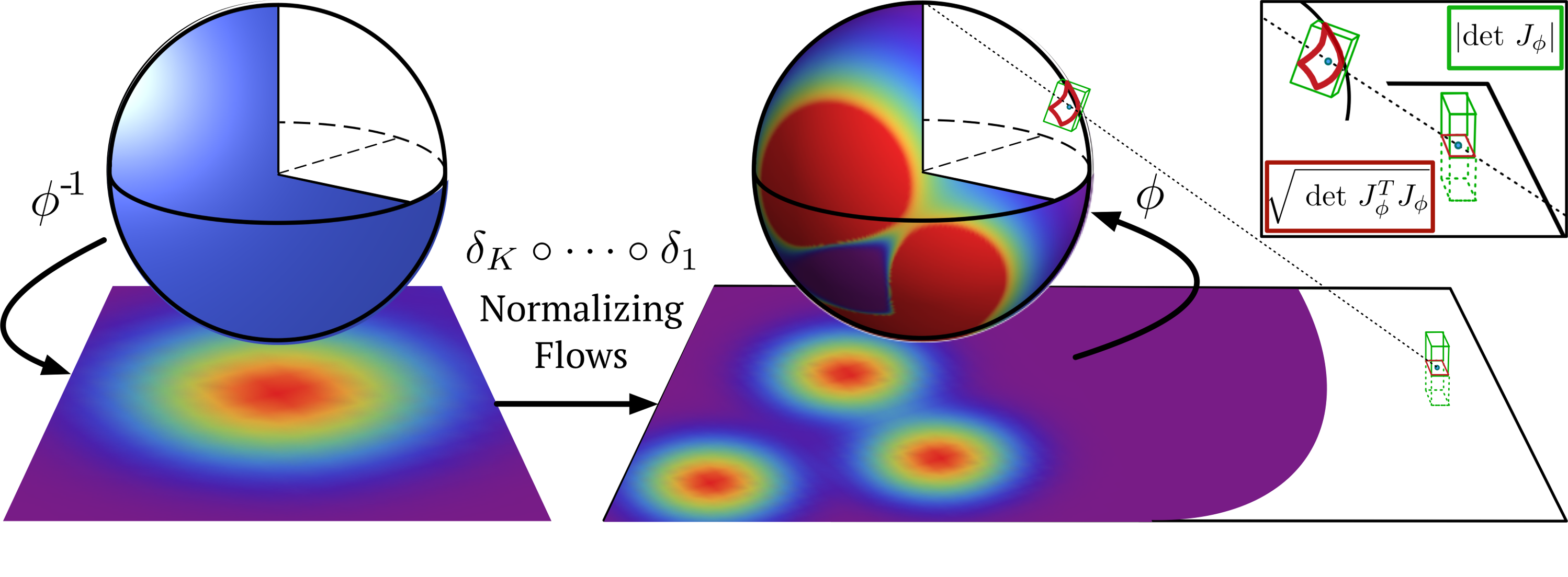
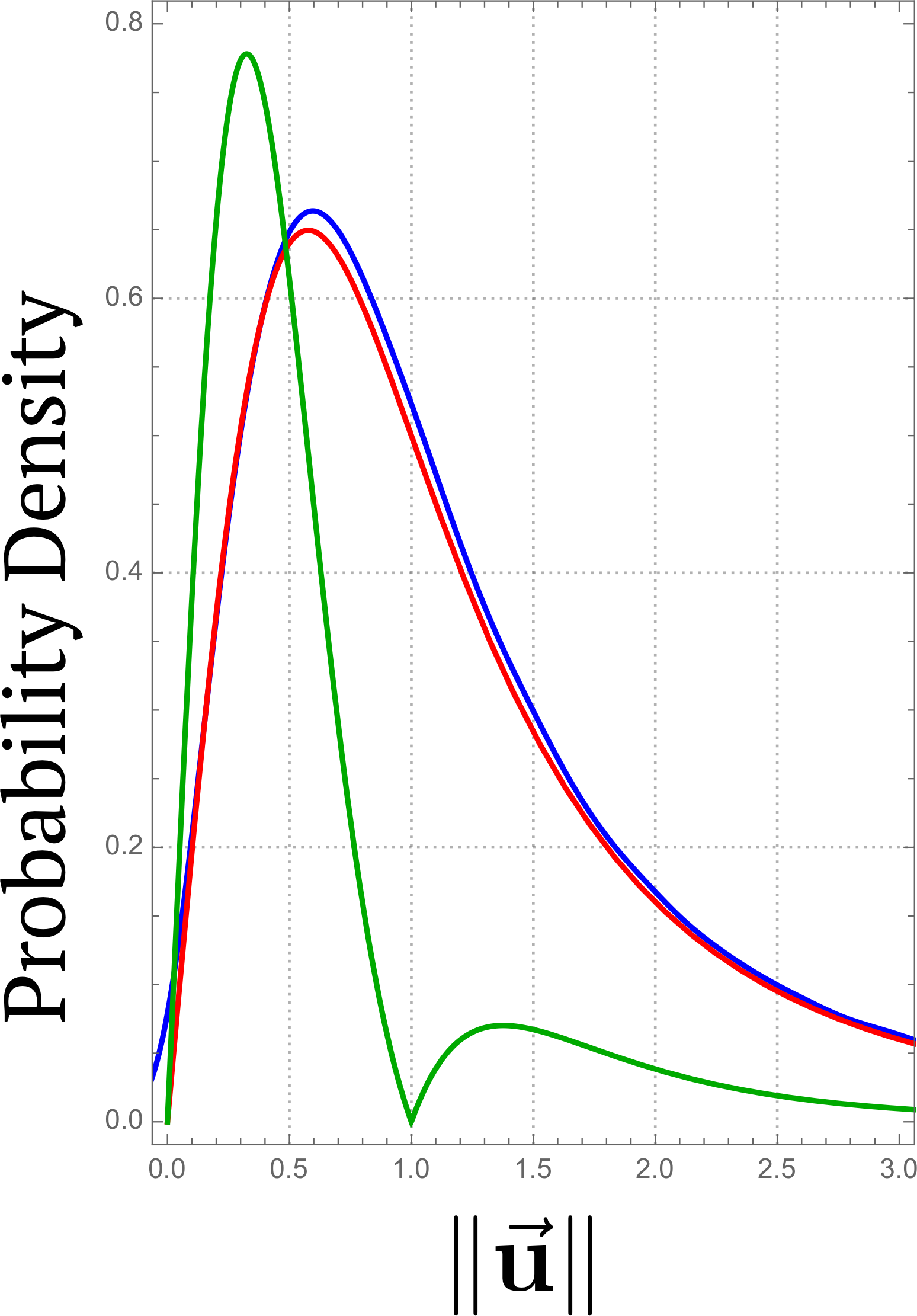
Figure 1: Left: Construction of a complex density on $\mathbf{S}^{n}$ by first projecting the manifold to $\mathbf{R}^{n}$, transforming the density and projecting it back to $\mathbf{S}^{n}$. Right: Illustration of transformed ($\mathbf{S}^{2}\rightarrow\mathbf{R}^{2}$) densities corresponding to an uniform density on the sphere. Blue: empirical density (obtained by Monte Carlo); Red: Analytical density from equation (6); Green: Density computed ignoring the intrinsic dimensionality of $\mathbf{S}^{n}$.

These special manifolds $\mathbf{M}\subset\mathbf{R}^{m}$ are homeomorphic to the Euclidean space $\mathbf{R}^{n}$ where $n$ corresponds to the dimensionality of the tangent space of $\mathbf{M}$ at each point. A homeomorphism is a continuous function between topological spaces with a continuous inverse (bijective and bicontinuous). It maps point in one space to the other in a unique and continuous manner. An example manifold is the unit 2-sphere, the surface of a unit ball, which is embedded in $\mathbf{R}^{3}$ and homeomorphic to $\mathbf{R}^{2}$ (see Figure 1).

In normalizing flows, the main result of differential geometry that is used for computing the density updates is given by, $\mathbf{d}\vec{\mathbf{x}}=|\text{det }J_{\boldsymbol{\phi}}|\text{ }\mathbf{d}\vec{\mathbf{u}}$ and represents the relationship between differentials (infinitesimal volumes) between two equidimensional Euclidean spaces using the Jacobian of the function $\boldsymbol{\phi}:\mathbf{R}^{n}\rightarrow\mathbf{R}^{n}$ that transforms one space to the other. This result only applies to transforms that preserve the dimensionality. However, transforms that map an embedded manifold to its intrinsic Euclidean space, do not preserve the dimensionality of the points and the result above become obsolete. Jacobian of such transforms $\boldsymbol{\phi}:\mathbf{R}^{n}\rightarrow\mathbf{R}^{m}$ with $m>n$ are rectangular and an infinitesimal cube on $\mathbf{R}^{n}$ maps to an infinitesimal parallelepiped on the manifold. The relation between these volumes is given by $\mathbf{d}\vec{\mathbf{x}}=\sqrt{\text{ }\text{det }\mathbf{G}}\text{ }\mathbf{d}\vec{\mathbf{u}}$, where $\mathbf{G}=J_{\boldsymbol{\phi}}^{T}J_{\boldsymbol{\phi}}$ is the metric induced by the embedding $\boldsymbol{\phi}$ on the tangent space $T_{x}\mathbf{M}$, [18, 19, 20]. The correct formula for computing the density over $\mathbf{M}$ now becomes :

$$\int_{\mathbf{M}\subset\mathbf{R}^{m}}\mathbf{f}(\vec{\mathbf{x}})\mathbf{d}\vec{\mathbf{x}}=\int_{\mathbf{R}^{n}}(\mathbf{f}\circ\boldsymbol{\phi})(\vec{\mathbf{u}})\text{ }\sqrt{\text{ }\text{det }\mathbf{G}}\text{ }\mathbf{d}\vec{\mathbf{u}}=\int_{\mathbf{R}^{n}}(\mathbf{f}\circ\boldsymbol{\phi})(\vec{\mathbf{u}})\left(\sqrt{\text{ }\text{det }J_{\boldsymbol{\phi}}^{T}J_{\boldsymbol{\phi}}}\text{ }\right)\mathbf{d}\vec{\mathbf{u}}$$ (1)

The density update going from the manifold to the Euclidian space, $\vec{\mathbf{x}}\in\mathbf{S}^{n}\rightarrow\vec{\mathbf{u}}\in\mathbf{R}^{n}$, is then given by:

$$\mathbf{p}(\vec{\mathbf{u}})=(\mathbf{f}\circ\boldsymbol{\phi})(\vec{\mathbf{u}})\sqrt{\text{ }\text{det }J_{\boldsymbol{\phi}}^{T}J_{\boldsymbol{\phi}}(\vec{\mathbf{u}})}\text{ }=\mathbf{f}(\vec{\mathbf{x}})\sqrt{\text{ }\text{det }J_{\boldsymbol{\phi}}^{T}J_{\boldsymbol{\phi}}(\boldsymbol{\phi}^{-1}(\vec{\mathbf{x}}))}\text{ }$$ (2)

As an application of this method on the $n$-sphere $\mathbf{S}^{n}$, we introduce Inverse Stereographic Transform and define it as: $\boldsymbol{\phi}(\mathbf{u}):\mathbf{R}^{n}\rightarrow\mathbf{S}^{n}\subset\mathbf{R}^{n+1}$,

$$\vec{\mathbf{x}}=\boldsymbol{\phi}(\vec{\mathbf{u}})=\left[\begin{array}[]{c}2\mathbf{u}/(\mathbf{u}^{T}\mathbf{u}+1)\\ 1-2/(\mathbf{u}^{T}\mathbf{u}+1)\\ \end{array}\right]$$ (5)

which maps $\mathbf{R}^{n}$ to $\mathbf{S}^{n}$ in a bijective and bicontinuous manner. The determinant of the metric $\mathbf{G}(\mathbf{x})$ associated with this transformation is given by:

$$\text{det }\mathbf{G}=\text{det }{{J_{\boldsymbol{\phi}}}(\mathbf{x})}^{T}{J_{\boldsymbol{\phi}}}(\mathbf{x})=\text{}\left(\frac{2}{\mathbf{x}^{T}\mathbf{x}+1}\right)^{2n}$$ (6)

Using these formulae, on the left side of Figure 1, we map a uniform density on $\mathbf{S}^{2}$ to $\mathbf{R}^{2}$, enrich this density, using e.g. normalizing flows, and then map it back onto $\mathbf{S}^{2}$ to obtain a multi-modal (or arbitrarily complex) density on the original sphere. On the right side of Figure 1, we show that the density update based on the Riemannian metric, i.e. $\sqrt{\text{ }\text{det }J_{\boldsymbol{\phi}}^{T}J_{\boldsymbol{\phi}}}\text{ }$ (red), is correct and closely follows the kernel density estimate based on 500k samples (blue). We also show that using the generic volume transformation formulation for dimensionality preserving transforms, i.e. $|\text{det }J_{\boldsymbol{\phi}}|\text{ }$ (green), leads to an erroneous density and do not resemble the empirical distributions of samples after the transformation.

References

- [1] D. J. Rezende, S. Mohamed, and D. Wierstra. Stochastic backpropagation and approximate inference in deep generative models. In ICML, 2014.
- [2] D. P. Kingma and M. Welling. Auto-encoding variational Bayes. In ICLR, 2014.
- [3] Karol Gregor, Ivo Danihelka, Alex Graves, Danilo Jimenez Rezende, and Daan Wierstra. Draw: A recurrent neural network for image generation. In ICML, 2015.
- [4] SM Eslami, Nicolas Heess, Theophane Weber, Yuval Tassa, Koray Kavukcuoglu, and Geoffrey E Hinton. Attend, infer, repeat: Fast scene understanding with generative models. arXiv preprint arXiv:1603.08575, 2016.
- [5] Danilo Jimenez Rezende, Shakir Mohamed, Ivo Danihelka, Karol Gregor, and Daan Wierstra. One-shot generalization in deep generative models. In ICML, 2016.
- [6] Matthew D. Hoffman, David M. Blei, Chong Wang, and John Paisley. Stochastic variational inference. Journal of Machine Learning Research, 14:1303–1347, 2013.
- [7] Danilo Jimenez Rezende and Shakir Mohamed. Variational inference with normalizing flows. arXiv preprint arXiv:1505.05770, 2015.
- [8] Diederik P. Kingma, Tim Salimans, and Max Welling. Improving variational inference with inverse autoregressive flow. CoRR, abs/1606.04934, 2016.
- [9] Laurent Dinh, Jascha Sohl-Dickstein, and Samy Bengio. Density estimation using real nvp. 2016.
- [10] Tim Salimans, Diederik P. Kingma, and Max Welling. Markov chain monte carlo and variational inference: Bridging the gap. In Francis R. Bach and David M. Blei, editors, ICML, volume 37 of JMLR Workshop and Conference Proceedings, pages 1218–1226. JMLR.org, 2015.
- [11] Arindam Banerjee, Inderjit S. Dhillon, Joydeep Ghosh, and Suvrit Sra. Clustering on the unit hypersphere using von mises-fisher distributions. J. Mach. Learn. Res., 6:1345–1382, December 2005.
- [12] Siddharth Gopal and Yiming Yang. Von mises-fisher clustering models. In Tony Jebara and Eric P. Xing, editors, Proceedings of the 31st International Conference on Machine Learning (ICML-14), pages 154–162. JMLR Workshop and Conference Proceedings, 2014.
- [13] Marco Fraccaro, Ulrich Paquet, and Ole Winther. Indexable probabilistic matrix factorization for maximum inner product search. In Proceedings of the Thirtieth AAAI Conference on Artificial Intelligence, February 12-17, 2016, Phoenix, Arizona, USA., pages 1554–1560, 2016.
- [14] Arindam Banerjee, Inderjit Dhillon, Joydeep Ghosh, and Suvrit Sra. Generative model-based clustering of directional data. In Proceedings of the Ninth ACM SIGKDD International Conference on Knowledge Discovery and Data Mining, KDD ’03, pages 19–28, New York, NY, USA, 2003. ACM.
- [15] Alex Graves. Stochastic backpropagation through mixture density distributions. CoRR, abs/1607.05690, 2016.
- [16] Lars Maaloe, Casper Kaae Sonderby, Soren Kaae Sonderby, and Ole Winther. Auxiliary deep generative models. CoRR, abs/1602.05473, 2016.
- [17] Scott W. Linderman David M. Blei Christian A. Naesseth, Francisco J. R. Ruiz. Rejection sampling variational inference. 2016.
- [18] Adi Ben-Israel. The change-of-variables formula using matrix volume. SIAM Journal on Matrix Analysis and Applications, 21(1):300–312, 1999.
- [19] Adi Ben-Israel. An application of the matrix volume in probability. Linear Algebra and its Applications, 321(1):9–25, 2000.
- [20] Marcel Berger and Bernard Gostiaux. Differential Geometry: Manifolds, Curves, and Surfaces: Manifolds, Curves, and Surfaces, volume 115. Springer Science & Business Media, 2012.