Eddy diffusivities of inertial particles in random Gaussian flows

Abstract

We investigate the large-scale transport of inertial particles. We derive explicit analytic expressions for the eddy diffusivities for generic Stokes times. These latter expressions are exact for any shear flow while they correspond to the leading contribution either in the deviation from the shear flow geometry or in the Péclet number of general random Gaussian velocity fields. Our explicit expressions allow us to investigate the role of inertia for such a class of flows and to make exact links with the analogous transport problem for tracer particles.

Understanding the role of particle inertia on the late-time dispersion process is a problem of paramount importance in a variety of situations, mainly related to geophysics and atmospheric sciences. Airborne particulate matter in the atmosphere has indeed a well-recognized role for the Earth’s climate system because of its effect on global radiative budget by scattering and absorbing long-wave and short-wave radiation IPCC . For the sake of example, one of the most intriguing issue in this context is related to the evidence of anomalous large fluctuations in the residence times of mineral dust observed in different experiments carried out in the atmosphere Denjean2016 .

Those observations naturally lead to the idea that settling and dispersion of inertial particles, both contributing to the residence time of particles in the atmosphere, crucially depend on the peculiar properties of the carrier flow encountered in the specific experiment. For the gravitational settling, this question was addressed in Ref. martins2008 . It turned out that the value of the Stokes number alone, $St$, directly related to the particle size, is not sufficient to argue if the sedimentation is faster or slower with respect to what happens in still fluid. With minor variations of the carrier flow, for a given $St$, it has been shown that either an increase or a reduction of the falling velocity are possible thus affecting in a different way the particle residence time in the fluid.

Our aim here is to shed some light on how dispersion of inertial particles does depend on relevant properties of the turbulent carrier flow. Our focus will be on the late-time evolution of the particle dynamics, a regime fully described in terms of eddy-diffusivities frischeddy ; F95 ; mamamu2012 . Our main question can be thus rephrased in terms of the behavior of the eddy diffusivity by varying some relevant features of the carrier flow (e.g. the form of its auto-correlation function), for a given inertia of the particle.
This analysis for generic carrier flows is a task of formidable difficulty and forces to the exploitation of numerical approaches which, however, make it difficult to isolate simple mechanisms on large-scale transport induced by inertia. To overcome the problem, we decided to focus on simple flow field where the problem can be entirely grasped via analytic (or perturbative) techniques. As we will see, shear flows are natural candidates to allow one the analytic treatment of large-scale transport.

Let us considered the well-known model MR83 ; G83 for transport of heavy particles in $d$-spatial dimensions by an incompressible carrier flow $\bm{u}(\bm{\xi}(t),t)$:

$$\begin{array}[]{l}\mathrm{d}\bm{\xi}(t)=\,\bm{v}(t)\,\mathrm{d}t\\[2.84544pt] \mathrm{d}\bm{v}(t)=-\,\left(\dfrac{\bm{v}(t)-\bm{u}(\bm{\xi}(t),t)}{\tau}\right)\,\mathrm{d}t+\dfrac{\sqrt{2\,D_{0}}}{\tau}\,\mathrm{d}\bm{\omega}(t)\end{array}$$ (3)

Here $\bm{v}$ denotes the particle velocity, $\bm{\xi}$ its trajectory, $\tau$ is the Stokes time. Finally, $\bm{\omega}$ denotes a standard $d$-dimensional Wiener process Jacobs . Increments $\mathrm{d}\bm{\omega}$ coupled to (3) by a constant molecular diffusivity $D_{0}$ model, as customary, fast scale chaotic forces acting on the inertial particle acceleration R88 .
To start with, we assume that the carrier flow is a shear

$$\bm{u}(\bm{x},t)=u(x_{2},\dots,x_{d},t)\,\bm{e}_{1}$$

where $\bm{e}_{1}=(1,0,\dots,0)$ is the constant unit vector pointing along the first axis. This simple geometry readily enforces the incompressibility condition. We also assume that $u$ is a stationary and homogeneous Gaussian random field with mean and covariance specified by

$$\begin{array}[]{l}\langle u(x_{2},\dots,x_{d},t)\rangle=0\\[2.84544pt] \langle u(x_{2},\dots,x_{d},t)\,u(0,\dots,0,0)\rangle=B(x_{2},\dots,x_{d},|t|)\end{array}$$ (6)

It is worth stressing that we assume that the Eulerian statistics of the carrier flow is independent from the Wiener process driving (3). For a shear flow, (3) is integrable by elementary techniques. We find

$$v_{n}(t)=e^{-\frac{t-t_{o}}{\tau}}\,{v}_{n}(t_{0})+\frac{\sqrt{2\,D_{0}}}{\tau}\int\limits_{t_{o}}^{t}\mathrm{d}{\omega}_{n}(s)\,e^{-\frac{t-s}{\tau}}$$ (7a)

$$\xi_{n}(t)=\xi_{n}(t_{0})+\tau(1-e^{-\frac{t-t_{o}}{\tau}}){v}_{n}(t_{0})$$ (7b)

$$+\sqrt{2\,D_{0}}\int\limits_{t_{o}}^{t}\mathrm{d}{\omega}_{n}(s)\,(1-e^{-\frac{t-s}{\tau}})$$

for $n\neq 1$, and

$$v_{1}(t)=e^{-\frac{t-t_{o}}{\tau}}\,{v}_{1}(t_{0})+\frac{\sqrt{2\,D_{0}}}{\tau}\int\limits_{t_{o}}^{t}\mathrm{d}{\omega}_{1}(s)\,e^{-\frac{t-s}{\tau}}$$ (8a)

$$+\frac{1}{\tau}\int\limits_{t_{o}}^{t}\mathrm{d}s\,u(\xi_{2}(s),\dots,\xi_{d}(s),s)\,e^{-\frac{t-s}{\tau}}$$

$$\xi_{1}(t)={\xi}_{1}(t_{0})+\tau{v}_{1}(t_{0})(1-e^{-\frac{t-t_{o}}{\tau}})$$ (8b)

$$+\sqrt{2\,D_{0}}\int\limits_{t_{o}}^{t}\mathrm{d}{\omega}_{1}(s)\,(1-e^{-\frac{t-s}{\tau}})$$

$$+\int\limits_{t_{o}}^{t}\mathrm{d}s\,u(\xi_{2}(s),\dots,\xi_{d}(s),s)\,(1-e^{-\frac{t-s}{\tau}})$$

for n=1. The stochastic integrals appearing in (8), (7) can be interpreted as the limit of usual Riemann sums owing to the additive nature of the noise.

A relevant indicator of the dispersion properties of a single particle trajectory is the effective diffusion tensor defined as

$$\mathsf{D}_{ln}^{\mathrm{eff}}=\lim_{t\uparrow\infty}\frac{\langle\xi_{l}(t)\,\xi_{n}(t)\rangle-\langle\xi_{l}(t)\rangle\,\langle\xi_{n}(t)\rangle}{2\,(t-t_{0})}$$

or, equivalently, by a straightforward application of de l’Hôpital rule

$$\mathsf{D}_{ln}^{\mathrm{eff}}=\lim_{t\uparrow\infty}\frac{\langle v_{l}(t)\,\xi_{n}(t)\rangle-\langle v_{l}(t)\rangle\,\langle\xi_{n}(t)\rangle+l\leftrightarrow n}{2}$$ (9)

Inspection of (8), (7) readily shows that the only non-vanishing elements of the effective diffusion tensor are diagonal and are specified by the correlations $\langle\xi_{n}(t)\,\xi_{n}(t)\rangle$ $n=1,\dots,d$ (here and in the following the Einstein convention on repeated indexes is not adopted). A straightforward calculation yields the explicit value of the correlations

$$\mathrm{D}_{nn}^{\mathrm{eff}}=\lim_{t\uparrow\infty}\langle{v}_{n}(t){\xi}_{n}(t)\rangle$$ (10)

$$=\frac{2\,D_{0}}{\tau}\int\limits_{0}^{\infty}ds\,(1-e^{-\frac{s}{\tau}})\,e^{-\frac{s}{\tau}}=D_{0}$$

for $n\neq 1$. The carrier flow appears only in the correlation function for $n=1$. We find

$$\lim_{t\uparrow\infty}\langle\xi_{1}(t)v_{1}(t)\rangle=D_{0}+\lim_{t\uparrow\infty}$$

$$\times\int\limits_{(t_{0},t)^{2}}\mathrm{d}s\mathrm{d}s^{\prime}\,\frac{e^{-\frac{t-s}{\tau}}(1-e^{-\frac{t-s^{\prime}}{\tau}})\langle u(\bm{\eta}(s,t_{0}),s)\,u(\bm{\eta}(s^{\prime},t_{0}),s^{\prime})\rangle}{\tau}$$

for $\bm{\eta}(s,t_{0})=(\xi_{2}(s),\dots,\xi_{d}(s))$ and $\xi_{i}(t)$ $i=2,\dots,d$ given by Eq. (7b). It is worth observing that the explicit dependence on $t_{0}$ in (Eddy diffusivities of inertial particles in random Gaussian flows) actually disappears due to the limit $t\uparrow\infty$. Without loss of generality we can thus assume $t_{0}=-\infty$ in (Eddy diffusivities of inertial particles in random Gaussian flows) in order to obtain simpler expressions. The integrand in (Eddy diffusivities of inertial particles in random Gaussian flows) is amenable to a more explicit form, if we represent the Eulerian correlation function $B$ of the carrier flow, defined in (6), in terms of its Fourier representation. In such a case, the average over the Eulerian statistics of the carrier flow and the Lagrangian statistics of the first $d-1$ coordinates of the inertial particle factor out as

$$\langle u(\bm{\eta}(s,t_{0}),s)\,u(\bm{\eta}(s^{\prime},t_{0}),s^{\prime})\rangle$$ (12)

$$=\int\limits_{\mathbb{R}^{d-1}}\frac{\mathrm{d}^{d-1}\bm{k}}{(2\,\pi)^{d-1}}\check{\mathsf{B}}(\bm{k},|s-s^{\prime}|)\langle e^{\imath\,\bm{k}\cdot(\bm{\eta}(s,t_{0})-\bm{\eta}(s^{\prime},t_{0})}\rangle$$

After some tedious yet elementary manipulations involving Gaussian integration on the Wiener process and changes of variables in the plane $(s,s^{\prime})$, we obtain

$$\mathrm{D}_{11}^{\mathrm{eff}}=D_{0}+$$ (13)

$$\int\limits_{\mathbb{R}^{d-1}}\frac{\mathrm{d}^{d-1}\bm{k}}{(2\,\pi)^{d-1}}\int\limits_{0}^{\infty}\mathrm{d}t\,e^{-D_{0}\|\bm{k}\|^{2}\left[t-\,\tau\,\left(1-e^{-\frac{t}{\tau}}\right)\right]}\check{\mathsf{B}}(\bm{k},t)$$

We therefore see that all the dynamically non trivial information is encoded in the isotropic component of the effective diffusion tensor

$$D^{\mathrm{eff}}=\frac{1}{d}\sum_{n=1}^{d}\mathrm{D}_{nn}^{\mathrm{eff}}=D_{0}+$$ (14)

$$\int\limits_{\mathbb{R}^{d-1}}\frac{\mathrm{d}^{d-1}\bm{k}}{(2\,\pi)^{d-1}}\int\limits_{0}^{\infty}\mathrm{d}t\,e^{-D_{0}\|\bm{k}\|^{2}\left[t-\,\tau\,\left(1-e^{-\frac{t}{\tau}}\right)\right]}\frac{\check{\mathsf{B}}(\bm{k},t)}{d}$$

We emphasize that (13) and the resulting expression for the isotropic component of the effective diffusion tensor are exact results. There are several reasons why these simple results are interesting. To start with we notice that although derived for the highly stylized case of shear flow, they continue to hold in suitable asymptotic senses for much general classes of carrier flows. Namely, our final result for the isotropic component $D^{\mathrm{eff}}$ of the effective diffusion tensor coincides, with the one for tracer particles with colored noise derived in MaCa99 .

More generally, $D^{\mathrm{eff}}$ admits the same expression if we compute the eddy diffusivity tensor in an infra-red perturbative expansion in the coupling of the carrier flow. The logic of the calculation is the same as in MazzVerg but applied to inertial rather than Lagrangian particles. First, we couch (3) into the equivalent integral form

$$\begin{array}[]{l}\bm{v}(t)=\bm{v}^{(0)}(t)+\dfrac{1}{\tau}\int\limits_{t_{o}}^{t}\mathrm{d}s\,\bm{u}(\bm{\xi}(s),s)\,e^{-\frac{t-s}{\tau}}\\[8.5359pt] \bm{\xi}(t)=\bm{\xi}^{(0)}(t)+\int\limits_{t_{o}}^{t}\mathrm{d}s\,\bm{u}(\bm{\xi}(s),s)\,(1-e^{-\frac{t-s}{\tau}})\end{array}$$ (17)

where now $\bm{\xi}^{(0)}(t)$, $\bm{v}^{(0)}(t)$ are Gaussian processes with components (7) but for $n=1,\dots,d$. Let us assume the carrier flow to be an incompressible Gaussian random field with homogeneous and stationary statistics

$$\begin{array}[]{l}\langle\bm{u}(\bm{x},t)\rangle=0\\[8.5359pt] \langle\,u_{l}(\bm{x},t)\,u_{n}(\bm{0},t)\rangle=\mathsf{B}_{ln}(\bm{x},|t|)\end{array}$$ (20)

Upon inserting (17) into (9) and retaining the leading order in $\bm{u}$ (corresponding either to small $\mathsf{B}$ compared to $(D_{0}/L)^{2}$ – $L$ being a characteristic length-scale of the flow – or neglecting small deviations from the shear-flow geometry), we obtain

$$\langle\bm{v}(t)\cdot\bm{\xi}(t)\rangle=\langle\bm{v}^{(0)}(t)\cdot\bm{\xi}^{(0)}(t)\rangle$$

$$+\tau\int\limits_{t_{0}}^{t}\,\mathrm{d}s_{1}\int\limits_{t_{0}}^{s_{1}}\mathrm{d}s_{2}\,(1-e^{-\frac{t-s_{1}}{\tau}})(1-e^{-\frac{s_{1}-s_{2}}{\tau}})C_{1}$$

$$+\int\limits_{t_{0}}^{t}\mathrm{d}s_{1}\int\limits_{t_{0}}^{s_{1}}\mathrm{d}s_{2}\,e^{-\frac{t-s_{1}}{\tau}}(1-e^{-\frac{s_{1}-s_{2}}{\tau}})C_{2}$$

$$+\int\limits_{(t_{0},t)^{2}}\mathrm{d}s_{1}\mathrm{d}s_{2}\,(1-e^{-\frac{t-s_{1}}{\tau}})e^{-\frac{t-s_{2}}{\tau}}C_{3}+\dots$$

where the $\dots$ symbol stands for higher order terms and

$$\begin{array}[]{l}C_{1}=\langle\bm{v}^{(0)}(t)\cdot(\bm{u}(\bm{\xi}^{(0)}(s^{\prime}),s^{\prime})\cdot\partial_{\bm{\xi}^{(0)}_{s}})\bm{u}(\bm{\xi}^{(0)}(s),s)\rangle\\[5.69046pt] C_{2}=\langle\bm{\xi}^{(0)}(t)\cdot(\bm{u}(\bm{\xi}^{(0)}(s^{\prime}),s^{\prime})\cdot\partial_{\bm{\xi}^{(0)}_{s}})\bm{u}(\bm{\xi}^{(0)}(s),s)\\[5.69046pt] C_{3}=\langle\bm{u}(\bm{\xi}^{(0)}_{s^{\prime}},s^{\prime})\cdot\bm{u}(\bm{\xi}^{(0)}_{s},s)\rangle\end{array}$$ (24)

If we now invoke the incompressible carrier flow hypothesis we see that $C_{1}$ and $C_{2}$ vanish and that

$$C_{3}=\int\limits_{\mathbb{R}^{d}}\frac{\mathrm{d}^{d}\bm{k}}{(2\,\pi)^{d}}\sum\limits_{n=1}^{d}\check{\mathsf{B}}_{nn}(\bm{k},|s-s^{\prime}|)\langle\,e^{\imath\bm{k}\cdot(\bm{\xi}^{(0)}(s)-\bm{\xi}^{(0)}(s^{\prime}))}\rangle$$ (25)

which coincides with (12) in one extra dimension once we identify the trace of the Fourier transform of the correlation tensor $\mathsf{B}_{ln}$.

After having made the case for the general relevance for the expression of $D^{\mathrm{eff}}$ we now turn to analyze its behavior as function of the Stokes number and the characteristic time scale of the carrier flow.

Let us first consider the limit of small $D_{0}$. This would make the resulting integrals easier to manage and to carry out. A first order expansion on $D_{0}$ carried out on Eq. (14) gives:

$$\mathrm{D}^{\mathrm{ef}} =D_{0}+\frac{1}{d}\int\frac{\mathrm{d}^{d-1}\bm{k}}{(2\,\pi)^{d-1}}\int_{0}^{\infty}\mathrm{d}t\operatorname{tr}\check{\mathsf{B}}(\bm{k},t)$$

$$\times \,\,\,\left(1-D_{0}\|\bm{k}\|^{2}\left(t-\,\tau\,\left(1-e^{-\frac{t}{\tau}}\right)\right)\,\right)\,+\dots$$

or, in physical space:

$$D^{\mathrm{eff}}=D_{0}+\frac{1}{d}\int_{0}^{\infty}\mathrm{d}t\langle\bm{u}(\bm{x},t)\cdot\bm{u}(\bm{x},0)\rangle$$ (26)

$$-D_{0}\sum_{\alpha,\beta=1}^{d}\int\limits_{0}^{\infty}\mathrm{d}t\frac{t-\,\tau\,(1-e^{-\frac{t}{\tau}})}{d}\,\langle[\partial_{\alpha}u_{\beta}(\bm{x},t)][\partial_{\alpha}u_{\beta}(\bm{x},0)]\rangle$$

$$+\dots$$

For $\tau\to 0$, the limit of vanishing inertia easily follows:

$$D^{\mathrm{eff}}\longrightarrow_{\tau\to 0}D_{0}+\frac{1}{d}\int_{0}^{\infty}\mathrm{d}t\,\langle\bm{u}(\bm{x},0)\cdot\bm{u}(\bm{x},t)\rangle$$

$$-\frac{D_{0}}{d}\sum_{\alpha,\beta=1}^{d}\int_{0}^{\infty}\mathrm{d}t\,t\,\langle[\partial_{\alpha}u_{\beta}(\bm{x},0)][\partial_{\alpha}u_{\beta}(\bm{x},t)]\rangle$$

$$+\dots$$ (27)

which corresponds to the result reported in MazzVerg .

Returning to the heavy particle case, in order to further simplify the expression for the eddy diffusivity, let us focus on a 2D carrier flow with a single wave-number $\bm{k}_{0}$. The correlation function we consider is Antonov :

$$\operatorname{tr}\check{\mathsf{B}}(\bm{k},|t|)=(2\pi)^{d-1}E(\bm{k}_{0})e^{-\frac{|t|}{T_{c}}}\cos(\Omega t)$$

$$\times[\delta(\bm{k}-\bm{k}_{0})+\delta(\bm{k}+\bm{k}_{0})]$$ (28)

$E(\bm{k}_{0})$ being the turbulent kinetic energy associated to the wave-number. In principle, the decay time $T_{c}$ would depend on $\bm{k}$ itself, tipically like $1/\|\bm{k}\|$ or $1/\|\bm{k}\|^{2}$ Kaneda ; BoiMazzLac ; dissip . However, since we are considering a single wave-number flow, we can consider it as a constant. We can now nondimensionalize our system by setting $\bm{k}_{0}=T_{c}=1$ and dimensionless, as to have the Stokes number $St=\tau$. By plugging Eq. (Eddy diffusivities of inertial particles in random Gaussian flows) into Eq. (Eddy diffusivities of inertial particles in random Gaussian flows), one obtains :

$$\begin{array}[]{l}D^{\mathrm{eff}}=D_{0}+E(\bm{k}_{0})\left[\dfrac{1}{d}\dfrac{2}{1+\Omega^{2}}+\dfrac{D_{0}}{d}\,\mathcal{K}\right]\\[8.5359pt] \mathcal{K}=\dfrac{2(1+\text{St})}{1+\Omega^{2}}-\dfrac{4}{(1+\Omega^{2})^{2}}+\dfrac{2\text{St}^{2}(1+\text{St})^{2}}{(1+\text{St}(2+\text{St}+\text{St}\Omega^{2}))^{2}}\\[8.5359pt] \hskip 17.07182pt+\dfrac{\text{St}^{2}(2+\text{St})}{4+\text{St}(4+\text{St}+\text{St}\Omega^{2})}-\dfrac{\text{St}^{2}(4+3\text{St})}{1+\text{St}(2+\text{St}+\text{St}\Omega^{2})}\end{array}$$ (32)

The above expression is uniform in St. Indeed, it is a continuous function of St$\in[0,+\infty)$, and it tends to 0 as St$\to+\infty$ $\forall\Omega$, then it is limited for any St. This means that the perturbation expansion at first order in $D_{0}$ can be used for any value of St. However, note that, since $\text{max}|\mathcal{K}|\leq 1$, we have a constraint on $D_{0}$ in order to have a uniform perturbation expansion, which is $D_{0}\ll\frac{2}{(1+\Omega^{2})}$.

The term $\mathcal{K}$ can be either positive or negative, depending on the importance of negative correlated regions in the correlation function (Eddy diffusivities of inertial particles in random Gaussian flows). This fact can be detected from Fig. 1 where the regions inside which $\mathcal{K}$ is positive (gray region) and negative (white region) are shown in the plane $St-\Omega$. It is worth recalling that, for the tracer case, the condition for having $\mathcal{K}>0$ is simply $\Omega>1$.

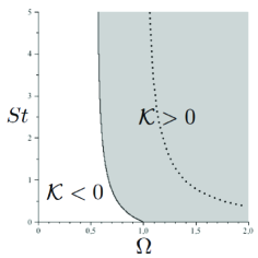
Figure 1: The sign of $\mathcal{K}$ in the $St-\Omega$ plane. Gray corresponds to $\mathcal{K}>0$; white to $\mathcal{K}<0$. The dotted line separates the region on its left, corresponding to transport enhancement due to inertia, from that on its right relative to transport reduction.

The presence of inertia thus causes a change of the sign of $\mathcal{K}$ from negative to positive in a subset of the $St-\Omega$ plane. In this region inertia thus plays to increase transport with respect to the tracer case. The region where transport is enhanced with respect to the tracer case actually extends up to the dotted line. To observe a reduction of transport, the Stokes time has thus to be sufficiently large. Larger and larger values are required for increasing $\Omega$.

The behavior of $\mathcal{K}$ as a function of $St$ is reported in Fig. 2 for different values of $\Omega$.

Figure 2: $\mathcal{K}$ vs St at $\Omega=0.2$ (upper panel), $\Omega=0.8$ (middle panel) and $\Omega=1.1$ (lower panel).

For sufficiently small $\Omega$, $\mathcal{K}$ is negative and inertia increases its value thus enhancing transport. For sufficiently large $\Omega$, $\mathcal{K}$ is positive and inertia increases its value up to a certain value of $St$ (corresponding to the intersection with the dotted line of Fig. 1) above which transport is reduced by inertia.

The physical explanation of the resulting behavior of $\mathcal{K}$ vs $St$, for small $St$, can be traced back to the mechanism of transport enhancement induced by a colored noise discussed in CaMa98 . Indeed, the random contribution to the inertial particle velocity in (8a) turns out to be a colored noise. The fact that for large Stokes times $\mathcal{K}$ goes to zero is a simple consequence of the fact that in such a limit the contribution of the noise to the particle trajectories becomes negligible because of the large inertia of the particles. A maximum of transport is thus guaranteed in all cases where $\mathcal{K}>0$ for $St=0$.

In conclusion, by explicit computation, we have shown that the eddy diffusivities of inertial particles can be determined for the class of shear flows for all values of the Stokes number. Although the analysis has been here confined on the sole case of heavy particles, following the same line of reasoning it is not difficult to show that the present results actually hold for any density ratio of the particles (i.e. for any value of the added-mass term $\beta$ involved in the model (2.2) of Ref. mamamu2012 ). We also show that the analytical results we obtained for the class of shear flows correspond to the leading order contribution either in the deviation from the shear flow geometry or in the Péclet number of general random Gaussian velocity fields (i.e. not of shear type).
The results we obtained for the eddy-diffusivity allowed us to investigate the role of inertia on the asymptotic transport regime. It turned out that both enhancement and reduction of transport (with respect to the tracer case) may occur depending on the extension of anticorrelated regions of the carrier flow Lagrangian auto-correlation function.

AM acknowledges with thanks the financial support from the PRIN 2012 project n. D38C13000610001 funded by the Italian Ministry of Education. We are also grateful for the financial support for the computational infrastructure from the Italian flagship project RITMARE.

References

(1)
IPCC: Fifth assessment report – the physical science basis, available at: http://www.ipcc.ch
(last access: 14 December 2015), (2013)
(2)
C. Denjean, F. Cassola, A. Mazzino, S. Triquet, S. Chevaillier, N.
Grand, T. Bourrianne, G. Momboisse, K. Sellegri, A. Schwarzenbock, E.
Freney, M. Mallet and P. Formenti,
Size distribution and optical properties of mineral dust aerosols
transported in the western Mediterranean.
Atmos. Chem. Phys.16, 1081-1104 (2016).
(3)
M. Martins Afonso,
The terminal velocity of sedimenting particles in a flowing fluid.
J. Phys. A: Math. Theor.41, 385501 (2008)
(4)
U. Frisch,
Lecture on turbulence and lattice gas hydrodynamics. In Lecture Notes,
NCAR- GTP Summer School June 1987 (ed. J. R. Herring & J. C.
McWilliams), 219-371. World Scientific. (1987)
(5)
U. Frisch, Turbulence. Cambridge Univ. Press. (1995)
(6)
M. Martins Afonso, A. Mazzino and P. Muratore-Ginanneschi,