What Is the True Value of Dynamic TDD:
A MAC Layer Perspective

Abstract

Small cell networks (SCNs) are envisioned to embrace dynamic time division duplexing (TDD) in order to tailor downlink (DL)/uplink (UL) subframe resources to quick variations and burstiness of DL/UL traffic. The study of dynamic TDD is particularly important because it provides valuable insights on the full duplex transmission technology, which has been identified as one of the candidate technologies for the 5th-generation (5G) networks. Up to now, the existing works on dynamic TDD have shown that the UL of dynamic TDD suffers from severe performance degradation due to the strong DL-to-UL interference in the physical (PHY) layer. This conclusion raises a fundamental question: Despite such obvious technology disadvantage, what is the true value of dynamic TDD? In this paper, we answer this question from a media access control (MAC) layer viewpoint and present analytical results on the DL/UL time resource utilization (TRU) of synchronous dynamic TDD, which has been widely adopted in the existing 4th-generation (4G) systems. Our analytical results shed new light on the dynamic TDD in future synchronous 5G networks.

I Introduction

An orthogonal deployment of dense small cell networks (SCNs) within the existing macrocell ones is characterized by small cells and macrocells operating on different frequency spectrum. Due to its capacity gain and easy implementation, such deployment is considered as one of the workhorses for capacity enhancement in the 4th-generation (4G) and 5th-generation (5G) networks, developed by the 3rd Generation Partnership Project (3GPP) [1, 2]. It is also envisaged that dense SCNs will embrace time division duplexing (TDD), which does not require a pair of frequency carriers, and offers the possibility of tailoring the amount of time radio resources to the downlink (DL)/uplink (UL) traffic conditions. In this line, seven TDD configurations, each associated with a specific DL/UL subframe number in a 10-milisecond TDD frame, are available for static or semi-static selection at the network side in the 4G Long Term Evolution (LTE) networks [3]. However, such static TDD operation cannot adapt DL/UL subframe resources to the fast fluctuations in DL/UL traffic demands.

To overcome the drawbacks of static TDD, a new technology, referred to as dynamic TDD, has recently drawn much attention [4, 5, 6, 7, 8]. In dynamic TDD, the configuration of the TDD DL/UL subframe number in each cell or a cluster of cells can be dynamically changed on a per-frame basis, i.e., once every 10 milliseconds [3]. Thus, dynamic TDD can provide a tailored configuration of DL/UL subframe resources for each cell or a cluster of cells at the expense of allowing inter-cell inter-link interference, e.g., DL transmissions of a cell may interfere with UL ones of a neighboring cell, and vice versa.

The study of dynamic TDD is particularly important because it provides valuable insights on the full duplex (FD) transmission [8, 9], which has been identified as one of the candidate technologies for 5G. In more detail,

• In an FD system, a base station (BS) can simultaneously transmit to and receive from different user equipments (UEs), thus enhancing spectrum reuse, but creating (i) inter-cell inter-link interference and (ii) intra-cell inter-link interference, a.k.a., self-interference [9].

• The main difference between an FD system and a dynamic TDD one is that intra-cell inter-link interference does not exist in dynamic TDD [8].

The physical (PHY) layer signal-to-interference-plus-noise ratio (SINR) performance of dynamic TDD has been analyzed in [4], assuming deterministic positions of BSs and UEs, and in [5, 6, 7], considering stochastic positions of BSs and UEs. The main conclusion in [4, 5, 6, 7] was that the UL SINR of dynamic TDD suffers from severe performance degradation due to the strong DL-to-UL interference, which is generated from a BS to another one. To address this challenge, cell clustering as well as full or partial interference cancellation (IC) at the BS side were recommended in [10, 11]. However, since clustering and IC are not trivial operations, such disadvantage of dynamic TDD in terms of UL SINR triggers a fundamental question: What is the true value of dynamic TDD? The answer can only be found through a thorough media access control (MAC) layer analysis, since the main motivation of dynamic TDD is to dynamically adapt DL/UL subframe resources to the variation of traffic demands. To the best our knowledge, the MAC layer analysis of dynamic TDD has not been investigated from a theoretical viewpoint in the literature, although some preliminary simulation results can be found in [8, 10, 11, 12].

In this paper, for the first time, we conduct a theoretical study on the MAC layer performance of dynamic TDD, and present a single contribution in this paper:

• We derive closed-form expressions of the DL/UL time resource utilization (TRU) for synchronous dynamic TDD, which has been widely adopted in the existing LTE systems. Such results quantify the performance of dynamic TDD in terms of its MAC layer resource usage, as SCNs evolve into dense and ultra-dense ones. More specifically,

  • We show that the DL/UL TRU varies across different TDD subframes.

  • We prove that the average total TRU of dynamic TDD is larger than that of static TDD.

  • We derive the limit of the performance gain of dynamic TDD compared with static TDD, in terms of the average total TRU.

II Network Scenario and Performance Metrics

In this section, we present the network scenario and the performance metrics considered in the paper.

II-A General Network Scenario

We consider a cellular network with BSs deployed on a plane according to a homogeneous Poisson point process (HPPP) $\Phi$ with a density of $\lambda$ $\textrm{BSs/km}^{2}$. Active UEs are also Poisson distributed in the considered network with a density of $\rho$ $\textrm{UEs/km}^{2}$. Here, we only consider active UEs in the network because non-active UEs do not trigger data transmissions.

In practice, a BS will mute its transmission, if there is no UE connected to it, which reduces inter-cell interference and energy consumption [13]. Note that such BS idle mode operation is not trivial, which even changes the capacity scaling law [14]. Since UEs are randomly and uniformly distributed in the network, we assume that the active BSs also follow an HPPP distribution $\tilde{\Phi}$ [15], the density of which is denoted by $\tilde{\lambda}$ $\textrm{BSs/km}^{2}$. Note that $0\leq\tilde{\lambda}\leq\lambda$, and a larger $\rho$ leads to a larger $\tilde{\lambda}$. From [15, 16], $\tilde{\lambda}$ is given by

$$\tilde{\lambda}=\lambda\left[1-\frac{1}{\left(1+\frac{\rho}{q\lambda}\right)^{q}}\right],$$ (1)

where $q$ takes an empirical value around 3.5~4 [15, 16].

For each active UE, the probabilities of it requesting DL and UL data are respectively denoted by $p^{{\rm{D}}}$ and $p^{{\rm{U}}}$, with $p^{{\rm{D}}}+p^{{\rm{U}}}=1$. Besides, we assume that each request is large enough to be transmitted for at least one TDD frame, which consists of $T$ subframes. In the sequel, the DL or UL subframe number per frame will be shortened as the DL or UL subframe number, because subframes are meant within one frame.

II-B Asynchronous and Synchronous Networks

Regarding TDD frames, we need to differentiate two types of networks, i.e., asynchronous ones and synchronous ones. Note that most previous works only investigated dynamic TDD operating in an asynchronous network [4, 5, 6, 7]. More specifically, in an asynchronous network, e.g., Wireless Fidelity (Wi-Fi), the TDD transmission frames are not aligned among cells, and thus both the PHY layer performance and the MAC layer one are uniform across all TDD subframes. However, in a synchronous network, such as LTE and the future 5G networks, the TDD transmission frames from different cells are aligned to simplify the design of the radio protocols. As a result, the performance of dynamic TDD becomes a function of the TDD configuration structure.

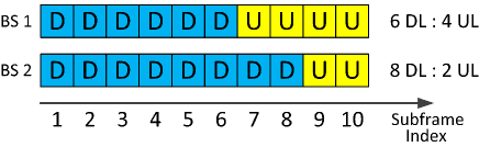
Fig. 1: An example of the LTE TDD configurations, where one TDD frame is composed of $T=10$ subframes. Here, ’D’ and ’U’ denote a DL subframe and an UL one, respectively.

Fig. 1 shows an example of such TDD configuration structure in LTE [3].

In Fig. 1, TDD frames of different cells are aligned in the time domain. One TDD frame is composed of $T=10$ subframes, and the time length of each subframe is 1 millisecond [3]. As an example, we assume that BS 1 and BS 2 use the TDD configurations with 6 and 8 DL subframes, respectively. For this synchronous network with TDD frame alignment, we have the following two remarks.

Remark 1: The first few subframes are more likely to carry DL transmissions than the last few ones. The opposite conclusion applies for the UL. This leads to a subframe dependent MAC layer performance of dynamic TDD.

Remark 2: The subframes in the middle of the frame are more likely to be subject to inter-cell inter-link interference than those at the two ends of the TDD frame. This implies a subframe dependent PHY layer performance of dynamic TDD.

Unfortunately, such synchronous dynamic TDD that has been used in LTE and will be used in 5G, has not been well treated in the literature, and previous works considering synchronous dynamic TDD were only based on simulations and lack of analytical rigor [8, 10, 11, 12]. In this paper, we explore Remark 1, and study the MAC layer performance of synchronous dynamic TDD, with the consideration of the DL-before-UL TDD configuration structure adopted in LTE, as illustrated in Fig. 1.

II-C MAC Layer Performance Metrics

For the $l$-th subframe ($l\in\left\{1,2,\ldots,T\right\}$), we define the subframe dependent DL TRU and UL TRU as the probability of BSs transmitting DL signals and that of UEs transmitting UL signals, respectively, which are denoted by $q_{l}^{{\rm{D}}}$ and $q_{l}^{{\rm{U}}}$. In other words, $q_{l}^{{\rm{D}}}$ and $q_{l}^{{\rm{U}}}$ characterize how much time resource is actually used for DL and UL, respectively. Note that generally we do not have $q_{l}^{{\rm{D}}}+q_{l}^{{\rm{U}}}=1$, because some subframe resources might be wasted, e.g., in static TDD.

Moreover, we define the average DL TRU $\kappa^{{\rm{D}}}$ and the average UL TRU $\kappa^{{\rm{U}}}$ as the mean value of $q_{l}^{{\rm{D}}}$ and $q_{l}^{{\rm{U}}}$ across all of the $T$ subframes:

$$\begin{cases}\begin{array}[]{l}\kappa^{{\rm{D}}}=\frac{1}{T}\sum_{l=1}^{T}q_{l}^{{\rm{D}}}\\ \kappa^{{\rm{U}}}=\frac{1}{T}\sum_{l=1}^{T}q_{l}^{{\rm{U}}}\end{array}\end{cases}.$$ (2)

Finally, we define the average total TRU $\kappa$ as the sum of $\kappa^{{\rm{D}}}$ and $\kappa^{{\rm{U}}}$, which is written as

$$\kappa=\kappa^{{\rm{D}}}+\kappa^{{\rm{U}}}.$$ (3)

In the following sections, we will investigate the performance of $q_{l}^{Link}$, $\kappa^{Link}$ and $\kappa$ considering Remark 1, where the string variable $Link$ denotes the link direction, and takes the value of ’D’ and ’U’ for the DL and the UL respectively.

III Main Results

The main goal of this section is to derive theoretical results on the DL/UL TRU defined in Subsection II-C. Note that computing $q_{l}^{{\rm{D}}}$ and $q_{l}^{{\rm{U}}}$ is a non-trivial task for synchronous dynamic TDD, because it involves the following distributions:

• the distribution of the UE number in an active BS, which will be shown to follow a truncated Negative Binomial distribution in Subsection III-A;

• the distribution of the DL/UL data request numbers in an active BS, which will be shown to follow a Binomial distribution in Subsection III-B;

• the dynamic TDD subframe splitting strategy and the corresponding distribution of the DL/UL subframe number, which will be shown to follow an aggregated Binomial distribution in Subsection III-C; and finally

• the prior information about the TDD frame structure, such as the DL-before-UL structure adopted in LTE [3] (see Fig. 1), which will lead to subframe dependent results of $q_{l}^{{\rm{D}}}$ and $q_{l}^{{\rm{U}}}$ to be presented in Subsection III-D.

III-A The Distribution of the UE Number in an Active BS: A Truncated Negative Binomial Distribution

According to [15], the coverage area size $X$ of a BS can be approximately characterized by a Gamma distribution [15], and its probability density function (PDF) is written as

$$f_{X}(x)=\left(q\lambda\right)^{q}x^{q-1}\frac{\exp(\text{\textminus}q\lambda x)}{\text{$\Gamma$}(q)},$$ (4)

where $\text{$\Gamma$}(\cdot)$ is the Gamma function [17]. Then, the UE number per BS can be denoted by a random variable (RV) $K$, and the probability mass function (PMF) of $K$ can be derived as

$$f_{K}\left(k\right) = \Pr\left[K=k\right]$$ (5)

$$\overset{\left(a\right)}{=} \int_{0}^{+\infty}\frac{\left(\rho x\right)^{k}}{k!}\exp(-\rho x)f_{X}(x)dx$$

$$\overset{\left(b\right)}{=} \frac{\Gamma(k+q)}{\Gamma(k+1)\Gamma(q)}\left(\frac{\rho}{\rho+q\lambda}\right)^{k}\left(\frac{q\lambda}{\rho+q\lambda}\right)^{q},$$

where $(a)$ is due to the HPPP distribution of UEs and $(b)$ is obtained from (4). It can be seen from (5) that $K$ follows a Negative Binomial distribution [17], i.e., $K\sim\textrm{NB}\left(q,\frac{\rho}{\rho+q\lambda}\right)$.

As discussed in Subsection II-A, we assume that a BS with $K=0$ is not active, which will be ignored in our analysis due to its muted transmission. Hence, we focus on the active BSs and further study the distribution of the UE number per active BS, which is denoted by a positive RV $\tilde{K}$. Considering (5) and the fact that the only difference between $K$ and $\tilde{K}$ lies in $\tilde{K}\neq 0$, we can conclude that $\tilde{K}$ follows a truncated Negative Binomial distribution, i.e., $\tilde{K}\sim\textrm{truncNB}\left(q,\frac{\rho}{\rho+q\lambda}\right)$. More specifically, the PMF of $\tilde{K}$ is denoted by $f_{\tilde{K}}\left(\tilde{k}\right),\tilde{k}\in\left\{1,2,\ldots,+\infty\right\}$, and it is given by

$$f_{\tilde{K}}\left(\tilde{k}\right)=\Pr\left[\tilde{K}=\tilde{k}\right]=\frac{f_{K}\left(\tilde{k}\right)}{1-f_{K}\left(0\right)},$$ (6)

where the denominator $\left(1-f_{K}\left(0\right)\right)$ represents the probability of a BS being active, i.e., $\tilde{\lambda}/\lambda$.

Example: As an example, we plot the results of $f_{\tilde{K}}\left(\tilde{k}\right)$ in Fig. 2 with the following parameter values: UE density $\rho=300\thinspace\textrm{UEs/km}^{2}$, BS density $\lambda\in\left\{50,200,1000\right\}\thinspace\textrm{BSs/km}^{2}$ and $q=4.05$ [13].

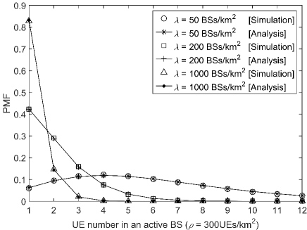
Fig. 2: The PMF of the UE number $\tilde{K}$ in an active BS ($\rho=300\thinspace\textrm{UEs/km}^{2}$, $q=4.05$, various $\lambda$).

From this figure, we can draw the following observations:

• The analytical results based on the truncated Negative Binomial distribution match well with the simulation results. More specifically, the maximum difference between the simulated PMF and the analytical PMF is shown to be less than 0.5 percentile.

• For the active BSs, $f_{\tilde{K}}\left(\tilde{k}\right)$ shows a more dominant peak at $\tilde{k}=1$ as $\lambda$, and in turn $\tilde{\lambda}$, increases. This is because the ratio of $\rho$ to $\tilde{\lambda}$ gradually decreases toward 1 as $\lambda$ increases, approaching the limit of one UE per active BS in ultra-dense SCNs. In particular, when $\lambda=1000\thinspace\textrm{BSs/km}^{2}$, more than 80 % of the active BSs will serve only one UE. Intuitively speaking, each of those BSs should dynamically engage all subframes for DL or UL transmissions based on the specific traffic demand of its served UE. In such way, the subframe resources can be fully utilized in dynamic TDD. Note that such operation is not available in static TDD due to its fixed TDD configuration.

III-B The Distribution of the DL/UL Data Request Number in an Active BS: A Binomial Distribution

After obtaining $f_{\tilde{K}}\left(\tilde{k}\right)$, we need to further study the distribution of the DL/UL data request number in an active BS, so that a tailored TDD configuration can be determined in a dynamic TDD network.

For clarity, the DL and UL data request numbers in an active BS are denoted by RVs $M^{{\rm{D}}}$ and $M^{{\rm{U}}}$, respectively. Since we assume that each UE generates one request of either DL data or UL data (see Subsection II-A), it is easy to show that

$$M^{{\rm{D}}}+M^{{\rm{U}}}=\tilde{K}.$$ (7)

As discussed in Subsection II-A, for each UE in an active BS, the probability of it requesting DL data and UL data is $p^{{\rm{D}}}$ and $p^{{\rm{U}}}$, respectively. Hence, for a given UE number $\tilde{k}$, $M^{{\rm{D}}}$ and $M^{{\rm{U}}}$ follow Binomial distributions [17], i.e., $M^{{\rm{D}}}\sim\textrm{Bi}\left(\tilde{k},p^{{\rm{D}}}\right)$ and $M^{{\rm{U}}}\sim\textrm{Bi}\left(\tilde{k},p^{{\rm{U}}}\right)$. More specifically, the PMFs of $M^{{\rm{D}}}$ and $M^{{\rm{U}}}$ can be respectively written as

$$f_{M^{{\rm{D}}}}\left(m^{{\rm{D}}}\right) = \left(\begin{array}[]{c}\tilde{k}\\ m^{{\rm{D}}}\end{array}\right)\left(p^{{\rm{D}}}\right)^{m^{{\rm{D}}}}\left(1-p^{{\rm{D}}}\right)^{\tilde{k}-m^{{\rm{D}}}},$$ (10)

and

$$f_{M^{{\rm{U}}}}\left(m^{{\rm{U}}}\right) = \left(\begin{array}[]{c}\tilde{k}\\ m^{{\rm{U}}}\end{array}\right)\left(p^{{\rm{U}}}\right)^{m^{{\rm{U}}}}\left(1-p^{{\rm{U}}}\right)^{\tilde{k}-m^{{\rm{U}}}}.$$ (13)

Example: As an example, we plot the results of $f_{M^{{\rm{D}}}}\left(m^{{\rm{D}}}\right)$ in Fig. 3 with the following parameter values: $p^{{\rm{D}}}=\frac{2}{3}$ and $\tilde{k}\in\left\{1,4,12\right\}$. For brevity, we omit displaying the PMF of $M^{{\rm{U}}}$, due to its duality to $M^{{\rm{D}}}$ as shown in (7).

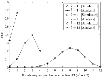
Fig. 3: The PMF of the DL data request number $M^{{\rm{D}}}$ in an active BS ($p^{{\rm{D}}}=\frac{2}{3}$, various $\tilde{k}$).

From this figure, we can draw the following observations:

• The Binomial distribution accurately characterizes the distribution of $M^{{\rm{D}}}$, as the analytical PMFs well match the simulated ones.

• The average value of $M^{{\rm{D}}}$ is around $p^{{\rm{D}}}\tilde{k}$, which is inline with intuition.

III-C The Distribution of the DL/UL Subframe Number with Dynamic TDD: An Aggregated Binomial Distribution

After knowing the distribution of the DL data request number $M^{{\rm{D}}}$ in an active BS, we are now ready to consider dynamic TDD, and derive the distribution of the DL subframe number in an active BS. For a given UE number $\tilde{k}$, the DL subframe number in an active BS is denoted by $N^{{\rm{D}}}$. Here, we adopt a dynamic TDD algorithm to choose the DL subframe number, which matches the DL subframe ratio with the DL data request ratio [8]. In more detail, for certain values of $m^{{\rm{D}}}$ and $\tilde{k}$, the DL subframe number $n\left(m^{{\rm{D}}},\tilde{k}\right)$ is determined by

$$n\left(m^{{\rm{D}}},\tilde{k}\right)=\textrm{round}\left(\frac{m^{{\rm{D}}}}{\tilde{k}}T\right),$$ (14)

where $\textrm{round}\left(x\right)$ is an operator that rounds a real value $x$ to its nearest integer. In (14), $\frac{m^{{\rm{D}}}}{\tilde{k}}$ can be deemed as the DL data request ratio, because (i) $m^{{\rm{D}}}$ denotes the DL data request number with its distribution characterized in (10); and (ii) $\tilde{k}$ represents the UE number, and thus the total number of the DL and UL data requests. As a result, $\frac{m^{{\rm{D}}}}{\tilde{k}}T$ yields the desirable DL subframe number that matches the DL subframe ratio with the DL data request ratio. Due to the integer nature of the DL subframe number, we use the round operator to generate a valid DL subframe number that is nearest to $\frac{m^{{\rm{D}}}}{\tilde{k}}T$ in (14).

Based on (14), the PMF of $N^{{\rm{D}}}$ is denoted by $f_{N^{{\rm{D}}}}\left(n^{{\rm{D}}}\right),n^{{\rm{D}}}\in\left\{0,1,\ldots,T\right\}$, and it can be derived as

$$f_{N^{{\rm{D}}}}\left(n^{{\rm{D}}}\right) = \Pr\left[N^{{\rm{D}}}=n^{{\rm{D}}}\right]$$ (15)

$$\overset{\left(a\right)}{=} \sum_{m^{{\rm{D}}}=0}^{\tilde{k}}I\left\{\textrm{round}\left(\frac{m^{{\rm{D}}}}{\tilde{k}}T\right)=n^{{\rm{D}}}\right\}f_{M^{{\rm{D}}}}\left(m^{{\rm{D}}}\right),$$

where (14) is plugged into (a), and $I\left\{X\right\}$ is an indicator function that outputs one when $X$ is true and zero otherwise. Besides, $f_{M^{{\rm{D}}}}\left(m^{{\rm{D}}}\right)$ is computed by (10). Due to the existence of the indicator function in (15), $f_{N^{{\rm{D}}}}\left(n^{{\rm{D}}}\right)$ can be viewed as an aggregated PMF of Binomial PMFs, since $N^{{\rm{D}}}$ is computed from $M^{{\rm{D}}}$ according to a many-to-one mapping in (14).

Because the total subframe number in a frame is $T$, and each subframe should be either a DL one or an UL one, it is apparent that $N^{{\rm{D}}}+N^{{\rm{U}}}=T$, and thus we have

$$f_{N^{{\rm{U}}}}\left(n^{{\rm{U}}}\right)=f_{N^{{\rm{D}}}}\left(T-n^{{\rm{U}}}\right).$$ (16)

Example: As an example, we plot the results of $f_{N^{{\rm{D}}}}\left(n^{{\rm{D}}}\right)$ in Fig. 4 with the following parameter values: $p^{{\rm{D}}}=\frac{2}{3}$, $T=10$ and $\tilde{k}\in\left\{1,4,12\right\}$.

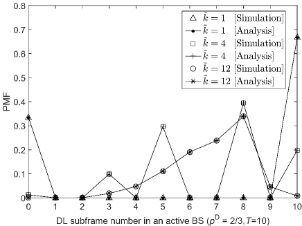
Fig. 4: The PMF of the DL subframe number $N^{{\rm{D}}}$ in an active BS ($p^{{\rm{D}}}=\frac{2}{3}$, $T=10$, various $\tilde{k}$).

From this figure, we can draw the following observations:

• Following the logic of dynamic TDD characterized in (14), when $\tilde{k}=1$, the DL subframe number is set to either $T=10$ or 0, meaning that the active BS dynamically invest all subframes in DL transmissions or UL transmissions based on the instantaneous data request being DL (with a probability of $p^{{\rm{D}}}$) or UL (with a probability of $p^{{\rm{U}}}$). Such strategy fully utilizes the subframe resources in a dynamic TDD network.

• When $\tilde{k}>1$, the PMF of the DL subframe number turns out to be rather complex, because multiple DL data request numbers may be mapped to the same DL subframe number due to the dynamic TDD algorithm given by (14). For example, when $\tilde{k}=12$, we have $f_{N^{{\rm{D}}}}\left(8\right)=0.339$ as exhibited in Fig. 4. This is because:

  • according to (14), both $M^{{\rm{D}}}=9$ and $M^{{\rm{D}}}=10$ result in $N^{{\rm{D}}}=8$, since $\textrm{round}\left(\frac{9}{12}\times 10\right)=8$ and $\textrm{round}\left(\frac{10}{12}\times 10\right)=8$. In other words, with dynamic TDD, 8 subframes will be allocated for the DL, if either 9 or 10 data requests in $\tilde{k}=12$ data requests are DL;

  • as shown in Fig. 3, $f_{M^{{\rm{D}}}}\left(9\right)=0.212$ and $f_{M^{{\rm{D}}}}\left(10\right)=0.127$; and thus

  • from (15), we have $f_{N^{{\rm{D}}}}\left(8\right)=f_{M^{{\rm{D}}}}\left(9\right)+f_{M^{{\rm{D}}}}\left(10\right)=0.339$. In other words, with dynamic TDD, the probability of allocating 8 DL subframes equals to the sum of the probabilities of observing 9 and 10 DL data requests in 12 data requests.

III-D The Subframe Dependent DL/UL TRU

In this subsection, we present our main results on the subframe dependent DL/UL TRUs $q_{l}^{{\rm{D}}}$ and $q_{l}^{{\rm{U}}}$ for dynamic TDD in Theorem 1.

Theorem 1.

For dynamic TDD, $q_{l}^{{\rm{D}}}$ and $q_{l}^{{\rm{U}}}$ are given by

$$\begin{cases}\begin{array}[]{l}q_{l}^{{\rm{D}}}=\sum_{\tilde{k}=1}^{+\infty}\left(1-\sum_{i=0}^{l-1}f_{N^{{\rm{D}}}}\left(i\right)\right)f_{\tilde{K}}\left(\tilde{k}\right)\\ q_{l}^{{\rm{U}}}=\sum_{\tilde{k}=1}^{+\infty}\sum_{i=0}^{l-1}f_{N^{{\rm{D}}}}\left(i\right)f_{\tilde{K}}\left(\tilde{k}\right)\end{array}\end{cases},$$ (17)

where $f_{N^{{\rm{D}}}}\left(i\right)$ and $f_{\tilde{K}}\left(\tilde{k}\right)$ are given by (15) and (6), respectively.

Proof:

Based on (15) and conditioned on $\tilde{K}=\tilde{k}$, the probability of performing a DL transmission in subframe $l$ $\left(l\in\left\{1,2,\ldots,T\right\}\right)$ can be calculated as

$$q_{l,\tilde{k}}^{{\rm{D}}} = \Pr\left[\left.Y_{l}={\rm{\textrm{'}D\textrm{'}}}\right|\tilde{K}=\tilde{k}\right]$$ (18)

$$\overset{\left(a\right)}{=} \Pr\left[N^{{\rm{D}}}\geq l\right]$$

$$= 1-F_{N^{{\rm{D}}}}\left(l-1\right),$$

where $Y_{l}$ denotes the link direction for the transmission on the $l$-th subframe, which takes a string value of ’D’ and ’U’ for the DL and the UL, respectively. Besides, the step $(a)$ of (18) is due to the LTE TDD configuration structure shown in Fig. 1, and $F_{N^{{\rm{D}}}}\left(n^{{\rm{D}}}\right)$ is the cumulative mass function (CMF) of $N^{{\rm{D}}}$ in an active BS, which is written as

$$F_{N^{{\rm{D}}}}\left(n^{{\rm{D}}}\right)=\Pr\left[N^{{\rm{D}}}\leq n^{{\rm{D}}}\right]=\sum_{i=0}^{n^{{\rm{D}}}}f_{N^{{\rm{D}}}}\left(i\right).$$ (19)

Considering the dynamic allocation of subframe to the DL and the UL in dynamic TDD, the conditional probability of performing an UL transmission in subframe $l$ is given by

$$q_{l,\tilde{k}}^{{\rm{U}}}=1-q_{l,\tilde{k}}^{{\rm{D}}}=F_{N^{{\rm{D}}}}\left(l-1\right).$$ (20)

Furthermore, the unconditional probabilities of performing a DL and UL transmissions on the $l$-th subframe, i.e., $q_{l}^{{\rm{D}}}$ and $q_{l}^{{\rm{U}}}$, can be respectively derived by calculating the expected values of $q_{l,\tilde{k}}^{{\rm{D}}}$ and $q_{l,\tilde{k}}^{{\rm{U}}}$ over all the possible values of $\tilde{k}$ as shown in (17), which concludes our proof. ∎

III-E The Average DL/UL/Total TRU

From Theorem 1, and Equations (2) and (3), we can obtain the results on the average DL/UL/total TRU for dynamic TDD, which are summarized in Lemma 2.

Lemma 2.

For dynamic TDD, $\left\{\kappa^{{\rm{D}}},\kappa^{{\rm{U}}},\kappa\right\}$ is given by

$$\begin{cases}\begin{array}[]{l}\kappa^{{\rm{D}}}=\frac{1}{T}\sum_{l=1}^{T}\sum_{\tilde{k}=1}^{+\infty}\left(1-\sum_{i=0}^{l-1}f_{N^{{\rm{D}}}}\left(i\right)\right)f_{\tilde{K}}\left(\tilde{k}\right)\\ \kappa^{{\rm{U}}}=\frac{1}{T}\sum_{l=1}^{T}\sum_{\tilde{k}=1}^{+\infty}\sum_{i=0}^{l-1}f_{N^{{\rm{D}}}}\left(i\right)f_{\tilde{K}}\left(\tilde{k}\right)\\ \kappa=1\end{array}\end{cases},$$ (21)

where $f_{N^{{\rm{D}}}}\left(i\right)$ and $f_{\tilde{K}}\left(\tilde{k}\right)$ are given by (15) and (6), respectively.

Proof:

The proof is straightforward by plugging (17) into (2) and (3). ∎

Lemma 2 not only quantifies the average MAC layer performance of dynamic TDD, but also shows from a theoretical viewpoint that dynamic TDD always achieves a full resource utilization, i.e., $\kappa=1$, thanks to the smart adaption of DL/UL subframes to DL/UL data requests.

Next, we present our main results on $\kappa^{{\rm{D}}}$, $\kappa^{{\rm{U}}}$ and $\kappa$ for static TDD in Theorem 3.

Theorem 3.

For static TDD, $\left\{\kappa^{{\rm{D}}},\kappa^{{\rm{U}}},\kappa\right\}$ can be derived as

$$\begin{cases}\begin{array}[]{l}\kappa^{{\rm{D}}}=\left(1-\sum_{\tilde{k}=1}^{+\infty}\left(1-p^{{\rm{D}}}\right)^{\tilde{k}}f_{\tilde{K}}\left(\tilde{k}\right)\right)\frac{N_{0}^{{\rm{D}}}}{T}\\ \kappa^{{\rm{U}}}=\left(1-\sum_{\tilde{k}=1}^{+\infty}\left(1-p^{{\rm{U}}}\right)^{\tilde{k}}f_{\tilde{K}}\left(\tilde{k}\right)\right)\frac{N_{0}^{{\rm{U}}}}{T}\\ \kappa=\frac{1}{T}\sum_{\tilde{k}=1}^{+\infty}\left[\left(1-\left(p^{{\rm{U}}}\right)^{\tilde{k}}\right)N_{0}^{{\rm{D}}}+\left(1-\left(p^{{\rm{D}}}\right)^{\tilde{k}}\right)N_{0}^{{\rm{U}}}\right]f_{\tilde{K}}\left(\tilde{k}\right)\end{array}\end{cases},$$ (22)

where $f_{\tilde{K}}\left(\tilde{k}\right)$ is obtained from (6), and $N_{0}^{{\rm{D}}}$ and $N_{0}^{{\rm{U}}}$ are the designated subframe numbers for the DL and the UL in static TDD, respectively, which satisfy $N_{0}^{{\rm{D}}}+N_{0}^{{\rm{U}}}=T$.

Proof:

In static TDD, for a given UE number $\tilde{k}$ in an active BS, the probabilities that no UE requests any DL data and no UE requests any UL data can be calculated by $f_{M^{{\rm{D}}}}\left(0\right)$ from (10) and $f_{M^{{\rm{U}}}}\left(0\right)$ from (13), respectively. Even in such cases, static TDD still unwisely allocates $N_{0}^{{\rm{D}}}$ and $N_{0}^{{\rm{U}}}$ subframes for the DL and the UL, respectively, which causes resource waste. The probabilities of such resource waste for the DL and the UL are denoted by $w^{{\rm{D}}}$ and $w^{{\rm{U}}}$, and they can be calculated as

$$\begin{cases}\begin{array}[]{l}w^{{\rm{D}}}=\sum_{\tilde{k}=1}^{+\infty}f_{M^{{\rm{D}}}}\left(0\right)f_{\tilde{K}}\left(\tilde{k}\right)=\sum_{\tilde{k}=1}^{+\infty}\left(1-p^{{\rm{D}}}\right)^{\tilde{k}}f_{\tilde{K}}\left(\tilde{k}\right)\\ w^{{\rm{U}}}=\sum_{\tilde{k}=1}^{+\infty}f_{M^{{\rm{U}}}}\left(0\right)f_{\tilde{K}}\left(\tilde{k}\right)=\sum_{\tilde{k}=1}^{+\infty}\left(1-p^{{\rm{U}}}\right)^{\tilde{k}}f_{\tilde{K}}\left(\tilde{k}\right)\end{array}\end{cases}.$$ (23)

Excluding such resource waste from $N_{0}^{{\rm{D}}}$ and $N_{0}^{{\rm{U}}}$, we can obtain $\kappa^{{\rm{D}}}$ and $\kappa^{{\rm{U}}}$ for static TDD as

$$\begin{cases}\begin{array}[]{l}\kappa^{{\rm{D}}}=\left(1-w^{{\rm{D}}}\right)\frac{N_{0}^{{\rm{D}}}}{T}\\ \kappa^{{\rm{U}}}=\left(1-w^{{\rm{U}}}\right)\frac{N_{0}^{{\rm{U}}}}{T}\end{array}\end{cases}.$$ (24)

Our proof is thus completed by plugging (23), (10) and (13) into (24), followed by computing $\kappa$ from (3). ∎

From Lemma 2 and Theorem 3, we can further quantify the additional total TRU achieved by dynamic TDD as

$$\kappa^{{\rm{ADD}}}=\frac{1}{T}\sum_{\tilde{k}=1}^{+\infty}\left[\left(p^{{\rm{U}}}\right)^{\tilde{k}}N_{0}^{{\rm{D}}}+\left(p^{{\rm{D}}}\right)^{\tilde{k}}N_{0}^{{\rm{U}}}\right]f_{\tilde{K}}\left(\tilde{k}\right),$$ (25)

where $\kappa^{{\rm{ADD}}}$ measures the difference of $\kappa$ in (21) and that in (22).

In addition, we present the performance limit of $\kappa^{{\rm{ADD}}}$ in Lemma 4.

Lemma 4.

When $\lambda\rightarrow+\infty$, the limit of $\kappa^{{\rm{ADD}}}$ is given by

$$\underset{\lambda\rightarrow+\infty}{\lim}\kappa^{{\rm{ADD}}}=\frac{p^{{\rm{D}}}N_{0}^{{\rm{U}}}}{T}+\frac{p^{{\rm{U}}}N_{0}^{{\rm{D}}}}{T}.$$ (26)

Proof:

From (6), we have $\underset{\lambda\rightarrow+\infty}{\lim}\Pr\left[\tilde{K}=1\right]=1$. Hence, using Lemma 2, we can draw the following conclusion for dynamic TDD:

$$\begin{cases}\begin{array}[]{l}\underset{\lambda\rightarrow+\infty}{\lim}\kappa^{{\rm{D}}}=1-f_{N^{{\rm{D}}}}\left(0\right)=1-p^{{\rm{U}}}=p^{{\rm{D}}}\\ \underset{\lambda\rightarrow+\infty}{\lim}\kappa^{{\rm{U}}}=1-f_{N^{{\rm{U}}}}\left(0\right)=1-p^{{\rm{D}}}=p^{{\rm{U}}}\end{array}\end{cases}.$$ (27)

Based on $\underset{\lambda\rightarrow+\infty}{\lim}\Pr\left[\tilde{K}=1\right]=1$ and Theorem 3, we can obtain the following conclusion for static TDD:

$$\begin{cases}\begin{array}[]{l}\underset{\lambda\rightarrow+\infty}{\lim}\kappa^{{\rm{D}}}=\left(1-\left(1-p^{{\rm{D}}}\right)\right)\frac{N_{0}^{{\rm{D}}}}{T}=\frac{p^{{\rm{D}}}N_{0}^{{\rm{D}}}}{T}\\ \underset{\lambda\rightarrow+\infty}{\lim}\kappa^{{\rm{U}}}=\left(1-\left(1-p^{{\rm{U}}}\right)\right)\frac{N_{0}^{{\rm{U}}}}{T}=\frac{p^{{\rm{U}}}N_{0}^{{\rm{U}}}}{T}\end{array}\end{cases}.$$ (28)

Our proof is completed by comparing (27) with (28). ∎

Note that in (26) of Lemma 4, the first and the second terms are contributed from the DL and the UL, respectively.

IV Simulation and Discussion

In this section, we present numerical results to validate the accuracy of our analysis. In our simulations, the UE density is set to $\rho=300\thinspace\textrm{UEs/km}^{2}$, which leads to $q=4.05$ in (4) [13]. In addition, we assume that $p^{{\rm{D}}}=\frac{2}{3}$ and $T=10$. Thus, for static TDD, we have $N_{0}^{{\rm{D}}}=7$ and $N_{0}^{{\rm{U}}}=3$ in (22), which achieves the best match with $p^{{\rm{D}}}$ and $p^{{\rm{U}}}$, according to (14).

IV-A Validation of the Results on the Subframe Dependent TRU

In Fig. 5, we plot the analytical and simulation results of $q_{l}^{{\rm{D}}}$.

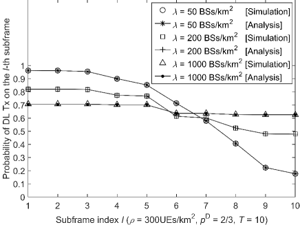
Fig. 5: The subframe dependent DL TRU $q_{l}^{{\rm{D}}}$.

For brevity, we omit showing the results of $q_{l}^{{\rm{U}}}$, due to its duality to $q_{l}^{{\rm{D}}}$ as shown in (20).

From this figure, we can see that:

• The analytical results of $q_{l}^{{\rm{D}}}$ match well with the simulation results. More specifically, the maximum difference between the simulation results and the analytical results is shown to be less than 0.3 %. Note that the curves are not smooth in Fig. 5. This is because of the non-continuous mapping in (14), not due to an insufficient number of simulation experiments.

• $q_{l}^{{\rm{D}}}$ monotonically decreases with $l$ because of the considered DL-before-UL TDD configuration structure shown in Fig. 1. In other words, DL transmissions, if scheduled by BSs, are likely to be conducted in earlier subframes.

• When $\lambda$ is relatively small compared with $\rho$, e.g., $\lambda=50\thinspace\textrm{BSs/km}^{2}$, $q_{1}^{{\rm{D}}}$ is almost one and $q_{10}^{{\rm{D}}}$ is close to zero. This is because:

  • the UE number in an active BS tends to be relatively large, e.g., the typical value of $\tilde{k}$ is around $4\thinspace\textrm{UEs/BS}$ when $\lambda=50\thinspace\textrm{BSs/km}^{2}$, as exhibited in Fig. 2;

  • as a result, the DL data request number is non-zero for most cases, e.g., around $m^{{\rm{D}}}=3\thinspace$DL data requests when $p^{{\rm{D}}}=\frac{2}{3}$ and $\tilde{k}=4$, as shown in Fig. 3;

  • thus, the DL subframe number is also relatively large to accommodate those DL data requests, e.g., the typical value of $n^{{\rm{D}}}$ is $\left\{3,5,8\right\}$ DL subframes when $p^{{\rm{D}}}=\frac{2}{3}$, $\tilde{k}=4$ and $T=10$; as displayed in Fig. 4;

  • due to the DL-before-UL LTE TDD configuration structure shown in Fig. 1, the first subframe has a very high probability to be a DL one, i.e., $q_{1}^{{\rm{D}}}$ is almost one, and the last subframe is the most likely not to be a DL one, i.e., $q_{10}^{{\rm{D}}}$ is close to zero.

• When $\lambda$ is relatively large compared with $\rho$, e.g., $\lambda=1000\thinspace\textrm{BSs/km}^{2}$, $q_{l}^{{\rm{D}}}$ is nearly a constant for all values of $l$. Such constant roughly equals to the DL data request probability $p^{{\rm{D}}}=\frac{2}{3}$. This is because:

  • more than 80 % of the active BSs will serve $\tilde{k}=1$ UE when $\lambda=1000\thinspace\textrm{BSs/km}^{2}$, as exhibited in Fig. 2;

  • as a result, when $\tilde{k}=1$, both the DL data request number and the DL subframe number show high fluctuation, as illustrated in Figs. 3 and 4 due to the strong traffic dynamics;

  • and hence, in most cases, all the subframes are used as either DL ones or UL ones, the probability of which depends on the DL or UL data request probability. Since $p^{{\rm{D}}}=\frac{2}{3}$, we have that $q_{l}^{{\rm{D}}}\approx\frac{2}{3}$.

• It is straightforward to see that the case of $\lambda=200\thinspace\textrm{BSs/km}^{2}$ plays in the middle of the above two cases.

IV-B Validation of the Results on the Average TRU

In Fig. 6, we display the analytical and simulation results of $\kappa^{{\rm{D}}}$ and $\kappa^{{\rm{U}}}$.

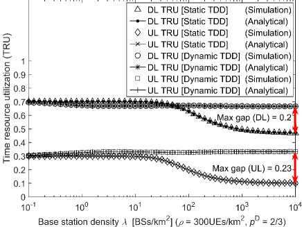
Fig. 6: The average DL/UL TRU $\kappa^{{\rm{D}}}$ and $\kappa^{{\rm{U}}}$.

From this figure, we can see that:

• The analytical results of $\kappa^{{\rm{D}}}$ and $\kappa^{{\rm{U}}}$ match well with the simulation results for both static TDD and dynamic TDD.

• The sum of $\kappa^{{\rm{D}}}$ and $\kappa^{{\rm{U}}}$, i.e., $\kappa$, for dynamic TDD is shown to always equal to one, which verifies Lemma 2, and shows the main advantage of dynamic TDD.

• The $\kappa$ for static TDD become smaller than one in dense SCNs, e.g., $\lambda>10\thinspace\textrm{BSs/km}^{2}$, which verifies Theorem 3, and shows the main drawback of static TDD.

• According to Lemma 4, the additional total TRU achievable by dynamic TDD, $\underset{\lambda\rightarrow+\infty}{\lim}\kappa^{{\rm{ADD}}}$, should be composed of two parts, i.e., one from the DL ($\frac{p^{{\rm{D}}}N_{0}^{{\rm{U}}}}{T}$) and another one from the UL ($\frac{p^{{\rm{U}}}N_{0}^{{\rm{D}}}}{T}$), which in this case are 0.2 and 0.23, respectively. These values can be validated in Fig. 6. Thus, the average total gain of dynamic TDD over static TDD in terms of $\underset{\lambda\rightarrow+\infty}{\lim}\kappa^{{\rm{ADD}}}$ is 0.43 (+$75.4\,\%$).

V Conclusion

For the first time, we investigated the MAC layer TRU for synchronous dynamic TDD with the network densification, which quantifies the performance of dynamic TDD in terms of its MAC layer resource usage. We showed that the DL/UL TRU varies across TDD subframes, and that dynamic TDD can achieve an increasingly higher average total TRU than static TDD with the network densification of up to $75.4\,\%$. As future work, we will combined our results on the MAC layer TRU with the PHY layer SINR results to derive the total area spectral efficiency for synchronous dynamic TDD.

References

- [1] D. L pez-P rez, M. Ding, H. Claussen, and A. Jafari, “Towards 1 Gbps/UE in cellular systems: Understanding ultra-dense small cell deployments,” IEEE Communications Surveys Tutorials, vol. 17, no. 4, pp. 2078–2101, Jun. 2015.
- [2] X. Ge, S. Tu, G. Mao, C. X. Wang, and T. Han, “5G ultra-dense cellular networks,” IEEE Wireless Communications, vol. 23, no. 1, pp. 72–79, Feb. 2016.
- [3] 3GPP, “TR 36.828: Further enhancements to LTE Time Division Duplex for Downlink-Uplink interference management and traffic adaptation,” Jun. 2012.
- [4] M. Ding, D. L pez-P rez, A. V. Vasilakos, and W. Chen, “Analysis on the SINR performance of dynamic TDD in homogeneous small cell networks,” 2014 IEEE Global Communications Conference, pp. 1552–1558, Dec. 2014.
- [5] H. Sun, M. Wildemeersch, M. Sheng, and T. Q. S. Quek, “D2d enhanced heterogeneous cellular networks with dynamic tdd,” IEEE Transactions on Wireless Communications, vol. 14, no. 8, pp. 4204–4218, Aug. 2015.
- [6] B. Yu, L. Yang, H. Ishii, and S. Mukherjee, “Dynamic TDD support in macrocell-assisted small cell architecture,” IEEE Journal on Selected Areas in Communications, vol. 33, no. 6, pp. 1201–1213, Jun. 2015.
- [7] A. K. Gupta, M. N. Kulkarni, E. Visotsky, F. W. Vook, A. Ghosh, J. G. Andrews, and R. W. Heath, “Rate analysis and feasibility of dynamic TDD in 5G cellular systems,” 2016 IEEE International Conference on Communications (ICC), pp. 1–6, May 2016.
- [8] M. Ding, D. L pez-P rez, R. Xue, A. Vasilakos, and W. Chen, “On dynamic Time-Division-Duplex transmissions for small-cell networks,” IEEE Transactions on Vehicular Technology, vol. 65, no. 11, pp. 8933–8951, Nov. 2016.
- [9] S. Goyal, C. Galiotto, N. Marchetti, and S. Panwar, “Throughput and coverage for a mixed full and half duplex small cell network,” IEEE International Conference on Communications (ICC), pp. 1–7, May 2016.
- [10] M. Ding, D. L pez-P rez, A. V. Vasilakos, and W. Chen, “Dynamic TDD transmissions in homogeneous small cell networks,” 2014 IEEE International Conference on Communications Workshops (ICC), pp. 616–621, Jun. 2014.
- [11] M. Ding, D. L pez-P rez, R. Xue, A. V. Vasilakos, and W. Chen, “Small cell dynamic tdd transmissions in heterogeneous networks,” 2014 IEEE International Conference on Communications (ICC), pp. 4881–4887, Jun. 2014.
- [12] Z. Shen, A. Khoryaev, E. Eriksson, and X. Pan, “Dynamic uplink-downlink configuration and interference management in td-lte,” IEEE Communications Magazine, vol. 50, no. 11, pp. 51–59, Nov. 2012.
- [13] M. Ding, D. L pez-P rez, G. Mao, and Z. Lin, “Performance impact of idle mode capability on dense small cell networks with LoS and NLoS transmissions,” arXiv:1609.07710 [cs.NI], Sep. 2016.
- [14] M. Ding, D. L pez-P rez, and G. Mao, “A new capacity scaling law in ultra-dense networks,” arXiv:1704.00399 [cs.NI], Apr. 2017. [Online]. Available: https://arxiv.org/abs/1704.00399
- [15] S. Lee and K. Huang, “Coverage and economy of cellular networks with many base stations,” IEEE Communications Letters, vol. 16, no. 7, pp. 1038–1040, Jul. 2012.
- [16] M. Ding, D. L pez-P rez, G. Mao, and Z. Lin, “Study on the idle mode capability with LoS and NLoS transmissions,” IEEE Globecom 2016, pp. 1–6, Dec. 2016.
- [17] I. Gradshteyn and I. Ryzhik, Table of Integrals, Series, and Products (7th Ed.). Academic Press, 2007.