Error-detected generation and complete analysis of hyperentangled Bell states for photons assisted by quantum-dot spins in double-sided optical microcavities

Abstract

We construct an error-detected block, assisted by the quantum-dot spins in double-sided optical microcavities. With this block, we propose three error-detected schemes for the deterministic generation, the complete analysis, and the complete nondestructive analysis of hyperentangled Bell states in both the polarization and spatial-mode degrees of freedom of two-photon systems. In these schemes, the errors can be detected, which can improve their fidelities largely, far different from other previous schemes assisted by the interaction between the photon and the quantum-dot-cavity system. Our scheme for the deterministic generation of hyperentangled two-photon systems can be performed by repeat until success. These features make our schemes more useful in high-capacity quantum communication with hyperentanglement in the future.

I Introduction

Quantum entanglement plays a critical role in quantum information processing quantum1 and it is a key quantum resource in quantum communication, such as quantum teleportation tele1 , quantum dense coding dense1 ; super2 , quantum key distribution Ekert , quantum secret sharing QSS1 , quantum secure direct communication QSDC1 ; twostep , and so on. The complete and deterministic analysis of Bell states is required to achieve some important tasks in quantum communication. In 1999, two schemes of Bell-state analysis (BSA) BSA1 ; BSA2 for teleportation with only linear optical elements were proposed. However, it is impossible to deterministically and completely distinguish the four Bell states in polarization with only linear optical elements BSA3 ; BSA4 ; BSA5 . In 2005, Barrett et al. BSA9 proposed an analyzer for distinguishing all four polarization Bell states using weak nonlinearities. In 2015, Sheng et al. LBSA realized the near complete logic Bell-state analysis by using the cross-Kerr nonlinearity. The complete BSA can be accomplished with the assistance of hyperentanglement BSA7 ; BSA8 ; hyper9 ; hyper8 ; DEPPTS . In 1998, Kwiat and Weinfurter BSA7 introduced the method to distinguish the four Bell states of photon pairs in the polarization degree of freedom (DOF) with the assistance of the hyperentanglement in both the polarization DOF and the momentum DOF. In 2003, Walborn et al. BSA8 proposed a simple linear-optical scheme for the complete Bell-state measurement of photons by using hyperentangled states with linear optics. In 2006, Schuck et al. hyper9 deterministically distinguished polarization Bell states of entangled photon pairs completely assisted by polarization-time-bin hyperentangled states in experiment. In 2007, Barbieri et al. hyper8 realized a complete and deterministic Bell-state measurement using linear optics and two-photon hyperentangled in polarization and momentum DOFs in experiment.

Besides the assistance for the complete BSA, hyperentanglement, a state of a quantum system being simultaneously entangled in multiple DOFs, has attracted much attention as it can improve the channel capacity largely, beat the channel capacity of linear photonic superdense coding super1 , and can be used for quantum error-correcting code correct and quantum repeaters repeater2 . Some theoretical and experimental schemes for the generation of hyperentangled states have been proposed and implemented in optical systems hyper1 ; hyper2 ; hyper3 ; hyper4 ; hyper5 ; hyper6 , such as polarization-momentum DOFs hyper2 , polarization-orbital-angular momentum DOFs hyper4 , multipath DOFs hyper5 , and so on. In 2009, Vallone et al. hyper6 demonstrated experimentally the generation of a two-photon six-qubit hyperentangled state in three DOFs. A hyperentangled photon pair, which is hyperentangled in both the polarization and spatial-mode DOFs with $16$ orthogonal Bell states, can be produced by spontaneous parametric down-conversion source with the $\beta$ barium borate crystal. However the quantum efficiency of this method is low and the the multiphoton generation probability is high, which will limit the application of hyperentanglement in quantum information processing. Moreover, one cannot distinguish the $16$ Bell states completely with only linear optics. In 2010, Sheng et al. HBSA1 proposed the first scheme for the complete hyperentangled BSA (HBSA) of all the two-photon polarization-spatial hyperentangled states with cross-Kerr nonlinearity. In 2016, Li et al. HBSA2 presented a simplified complete HBSA with cross-Kerr nonlinearity. As the solid state system can provide giant nonlinearity, it is viewed as a promising candidate for quantum information processing and quantum computing. In 2012, Ren et al. HBSA3 proposed a scheme for complete HBSA assisted by quantum-dot spins in a one-side optical microcavity. In the same year, Wang et al. HBSA4 proposed two interesting schemes for hyperentangled-Bell-state generation (HBSG) and HBSA by quantum-dot spins in double-sided optical microcavities. In 2015, Liu et al. HBSA5 proposed two schemes for HBSG and HBSA assisted by nitrogen-vacancy centers in resonators.

The electron spin in a GaAs-based or InAs-based charged quantum dot (QD) is an attractive candidate for solid-state quantum information processing. The electron-spin coherence time of a charged QD can be maintained for more than $3\mu s$ QD1 ; QD2 and the electron spin-relaxation time can be longer ($\sim ms$) QD3 ; QD4 . Moreover, it is comparatively easy to embed the QDs in the solid-state cavities and it can be easily manipulated fast and initialized QD5 ; QD7 ; QD8 . Based on a singly charged QD inside an optical resonant cavity, many interesting schemes for quantum information processing have been proposed HBSA3 ; HBSA4 ; QD9 ; QD10 ; QD12 ; QD13 ; QD14 ; QD15 . In the ideal condition, the fidelities and the efficiencies of these schemes can be $100\%$. In realistic condition, their fidelities and the efficiencies would be affected by the parameters of the QD-cavity systems more or less. In 2011, Kastorynao et al. Sorensen proposed a scheme for the preparation of a maximally entangled state utilizing the decay of the cavity to improve the fidelity, which can herald the error. In 2012, Li et al. Li proposed a robust-fidelity scheme for atom-photon entangling gates, which is adequate for high-fidelity maximally entangling gates even in the weak-coupling regime based on the scattering of photons off single emitters in one-dimensional waveguides.

In this paper, we construct an error-detected block assisted by the QD spins in double-sided optical microcavities. With this block, we propose three schemes for the deterministic HBSG, the complete HBSA, and the complete nondestructive HBSA of hyperentangled Bell states in both the polarization and spatial-mode DOFs of two-photon systems. As the errors can be detected in these schemes, they possess the advantage of having high fidelity, far different from other previous schemes by others, especially in our scheme for the deterministic generation of hyperentangled two-photon systems as it can be performed by repeat until success. Moreover, our schemes work in both the weak coupling regime and the strong coupling regime. These features make our schemes more useful in high-capacity quantum communication with hyperentanglement in the future.

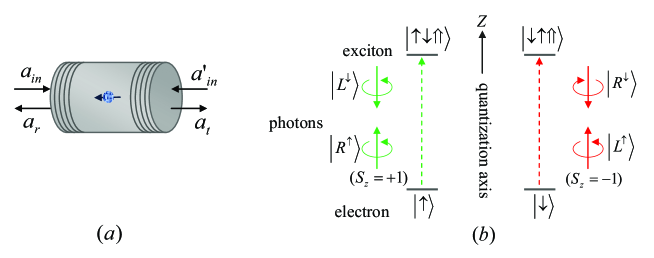
Figure 1: (a) A schematic diagram for a singly charged QD inside a double-sided optical microcavity. (b) Schematic description of the relevant exciton energy levels and the spin selection rules for optical transition of negatively charged excitons. $|R^{\uparrow}\rangle$ ($|R^{\downarrow}\rangle$) and $|L^{\uparrow}\rangle$ ($|L^{\downarrow}\rangle$) represent the right-circularly polarized photon and the left-circularly polarized photon propagating along (against) the normal direction of the cavity Z axis (the quantization axis), respectively.

II Interaction between a circularly polarized light and a single charged QD in a double-sided microcavity

A singly charged electron In(Ga)As QD or a GaAs interface QD is embedded in an optical resonant double-sided microcavity with two mirrors partially reflective in the top and the bottom, as shown in Fig. 1(a). The optical excitation of a photon and an excess electron injected into the QD can create an exciton $X^{-}$ consisting of two electrons bound to one heavy hole with negative charges, as shown in Fig. 1(b). If the excess electron in the QD is in the spin state $|\uparrow\rangle$, only the photon in the state $|R^{\uparrow}\rangle$ or $|L^{\downarrow}\rangle$ can be resonantly absorbed to create the exciton state $|\uparrow\downarrow\Uparrow\rangle$; otherwise, if the excess electron in the QD is in the spin state $|\downarrow\rangle$, only the photon in the state $|L^{\uparrow}\rangle$ or $|R^{\downarrow}\rangle$ can be resonantly absorbed to the exciton state $|\downarrow\uparrow\Downarrow\rangle$. Here $|\Uparrow\rangle$ and $|\Downarrow\rangle$ represent the heavy-hole spin state $|+\frac{3}{2}\rangle$ and $|-\frac{3}{2}\rangle$, respectively.

The dipole interaction process can be represented by Heisenberg equations for the cavity field operator $\widehat{a}$ and the exciton $X^{-}$ dipole operator $\sigma_{-}$ in the interaction picture Quant ,

$$\begin{split}\frac{d\widehat{a}}{dt}\;=\;&-\left[i(\omega_{c}-\omega)+\kappa+\frac{\kappa_{s}}{2}\right]\widehat{a}-g\sigma_{-}\\ &-\sqrt{\kappa}\,\widehat{a}_{in^{\prime}}-\sqrt{\kappa}\,\widehat{a}_{in}+\widehat{H},\\ \frac{d\sigma_{-}}{dt}\;=\;&-\left[i(\omega_{X^{-}}-\omega)+\frac{\gamma}{2}\right]\sigma_{-}-g\sigma_{z}\,\widehat{a}+\widehat{G},\\ \widehat{a}_{r}\;=\;&\widehat{a}_{in}+\sqrt{\kappa}\,\widehat{a},\;\;\;\;\;\;\;\widehat{a}_{t}\;=\;\widehat{a}_{in^{\prime}}+\sqrt{\kappa}\,\widehat{a},\end{split}$$ (1)

where $\omega$, $\omega_{c}$, and $\omega_{X^{-}}$ are the frequencies of the photon, the cavity, and $X^{-}$ transition, respectively. $g$ is the coupling constant between the $X^{-}$ and the cavity. $\kappa$ and $\kappa_{s}$ represent the cavity decay rate and the leaky rate, respectively. $\gamma$ is the exciton dipole decay rate. $\widehat{H}$ and $\widehat{G}$ are the noise operators related to reservoirs. $\widehat{a}_{in}$, $\widehat{a}_{in^{\prime}}$, $\widehat{a}_{r}$, and $\widehat{a}_{t}$ are the input and output field operators. In the weak excitation approximation, the reflection coefficient $r(\omega)$ and the transmission coefficient $t(\omega)$ of the QD-cavity system can be described by QD9 ; QD10 ; Inputoutput

$$\begin{split}r(\omega)\;=\;&1+t(\omega),\\ t(\omega)\;=\;&-\frac{\kappa[i(\omega_{X^{-}}-\omega)+\frac{\gamma}{2}]}{[i(\omega_{X^{-}}-\omega)+\frac{\gamma}{2}][i(\omega_{c}-\omega)+\kappa+\frac{\kappa_{s}}{2}]+g^{2}}.\end{split}$$ (2)

When the QD is uncoupled to the cavity (cold cavity), that is $g=0$, the reflection $r_{0}(\omega)$ and the transmission $t_{0}(\omega)$ coefficients can be written as

$$\begin{split}r_{0}(\omega)\;=\;&\frac{i(\omega_{c}-\omega)+\frac{\kappa_{s}}{2}}{i(\omega_{c}-\omega)+\kappa+\frac{\kappa_{s}}{2}},\\ t_{0}(\omega)\;=\;&-\frac{\kappa}{i(\omega_{c}-\omega)+\kappa+\frac{\kappa_{s}}{2}}.\end{split}$$ (3)

If $\omega=\omega_{c}=\omega_{X^{-}}$, the reflection and transmission coefficients of the coupled cavity and the uncoupled cavity can be simplified as

$$\begin{split}r\;=\;&1+t,\;\;\;\;\;\;\;\;\;\;\;\;t\;=\;-\frac{\frac{\gamma}{2}\kappa}{\frac{\gamma}{2}(\kappa+\frac{\kappa_{s}}{2})+g^{2}},\\ r_{0}\;=\;&\frac{\frac{\kappa_{s}}{2}}{\kappa+\frac{\kappa_{s}}{2}},\;\;\;\;\;\;\;\;t_{0}\;=\;-\frac{\kappa}{\kappa+\frac{\kappa_{s}}{2}}.\end{split}$$ (4)

The rules for optical transitions in a realistic QD-cavity system can be described as QD10 ,

$$\begin{split}&|R^{\uparrow}\uparrow\rangle\;\rightarrow\;r|L^{\downarrow}\uparrow\rangle+t|R^{\uparrow}\uparrow\rangle,\\ &|L^{\downarrow}\uparrow\rangle\;\rightarrow\;r|R^{\uparrow}\uparrow\rangle+t|L^{\downarrow}\uparrow\rangle,\\ &|R^{\downarrow}\uparrow\rangle\;\rightarrow\;t_{0}|R^{\downarrow}\uparrow\rangle+r_{0}|L^{\uparrow}\uparrow\rangle,\\ &|L^{\uparrow}\uparrow\rangle\;\rightarrow t_{0}|L^{\uparrow}\uparrow\rangle+r_{0}|R^{\downarrow}\uparrow\rangle,\\ &|R^{\downarrow}\downarrow\rangle\;\rightarrow r|L^{\uparrow}\downarrow\rangle+t|R^{\downarrow}\downarrow\rangle,\\ &|L^{\uparrow}\downarrow\rangle\;\rightarrow\;r|R^{\downarrow}\downarrow\rangle+t|L^{\uparrow}\downarrow\rangle,\\ &|R^{\uparrow}\downarrow\rangle\;\rightarrow\;t_{0}|R^{\uparrow}\downarrow\rangle+r_{0}|L^{\downarrow}\downarrow\rangle,\\ &|L^{\downarrow}\downarrow\rangle\;\rightarrow\;t_{0}|L^{\downarrow}\downarrow\rangle+r_{0}|R^{\uparrow}\downarrow\rangle.\end{split}$$ (5)

III An error-detected block for the interaction between the circularly-polarized photon and the QD-cavity system

The schematic diagram of our error-detected block for the interaction between the circularly-polarized photon and the QD-cavity system is shown in Fig. 2, which is constructed with a $50:50$ beam splitter (BS), two half-wave plates (H_pi), two mirrors (M_i), a single-photon detector (D), and a QD-cavity system. The QD in the cavity is prepared in the state $|\varphi_{+}\rangle=\frac{1}{\sqrt{2}}(|\uparrow\rangle+|\downarrow\rangle)$. If the photon is in the right-circularly polarized state $|R\rangle$, one injects it into our error-detected block from the path $i_{1}$ and lets it pass through BS and H_pi $(i=1,2)$. After being reflected by the mirror M_i $(i=1,2)$, the state of the whole system composed of the photon and the QD in the cavity is changed from the state $|\Phi\rangle_{0}=|R\rangle|i_{1}\rangle\otimes\frac{1}{\sqrt{2}}(|\uparrow\rangle+|\downarrow\rangle)$ into the state $|\Phi\rangle_{1}$. Here $|\Phi\rangle_{1}$ is

$$\begin{split}|\Phi\rangle_{1}\;=\;&\frac{1}{2}[(|R^{\downarrow}\rangle+|L^{\downarrow}\rangle)|j_{1}\rangle+(|R^{\uparrow}\rangle+|L^{\uparrow}\rangle)|j_{2}\rangle]\\ &\otimes\frac{1}{\sqrt{2}}(|\uparrow\rangle+|\downarrow\rangle).\end{split}$$ (6)

After the interaction between the photon and the QD-cavity system, the state becomes

$$\begin{split}|\Phi\rangle_{2}\;=\;&\frac{1}{2\sqrt{2}}[(t_{0}+r_{0})|R^{\downarrow}\rangle|j_{2}\rangle+(t+r)|L^{\downarrow}\rangle|j_{2}\rangle\\ &+(t+r)|R^{\uparrow}\rangle|j_{1}\rangle+(r_{0}+t_{0})|L^{\uparrow}\rangle|j_{1}\rangle]|\uparrow\rangle\\ &+\frac{1}{2\sqrt{2}}[(t_{0}+r_{0})|R^{\uparrow}\rangle|j_{1}\rangle+(t+r)|L^{\uparrow}\rangle|j_{1}\rangle\\ &+(t+r)|R^{\downarrow}\rangle|j_{2}\rangle+(t_{0}+r_{0})|L^{\downarrow}\rangle|j_{2}\rangle]|\downarrow\rangle.\end{split}$$ (7)

Subsequently, the photon is reflected by M_i $(i=1,2)$ and passes through H_pi $(i=1,2)$ again, and the state evolves to

$$\begin{split}|\Phi\rangle_{3}\;=\;&\frac{1}{4}[(t+r+t_{0}+r_{0})|R^{\downarrow}\rangle|j_{2}\rangle\\ &+(t+r+t_{0}+r_{0})|R^{\uparrow}\rangle|j_{1}\rangle\\ &-(t+r-t_{0}-r_{0})|L^{\downarrow}\rangle|j_{2}\rangle\\ &+(t+r-t_{0}-r_{0})|L^{\uparrow}\rangle|j_{1}\rangle]|\uparrow\rangle\\ &+\frac{1}{4}[(t+r+t_{0}+r_{0})|R^{\downarrow}\rangle|j_{2}\rangle\\ &+(t+r+t_{0}+r_{0})|R^{\uparrow}\rangle|j_{1}\rangle\\ &+(t+r-t_{0}-r_{0})|L^{\downarrow}\rangle|j_{2}\rangle\\ &-(t+r-t_{0}-r_{0})|L^{\uparrow}\rangle|j_{1}\rangle]|\downarrow\rangle.\end{split}$$ (8)

At last, the photon passes through BS again and the final state can be described as

$$|\Phi\rangle_{4}=D|R\rangle|i_{1}\rangle|\varphi_{+}\rangle+T|L\rangle|i_{2}\rangle|\varphi_{-}\rangle.$$ (9)

Here $D=\frac{1}{2}(t+r+t_{0}+r_{0})$ and $T=\frac{1}{2}(t+r-t_{0}-r_{0})$ are the reflection coefficient and the transmission coefficient of the error-detected block, respectively. Similarly, if the QD in the cavity is prepared in the state $|\varphi_{-}\rangle=\frac{1}{\sqrt{2}}(|\uparrow\rangle-|\downarrow\rangle)$, the outcome of the process can be described as

$$|\Phi\rangle_{5}=D|R\rangle|i_{1}\rangle|\varphi_{-}\rangle+T|L\rangle|i_{2}\rangle|\varphi_{+}\rangle.$$ (10)

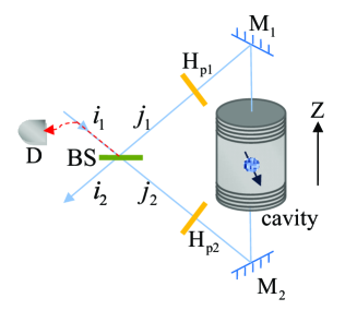
Figure 2: Schematic diagram of the error-detected block. BS is a $50:50$ beam splitter which performs the spatial-mode Hadamard operation [$|i_{1}\rangle\rightarrow\frac{1}{\sqrt{2}}(|j_{1}\rangle+|j_{2}\rangle)$, $|i_{2}\rangle\rightarrow\frac{1}{\sqrt{2}}(|j_{1}\rangle-|j_{2}\rangle)$] on the photon. H_pi $(i=1,2)$ is a half-wave plate which performs the polarization Hadamard operation [$|R\rangle\rightarrow\frac{1}{\sqrt{2}}(|R\rangle+|L\rangle)$, $|L\rangle\rightarrow\frac{1}{\sqrt{2}}(|R\rangle-|L\rangle)$] on the photon. M_i $(i=1,2)$ is a mirror. D is a single-photon detector.

One can see that there are two parts of the outcome. If the photon is reflected from the error-detected block with probability of $|D|^{2}$, the polarization of the photon and the state of the QD would not change. The reflected photon would be detected by the detector and the click of the detector represents the case in which the corresponding task of the error-detected block runs fail. If the photon is transmitted from the error-detected block with probability of $|T|^{2}$, the polarization of the photon is flipped and the superposition state of the QD is changed from $|\varphi_{+}\rangle$ to $|\varphi_{-}\rangle$ or from $|\varphi_{-}\rangle$ to $|\varphi_{+}\rangle$. We can utilize the transmitted photon and the QD-cavity to accomplish the tasks of deterministic HBSG, complete HBSA, and complete nondestructive HBSA with a high fidelity. $|D|$ and $|T|$ are affected by the $g/\kappa$ and $\kappa_{s}/\kappa$ as shown in Fig. 3. From Fig. 3, one can see that there exists a zero value of reflection coefficient, which results from the destructive interference. For the condition $g^{2}/\kappa\gamma\gg 1$ and $\kappa_{s}/2\kappa\gg 1$, the final state $|\Phi\rangle_{f1}=|L\rangle|i_{2}\rangle|\varphi_{-}\rangle$ and $|\Phi\rangle_{f2}=|L\rangle|i_{2}\rangle|\varphi_{+}\rangle$ of the error-detected block is obtained when the QD is prepared in the state $|\varphi_{+}\rangle$ and $|\varphi_{-}\rangle$, respectively.

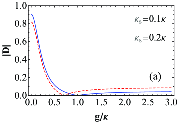
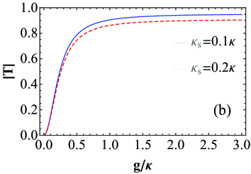
Figure 3: (a) The blue solid line and the red dashed line are the reflection coefficient $|D|$ of the error-detected block vs the normalized coupling strength $g/\kappa$ for the leakage rates $\kappa_{s}=0.1\kappa$ and $\kappa_{s}=0.2\kappa$, respectively. (b) The blue solid line and the red dashed line are the transmission coefficient $|T|$ of the error-heralded block vs $g/\kappa$ for $\kappa_{s}=0.1\kappa$ and $\kappa_{s}=0.2\kappa$, respectively. $\gamma=0.1\kappa$, which is experimentally achievable, and $\omega=\omega_{c}=\omega_{X^{-}}$ are taken here.

IV Deterministic photonic hyperentanglement generation

A two-photon four-qubit hyperentangled Bell state can be described as

$$|\Psi\rangle_{PS}=\frac{1}{2}(|RR\rangle+|LL\rangle)_{AB}(|a_{1}b_{1}\rangle+|a_{2}b_{2}\rangle)_{AB}.$$ (11)

Here the subscripts $P$ and $S$ denote the polarization and the spatial-mode DOFs, respectively. The subscripts $A$ and $B$ represent the two photons in the hyperentangled state, respectively. $|R\rangle$ and $|L\rangle$ represent the right-circular and the left-circular polarizations of photons, respectively. $|a_{1}\rangle$ ($|b_{1}\rangle$) and $|a_{2}\rangle$ ($|b_{2}\rangle$) are the different spatial modes for photon $A$ ($B$). The four Bell states in the polarization DOF can be expressed as

$$\begin{split}|\phi^{\pm}\rangle_{P}\;=\;&\frac{1}{\sqrt{2}}(|RR\rangle\pm|LL\rangle),\\ |\psi^{\pm}\rangle_{P}\;=\;&\frac{1}{\sqrt{2}}(|RL\rangle\pm|LR\rangle).\end{split}$$ (12)

The four Bell states in the spatial-mode DOF can be written as

$$\begin{split}|\phi^{\pm}\rangle_{S}\;=\;&\frac{1}{\sqrt{2}}(|a_{1}b_{1}\rangle\pm|a_{2}b_{2}\rangle),\\ |\psi^{\pm}\rangle_{S}\;=\;&\frac{1}{\sqrt{2}}(|a_{1}b_{2}\rangle\pm|a_{2}b_{1}\rangle).\end{split}$$ (13)

The principle of our scheme for the two-photon polarization-spatial hyperentangled-Bell-state generation (HBSG) constructed with two error-detected blocks and some linear optical elements is shown in Fig. 4. The QDs are prepared in the initial states $|\varphi_{+}\rangle_{1}=|\varphi_{+}\rangle_{2}$ and the two photons $A$ and $B$ with the same frequency are prepared in the same initial state $|\varphi\rangle_{A}=|\varphi\rangle_{B}=\frac{1}{\sqrt{2}}(|R\rangle+|L\rangle)$. The process for HBSG can be described in detail as follows.

Figure 4: Schematic diagram for two-photon polarization-spatial HBSG. CPBS_i $(i=1,2,3)$ is a circularly polarized beam splitter which transmits the photon in the left-circular polarization $|L\rangle$ and reflects the photon in the right-circular polarization $|R\rangle$, respectively. X_i $(i=1,2,3)$ is a half-wave plate which performs a polarization bit-flip operation $\sigma_{x}^{p}=|R\rangle\langle L|+|L\rangle\langle R|$ on the photon.

First, one injects photon $A$ into the quantum circuit from the left input, followed by photon $B$. The time interval $\Delta t$ exists between photons $A$ and $B$, and $\Delta t$ should be less than the spin coherence time $\Gamma$. CPBS₁ will transmit the photon to path $a_{1}$ $(b_{1})$ and reflects the photon to path $a_{2}$ $(b_{2})$ when photon $A$ $(B)$ is in the state $|L\rangle$ and $|R\rangle$, respectively. When photon $A$ $(B)$ emerges in path $a_{2}$ $(b_{2})$, it passes through the error-detected block consisting of the QD-cavity₁ system and X₁. Before the two wave packets split by CPBS₁ interfere at BS₂, the state of the whole system is changed from $\Omega_{0}=|\varphi\rangle_{A}|\varphi\rangle_{B}|\varphi_{+}\rangle_{1}|\varphi_{+}\rangle_{2}$ to $\Omega_{1}$. Here $\Omega_{1}$ is written as

$$\begin{split}\Omega_{1}=&\frac{1}{2}(|LL\rangle|a_{1}b_{1}\rangle|\varphi_{+}\rangle_{1}+|LR\rangle|a_{1}b_{2}\rangle|\varphi_{-}\rangle_{1}\\ &+|RL\rangle|a_{2}b_{1}\rangle|\varphi_{-}\rangle_{1}+|RR\rangle|a_{2}b_{2}\rangle|\varphi_{+}\rangle_{1})|\varphi_{+}\rangle_{2}.\end{split}$$ (14)

Then BS₂, which performs the spatial-mode Hadamard operation [$|a_{1}(b_{1})\rangle\rightarrow\frac{1}{\sqrt{2}}(|c_{1}(|d_{1})\rangle+|c_{2}(d_{2})\rangle$, $|a_{2}(b_{2})\rangle\rightarrow\frac{1}{\sqrt{2}}(|c_{1}(|d_{1})\rangle-|c_{2}(d_{2})\rangle$] on photons transmitted, will lead photon $A$ $(B)$ to paths $c_{1}$ $(d_{1})$ and $c_{2}$ $(d_{2})$. In path $c_{2}$ $(d_{2})$, photon $A$ $(B)$ passes through CPBS₂ which transmits the photon $A$ $(B)$ in $|L\rangle$ and reflects the photon in $|R\rangle$, respectively. Then photon $A$ $(B)$ in $|L\rangle$ takes a $\sigma_{x}^{p}$ operation by X₂ and passes through the error-detected block consisting of QD-cavity₂ system, sequently. Photon $A$ $(B)$ in $|R\rangle$ passes through the same error-detected block and takes a $\sigma_{x}^{p}$ operation by X₃, sequentially. At last, the two wave packets union at CPBS₃ in path $a_{2}$ $(b_{2})$. The state of the whole system becomes

$$\begin{split}\Omega_{2}\;=\;&\frac{1}{2}(|\phi^{+}\rangle_{P}|\phi^{+}\rangle_{S}|\varphi_{+}\rangle_{1}|\varphi_{+}\rangle_{2}\\ &-|\phi^{-}\rangle_{P}|\psi^{+}\rangle_{S}|\varphi_{+}\rangle_{1}|\varphi_{-}\rangle_{2}\\ &+|\psi^{+}\rangle_{P}|\phi^{-}\rangle_{S}|\varphi_{-}\rangle_{1}|\varphi_{+}\rangle_{2}\\ &+|\psi^{-}\rangle_{P}|\psi^{-}\rangle_{S}|\varphi_{-}\rangle_{1}|\varphi_{-}\rangle_{2}).\end{split}$$ (15)

From Eq. (15), one can see the relationship between the measurement outcomes of the two QD-cavity systems and the polarization-spatial hyperentangled Bell states of the two-photon system. If QD₁ and QD₂ are in the states $|\varphi_{+}\rangle_{1}$ and $|\varphi_{+}\rangle_{2}$, respectively, the two-photon system is in the hyperentangled Bell state $|\phi^{+}\rangle_{P}|\phi^{+}\rangle_{S}$. If QD₁ and QD₂ are in the states $|\varphi_{+}\rangle_{1}$ and $|\varphi_{-}\rangle_{2}$, respectively, the two-photon system is in the hyperentangled Bell state $|\phi^{-}\rangle_{P}|\psi^{+}\rangle_{S}$. When QD₁ and QD₂ are in the states $|\varphi_{-}\rangle_{1}$ and $|\varphi_{+}\rangle_{2}$, respectively, the two-photon system is in the hyperentangled Bell state $|\psi^{+}\rangle_{P}|\phi^{-}\rangle_{S}$. When QD₁ and QD₂ are in the states $|\varphi_{-}\rangle_{1}$ and $|\varphi_{-}\rangle_{2}$, respectively, the two-photon system is in the hyperentangled Bell state $|\psi^{-}\rangle_{P}|\psi^{-}\rangle_{S}$. Therefore, one can generate deterministically a polarization-spatial hyperentangled Bell state of the two-photon system by measuring the states of the two QDs. Other polarization-spatial hyperentangled Bell states can be generated with some appropriate single-qubit operations.

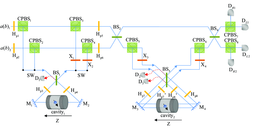
Figure 5: Schematic diagram of the complete polarization-spatial HBSA. D_i $(i=1,2,3)$, D_Li $(i=1,2)$ and D_Ri $(i=1,2)$ are single-photon detectors. SW is an optical switch which lets the wave-packets of a photon in different spatial-mode pass into and out of the error-detected block sequentially.

V Complete polarization-spatial hyperentangled Bell states analysis

The schematic diagram of the complete polarization-spatial HBSA for hyperentangled two-photon systems is shown in Fig. 5. Here we use two error-detected blocks consisting of two QD-cavity systems and some linear optical elements to achieve the complete polarization-spatial HBSA. The two QDs are prepared in the initial states $|\varphi_{+}\rangle_{1}=|\varphi_{+}\rangle_{2}$ and the hyperentangled two-photon system is in one of the $16$ hyperentangled Bell states. The process for our HBSA can be described as follows.

One lets photon $A$ pass through the quantum circuit from the left input port, followed by photon $B$. And the two photons will be detected sequentially at the output port. The interval time $\Delta t$ existing between the two photons is less than the spin coherence time $\Gamma$. According to the results of the interaction between the circularly polarized photon and the error-detected block, after the two photons $A$ and $B$ pass through quantum circuit and before they are detected by the detectors (D_Ri and D_Li), the whole system composed of the two photons and the two QDs evolves as

$$\begin{split}&|\phi^{+}\rangle_{P}(|\psi^{+}\rangle_{P})|\phi^{+}\rangle_{S}|\varphi_{+}\rangle_{1}|\varphi_{+}\rangle_{2}\;\;\,\rightarrow\;\;|\phi^{+}\rangle_{P}(|\psi^{+}\rangle_{P})|\phi^{+}\rangle_{S}|\varphi_{+}\rangle_{1}|\varphi_{+}\rangle_{2},\\ &|\phi^{+}\rangle_{P}(|\psi^{+}\rangle_{P})|\psi^{+}\rangle_{S}|\varphi_{+}\rangle_{1}|\varphi_{+}\rangle_{2}\;\;\rightarrow\;\;|\phi^{+}\rangle_{P}(|\psi^{+}\rangle_{P})|\psi^{+}\rangle_{S}|\varphi_{+}\rangle_{1}|\varphi_{+}\rangle_{2},\\ &|\phi^{+}\rangle_{P}(|\psi^{+}\rangle_{P})|\phi^{-}\rangle_{S}|\varphi_{+}\rangle_{1}|\varphi_{+}\rangle_{2}\;\;\,\rightarrow\;\;|\phi^{+}\rangle_{P}(|\psi^{+}\rangle_{P})|\phi^{-}\rangle_{S}|\varphi_{+}\rangle_{1}|\varphi_{-}\rangle_{2},\\ &|\phi^{+}\rangle_{P}(|\psi^{+}\rangle_{P})|\psi^{-}\rangle_{S}|\varphi_{+}\rangle_{1}|\varphi_{+}\rangle_{2}\;\;\rightarrow\;\;|\phi^{+}\rangle_{P}(|\psi^{+}\rangle_{P})|\psi^{-}\rangle_{S}|\varphi_{+}\rangle_{1}|\varphi_{-}\rangle_{2},\\ &|\phi^{-}\rangle_{P}(|\psi^{-}\rangle_{P})|\phi^{+}\rangle_{S}|\varphi_{+}\rangle_{1}|\varphi_{+}\rangle_{2}\;\;\,\rightarrow\;\;|\phi^{-}\rangle_{P}(|\psi^{-}\rangle_{P})|\phi^{+}\rangle_{S}|\varphi_{-}\rangle_{1}|\varphi_{+}\rangle_{2},\\ &|\phi^{-}\rangle_{P}(|\psi^{-}\rangle_{P})|\psi^{+}\rangle_{S}|\varphi_{+}\rangle_{1}|\varphi_{+}\rangle_{2}\;\;\rightarrow\;\;|\phi^{-}\rangle_{P}(|\psi^{-}\rangle_{P})|\psi^{+}\rangle_{S}|\varphi_{-}\rangle_{1}|\varphi_{+}\rangle_{2},\\ &|\phi^{-}\rangle_{P}(|\psi^{-}\rangle_{P})|\phi^{-}\rangle_{S}|\varphi_{+}\rangle_{1}|\varphi_{+}\rangle_{2}\;\;\,\rightarrow\;\;|\phi^{-}\rangle_{P}(|\psi^{-}\rangle_{P})|\phi^{-}\rangle_{S}|\varphi_{-}\rangle_{1}|\varphi_{-}\rangle_{2},\\ &|\phi^{-}\rangle_{P}(|\psi^{-}\rangle_{P})|\psi^{-}\rangle_{S}|\varphi_{+}\rangle_{1}|\varphi_{+}\rangle_{2}\;\;\rightarrow\;\;|\phi^{-}\rangle_{P}(|\psi^{-}\rangle_{P})|\psi^{-}\rangle_{S}|\varphi_{-}\rangle_{1}|\varphi_{-}\rangle_{2}.\end{split}$$ (16)

At last, the photons $A$ and $B$ are independently measured in both the polarization and the spatial-mode DOFs with single-photon detectors, and the two QDs are measured in the basis $\{|\varphi_{+}\rangle,|\varphi_{-}\rangle\}$. The relationship between the measurement outcomes and the initial hyperentangled states of the two-photon system $AB$ is shown in Table 1.

Table 1: The relationship between the measurement outcomes of the states of the two-photon systems in the polarization and spatial-mode DOFs and the two QDs and the initial hyperentangled states of the two-photon system $|\Psi\rangle_{PS}$.

QD1 and QD2	Polarization	Spatial-mode	$|\Psi\rangle_{PS}$
$|\varphi_{+}\rangle_{1}|\varphi_{+}\rangle_{2}$	$RR$, $LL$	$a_{1}b_{1}$, $a_{2}b_{2}$	$|\phi^{+}\rangle_{P}|\phi^{+}\rangle_{S}$
$|\varphi_{+}\rangle_{1}|\varphi_{+}\rangle_{2}$	$RR$, $LL$	$a_{1}b_{2}$, $a_{2}b_{1}$	$|\phi^{+}\rangle_{P}|\psi^{+}\rangle_{S}$
$|\varphi_{+}\rangle_{1}|\varphi_{+}\rangle_{2}$	$RL$, $LR$	$a_{1}b_{1}$, $a_{2}b_{2}$	$|\psi^{+}\rangle_{P}|\phi^{+}\rangle_{S}$
$|\varphi_{+}\rangle_{1}|\varphi_{+}\rangle_{2}$	$RL$, $LR$	$a_{1}b_{2}$, $a_{2}b_{1}$	$|\psi^{+}\rangle_{P}|\psi^{+}\rangle_{S}$
$|\varphi_{+}\rangle_{1}|\varphi_{-}\rangle_{2}$	$RR$, $LL$	$a_{1}b_{1}$, $a_{2}b_{2}$	$|\phi^{+}\rangle_{P}|\phi^{-}\rangle_{S}$
$|\varphi_{+}\rangle_{1}|\varphi_{-}\rangle_{2}$	$RR$, $LL$	$a_{1}b_{2}$, $a_{2}b_{1}$	$|\phi^{+}\rangle_{P}|\psi^{-}\rangle_{S}$
$|\varphi_{+}\rangle_{1}|\varphi_{-}\rangle_{2}$	$RL$, $LR$	$a_{1}b_{1}$, $a_{2}b_{2}$	$|\psi^{+}\rangle_{P}|\phi^{-}\rangle_{S}$
$|\varphi_{+}\rangle_{1}|\varphi_{-}\rangle_{2}$	$RL$, $LR$	$a_{1}b_{2}$, $a_{2}b_{1}$	$|\psi^{+}\rangle_{P}|\psi^{-}\rangle_{S}$
$|\varphi_{-}\rangle_{1}|\varphi_{+}\rangle_{2}$	$RR$, $LL$	$a_{1}b_{1}$, $a_{2}b_{2}$	$|\phi^{-}\rangle_{P}|\phi^{+}\rangle_{S}$
$|\varphi_{-}\rangle_{1}|\varphi_{+}\rangle_{2}$	$RR$, $LL$	$a_{1}b_{2}$, $a_{2}b_{1}$	$|\phi^{-}\rangle_{P}|\psi^{+}\rangle_{S}$
$|\varphi_{-}\rangle_{1}|\varphi_{+}\rangle_{2}$	$RL$, $LR$	$a_{1}b_{1}$, $a_{2}b_{2}$	$|\psi^{-}\rangle_{P}|\phi^{+}\rangle_{S}$
$|\varphi_{-}\rangle_{1}|\varphi_{+}\rangle_{2}$	$RL$, $LR$	$a_{1}b_{2}$, $a_{2}b_{1}$	$|\psi^{-}\rangle_{P}|\psi^{+}\rangle_{S}$
$|\varphi_{-}\rangle_{1}|\varphi_{-}\rangle_{2}$	$RR$, $LL$	$a_{1}b_{1}$, $a_{2}b_{2}$	$|\phi^{-}\rangle_{P}|\phi^{-}\rangle_{S}$
$|\varphi_{-}\rangle_{1}|\varphi_{-}\rangle_{2}$	$RR$, $LL$	$a_{1}b_{2}$, $a_{2}b_{1}$	$|\phi^{-}\rangle_{P}|\psi^{-}\rangle_{S}$
$|\varphi_{-}\rangle_{1}|\varphi_{-}\rangle_{2}$	$RL$, $LR$	$a_{1}b_{1}$, $a_{2}b_{2}$	$|\psi^{-}\rangle_{P}|\phi^{-}\rangle_{S}$
$|\varphi_{-}\rangle_{1}|\varphi_{-}\rangle_{2}$	$RL$, $LR$	$a_{1}b_{2}$, $a_{2}b_{1}$	$|\psi^{-}\rangle_{P}|\psi^{-}\rangle_{S}$

From Table 1, one can obtain the complete and deterministic analysis on hyperentangled Bell states of a two-photon system $AB$. The measurement outcomes of QD₁ and QD₂ reveal the phase information in the polarization and the spatial-mode DOFs, respectively. In detail, when QD₁ (QD${}_{2})$ is in the spin state $|\varphi_{+}\rangle_{1}$ $(|\varphi_{+}\rangle_{2})$, the two-photon system is in the states $|\phi^{+}\rangle_{P(S)}$ or $|\psi^{+}\rangle_{P(S)}$ in the polarization (spatial-mode) DOF. Otherwise, when QD₁ (QD${}_{2})$ is in the spin state $|\varphi_{-}\rangle_{1}$ $(|\varphi_{-}\rangle_{2})$, the two-photon system is in the states $|\phi^{-}\rangle_{P(S)}$ or $|\psi^{-}\rangle_{P(S)}$ in the polarization (spatial-mode) DOF. The measurement outcomes of the states of the two-photon system in the polarization DOF reveal the parity information in the polarization DOF. In detail, if the measurement outcome of the state is $RR$ or $LL$, the two-photon system is in the state $|\phi^{\pm}\rangle_{P}$ in the polarization DOF; otherwise, it is in the state $|\psi^{\pm}\rangle_{P}$. The measurement outcomes of the states of the two-photon system in the spatial-mode DOF reveal the parity information in the spatial-mode DOF. In detail, if the measurement outcome of the state is $a_{1}b_{1}$ or $a_{2}b_{2}$, the two-photon system is in the state $|\phi^{\pm}\rangle_{S}$; otherwise, it is in the state $|\psi^{\pm}\rangle_{S}$. That is, the schematic diagram shown in Fig. 5 can be used for the complete and deterministic HBSA.

Table 2: The relationship between the measurement outcomes of the states of the four QDs and the initial hyperentangled states of the two-photon system $|\Psi\rangle_{PS}$.

QD1	QD2	QD3	QD4	$|\Psi\rangle_{PS}$
$|\varphi_{+}\rangle_{1}$	$|\varphi_{+}\rangle_{2}$	$|\varphi_{+}\rangle_{3}$	$|\varphi_{+}\rangle_{4}$	$|\phi^{+}\rangle_{P}|\phi^{+}\rangle_{S}$
$|\varphi_{-}\rangle_{1}$	$|\varphi_{+}\rangle_{2}$	$|\varphi_{+}\rangle_{3}$	$|\varphi_{+}\rangle_{4}$	$|\psi^{+}\rangle_{P}|\phi^{+}\rangle_{S}$
$|\varphi_{+}\rangle_{1}$	$|\varphi_{-}\rangle_{2}$	$|\varphi_{+}\rangle_{3}$	$|\varphi_{+}\rangle_{4}$	$|\phi^{-}\rangle_{P}|\phi^{+}\rangle_{S}$
$|\varphi_{-}\rangle_{1}$	$|\varphi_{-}\rangle_{2}$	$|\varphi_{+}\rangle_{3}$	$|\varphi_{+}\rangle_{4}$	$|\psi^{-}\rangle_{P}|\phi^{+}\rangle_{S}$
$|\varphi_{+}\rangle_{1}$	$|\varphi_{+}\rangle_{2}$	$|\varphi_{-}\rangle_{3}$	$|\varphi_{+}\rangle_{4}$	$|\phi^{+}\rangle_{P}|\psi^{+}\rangle_{S}$
$|\varphi_{-}\rangle_{1}$	$|\varphi_{+}\rangle_{2}$	$|\varphi_{-}\rangle_{3}$	$|\varphi_{+}\rangle_{4}$	$|\psi^{+}\rangle_{P}|\psi^{+}\rangle_{S}$
$|\varphi_{+}\rangle_{1}$	$|\varphi_{-}\rangle_{2}$	$|\varphi_{-}\rangle_{3}$	$|\varphi_{+}\rangle_{4}$	$|\phi^{-}\rangle_{P}|\psi^{+}\rangle_{S}$
$|\varphi_{-}\rangle_{1}$	$|\varphi_{-}\rangle_{2}$	$|\varphi_{-}\rangle_{3}$	$|\varphi_{+}\rangle_{4}$	$|\psi^{-}\rangle_{P}|\psi^{+}\rangle_{S}$
$|\varphi_{+}\rangle_{1}$	$|\varphi_{+}\rangle_{2}$	$|\varphi_{+}\rangle_{3}$	$|\varphi_{-}\rangle_{4}$	$|\phi^{+}\rangle_{P}|\phi^{-}\rangle_{S}$
$|\varphi_{-}\rangle_{1}$	$|\varphi_{+}\rangle_{2}$	$|\varphi_{+}\rangle_{3}$	$|\varphi_{-}\rangle_{4}$	$|\psi^{+}\rangle_{P}|\phi^{-}\rangle_{S}$
$|\varphi_{+}\rangle_{1}$	$|\varphi_{-}\rangle_{2}$	$|\varphi_{+}\rangle_{3}$	$|\varphi_{-}\rangle_{4}$	$|\phi^{-}\rangle_{P}|\phi^{-}\rangle_{S}$
$|\varphi_{-}\rangle_{1}$	$|\varphi_{-}\rangle_{2}$	$|\varphi_{+}\rangle_{3}$	$|\varphi_{-}\rangle_{4}$	$|\psi^{-}\rangle_{P}|\phi^{-}\rangle_{S}$
$|\varphi_{+}\rangle_{1}$	$|\varphi_{+}\rangle_{2}$	$|\varphi_{-}\rangle_{3}$	$|\varphi_{-}\rangle_{4}$	$|\phi^{+}\rangle_{P}|\psi^{-}\rangle_{S}$
$|\varphi_{-}\rangle_{1}$	$|\varphi_{+}\rangle_{2}$	$|\varphi_{-}\rangle_{3}$	$|\varphi_{-}\rangle_{4}$	$|\psi^{+}\rangle_{P}|\psi^{-}\rangle_{S}$
$|\varphi_{+}\rangle_{1}$	$|\varphi_{-}\rangle_{2}$	$|\varphi_{-}\rangle_{3}$	$|\varphi_{-}\rangle_{4}$	$|\phi^{-}\rangle_{P}|\psi^{-}\rangle_{S}$
$|\varphi_{-}\rangle_{1}$	$|\varphi_{-}\rangle_{2}$	$|\varphi_{-}\rangle_{3}$	$|\varphi_{-}\rangle_{4}$	$|\psi^{-}\rangle_{P}|\psi^{-}\rangle_{S}$

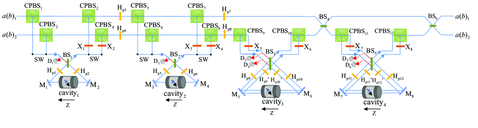
Figure 6: Schematic diagram of the complete nondestructive polarization-spatial HBSA.

VI Complete nondestructive polarization-spatial hyperentangled Bell-state analysis

The protocol for the complete polarization-spatial HBSA proposed in the former section is destructive. After the analysis of two-photon polarization-spatial hyperentangled Bell states, the two photons are detected at last and they cannot be used for other quantum information processing tasks. In this section, we propose a complete nondestructive polarization-spatial HBSA. The schematic diagram of the complete nondestructive polarization-spatial HBSA is shown in Fig. 6. The four QDs are all prepared in the states $|\varphi_{+}\rangle_{1}=|\varphi_{+}\rangle_{2}=|\varphi_{+}\rangle_{3}=|\varphi_{+}\rangle_{4}$ and the hyperentangled two-photon system is in one of the $16$ hyperentangled Bell states.

One lets photon $A$ pass through the quantum circuit from the left input port, followed by photon $B$. The interval time $\Delta t$, which is less than the spin coherence time $\Gamma$, exists between the two photons. After the two photons $A$ and $B$ passes through quantum circuit, the evolution of the system composed of two photons and four QDs is shown in Table 2.

From Table 2, one can obtain the complete and deterministic analysis on hyperentangled Bell states of a two-photon system $AB$ without detecting it. The measurement outcomes of QD₁ and QD₃ show the parity information in the polarization DOF and the spatial-mode DOF, respectively. In detail, when QD₁ (QD${}_{3})$ is in the state $|\varphi_{+}\rangle_{1}$ ($|\varphi_{+}\rangle_{3}$), the two-photon system is in the state $|\phi^{\pm}\rangle_{P(S)}$ in the polarization (spatial-mode) DOF. Otherwise, when QD₁ ($QD_{3})$ is in the state $|\varphi_{-}\rangle_{1}$ ($|\varphi_{-}\rangle_{3}$), the two-photon system is in the state $|\psi^{\pm}\rangle_{P(S)}$ in the polarization (spatial-mode) DOF. The measurement outcomes of QD₂ and QD₄ show the phase information in the polarization DOF and the spatial-mode DOF, respectively. In detail, when QD₂ (QD₄) is in the state $|\varphi_{+}\rangle_{2}$ ($|\varphi_{+}\rangle_{4}$), the two-photon system is in the state $|\phi^{+}\rangle_{P(S)}$ or $|\psi^{+}\rangle_{P(S)}$ in the polarization (spatial-mode) DOF. Otherwise, when QD₂ (QD₄) is in the state $|\varphi_{-}\rangle_{2}$ ($|\varphi_{-}\rangle_{4}$), the two-photon system is in the state $|\phi^{-}\rangle_{P(S)}$ or $|\psi^{-}\rangle_{P(S)}$ in the polarization (spatial-mode) DOF. That is, the schematic diagram shown in Fig. 6 can be used for the complete nondestructive polarization-spatial HBSA in a deterministic way.

VII Discussion and summary

Assisted by the optical transitions in a QD-cavity system, we construct an error-detected block. With the error-detected block, our schemes for the deterministic HBSG, complete HBSA, and complete nondestructive HBSA of the polarization-spatial hyperentangled two-photon system are proposed. In an ideal condition, $|\Phi\rangle_{f1}=|L\rangle|i_{2}\rangle|\varphi_{-}\rangle$ or $|\Phi\rangle_{f2}=|L\rangle|i_{2}\rangle|\varphi_{+}\rangle$ can be obtained after the right-polarized photon $|R\rangle$ interacting with the error-detected block and the fidelities and the efficiencies of our schemes can be $100\%$. However, in a realistic condition, the outcomes of the interaction between the right-polarized photon $|R\rangle$ and the error-detected block, which are described as Eqs. (9) and (10), are affected by the coupling constant between $X^{-}$ and the cavity $g$, the cavity decay rate $\kappa$, the leaky rate $\kappa_{s}$, and the exciton dipole decay rate $\gamma$, which would affect the fidelities and the efficiencies as well.

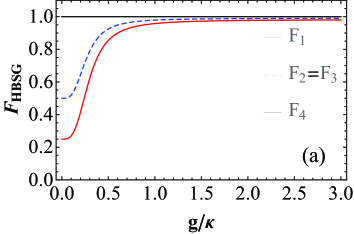
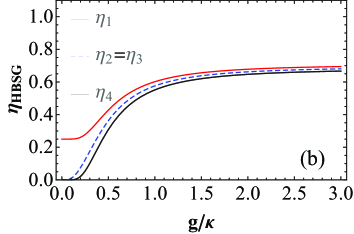
Figure 7: The performance of our deterministic HBSG scheme. The bule dashed line, the red solid line, and the black solid line describe the performance of our deterministic HBSG scheme for generating hyperentangled Bell states $|\phi^{+}\rangle_{P}|\phi^{+}\rangle_{S}$, $|\phi^{-}\rangle_{P}|\psi^{+}\rangle_{S}$, $|\psi^{+}\rangle_{P}|\phi^{-}\rangle_{S}$, and $|\psi^{-}\rangle_{P}|\psi^{-}\rangle_{S}$, respectively. (a) The fidelities of our deterministic HBSG scheme. (b) The efficiencies of our deterministic HBSG. $\gamma=0.1\kappa$ and $\kappa_{s}=0.2\kappa$, which are experimentally achievable, are taken here.

The fidelity of the process for deterministic HBSG, complete HBSA, or complete nondestructive HBSA is defined as $F=|\langle\psi_{r}|\psi_{i}\rangle|^{2}$. Here $|\psi_{r}\rangle$ and $|\psi_{i}\rangle$ are the final states in the realistic condition and ideal condition, respectively. The efficiency is defined as the ratio of the number of the output photons to the input photons. The fidelities of our scheme for deterministic HBSG are described as

$$\begin{split}F_{1}\;=\;&\frac{(T^{2}+1)^{4}}{4(T^{4}+1)^{2}},\\ F_{2}\;=\;&F_{3}\;=\;\frac{(1+T^{2})^{2}}{2(1+T^{4})},\\ F_{4}\;=\;&1.\end{split}$$ (17)

Here $F_{1}$, $F_{2}$, $F_{3}$ and $F_{4}$ are the fidelities of generating the hyperentangled Bell states $|\phi^{+}\rangle_{P}|\phi^{+}\rangle_{S}$, $|\phi^{-}\rangle_{P}|\psi^{+}\rangle_{S}$, $|\psi^{+}\rangle_{P}|\phi^{-}\rangle_{S}$, and $|\psi^{-}\rangle_{P}|\psi^{-}\rangle_{S}$, respectively. The fidelity of generating the hyperentangled Bell state $|\psi^{-}\rangle_{P}|\psi^{-}\rangle_{S}$ is unity. The efficiencies of generating these four hyperentangled states with our scheme of deterministic HBSG are described as

$$\begin{split}\eta_{1}\;=\;&\frac{1}{4}(T^{4}+1),\\ \eta_{2}\;=\;&\eta_{3}\;=\;\frac{1}{2}(T^{2}+T^{6}),\\ \eta_{4}\;=\;&T^{4}.\end{split}$$ (18)

The fidelities and the efficiencies of our deterministic HBSG scheme vary with the parameter $g/\kappa$ in the conditions of $\gamma=0.1\kappa$ and $\kappa_{s}=0.2\kappa$ are shown in Figs. 7(a) and (b), respectively. From Figs. 7(a) and (b), one can see that when $g/\kappa=0.5$, which is a low-Q-factor of a cavity, the fidelities are $F_{1}=85.45\%$ and $F_{2}=F_{3}=92.44\%$ and the efficiencies are $\eta_{1}=42.79\%$, $\eta_{2}=\eta_{3}=36.32\%$, and $\eta_{4}=30.83\%$ in the conditions $\gamma=0.1\kappa$ and $\kappa_{s}=0.2\kappa$. For a strong coupling between the QDs and the cavity, $g/\kappa>1$, the fidelities are $F_{1}>95.78\%$ and $F_{2}=F_{3}>97.86\%$, and the efficiencies are $\eta_{1}>60.17\%$, $\eta_{2}=\eta_{3}>57.60\%$, and $\eta_{4}>55.13\%$ in the conditions $\gamma=0.1\kappa$ and $\kappa_{s}=0.2\kappa$.

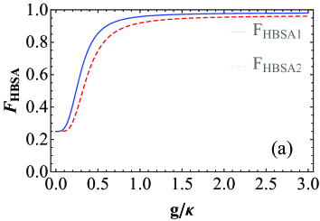
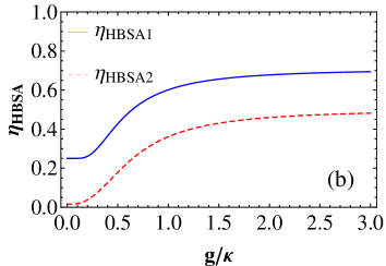
Figure 8: The performance of our complete HBSA scheme and complete nondestructive HBSA scheme for the hyperentangled Bell state $|\phi^{+}\rangle_{P}|\phi^{+}\rangle_{S}$. The blue solid line and the red dashed line describe the performance of our complete HBSA and complete nondestructive HBSA schemes, respectively. (a) The fidelities of our complete HBSA scheme and complete nondestructive HBSA scheme. (b) The efficiencies of our complete HBSA scheme and complete nondestructive HBSA scheme. $\gamma=0.1\kappa$ and $\kappa_{s}=0.2\kappa$, which are experimentally achievable, are taken here.

The fidelity and the efficiency of our complete HBSA scheme for the hyperentangled Bell state $|\phi^{+}\rangle_{P}|\phi^{+}\rangle_{S}$ are described as

$$\begin{split}&F_{HBSA1}=\frac{(T^{2}+1)^{4}}{(T^{2}+1)^{4}+2(1-T^{4})^{2}+(1-T^{2})^{4}},\\ &\eta_{HBSA1}=\frac{1}{16}[(T^{2}+1)^{4}+2(1-T^{4})^{2}+(1-T^{2})^{4}].\end{split}$$ (19)

They vary with the parameter $g/\kappa$, shown as the blue solid lines in Figs. 8(a) and (b), respectively. The fidelity and the efficiency of our complete nondestructive HBSA scheme for the hyperentangled Bell state $|\phi^{+}\rangle_{P}|\phi^{+}\rangle_{S}$ are given by

$$\begin{split}&F_{HBSA2}=\frac{(1\!+\!T^{2})^{8}}{[(1\!+\!T^{2})^{4}\!+\!(1\!-\!T^{4})^{2}\!+\!4T^{2}(1\!-\!T^{2})^{2}]^{2}},\\ &\eta_{HBSA2}=\frac{1}{256}[(1\!+\!T^{2})^{4}\!+\!(1\!-\!T^{4})^{2}\!+\!4T^{2}(1\!-\!T^{2})^{2}]^{2}.\;\;\;\;\end{split}$$ (20)

The red dashed lines in Figs. 8(a) and (b) describe $F_{HBSG2}$ and $\eta_{HBSG2}$ varying with the parameter $g/\kappa$, respectively. When the parameter $g/\kappa$ is larger than $1$, the fidelities of our complete HBSA scheme and complete nondestructive HBSA scheme will be higher than $F_{HBSA1}=95.78\%$ and $F_{HBSA2}=91.89\%$, respectively, for the hyperentangled Bell state $|\phi^{+}\rangle_{P}|\phi^{+}\rangle_{S}$ in the conditions $\gamma=0.1\kappa$ and $\kappa_{s}=0.2\kappa$. And the efficiencies will be higher than $\eta_{HBSA1}=60.17\%$ and $\eta_{HBSA2}=36.13\%$.

Besides the parameters $g$, $\kappa$, $\kappa_{s}$ and $\gamma$, the fidelities would also be affected by the exciton dephasing, including the optical dephasing and the spin dephasing of $X^{-}$. Exciton dephasing reduces the fidelity by the amount of $[1-exp(-\tau/\Gamma)]$, where $\tau$ and $\Gamma$ are the cavity photon lifetime and the trion coherence time, respectively. The optical dephasing reduces the fidelity less than $10\%$, because the time scale of the excitons can reach hundreds of picoseconds t1 ; t2 ; t3 , while the cavity photon lifetime is in the tens of picoseconds range for a self-assembled In(Ga)As-based QD with a cavity $Q$ factor of $10^{4}-10^{5}$ in the strong coupling regime. The effect of the spin dephasing can be neglected because the spin decoherence time is several orders of magnitude longer than the cavity photon lifetime t4 ; t5 ; t6 .

In addition, the fidelity can be affected by the imperfect optical selection induced by heavy-light hole mixing c62 . However, this imperfect mixing can be reduced by engineering the shape and the size of QDs or by choosing the types of QDs.

As the three protocols for deterministic HBSG, complete HBSA, and complete nondestructive HBSA are constructed by our error-detected block, the errors are detectable and the fidelities are improved. The low efficiencies can be remedied by repeat until success. Once our protocols succeeds, which means the detectors of the error-detected block don’t click, the high fidelities can be obtained. This feature seems more important in the protocol for deterministic HBSG, which means high-quality hyperentangled Bell states can be generated.

In our schemes, the spin superposition state $|\varphi_{+}\rangle$ is prepared initially. It can be prepared from the spin eigenstates by using nanosecond electron-spin-resonance pulses or picosecond optical pulses. The preparation time for the spin superposition state can be significantly shorter than $\Gamma$ because of the ultrafast optical coherent control of electron spins in semiconductor quantum wells and in semiconductor QDs. The measurement of the spin superposition state in the basis $\{|\varphi_{+}\rangle,|\varphi_{-}\rangle\}$ is required in each scheme. By applying a Hadamard operation on the electron spin, the spin superposition states $|\varphi_{+}\rangle$ and $|\varphi_{-}\rangle$ can be transformed into the spin states $|\uparrow\rangle$ and $|\downarrow\rangle$, which can be detected by measuring the helicity of the transmitted or reflected photon.

In our proposal, the two cavity modes with right- and left- circular polarizations, which couple to the two transitions $|\uparrow\rangle\leftrightarrow|\uparrow\downarrow\Uparrow\rangle$ and $|\downarrow\rangle\leftrightarrow|\downarrow\uparrow\Downarrow\rangle$, respectively, are required. Many good experiments that provide a cavity supporting both of two circularly-polarized modes with the same frequency have been realized modes1 ; modes4 ; modes6 ; modes7 . For example, Luxmoore et al. modes1 presented a technique for fine tuning of the energy split between the two circularly-polarized modes to just 0.15 nm in 2012.

In summary, we have proposed some schemes for the deterministic HBSG, the complete HBSA, and the complete nondestructive HBSA of the polarization-spatial hyperentangled two-photon system assisted by our error-detected block. The error-detected block is constructed by the optical transitions in QD-cavity system. With the help of our error-detected block, the errors can be detected, which is far different from other previous schemes assisted by the interaction between the photon and the QD-cavity system. Maybe this good feature makes our schemes more useful in long-distance quantum communication in the future.

Funding

National Natural Science Foundation of China (11674033, 11474026, 11505007, 11547106); Fundamental Research Funds for the Central Universities (2015KJJCA01); Youth Scholars Program of Beijing Normal University (2014NT28); Open Research Fund Program of the State Key Laboratory of Low Dimensional Quantum Physics, Tsinghua University (KF201502).

References

- (1) M. A. Nielsen and I. L. Chuang, Quantum Computation and Quantum Information (Cambridge University, 2000).
- (2) C. H. Bennett, G. Brassard, C. Crepeau, R. Jozsa, A. Peres, and W. K. Wootters, “Teleporting an unknown quantum state via dual classical and Einstein-Podolsky-Rosen channels,” Phys. Rev. Lett. 70, 1895 (1993).
- (3) C. H. Bennett and S. J. Wiesner, “Communication via one- and two-particle operators on Einstein-Podolsky-Rosen states,” Phys. Rev. Lett. 69, 2881–2884 (1992).
- (4) X. S. Liu, G. L. Long, D. M. Tong, and F. Li, “General scheme for superdense coding between multiparties,” Phys. Rev. A 65, 022304 (2002).
- (5) A. K. Ekert, “Quantum cryptography based on Bell’s theorem,” Phys. Rev. Lett. 67, 661–663 (1991).
- (6) M. Hillery, V. Bužek, and A. Berthiaume, “Quantum secret sharing,” Phys. Rev. A 59, 1829 (1999).
- (7) G. L. Long and X. S. Liu, “Theoretically efficient high-capacity quantum-key-distribution scheme,” Phys. Rev. A 65, 032302 (2002).
- (8) F. G. Deng, G. L. Long, and X. S. Liu, “Two-step quantum direct communication protocol using the Einstein- Podolsky-Rosen pair block,” Phys. Rev. A 68, 042317 (2003).
- (9) L. Vaidman and N. Yoran, “Methods for reliable teleportation,” Phys. Rev. A 59, 116–125 (1999).
- (10) N. Lütkenhaus, J. Calsamiglia, and K. A. Suominen, “Bell measurements for teleportation,” Phys. Rev. A 59, 3295–3300 (1999).
- (11) J. Calsamiglia, “Generalized measurements by linear elements,” Phys. Rev. A 65, 030301 (R) (2002).
- (12) K. Mattle, H. Weinfurter, P. G. Kwiat, and A. Zeilinger, “Dense coding in experimental quantum communication,” Phys. Rev. Lett. 76, 4656–4659 (1996).
- (13) J. A. W. van Houwelingen, N. Brunner, A. Beveratos, H. Zbinden, and N. Gisin, “Quantum teleportation with a three-Bell-state analyzer,” Phys. Rev. Lett. 96, 130502 (2006).
- (14) S. D. Barrett, P. Kok, K. Nemoto, R. G. Beausoleil, W. J. Munro, and T. P. Spiller, “Symmetry analyzer for nondestructive Bell-state detection using weak nonlinearities,” Phys. Rev. A 71, 060302 (R) (2005).
- (15) Y. B. Sheng and L. Zhou, “Two-step complete polarization logic Bell-state analysis,” Sci. Rep. 5, 13453 (2015).
- (16) P. G. Kwiat and H. Weinfurter, “Embedded Bell-state analysis,” Phys. Rev. A 58, R2623–R2626 (1998).
- (17) S. P. Walborn, S. Pádua, and C. H. Monken, “Hyperentanglement-assisted Bell-state analysis,” Phys. Rev. A 68, 042313 (2003).
- (18) C. Schuck, G. Huber, C. Kurtsiefer, and H. Weinfurter, “Complete deterministic linear optics Bell state analysis,” Phys. Rev. Lett. 96, 190501 (2006).
- (19) M. Barbieri, G. Vallone, P. Mataloni, and F. De Martini, “Complete and deterministic discrimination of polarization Bell states assisted by momentum entanglement,” Phys. Rev. A 75, 042317 (2007).
- (20) Y. B. Sheng and F. G. Deng, “Deterministic entanglement purification and complete nonlocal Bell-state analysis with hyperentanglement,” Phys. Rev. A 81, 032307 (2010).
- (21) J. T. Barreiro, T. C. Wei, and P. G. Kwiat, “Beating the channel capacity limit for linear photonic superdense coding,” Nat. Phys. 4, 282 (2008).
- (22) M. M. Wilde and D. B. Uskov, “Linear-optical hyperentanglement-assisted quantum error-correcting code,” Phys. Rev. A 79, 022305 (2009).
- (23) T. J. Wang, S. Y. Song, and G. L. Long, “Quantum repeater based on spatial entanglement of photons and quantum-dot spins in optical microcavities,” Phys. Rev. A 85, 062311 (2012).
- (24) J. T. Barreiro, N. K. Langford, N. A. Peters, and P. G. Kwiat, “Generation of hyperentangled photon pairs,” Phys. Rev. Lett. 95, 260501 (2005).
- (25) M. Barbieri, C. Cinelli, F. De Martini, and P. Mataloni, “Generation of and two-photon states with tunable degree of entanglement and mixedness,” Fortschr. Phys. 52, 1102 (2004).
- (26) M. Barbieri, C. Cinelli, P. Mataloni, and F. De Martini, “Polarization-momentum hyperentangled states: Realization and characterization,” Phys. Rev. A 72, 052110 (2005).
- (27) D. Bhatti, J. von Zanthier, and G. S. Agarwal, “Entanglement of polarization and orbital angular momentum,” Phys. Rev. A 91, 062303 (2015).
- (28) A. Rossi, G. Vallone, A. Chiuri, F. De Martini, and P. Mataloni, “Multipath entanglement of two photons,” Phys. Rev. Lett. 102, 153902 (2009).
- (29) G. Vallone, R. Ceccarelli, F. De Martini, and P. Mataloni, “Hyperentanglement of two photons in three degrees of freedom,” Phys. Rev. A 79, 030301(R) (2009).
- (30) Y. B. Sheng, F. G. Deng, and G. L. Long, “Complete hyperentangled-Bell-state analysis for quantum communication,” Phys. Rev. A 82, 032318 (2010).
- (31) X. H. Li and S. Ghose, “Self-assisted complete maximally hyperentangled state analysis via the cross-Kerr nonlinearity,” Phys. Rev. A 93, 022302 (2016).
- (32) B. C. Ren, H. R. Wei, M. Hua, T. Li, and F. G. Deng, “Complete hyperentangled-Bell state analysis for photon systems assisted by quantum-dot spins in optical microcavities,” Opt. Express 20, 24664 (2012).
- (33) T. J. Wang, Y. Lu, and G. L. Long, “Generation and complete analysis of the hyperentangled Bell state for photons assisted by quantum-dot spins in optical microcavities,” Phys. Rev. A 86, 042337 (2012).
- (34) Q. Liu and M. Zhang, “Generation and complete nondestructive analysis of hyperentanglement assisted by nitrogen-vacancy centers in resonators,” Phys. Rev. A 91, 062321 (2015).
- (35) J. R. Petta, A. C. Johnson, J. M. Taylor, E. A. Laird, A. Yacoby, M. D. Lukin, C. M. Marcus, M. P. Hanson, and A. C. Gossard, “Coherent manipulation of coupled electron spins in semiconductor quantum dots,” Science 309, 2180 (2005).
- (36) A. Greilich, D. R. Yakovlev, A. Shabaev, A. L. Efros, I. A. Yugova, R. Oulton, V. Stavarache, D. Reuter, A. Wieck, and M. Bayer, “Mode locking of electron spin coherences in singly charged quantum dots,” Science 313, 341 (2006).
- (37) J. M. Elzerman, R. Hanson, L. H. Willems van Beveren, B. Witkamp, L. M. K. Vandersypen, and L. P. Kouwenhoven, “Single-shot read-out of an individual electron spin in a quantum dot,” Nature (London) 430, 431 (2004).
- (38) M. Kroutvar, Y. Ducommun, D. Heiss, M. Bichler, D. Schuh, G. Abstreiter, and J. J. Finley, “Optically programmable electron spin memory using semiconductor quantum dots,” Nature (London) 432, 81 (2004).
- (39) M. Atatüre, J. Dreiser, A. Badolato, A. Högele, K. Karrai, and A. Imamoglu, “Quantum-dot spin-state preparation with near-unity fidelity,” Science 312, 551 (2006).
- (40) J. Berezovsky, M. H. Mikkelsen, N. G. Stoltz, L. A. Coldren, and D. D. Awschalom, “Picosecond coherent optical manipulation of a single electron spin in a quantum dot,” Science 320, 349 (2008).
- (41) D. Press, T. D. Ladd, B. Y. Zhang, and Y. Yamamoto, “Complete quantum control of a single quantum dot spin using ultrafast optical pulses,” Nature (London) 456, 218 (2008).
- (42) C. Y. Hu, A. Young, J. L. O’Brien, W. J. Munro, and J. G. Rarity, “Giant optical Faraday rotation induced by a single-electron spin in a quantum dot: Applications to entangling remote spins via a single photon,” Phys. Rev. B 78, 085307 (2008).
- (43) C. Y. Hu, W. J. Munro, J. L. O’Brien, and J. G. Rarity, “Proposed entanglement beam splitter using a quantum-dot spin in a double-sided optical microcavity,” Phys. Rev. B 80, 205326 (2009).
- (44) C. Y. Hu, W. J. Munro, and J. G. Rarity, “Deterministic photon entangler using a charged quantum dot inside a microcavity, Phys. Rev. B 78, 125318 (2008).
- (45) C. Y. Hu and J. G. Rarity, “Loss-resistant state teleportation and entanglement swapping using a quantum-dot spin in an optical microcavity,” Phys. Rev. B 83, 115303 (2011).
- (46) C. Wang, Y. Zhang, and G. S. Jin, “Entanglement purification and concentration of electron-spin entangled states using quantum-dot spins in optical microcavities,” Phys. Rev. A 84, 032307 (2011).
- (47) B. C. Ren and F. G. Deng, “Hyper-parallel photonic quantum computation with coupled quantum dots,” Sci. Rep. 4, 4623 (2014).
- (48) M. J. Kastoryano, F. Reiter, and A. S. Srensen, “Dissipative preparation of entanglement in optical cavities,” Phys. Rev. Lett. 106, 090502 (2011).
- (49) Y. Li, L. Aolita, D. E. Chang, and L. C. Kwek, “Robust-fidelity atom-photon entangling gates in the weak-coupling regime,” Phys. Rev. Lett. 109, 160504 (2012).
- (50) D. F. Walls and G. J. Milburn, Quantum Optics (Springer-Verlag, 1994)
- (51) J. H. An, M. Feng, and C. H. Oh, “Quantum-information processing with a single photon by an input-output process with respect to low-Q cavities,” Phys. Rev. A 79, 032303 (2009).
- (52) P. Borri, W. Langbein, S. Schneider, U. Woggon, R. L. Sellin, D. Ouyang, and D. Bimberg, “Ultralong dephasing time in InGaAs quantum dots,” Phys. Rev. Lett. 87, 157401 (2001).
- (53) D. Birkedal, K. Leosson, and J. M. Hvam, “Long lived coherence in self-assembled quantum dots,” Phys. Rev. Lett. 87, 227401 (2001).
- (54) W. Langbein, P. Borri, U. Woggon, V. Stavarache, D. Reuter, and A. D. Wieck, “Radiatively limited dephasing in InAs quantum dots,” Phys. Rev. B 70, 033301 (2004).
- (55) D. Heiss, S. Schaeck, H. Huebl, M. Bichler, G. Abstreiter, J. J. Finley, D. V. Bulaev, and D. Loss, “Observation of extremely slow hole spin relaxation in self-assembled quantum dots,” Phys. Rev. B 76, 241306 (2007).
- (56) B. D. Gerardot, D. Brunner, P. A. Dalgarno, P. hberg, S. Seidl, M. Kroner, K. Karrai, N. G. Stoltz, P. M. Petroff, and R. J. Warburton, “Optical pumping of a single hole spin in a quantum dot,” Nature (London) 451, 441 (2008).
- (57) D. Brunner, B. D. Gerardot, P. A. Dalgarno, G. Wst, K. Karrai, N. G. Stoltz, P. M. Petroff, and R. J. Warburton, “A Coherent single-hole spin in a semiconductor,” Science 325,70 (2009).
- (58) G. Bester, S. Nair, and A. Zunger, “Pseudopotential calculation of the excitonic fine structure of million-atom self-assembled quantum dots,” Phys. Rev. B 67, 161306 (2003).
- (59) I. J. Luxmoore, E. D. Ahmadi, B. J. Luxmoore, N. A. Wasley, A. I. Tartakovskii, M. Hugues, M. S. Skolnick, and A. M. Fox, “Restoring mode degeneracy in H1 photonic crystal cavities by uniaxial strain tuning,” Appl. Phys. Lett. 100, 121116 (2012).
- (60) C. Bonato, E. van Nieuwenburg, J. Gudat, S. Thon, H. Kim, M. P. van Exter, and D. Bouwmeester, “Strain tuning of quantum dot optical transitions via laser-induced surface defects,” Phys. Rev. B 84, 075306 (2011).
- (61) K. Hennessy, C. Högerle, E. Hu, A. Badolato, and A. Imamoǧlu, “Tuning photonic nanocavities by atomic force microscope nano-oxidation,” Appl. Phys. Lett. 89, 041118 (2006).
- (62) Y. Eto, A. Noguchi, P. Zhang, M. Ueda, and M. Kozuma, “Projective measurement of a single nuclear spin qubit by using two-mode cavity QED,” Phys. Rev. Lett. 106, 160501 (2011).