Bulk and Surface Event Identification in p-type Germanium Detectors

Abstract

The p-type point-contact germanium detectors have been adopted for light dark matter WIMP searches and the studies of low energy neutrino physics. These detectors exhibit anomalous behavior to events located at the surface layer. The previous spectral shape method to identify these surface events from the bulk signals relies on spectral shape assumptions and the use of external calibration sources. We report an improved method in separating them by taking the ratios among different categories of in situ event samples as calibration sources. Data from CDEX-1 and TEXONO experiments are re-examined using the ratio method. Results are shown to be consistent with the spectral shape method.

1 Introduction

The p-type point-contact germanium detectors (pGe) [1, 2] possess the merits of low intrinsic radioactivity background and excellent energy threshold in the sub-keV energy range. They have been used in rare-event detection experiments, such as the search of “light” Weakly Interacting Massive Particles (WIMPs) with mass range 1 GeV$<m_{\chi}<$10 GeV, searches of solar and dark matter axions [3], as well as studies of neutrino electromagnetic properties and neutrino-nucleus coherent scattering with reactor neutrinos [4, 5, 6].

Anomalous excess events from the CoGeNT experiment with pGe [7, 8, 9] have be taken as signatures of light WIMPs. This interpretation is contradicted by the CDEX-1 experiment at China Jinping Underground Laboratory [10, 11, 12] and the TEXONO experiment at the Kuo-Sheng Reactor Neutrino Laboratory [13, 14], also using pGe as target.

Central to the discussion is the treatment of anomalous behavior of surface events in pGe [14, 15, 16, 17], incorrect or incomplete correction of these effects may lead to false interpretation of the data and limit the experimental sensitivities. The analysis of anomalous surface events and the differentiation between bulk and surface events (BSD) in pGe is therefore crucial to realize the full potentials of this novel detector technique.

The anomalous surface events were studied with the “spectral shape method” in an early work [14]. However, there are several inadequacies with this approach. In this article, we report an improved “ratio method” to address these deficiencies, in which in situ data provide additional important constraints and information.

The article is organized as follows. The physics of anomalous surface events in pGe detectors is described in Section 2. The features of uniformity of measured rise-time distributions among different event samples are discussed in Section 3. The spectral shape method is summarized in Section 4, followed by detailed discussions on the ratio method in Section 5. The application to the published data and comparison of their results are discussed in Section 6.

We follow the notations of earlier work [11, 12, 14], where $\rm{AC}$ and $\rm{CR}$ denote the anti-Compton detector and the cosmic-ray veto systems, respectively, while the superscript $\rm{-(+)}$ corresponds to anti-coincidence (coincidence) with the pGe signals. Neutrino- and WIMP-induced candidate events would therefore manifest as $\rm{AC}^{-}$ and $\rm{CR}^{-}{\otimes}\rm{AC}^{-}$ in the CDEX-1 and TEXONO data, respectively.

$\rm{AC}^{-}$ spectra of CDEX-1 at various stages of event selection are shown in Figure 1.

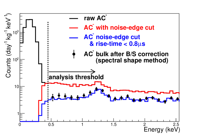
Figure 1: AC^- spectra of CDEX-1 experiment at various stages [12]: before performing noise-edge cut, after noise-edge cut, spectrum after noise-edge cut and event selection by $\tau$$<$0.7$\mu{s}$, spectrum after noise-edge cut and B/S correction of spectral shape method (described in Section 4) It shown that the noise-edge is around 350 eV, the analysis threshold in this article is set at 450 eV.

2 Anomalous Surface Events in pGe Detectors

The anomalous surface charge collection effect in pGe was noted in early literature [6]. Recent interest of adopting the pGe techniques in dark matter experiments gives rise to thorough studies [14, 15, 16].

The $n^{+}$ surface electrodes of pGe are fabricated by lithium diffusion and have a typical thickness of $\sim$1 mm [15, 18]. Electron-hole pairs produced at the surface (S) layer in pGe are subjected to a weaker drift field than those in the bulk volume (B). A fraction of the pairs will recombine while the residuals will induce signals which are weaker and slower than those originated in B. The S-events would therefore exhibit slower rise-time and partial charge collection compared to B-events. The charge collection efficiency as a function of the depth of the surface was recently measured and simulated [19]. The n-type point-contact germanium detectors, having micron-sized $p^{+}$ surface electrode due to boron-implantation, do not exhibit anomalous surface events [6].

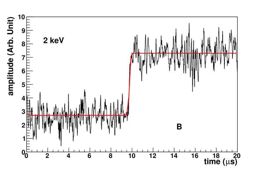
(a)

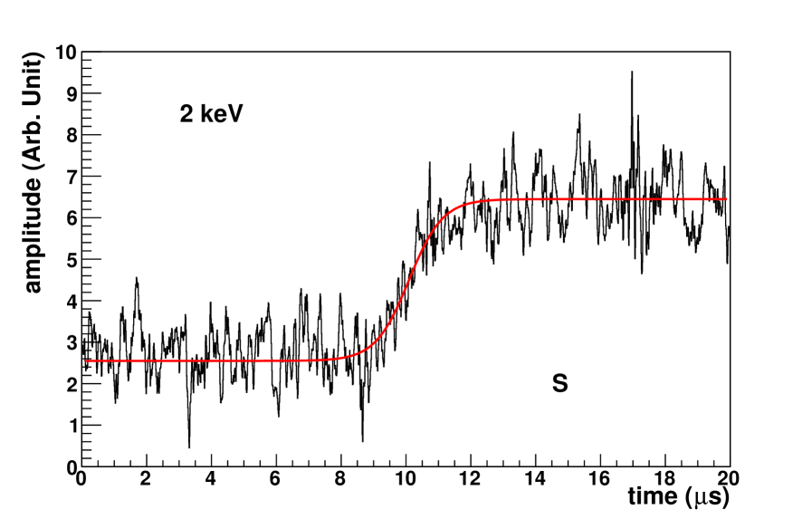
(b)

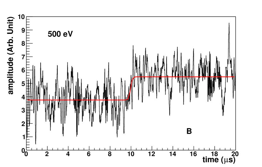
(c)

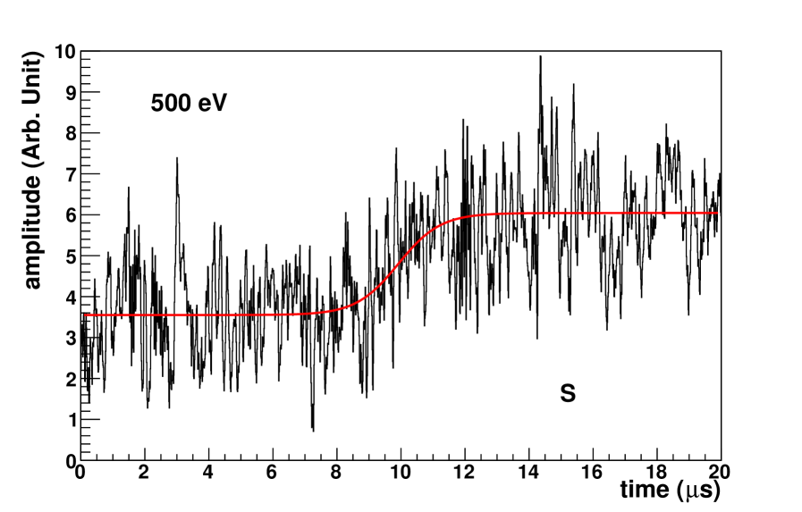
(d)

Figure 2: Amplitude versus time of typical pGe signals from CDEX-1 with (a) fast rise-time, from a 2 keV bulk event, (b) slow rise-time, from a 2 keV surface event, (c) fast rise-time, from a 0.5 keV bulk event and (d) slow rise-time, from a 0.5 keV surface event. The best-fit profiles from Eq. 1 are superimposed.

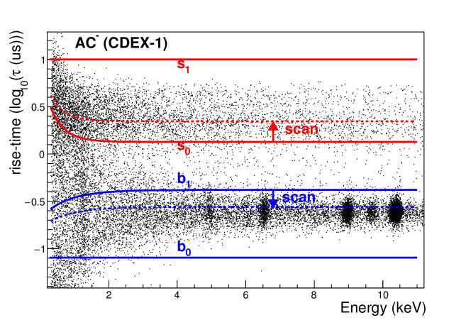
Figure 3: Rise-time versus energy scatter plot for the WIMP-induced candidate events based on $\rm{AC}^{-}$ selection in CDEX-1 data. The lines label $b_{0}$, $b_{1}$, $s_{0}$, $s_{1}$ are described in Section 5.2 and Section 6.3 for systematic checks.

Electronic signals are induced by the drifting charges. The signal rise-time ($\tau$) can be parametrized by the hyperbolic tangent function

$$\frac{1}{2}~{}{A_{0}}\times~{}\tanh(\frac{t-{t_{0}}}{\tau})~{}+~{}{P_{0}}~{}~{},$$ (1)

where ${A_{0}}$, ${P_{0}}$ and ${t_{0}}$ are the amplitude, pedestal offset and timing offset, respectively. Typical examples of B- and S-events, showing both their raw pulses and the fitted-profiles, at 2 keV and 0.5 keV, are illustrated in Figures 2a,b,c&d, respectively. A typical rise-time versus energy scatter plot is shown in Figure 3.

At high energy where S/N$>>$1, the fits are in excellent agreement with data indicating that Eq. 1 is an appropriate description of the rise-time of physics events. However, at low energy ($<$2 keV) where the signal amplitude is comparable to that of electronic pedestal noise, the B- and S-events could be falsely identified, giving rise to cross-contaminations. Software algorithms have to be applied to account for and correct these effects.

Typical pulses at energy near threshold are depicted in Figure 2c&d. The analysis threshold of 450 eV is well above the RMS of pedestal noise of 62 eV and measureable noise-edge of 350 eV, as shown in Figure 1. Assuming one exponentially decreasing noise contribution the fraction of noise events is $<$1% at 450 eV.

3 Rise-Time Uniformity

The validity of the software algorithms discussed in this article to differentiate bulk and surface events stands on the uniformity of $\tau$-distributions among both electronic and nuclear recoil events in describing the data to the desired level of accuracy.

Events produced by different particles (electrons, gammas, neutrons) exhibit similar bulk rise-time distributions in Ge detectors with the current generation of technology. Previous work indicated no difference of bulk rise-time distributions for $\gamma$-sources and nuclear recoil [20], and recent work reported that electron and nuclear events may differ in their rise-time by about $\sim$10 ns due to plasma effects [21], much faster than the typical Ge detectors rise-time of $\sim$1 ${\mu}s$. Differentiation of these signals are at the forefront of research, the success of which would represents a major advance in Ge-detector techniques and applications.

Bulk electron and nuclear recoil events are therefore indistinguishable from their rise-time distributions in Ge ionization detector [20]. Accordingly, rise-time distributions are the same at different B-regions while different depth in S-layers give different rise-time distributions due to the difference in diffusion time of electrons in the surface-inactive regions to the bulk-drifting volume [6, 12, 14]. The consequences of both are that the rise-time distributions are: (a) uniform for B-events for all sources while (b) different for S-events due to different event-depth distributions for sources of different energy.

Non-uniformity of surface rise-time distributions is corrected by calibration sources selection, as discussed in details in Section 6.1. The selection is data/experiment dependent, not universally applicable to all analysis.

The understanding of nature of rise-time distributions is beyond the scope in this analysis. An ab initio approach by simulation of behavior of particles in pGe and configuration of pGe would provide an alternative way to understand and address the B/S issue, though the current accuracies do not match the data-driven approaches discussed in this article.

4 Bulk-Surface Differentiation: Spectral Shape Method

The spectral shape method is a cut-based algorithm [14] developed to perform BSD for light WIMP searches with the CDEX-1 [11, 12] and TEXONO [13] data.

Two parameters have to be derived: the B-signal retaining and S-background suppression efficiencies, denoted by $\epsilon_{BS}$ and $\lambda_{BS}$, respectively. The efficiency-corrected “real” B- and S-rates $(B_{r},S_{r})$ are related to measured rates $(B_{m},S_{m})$ via:

$$B_{m}=\epsilon_{BS}B_{r}+(1-\lambda_{BS})S_{r}$$

$$S_{m}=\lambda_{BS}S_{r}+(1-\epsilon_{BS})B_{r},$$ (2)

with an additional unitary constrain of $B_{m}+S_{m}=B_{r}+S_{r}$.

The solutions of Eq. 2 are:

$$B_{r}=\frac{\lambda_{BS}B_{m}-(1-\lambda_{BS})S_{m}}{\epsilon_{BS}+\lambda_{BS}-1}$$

$$S_{r}=\frac{\epsilon_{BS}S_{m}-(1-\epsilon_{BS})B_{m}}{\epsilon_{BS}+\lambda_{BS}-1}.$$ (3)

Two components contribute to $B_{r}$($S_{r}$). The first positive term accounts for the loss of efficiency in the measurement of $B_{m}$($S_{m}$), while the second negative term corrects misidentification due to contamination effects. Both ($\epsilon_{BS},\lambda_{BS}$) factors should be properly accounted for in order to provide correct measurements of the energy spectra for bulk events.

In order to solve Eq. 2 for the two unknown parameters ($\epsilon_{BS},\lambda_{BS}$), at least two sources with different but known B- to S-event ratio are required. Four calibration sources (${}^{137}\rm{Cs}$, ${}^{241}\rm{Am}$, ${}^{57}\rm{Co}$ and ${}^{60}\rm{Co}$) [11, 12] were used in CDEX-1 analysis. The $B_{r}$ spectra of these sources were evaluated by full GEANT4 simulation, so that ($\epsilon_{BS}$, $\lambda_{BS}$) were derived having the corresponding measured $B_{m}$. The WIMP candidate data and ambient gamma background were then corrected by $\epsilon_{BS}$ and $\lambda_{BS}$.

However, there are several deficiencies with the spectral shape method:

1. Spectral shape assumption.
   Only sources with known spectral shape from simulations could be used as calibration data. In situ data like ambient background from $\gamma$-radioactivity do not contribute to calibration. This poses potential problems in long term data taking, such that data with external calibration source have to be taken at regular intervals and stability has to be assumed in between them.

   The $B_{r}$-spectra of calibration sources are evaluated from GEANT4 simulation, which depends on the detector structure and physics process subroutines adopted. In realistic data taking, there are additional contributions to $B_{m}$ due to cosmic-induced or ambient background which would introduce new error sources.

2. Normalization assumption.
   The spectra of $B_{m}$ and $B_{r}$ in calibration have to be normalized. The chosen scheme is to assume $\epsilon_{BS}$ and $\lambda_{BS}$ to be 1 [12, 14] (that is, perfect differentiation) at the high energy range of $\sim$2$-$4 keV for the various calibration data. This assumption, while reasonable, may introduce additional uncertainties.

3. Singularity problem.
   The solutions of Eq. 2 are undefined and the uncertainties becomes infinite when $\epsilon_{BS}+\lambda_{BS}$ approaches 1.

To address these drawbacks in performing BSD, we develop the ratio method to be discussed in the following sections.

5 Bulk-Surface Discrimination: Ratio Method

5.1 Concept and Formulation

Adopted data samples include calibration and in situ physics events, and are represented by index $i$. The goal of the analysis is to extract information on the B- and S-event distributions which are in general functions of $(E,\tau)$ and denoted as $N_{Bi}(E,\tau)$ and $N_{Si}(E,\tau)$, respectively. The relevant quantities for physics analysis are the real B- and S-rates which corresponds to, respectively,

$$B_{ri}(E)=\int_{all~{}\tau}N_{Bi}(E,\tau)d\tau~{}~{}~{}~{}{\rm and}~{}~{}~{}~{}~{}S_{ri}(E)=\int_{all~{}\tau}N_{Si}(E,\tau)d\tau~{}~{}.$$ (4)

In particular, $B_{ri}(E)$ would be the neutrino- and WIMP-induced candidate spectra where $i$ corresponds to the data sample surviving the electronic noise, cosmic-ray and anti-Compton veto selections.

One can write

$$N_{Bi}(E,\tau)=\beta_{i}(E)f_{B}(E,\tau)$$

$$N_{Si}(E,\tau)=\xi_{i}(E)f_{S}(E,\tau).$$ (5)

where $\beta_{i}(E)$ and $\xi_{i}(E)$ are $\tau$-independent scaling factors proportional to the B- and S-event rates. Evidence for independence of the rise-time distributions $f_{B}(E,\tau)$ and $f_{S}(E,\tau)$ from different particle interactions is discussed in Section 3.

The measured count rate of the $i^{th}$-sources as functions of $E$ and $\tau$ is therefore

$$N_{i}(E,\tau) = N_{Bi}(E,\tau)+N_{Si}(E,\tau)$$ (6)

$$= \beta_{i}(E)f_{B}(E,\tau)+\xi_{i}(E)f_{S}(E,\tau)~{}~{}.$$

To obtain the desired output of $N_{Bi}(E,\tau)$ and $N_{Si}(E,\tau)$, additional constraints must be provided to Eq. 6. For instance, modeling assumptions were made to $f_{B}(E,\tau)$ and $f_{S}(E,\tau)$ in the CoGeNT experiment [17], while the spectral shape method adopted in the TEXONO [14] and CDEX-1 [11, 12] analysis stands on having $\int{N_{Bi}(E,\tau)}d\tau$ values known by simulations for certain calibration sources.

For a collection of different sources with differing Bulk to Surface event ratios Eq. 6 can be used to find $N_{Bi}$ and $N_{Si}$ by $\chi^{2}$ minimization of the right hand-side of the equation, i. e., $\beta_{i}(E)f_{B}(E,\tau)+\xi_{i}(E)f_{S}(E,\tau)$

$$\chi^{2}(E,\tau)=\sum_{i}\frac{[\beta_{i}(E)f_{B}(E,\tau)+\xi_{i}(E)f_{S}(E,\tau)-N_{i}(E,\tau)]^{2}}{\Delta{N}_{i}(E,\tau)^{2}}~{}~{}.$$ (7)

The absolute values of $\beta_{i}(E)$ and $\xi_{i}(E)$ are not relevant to this analysis. The important values are $\beta_{i}(E)f_{B}(E,\tau)$ and $\xi_{i}(E)f_{S}(E,\tau)$.

In fact, we are free to choose $\beta_{i}(E)$ and $\xi_{i}(E)$, as long as they satisfy Eq. 5, which is equivalent to

$$\frac{N_{Bi}(E,\tau)}{N_{Bj}(E,\tau)}=\frac{\beta_{i}(E)}{\beta_{j}(E)}$$

$$\frac{N_{Si}(E,\tau)}{N_{Sj}(E,\tau)}=\frac{\xi_{i}(E)}{\xi_{j}(E)}.$$ (8)

This $\tau$-independent ratios are the basis of the ratio method.

If there exist uncontaminated B- and S- regions in $\tau$-space, then $\beta_{i}$ and $\xi_{i}$ can be chosen as

$$\beta_{i}(E)=\int_{b_{0}}^{b_{1}}{N_{Bi}(E,\tau)d\tau}{\approx}\int_{b_{0}}^{b_{1}}{N_{i}(E,\tau)d\tau}$$

$$\xi_{i}(E)=\int_{s_{0}}^{s_{1}}{N_{Si}(E,\tau)d\tau}{\approx}\int_{s_{0}}^{s_{1}}{N_{i}(E,\tau)d\tau}~{}~{},$$ (9)

as illustrated in Figure 4, with $\tau{\in}[b_{0},b_{1}]$ as boundaries of blue shadow box, and $\tau{\in}[s_{0},s_{1}]$ as boundaries of red shadow box. This choice of $\beta_{i}$ and $\xi_{i}$ satisfies Eq. 5 and 8, and provides the required scaling factors to solve Eq. 7. The boundary values ($b_{0}$, $b_{1}$, $s_{0}$ and $s_{1}$) are $E$-dependent in general. These can be selected within a range as long as they enclose the uncontaminated B- and S-regions.

At low energy near detector threshold, there are cross-contaminations between the B- and S-events. The algorithm to derive the scaling factors $\beta_{i}(E)$ and $\xi_{i}(E)$ in these regions is described in Section 5.2.

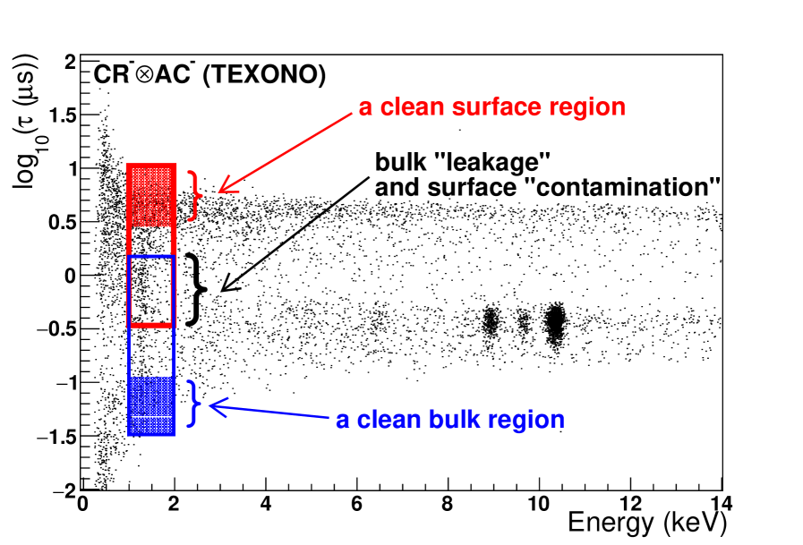
(a)

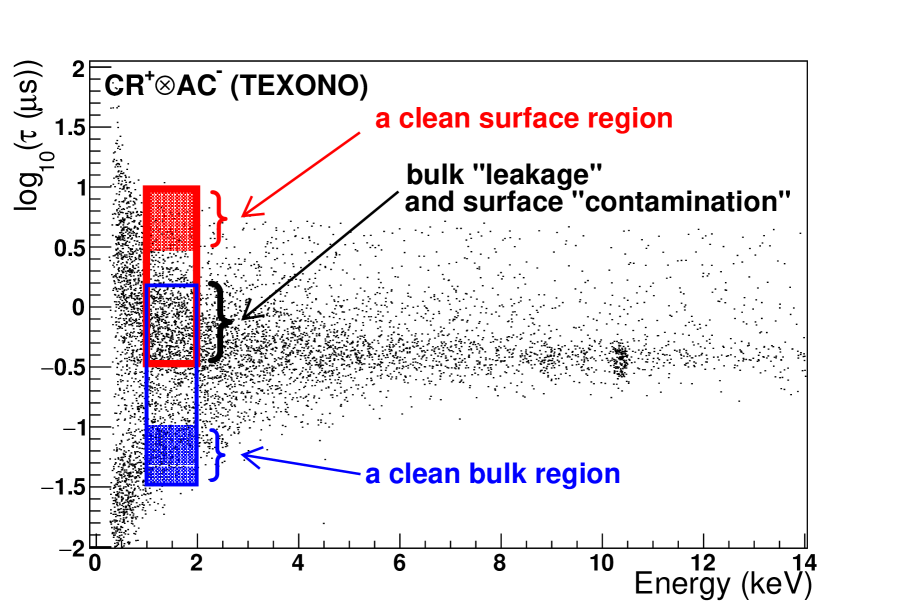
(b)

Figure 4: Rise-time versus energy plot for TEXONO data [13]: (a) anti-Compton and cosmic-ray vetoed samples (${\rm{CR}}^{-}\otimes{\rm{AC}}^{-}$), corresponding to neutrino- and WIMP-induced candidates, and (b) cosmic-ray coincident and anti-Compton vetoed samples (${\rm{CR}}^{+}\otimes{\rm{AC}}^{-}$), corresponding to cosmic-ray induced high-energy neutron interactions. The shaded blue and red regions correspond to the parameter space in B- and S-events, respectively, where there are no cross-contaminations among the two samples such that Eq. 8 is satisfied. These regions provide the solution of Eq. 7. The overlap of the two boxes correspond to regions with cross-contaminations.

In the limiting case of only two data samples (indexed as 0 and 1), the solution for $\beta_{0}(E)f_{B}(E,\tau)$ is:

$$\beta_{0}(E)f_{B}(E,\tau)=\frac{N_{1}(E,\tau)-[\xi_{1}(E)/\xi_{0}(E)]N_{0}(E,\tau)}{[\beta_{1}(E)/\beta_{0}(E)]-[\xi_{1}(E)/\xi_{0}(E)]}.$$ (10)

The solution is undetermined at $\beta_{1}/\beta_{0}=\xi_{1}/\xi_{0}$. That is, splitting a data set into two each having the same rise-time distribution profile would not provide a solution. The solutions for $\beta_{i}(E)f_{B}(E,\tau)$ and $\xi_{i}(E)f_{S}(E,\tau)$ exist only if at least two of the sources satisfy $\beta_{i}/\beta_{j}{\neq}\xi_{i}/\xi_{j}$. When all the sources have same $\beta_{i}/\beta_{j}$ and $\xi_{i}/\xi_{j}$, the statistic uncertainty will approach infinity (i. e., denominator of Eq. 10 approaches zero).

Discussions on statistical and systematic uncertainties of this algorithm are discussed in Section 6.3 in connection with the analysis on experimental data.

5.2 Cross-Contamination Regions

As illustrate in the $E<2~{}{\rm keV}$ range in Figure 3, there are contamination of S-events into $[b_{0},b_{1}]$ and of B-events into $[s_{0},s_{1}]$. In these domains, $\beta_{i}(E)$ and $\xi_{i}(E)$ could be derived by a successive approximation algorithm formulated as:

$$\beta^{(n)}_{i}(E)=\beta^{0}_{i}(E)-\int_{b_{0}}^{b_{1}}{\xi^{(n-1)}_{i}(E)~{}f^{(n-1)}_{S}(E,\tau)~{}d\tau}$$

$$\xi^{(n)}_{i}(E)=\xi^{0}_{i}(E)-\int_{s_{0}}^{s_{1}}{\beta^{(n-1)}_{i}(E)~{}f^{(n-1)}_{B}(E,\tau)~{}d\tau},$$ (11)

where $\beta^{0}_{i}(E)$ and $\xi^{0}_{i}(E)$ are initial guesses of scaling factors evaluated from Eq. 9, and $f^{(n-1)}_{B}(E,\tau)$ and $f^{(n-1)}_{S}(E,\tau)$ are results of minimizing Eq. 7 in the ${(n-1)}^{th}$-iteration.

At convergence for large $n$, the real B- and S-event rates for the $i^{th}$-samples are:

$$B_{ri}(E) = \int_{all~{}\tau}N_{Bi}(E,\tau)~{}d\tau=\int_{all~{}\tau}\beta^{(n)}_{i}(E)~{}f^{(n)}_{B}(E,\tau)~{}d\tau~{}~{}{\rm and}~{}~{}$$

$$S_{ri}(E) = \int_{all~{}\tau}N_{Si}(E,\tau)~{}d\tau=\int_{all~{}\tau}\xi^{(n)}_{i}(E)~{}f^{(n)}_{S}(E,\tau)~{}d\tau~{}~{},$$ (12)

respectively.

In practice, we adopted a 10-iteration calculation in this analysis. A systematic cross-check was performed with a 100-iteration calculation, where the difference is less than 0.01%.

6 Data Analysis

Published data from the CDEX-1 experiment [11, 12] were analyzed using the ratio method, and the results were compared with the results from the spectral shape method. Additional consistency checks were performed with TEXONO data [13, 14].

In both cases, the same event selections prior to BSD were made, including rejection of events due to electronic noise, and in coincidence with the cosmic-ray or anti-Compton detectors. In particular, events with extreme slow rise-time ($\tau>10~{}{\mu}s$) were discarded, since the contaminations of B-events to this region is negligible. These extremely large $\tau$ events were added to the S-samples to give the final $S_{ri}(E)$.

6.1 Rise-time Uniformity and Calibration Samples

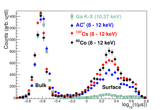
Figure 5: Rise-time distributions of Ga K-shell X-rays, $\rm{AC}^{+}$, ${}^{137}\rm{Cs}$ and ${}^{60}\rm{Co}$ events from CDEX-1 experiment at 8$-$12 keV.

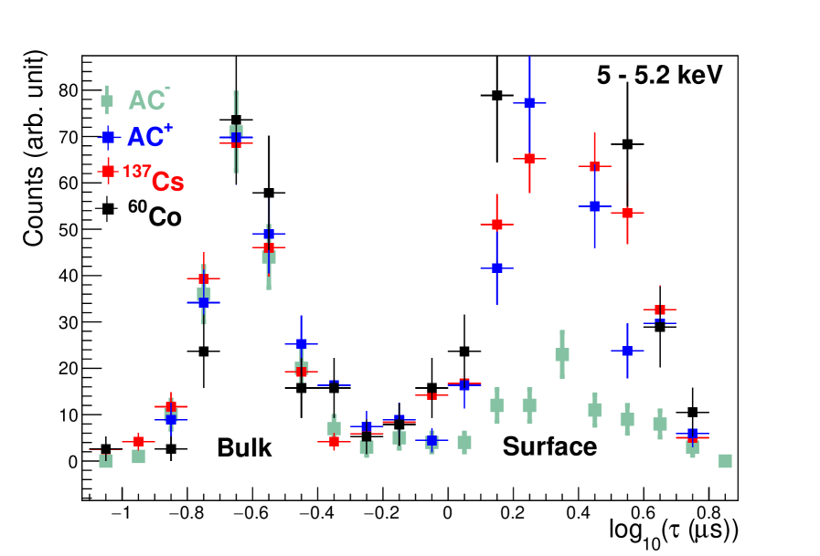
(a)

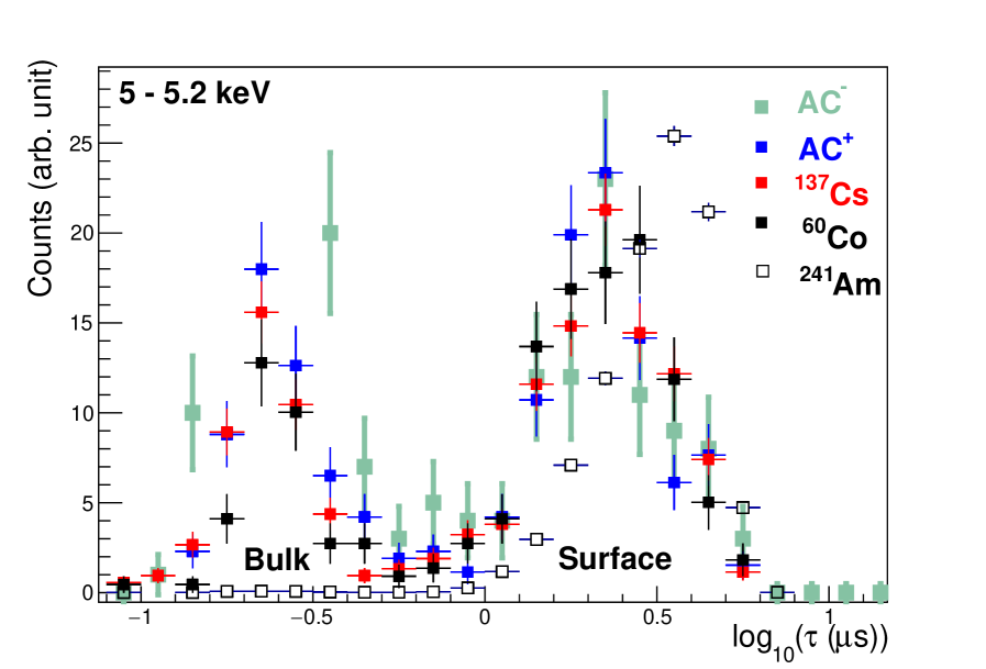
(b)

Figure 6: Rise-time distributions at 5$-$5.2 keV, (a) normalized to bulk counts and (b) normalized to surface counts show that B/S distributions for ${\rm{AC^{-}}}$, ${\rm{AC^{+}}}$, ${}^{137}{\rm{Cs}}$ and ${}^{60}{\rm{Co}}$ are consistent, with ${}^{241}{\rm{Am}}$ (which is not used in the analysis) for comparison. Note that at 5 keV, bulk and surface events are well separated.

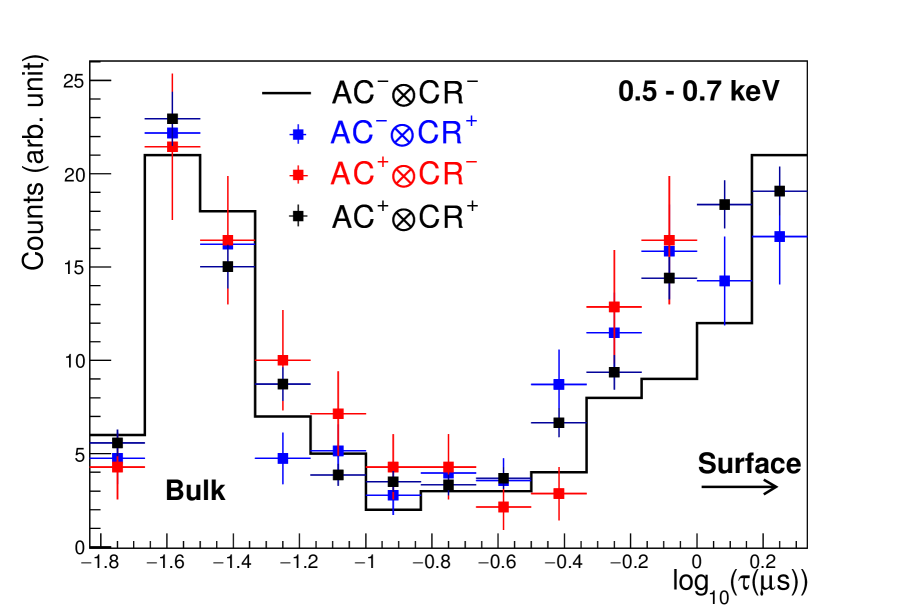
(a)

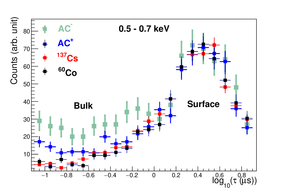
(b)

Figure 7: (a) Rise-time distributions of ${\rm{AC^{\pm}{\otimes}CR^{\pm}}}$ from TEXONO [13, 14] at 0.5$-$0.7 keV, showing that ${\rm{AC^{-}{\otimes}CR^{+}}}$ events are consistent with the others which are surface rich due to external $\gamma$-rays. (b) Rise-time distributions at 0.5$-$0.7 keV show that surface distributions for all sources are consistent.

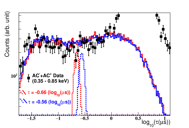
Figure 8: Comparison of rise-time distributions of $\rm{AC}^{-}+{AC}^{+}$ data in CDEX-1 (0.35$-$0.85 keV) with those from simulated pulses at two different rise-times shifted by 0.1 (${\rm{log_{10}({\mu}s)}}$). The dotted and solid lines correspond to those derived from amplitude of 10.37 keV and 0.6 keV, respectively, coupled with random pedestal noise.

	5$-$5.2 keV	5$-$5.2 keV	0.5$-$0.7 keV	0.5$-$0.7 keV	10.37 keV	0.5$-$0.7 keV
	surface	bulk	surface	bulk	bulk	bulk
$\tau$ range (${\rm{log_{10}({\mu}s)}}$)	0.1$-$0.45	-0.75$-$-0.5	0.2$-$0.8	-1.8$-$-1.2	simulation	simulation
				(TEXONO)
Mean of $\rm{AC}^{-}$	0.36	-0.63	0.46	-1.5	-0.46	-0.19
$\sigma$ of $\rm{AC}^{-}$	0.028	0.013	0.02	0.16	0.049	0.54
Deviations of mean	0.03	0.02	0.02	0.03	0.1†	0.008
† Input shift for simulation pulses.

Table 1: The mean and $\sigma$ of rise-time distributions for bulk and surface events at high (5.0$-$5.2 keV) and low (0.5$-$0.7 keV) energy, and the maximal deviations of different samples from the mean as in Figure 6&7. An additional estimate is made for the low energy bulk samples (rightmost column) from the differences in $\tau$ of the simulated pulses of Figure 8. The maximal deviations are adopted as input to one of the terms in the evaluation of systematic uncertainties in Table 2.

The validity of this analysis requires calibration source data with consistent rise-time distributions. These conditions are satisfied automatically for the B-samples at all energies, as discussed in Section 3 and shown in Figures 5, 6a and 7a.

As depicted in Figure 6b for the S-samples at keV energy, we selected those calibration sources which give consistent rise-times as the physics samples, all of which originate from high energy gamma-interactions. On the contrary, low energy gamma’s from ${}^{241}{\rm{Am}}$ which have severe attenuation at the surface layers cannot be used. The optimal selection of the calibration data is different for different experiments. For this analysis, samples from $\rm{AC}^{-}$, $\rm{AC}^{+}$, ${}^{137}{\rm{Cs}}$ and ${}^{60}{\rm{Co}}$ are selected for calibration of the CDEX-1 data [11, 12] discussed in Section 6.4, and from $\rm{CR}^{-}\otimes\rm{AC}^{-}$, $\rm{CR}^{+}\otimes\rm{AC}^{-}$, $\rm{CR}^{-}\otimes\rm{AC}^{+}$ and $\rm{CR}^{+}\otimes\rm{AC}^{+}$ of the TEXONO data [13] discussed in Section 6.5.

At low energies (below 1 keV for the data discussed in this article), resolution effects smear out the intrinsic rise-time differences for the S-events, such that the measured rise-time distributions are the same for all sources, as shown in Figures 7b and 8.

The uniformity of rise-time distributions and their independence to locations and nature of interactions are demonstrated for the selected calibration samples. The ${}^{137}{\rm{Cs}}$ and $\rm{AC}^{+}$ events are electron-recoils induced by $\gamma$-rays external to the detector and therefore have higher probability of located close to the surface. The Ga K-shell X-rays (10.37 keV) are also electron-recoils but due to cosmogenic activation inside the detector and are therefore uniformly distributed within the entire fiducial volume. The $\rm{CR}^{+}\otimes\rm{AC}^{-}$ samples select cosmic-ray induced high energy neutrons giving rise nuclear recoil events at the detector. Both the energy distribution (exponential rise towards low energy) and bulk-surface events ratio (uniformly distributed with detector) show these selected samples are neutron-rich [14]. By comparing with neutron flux measurement with a hybrid liquid scintillator detector [22] placed at the same location as the Ge-target, the fraction of nuclear recoils is about 99% [23]. The measured bulk-event rise-time distributions for these samples (${}^{137}{\rm{Cs}}$, $\rm{AC}^{+}$, Ga X-rays, $\rm{CR}^{+}\otimes\rm{AC}^{-}$) are all consistent with each other.

Gaussian fits are performed to derive the mean and root-mean-square (RMS) of the rise-time distributions. The $\rm{AC}^{-}$ samples are candidate events uncorrelated with other detector components and therefore the subjects of physics analysis. The deviations of various sources relative to the $\rm{AC}^{-}$ events are summarized in Table 1. The maximal shift of the mean is $\sim$ 1 RMS. This deviation matches the expectations due to measurement and statistical uncertainties, and has been taken in account in the consideration of systematic uncertainties to be discussed in Section 6.3.

Analysis on simulated pulses is performed to provide additional support to the rise-time independence. Rise-time of 10.37 keV Ga K-shell X-rays events were measured. Two event samples with $\tau$ at $\pm$ 1 RMS of the mean were extracted and added together to obtain their respective “averaged” pulse shape. These smoothed reference pulses were added to a large sample of random pedestal noise profiles. The measured rise-time of these simulated events are depicted in Figure 8. It shows two Gaussians with $\Delta\tau$ = 0.1 (${\rm{log_{10}({\mu}s)}}$). The same analysis was repeated with the reference pulses scaled to 0.6 keV instead. The measured rise-time distributions, also displayed in Figure 8, show broad profiles identical in both samples. As listed in Table 1, the corresponding shift of the means is less than the RMS, demonstrating that an artificial shift of intrinsic rise-time would produce no measureable effects at low energy, which is the crucial region of interest in BSD analysis. This further justifies the validity of the calibration samples selection.

6.2 Best-fit of Rise-time Distributions

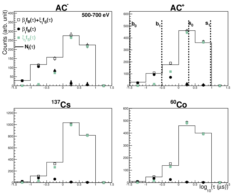
Figure 9: Best-fit results of Eq. 7 on CDEX-1 data, for $f_{B}(E,\tau)$ and $f_{S}(E,\tau)$ at $E=500$-$700~{}{\rm eV}$. The histogram $N_{i}(E,\tau)$ corresponds to the raw data, with $i~{}=~{}\{\rm{AC}^{-},\rm{AC}^{+},^{137}\rm{Cs},^{60}\rm{Co}\}$. The total $\chi^{2}$/dof for the combined data is 10.5/10.

Two in situ event samples are available in the CDEX-1 data: $\rm{AC}^{-}$ which are the WIMP candidate events and $\rm{AC}^{+}$ which are background due to ambient radioactivity. In addition, calibration data from ${}^{137}\rm{Cs}$ and ${}^{60}\rm{Co}$ sources were also taken. As discussed in Section 3, these data samples have similar $f_{B}(E,\tau)$ and $f_{S}(E,\tau)$ distributions at large $E$ where the BSD is distinct, but they also complement each other through having different B- and S-events ratios.

Contrary to the spectral shape method, the ratio method does not require assumption or simulation input on spectral shape. Accordingly, all four samples can contribute to BSD. Although two of these are in principle sufficient to provide solutions to Eq. 7, the information from all samples would provide redundancy and reduce uncertainties especially at low energy ($<$1 keV).

Best fit results for $f_{B}(E,\tau)$ and $f_{S}(E,\tau)$ at $E=500$-$700~{}{\rm eV}$ are depicted in Figure 9.

6.3 Uncertainties and Goodness-of-Fit

The sources and size of statistical and systematic uncertainties on a low and a high energy bins of the CDEX-1 $B_{ri}$ samples at the $i=\rm{AC}^{-}$ channel are summarized in Table 2. Standard error propagation techniques are used to evaluate the combined uncertainties of $B_{ri}$ and $S_{ri}$ for every $E$-bin.

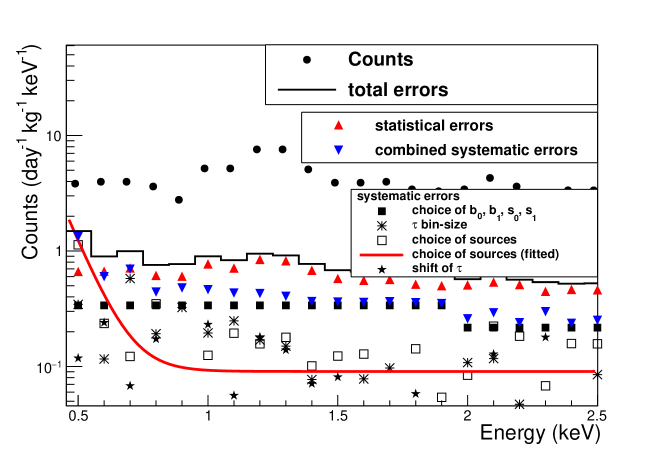
Figure 10: Distribution of count rates and their uncertainties of $B_{ri}(E)$ sample of CDEX-1 data for the $i={\rm AC^{-}}$ channel. The various contributions to both statistical and systematic errors are also shown. The threshold bin is with $E=450$$-$$550~{}{\rm eV}$. At low energy, the largest contribution comes from the choice of sources and the choice of $b_{0}$, $b_{1}$, $s_{0}$ and $s_{1}$, whereas errors are dominated by statistical errors at high energy.

There are three factors contributing to the statistical errors:

1. Errors at 1-$\sigma$ level on $f_{B}$ and $f_{S}$ are calculated from $\chi_{min}^{2}+1$ of Eq. 7 for each $(E,\tau)$-bin;

2. Errors of $\beta^{0}_{i}$ and $\xi^{0}_{i}$ for every $E$-bin;

3. Errors of correction terms of $\beta^{(n-1)}_{i}$ and $\xi^{(n-1)}_{i}$ in Eq. 11.

Energy	0.45$-$0.55 keV	0.55$-$0.65 keV
Counts and errors	3.83$\pm$0.66[stat]	3.99$\pm$0.67[stat]
(${\rm{day}}^{-1}$${\rm{kg}}^{-1}$${\rm{keV}}^{-1}$)	$\pm$1.23[sys]	$\pm$0.60[sys]
Systematic uncertainties:
(1) Choice of $b_{0}$, $b_{1}$, $s_{0}$ and $s_{1}$:	0.34	0.34
(2) $\tau$ bin-size:	0.35	0.12
(3) Choice of sources:	1.12	0.42
(4) Shift of $\tau$ by 0.02 (${\rm{log_{10}({\mu}s)}}$):	0.12	0.24
(5) Contribution of low energy $\gamma$:	$<$0.0028	$<$0.0028
(6) Non-zero counts at clean-bulk/surface:	$<$0.038	$<$0.038
(7) Iterations of $\beta_{i}(E)$, $\xi_{i}(E)$:	$<{\rm{10^{-4}}}$	$<{\rm{10^{-4}}}$

Table 2: The various contributions to the systematic uncertainties of $B_{r}$ of AC^- at two different energy bins.

The systematic uncertainties of the $E=450$$-$$550~{}{\rm eV}$ bin are displayed in Figure 10. Their derivations are discussed as follows, in which items 3-6 are related to possible non-uniformities of the rise-time pulse shape:

1. Choice of $b_{0}$, $b_{1}$, $s_{0}$, $s_{1}$.
   The ranges of [$b_{0}$, $b_{1}$] and [$s_{0}$, $s_{1}$] according to Figure 3 are reduced by 25%, and the maximum deviations in the results within a 2 keV bin are taken as systematic errors. Reduced ranges imply larger fluctuations in the count rates.

2. Choice of $\tau$ bin-size.
   Systematic effects are taken as deviations of results due to variations of bin-size, from half to twice the nominal one.

3. Choice of different combinations of calibration data.
   This is the largest contribution of systematic uncertainties at energy near threshold. Identical analysis were performed without ${\rm{AC^{+}}}$, ${}^{137}\rm{Cs}$ or ${}^{60}\rm{Co}$, one at a time. The systematic uncertainties are assigned from the best-fit function (the red curve of Figure 10) of the maximum deviations. The results remain mostly unchanged at high energy where bulk and surface events are well separated. However, at low energy, where B/S mixture is severe, the uncertainty of the B/S separation depends on the number of calibration sources. Removing sources increase uncertainties with strong energy dependence, as shown in Figure 10.

4. Deliberately shifting the mean rise-time of calibration events.
   The rise-time of ${\rm{AC^{-}}}$ is shifted by the amount allowed in Table 1, and the deviations of results are taken as systematic errors.

5. Extra low energy $\gamma$’s component at surface region.
   Surface rise-time distributions of high energy $\gamma$’s, e. g., ${\rm{AC^{+}}}$, ${}^{137}{\rm{Cs}}$ and ${}^{60}{\rm{Co}}$ resemble that of ${\rm{AC^{-}}}$. Sources that do not resemble ${\rm{AC^{-}}}$ can be represented by low energy $\gamma$’s from ${}^{241}{\rm{Am}}$ whose surface rise-time distributions at 5 keV is shown in Figure 6b.

   Upper bounds of their contributions to systematic uncertainties could be calculated by a simplified two components linear-fit to the surface region of ${\rm{AC^{-}}}$ at the high energy region:

   $$N_{{\rm{AC^{-}}}}(\tau)={\alpha}N_{{\rm{AC^{+}}}+^{137}{\rm{Cs}}+^{60}{\rm{Co}}}(\tau)+(1-\alpha)N_{{}^{241}{\rm{Am}}}(\tau).$$ (13)

   The best-fit results show that $(1-\alpha)$$=$7.1$\pm$8.4% (68% C. L.), which corresponds to deviation of $B_{r{\rm{AC^{-}}}}$ by $<$ 0.1 counts (${\rm{day}}^{-1}$${\rm{kg}}^{-1}$${\rm{keV}}^{-1}$) or $<$ 0.2% increasing in total errors at 450$-$550 eV.

6. Finite $f_{B}$ ($f_{S}$) counts at clean-surface (-bulk) region.
   In ideal cases, the $f_{B}(\tau)$ (or $f_{S}(\tau)$) solution should perfectly match with the rise-time distributions of the sources, and $f_{S}(\tau)$ (or $f_{B}(\tau)$) should be exactly zero in the clean-bulk (or clean-surface) region at 3$-$12 keV. Therefore, the finite $f_{B}$ ($f_{S}$) counts measurements can be served to quantify non-uniformities among chosen sources.

   Figure 11 depicts the best-fit results at 4$-$4.8 keV. Finite $f_{S}(\tau)$ counts at clean-bulk region (and $f_{B}(\tau)$ counts at clean-surface region) contributes to $<$ 0.24 counts (${\rm{day}}^{-1}$${\rm{kg}}^{-1}$${\rm{keV}}^{-1}$) of $B_{r{\rm{AC^{-}}}}$. These originates from statistical fluctuations and possible pulse-shape non-uniformity.

   At low energy, the finiteness originates from B/S contaminations and statistical fluctuations, as well as pulse-shape non-uniformity. That provides a measurement of upper bounds on the effects due to non-uniformity. At 500$-$700 eV, contribution of finite $f_{B}$ ($f_{S}$) counts is $<$ 0.39 ${\rm{day}}^{-1}$${\rm{kg}}^{-1}$${\rm{keV}}^{-1}$ of $B_{r{\rm{AC^{-}}}}$, equivalent to $<$ 2.7% increasing in total errors of $B_{r{\rm{AC^{-}}}}$.

7. Systematic uncertainties from the iterations of $\beta_{i}(E)$, $\xi_{i}(E)$ corrections are negligible.

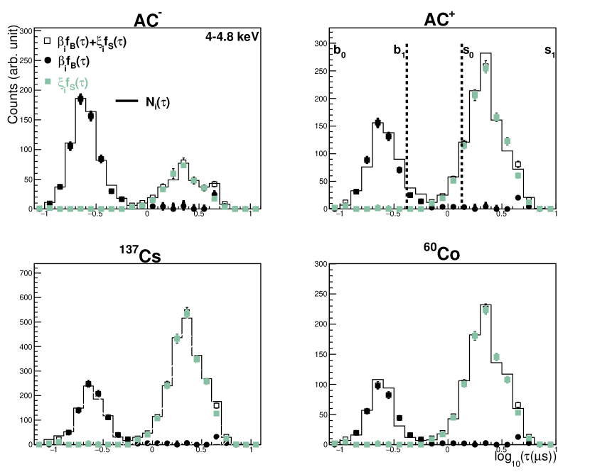
Figure 11: Best-fit results of Eq. 7 on CDEX-1 data, for $f_{B}(E,\tau)$ and $f_{S}(E,\tau)$ at $E=4$-$4.8~{}{\rm keV}$. The histogram $N_{i}(E,\tau)$ corresponds to the raw data, with $i~{}=~{}\{\rm{AC}^{-},\rm{AC}^{+},^{137}\rm{Cs},^{60}\rm{Co}\}$. A finer binning is used to demonstrate that $f_{B}$ is close to zero at clean-surface region (and vice versa). Small amount of non-zero $f_{B}$ counts at clean-surface region is caused by statistical non-uniformity. Nevertheless, those non-zero counts could serve as measurement of non-uniformity.

In addition, there are no indications from the literature and from measurements that there may be intrinsic pulse shape differences between high and low energy B-events. The data shows that even large differences in the Surface pulse shapes at high recoil energies between high and low-energy gamma sources are washed out at low recoil energy. It is therefore justified that residual differences in the B-event pulse shapes, if they exist, would be negligible at low energy.

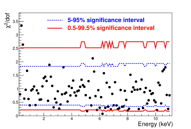
Figure 12: The goodness-of-fit ($\chi^{2}$/dof) derived through minimization of Eq. 7 on CDEX-1 data in Figures 9a, b, c, d. The threshold bin is with $E=450$$-$$550~{}{\rm eV}$ (350$-$450 ${\rm eV}$ is also shown) and every energy bin is independent. The related significant intervals are also displayed.

Combining both statistical and systematic uncertainties for every energy bin, the goodness of fit to Eq. 7 can be assessed via the $\chi^{2}$/dof values. The results are displayed in Figure 12. Degree of freedom at each energy bin is the total number of non-zero $\tau$-bins of all four sources subtracting off total non-zero $\tau$-bins of $f_{B}$ and $f_{S}$. The respective significant intervals are superimposed on Figure 12, indicating valid fit results and justifying that the four data samples share similar rise-time profiles in $f_{B}$ and $f_{S}$ above $\sim$550 eV for this data set [12].

6.4 Energy Spectra

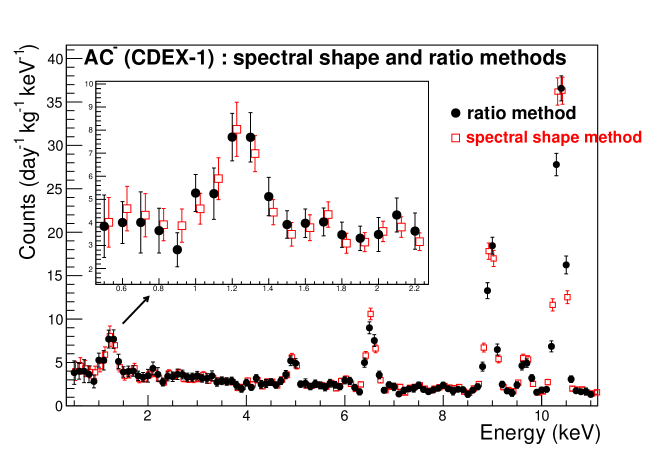
Figure 13: The CDEX-1 $B_{ri}(E)$ spectra for AC^- sample. Analysis is performed and results are compared with both spectral shape and ratio methods. The thresholds are 450 eV and 475 eV for the ratio and spectral shape methods, respectively. Systematic errors are included.

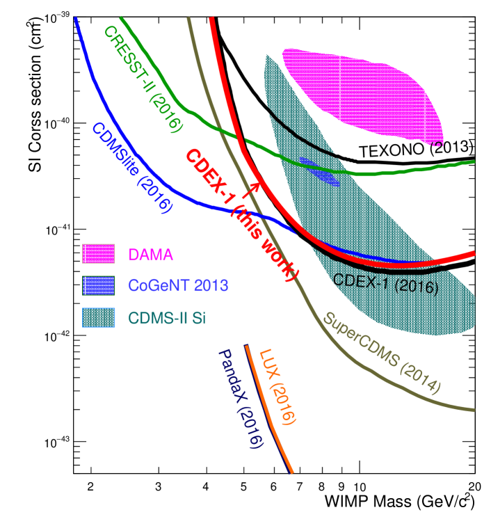
Figure 14: The WIMP-nucleon spin-independent cross-section exclusion plot, comparing results of the spectral shape method (CDEX-1 (2016)) and ratio method (CDEX-1 (this work)) from the CDEX-1 data. Also shown are 90% confidence upper limits from other benchmark results such as CDEX-1 (black) [11], CDMSlite (blue) [24], CRESST-II (dark green) [25], SuperCDMS (olive) [26], PandaX (dark blue) [27], and LUX (orange) [28], as well as allowed regions from DAMA (pink) [29, 30], CoGeNT (purple) [8] and CDMS II Si(teal) [31].

The CDEX-1 energy spectra $B_{ri}(E)$ at $i=\rm{AC}^{-}$ channel derived with both the spectral shape and ratio methods are depicted in Figure 13, indicating consistency among them. The figure also shows that all the internal X-ray peaks are correctly reconstructed. This is a non-trivial demonstration of validity of the ratio method, since every energy bin is processed independently of the others.

A comparison of the spin-independent WIMP-nucleon cross-section exclusion plot for both methods is shown in Figure 14, also indicating consistent results. The slight improvement with the ratio method at low mass ($<$6 GeV) originates from lower analyzable threshold (450 eV). The slight decrease in sensitivities at high mass is due to increased systematic uncertainties when the normalization assumption of the previous spectral method is no longer made.

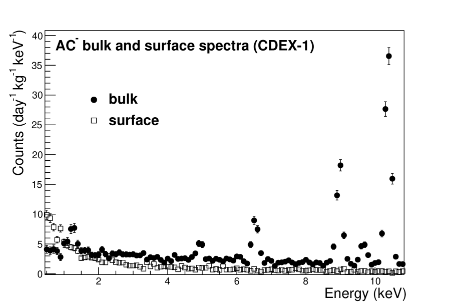
(a)

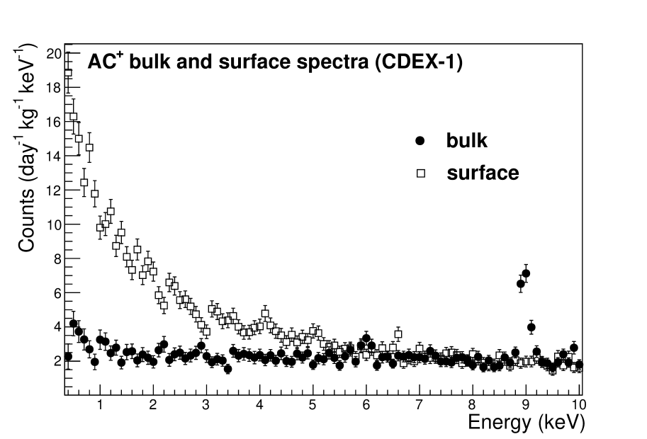
(b)

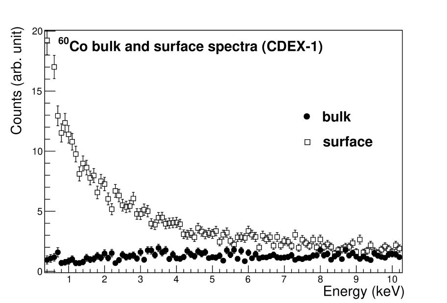
(c)

Figure 15: Bulk and surface spectra ($B_{ri}(E)$ and $S_{ri}(E)$, respectively) for (a) $\rm{AC}^{-}$, (b) $\rm{AC}^{+}$ and (c) ${}^{60}\rm{Co}$. All X-ray peaks are correctly assigned to bulk spectra, and all surface spectra show monotonic increase at low energy, as expected.

In addition to slower rise-time, the S-events are also characterized by incomplete charge collection, which manifests as spectra with monotonic increase at low energy, as verified in Figure 15 show that the $S_{ri}(E)$ spectra for $i=\{{\rm AC^{-}},{\rm AC^{+}},{\rm{}^{60}Co}\}$. In comparison, the $B_{ri}(E)$ of the same channels are flat, as expected from their origins of Compton scattering.

6.5 TEXONO data

Re-analyses of published data from the TEXONO experiment [13] were also analyzed with the ratio method. Unlike the procedures for CDEX-1 analysis discussed in Section 6.2, external calibration sources are not used. Instead, the analysis relies exclusive on all four categories of in situ event samples: $\rm{CR}^{-}\otimes\rm{AC}^{-}$, $\rm{CR}^{+}\otimes\rm{AC}^{-}$, $\rm{CR}^{-}\otimes\rm{AC}^{+}$ and $\rm{CR}^{+}\otimes\rm{AC}^{+}$ which combine physics candidate samples as well as events due to ambient $\gamma$-rays and cosmic high energy neutrons. As illustrated in Figure 16, consistent results have been achieved with the spectral shape method which used ${}^{241}\rm{Am}$ and ${}^{137}\rm{Cs}$ sources as well as the $\rm{CR}^{+}\otimes\rm{AC}^{-}$ data of n-type point-contact germanium detector [14].

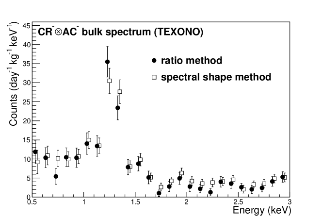
Figure 16: The $B_{ri}(E)$ spectra on the $\rm{CR}^{-}\otimes\rm{AC}^{-}$ channel from TEXONO data, with both spectral shape and ratio methods. The ratio method relies exclusively on in situ data in this case.

It can be seen from Figure 13 and 16 that both analysis methods on bulk-surface events identification with TEXONO [13] and CDEX-1 [11, 12] data, respectively, give rise to consistent results.

7 Summary and Prospects

The ratio method provides an alternative way to address the BSD problem in pGe. Results consistent with the previous spectral shape method are obtained, demonstrating its validity. Both methods are based on the assumption that the B- and S-events rise-time distributions (respectively, $f_{B}(E,\tau)$ and $f_{S}(E,\tau)$) are similar among the adopted data samples.

This feature is satisfied for B-events since nuclear- and electron-recoil events cannot be differentiated by their pulse shapes in germanium ionization detectors. The condition is also met for S-events at low near-threshold energy, the crucial energy range of interest, where the resolution smearing effects would dominate over intrinsic differences of their pulse shapes. At high energy, the requirement is matched with choice of calibration sources with consistent rise-time distributions as the physics samples. Systematic uncertainties as a result of such selection are evaluated, and then combined to derive the total uncertainties budget.

The most important merit of the ratio method is that the calibration can be achieved with in situ data, which can be neutrino- and WIMP-induced candidate events, cosmic-ray induced or ambient radioactivity background. This feature reduces or eliminates the dependence on external $\gamma$-ray sources for calibration purposes and therefore facilitates long-term data taking and operation of large multi-detector experiments. A drawback of the ratio method is the necessity to work in two-dimensional binning $(E,\tau)$, so that statistics have to be shared among many bins. The weight would be limited by the finite in situ counts in low background experiments. This gives rise to the choice for relatively large bin-size in 0.5 (${\rm{log_{10}({\mu}s)}}$) in the analysis.

Complete and accurate simulation of the Ge-detector behavior can provide complementary cross-checks to the calibration procedures and potentially improve on the systematic uncertainties. However, precise simulations of the rise-time distribution require many input parameters, some of which are not accurately known. In particular, the impurity levels and the leakage currents of the Ge-bulk crystal as well as details of resolution effects are crucial to the drift speed and hence the rise-time distributions. This is further complicated by possible time variations of the parameters. Simulation output at the current levels of sophistications do account for the qualitative behavior, but fall short of providing accurate quantitative descriptions of the measurement, as compared to the use of in situ calibration data discussed in this work. Refining in the physics parameters input and advancing on the simulation studies would be directions of future research.

8 Acknowledgment

This work is supported by the Academia Sinica Investigator Award 2011-15, contracts 103-2112-M-001-024 and 104-2112-M-001-038-MY3 from the Ministry of Science and Technology of Taiwan and the National Natural Science Foundation of China (Nos.11175099, 11275107, 11475117, 11475099 and 11475092) and the National Basic Research Program of China (973 Program) (2010CB833006) and the Tsinghua University Initiative Scientific Research Program No.20121088494.

References

- Luke et al. [1989] P. N. Luke, et al., Low capacitance large volume shaped-field germanium detector, IEEE Trans. Nucl. Sci. 36 (1989) 926.
- Barbeau et al. [2007] P. S. Barbeau, et al., Large-mass ultralow noise germanium detectors: performance and applications in neutrino and astroparticle physics, J. Cosmol. Astropart. Phys. 09 (2007) 009.
- Liu et al. [2017] S. K. Liu, et al., Constraints on Axion couplings from the CDEX-1 experiment at the China Jinping Underground Laboratory, Phys. Rev. D 95 (2017) 052006.
- Yue et al. [2004] Q. Yue, et al., Detection of WIMPs using low threshold HPGe detector, High Energy Phys. Nucl. Phys. 28 (2004) 877.
- Wong et al. [2006] H. T. Wong, et al., Research program towards observation of neutrino-nucleus coherent scattering, J. Phys. Conf. Ser. 39 (2006) 266.
- Soma et al. [2016] A. K. Soma, et al., Characterization and performance of germanium detectors with sub-keV sensitivities for neutrino and dark matter experiments, Nucl. Instr. Meth. Phys. Res. A 836 (2016) 67–82.
- Aalseth et al. [2011] C. E. Aalseth, et al., Results from a search for light-mass dark matter with a p-type point contact germanium detector, Phys. Rev. Lett. 106 (2011) 131301.
- Aalseth et al. [2013] C. E. Aalseth, et al., CoGeNT: A search for low-mass dark matter using p-type point contact germanium detectors, Phys. Rev. D 88 (2013) 012002.
- Aalseth et al. [2014] C. E. Aalseth, et al., Search for an annual modulation in three years of CoGeNT dark matter detector data, 2014. ArXiv:1401.3295.
- Zhao et al. [2013] W. Zhao, et al., First results on low-mass WIMPs from the CDEX-1 experiment at the China Jinping Underground Laboratory, Phy. Rev. D 88 (2013) 052004.
- Yue et al. [2014] Q. Yue, et al., Limits on light weakly interacting massive particles from the CDEX-1 experiment with a p-type point-contact germanium detector at the China Jinping Underground Laboratory, Phys. Rev. D 90 (2014) 091701(R).
- Zhao et al. [2016] W. Zhao, et al., Search of low-mass WIMPs with a p-type point contact germanium detector in the CDEX-1 experiment, Phys. Rev. D 93 (2016) 092003.
- Li et al. [2013] H. B. Li, et al., Limits on spin-independent couplings of WIMP dark matter with a p-type point-contact germanium detector, Phys. Rev. Lett. 110 (2013) 261301.
- Li et al. [2014] H. B. Li, et al., Differentiation of bulk and surface events in p-type point-contact germanium detectors for light WIMP searches, Astropart. Phys. 56 (2014) 1–8.
- Martin et al. [2012] R. D. Martin, et al., Determining the drift time of charge carriers in p-type point-contact HPGe detectors, Nucl. Instr. Meth. Phys. Res. A 678 (2012) 98–104.
- Aguayo et al. [2013] E. Aguayo, et al., Characteristics of signals originating near the lithium-diffused N+ contact of high purity germanium p-type point contact detectors, Nucl. Instr. Meth. Phys. Res. A 701 (2013) 176 – 185.
- Aalseth et al. [2015] C. E. Aalseth, et al., Maximum likelihood signal extraction method applied to 3.4 years of CoGeNT data, 2015. ArXiv:1401.6234v3.
- Jiang et al. [2016] H. Jiang, et al., Measurement of the dead layer thickness in a p-type point contact germanium detector, Chin. Phys. C 40 (2016) 096001.
- Ma et al. [2017] J. L. Ma, et al., Study of inactive layer uniformity and charge collection efficiency of a p-type point-contact germanium detector, Appl. Radiat. Isot. 127 (2017) 130–136.
- Baudis et al. [1998] L. Baudis, et al., High-purity germanium detector ionization pulse shapes of nuclear recoils, -interactions and microphonism, Nucl. Instr. Meth. Phys. Res. A 418 (1998) 348—354.
- Wei et al. [2016] W. Z. Wei, et al., Discrimination of nuclear and electronic recoil events using plasma effect in germanium detectors, J. Inst. 11 (2016) P07008.
- Singh et al. [2017] M. K. Singh, et al., Design and performance of a hybrid fast and thermal neutron detector, Nucl. Instr. Meth. Phys. Res. A 868 (2017) 109–118.
- Sonay [shed] A. Sonay, Characterization of neutron and high purity germanium detectors with advanced data acquisition system and measurement of neutron background at the Kuo-Sheng neutrino laboratory, M. Sc. thesis, Dokuz Eylül University, Turkey, 2018; to be published.
- Agnese et al. [2016] R. Agnese, et al., New results from the search for low-mass weakly interacting massive particles with the CDMS low ionization threshold experiment, Phys. Rev. Lett. 116 (2016) 071301.
- Angloher et al. [2016] G. Angloher, et al., Results on light dark matter particles with a low-threshold CRESST-II detector, Eur. Phys. J. C 76 (2016) 25.
- Agnese et al. [2014] R. Agnese, et al., Search for low-mass weakly interacting massive particles with SuperCDMS, Phys. Rev. Lett. 112 (2014) 241302.
- Tan et al. [2016] A. Tan, et al., Dark matter results from first 98.7 days of data from the PandaX-II experiment, Phys. Rev. Lett. 117 (2016) 121303.
- Akerib et al. [2017] D. S. Akerib, et al., Results from a search for dark matter in the complete LUX exposure, Phys. Rev. Lett. 118 (2017) 021303.
- Belli et al. [2011] P. Belli, et al., Observations of annual modulation in direct detection of relic particles and light neutralinos, Phys. Rev. D 84 (2011) 055014.
- Bernabei et al. [2010] R. Bernabei, et al., New results from DAMA/LIBRA, Eur. Phys. J. C 67 (2010) 39.
- Agnese et al. [2013] R. Agnese, et al., Silicon detector dark matter results from the final exposure of CDMS II, Phys. Rev. Lett. 111 (2013) 251301.