Second Harmonic Scattering as a
Probe of Structural Correlations in Liquids

Abstract

Second harmonic scattering experiments of water and other bulk molecular liquids have long been assumed to be insensitive to interactions between the molecules. The measured intensity is generally thought to arise from incoherent scattering due to individual molecules. We introduce a method to compute the second harmonic scattering pattern of molecular liquids directly from atomistic computer simulations, which takes into account the coherent terms. We apply this approach to large scale molecular dynamics simulations of liquid water, where we show that nanosecond second harmonic scattering experiments contain a coherent contribution arising from radial and angular correlations on a length-scale of $\lesssim 1$ nm - much shorter than had been recently hypothesized Shelton (2014). By combining structural correlations from simulations with experimental data Shelton (2014) we can also extract an effective molecular hyperpolarizability in the liquid phase. This work demonstrates that second harmonic scattering experiments and atomistic simulations can be used in synergy to investigate the structure of complex liquids, solutions and biomembranes, including the intrinsic inter-molecular correlations.

Nonlinear light scattering has been widely used to investigate aqueous interfaces, including suspensions of metallic or semiconducting nanoparticles, water droplets and biological membranes (for example, Refs. Eisenthal (2006); Roke and Gonella (2012); Gonella et al. (2012); Schürer et al. (2010); Butet et al. (2010); Russier-Antoine et al. (2010); Singh et al. (2013); Gonella et al. (2016); Smolentsev et al. (2016); Chen et al. (2015); Yan et al. (1998); Yang et al. (2001); Russier-Antoine et al. (2004); Kauranen et al. (1995)). In particular, second harmonic scattering (SHS), also commonly referred to as Hyper-Rayleigh scattering (HRS; the terms SHS and HRS are used interchangeably in this work), is especially sensitive to the molecular orientation of liquids at interfaces: there is a greater contribution to radiated second harmonic light arising from molecules at the interface, where inversion symmetry is broken, compared to those in the bulk, which is on average centrosymmetric. In bulk liquids the coherent term is usually assumed to be negligible and the measured signal is mostly interpreted in terms of fully incoherent scattering from individual molecules Terhune et al. (1965); Kauranen and Persoons (1996). Under this assumption, the SHS intensity of a solution can be expressed as a linear combination of the incoherent contribution of the solute and of that of the solvent. Using this approach the average hyperpolarizability of a molecule in solution can be estimated Clays and Persoons (1991).

This assumption stems from early work by Terhune et al., who neglected the coherent contribution to the intensity because the wavelength of the laser is much larger than the range of molecular correlations expected in a liquid Terhune et al. (1965). Although Bersohn and Maker later developed a theory to include coherent scattering due to structural correlations Bersohn et al. (1966); Maker (1970), these additional terms have been largely ignored in the interpretation of experiments. More recently, in a series of articles by Shelton et al., a sign of coherence has been reported from nanosecond HRS measurements on bulk liquids including water and acetonitrile Shelton (2000, 2002, 2005, 2014, 2015). A diverse range of possible origins was suggested for this coherence: a third order response arising from collective polar modes Shelton (2000), collective rotation of molecules Shelton (2002), the presence of ferroelectric domains Shelton (2005), coupling of rotations and translations in acoustic phonons extending up to 2000 nm Shelton (2014), or orientational correlations found in ideal isotropic homogeneous random vector fields Shelton (2015). Clearly SHS measurements contain information about the intermolecular structure of liquids although it is evident that no consensus has been reached on their origin (see e.g. Ref. Pounds and Madden (2007)) and their length scale. So far, experiments in bulk water have been interpreted by treating intermolecular correlations as fitting parameters Shelton (2014, 2015) and a framework to explicitly account for the correlations that give rise to coherent scattering in SHS experiments has not yet been developed. Recent elastic femtosecond SHS measurements from ionic solutions have shown that several different electrolytes induce long-range orientational correlations in water, starting at concentrations as low as 10 $\mu$M Chen et al. (2016). The strong dependence on isotopic composition also suggests a link between these observations and the H-bond network of water.

The liquid-phase hyperpolarizability plays a crucial role in the interpretation of SHS experiments. Measurements have often been analyzed using a molecular non-linear response tensor of water obtained from quantum chemical calculations Gubskaya and Kusalik (2001). However, the model that underlies the evaluation of of the hyperpolarizability in Ref. Gubskaya and Kusalik (2001) described the surroundings of a water molecule by three point charges, which does not take into account the many complex molecular environments that can be found in liquid water Gasparotto et al. (2016).

In this work we present a method to compute the SHS intensity directly from atomistic computer simulations, including both the incoherent and the coherent contributions. This framework is used to calculate the angular scattering pattern from large-scale force-field molecular dynamics (MD) simulations of liquid water. We show that quantitative agreement with nanosecond HRS experiments Shelton (2014) cannot be achieved by using the values of molecular hyperpolarizability often used to interpret experiments, Gubskaya and Kusalik (2001) obtained with Møller-Plesset perturbation theory expanded up to the fourth order (MP4). We find instead that it is possible to obtain satisfactory agreement by combining the correlations obtained from simulations with an effective liquid phase molecular hyperpolarizability, used as a fitting parameter. The values obtained for this hyperpolarizability can be used to provide a more quantitative interpretation of other SHS experiments. By computing explicitly the correlations that contribute to the SHS signal, we can also gather insight into the length scales that are most relevant for these experiments.

We begin by introducing the general expression for the SHS intensity $I(\mathbf{q},\mathbf{u},\mathbf{v})$ for an ensemble of $N$ molecules at a scattered wave-vector $\mathbf{q}$ and with the polarization directions of the incoming and outgoing beams defined by the vectors $\mathbf{u}$ and $\mathbf{v}$:

$$I(\mathbf{q},\mathbf{u},\mathbf{v})\propto N^{-1}\left\langle\left|\sum_{\alpha}\beta(\alpha,\mathbf{u},\mathbf{v})e^{\mathrm{i}\mathbf{q}\cdot\mathbf{r}_{\alpha}}\right|^{2}\right\rangle,$$ (1)

where the brackets indicate a time average over uncorrelated configurations and $\beta(\alpha,\mathbf{u},\mathbf{v})$ is the component of the hyperpolarizability of a scattering unit $\alpha$ in the laboratory reference frame (L) projected onto the polarization direction of the incoming ($\mathbf{u}$) and outcoming ($\mathbf{v}$) beams, i.e. $\beta(\alpha,\mathbf{u},\mathbf{v})=\sum_{LMN}\beta^{\textrm{L}}_{LMN}(\alpha)v_{L}u_{M}u_{N}$, and the proportionality constant can be found in Ref. Bersohn et al. (1966). A schematic of the geometric setup is shown in the Supporting Information (SI) in Fig. S1. Eq. 1 can be decomposed into the sum of an incoherent term and of a coherent term respectively Bersohn et al. (1966):

$$\begin{split}&I(\mathbf{q},\mathbf{u},\mathbf{v})\propto N^{-1}\left\langle\sum_{\alpha}\beta(\alpha,\mathbf{u},\mathbf{v})^{2}\right\rangle+\\ &N^{-1}\left\langle\sum_{\alpha}\sum_{\alpha^{\prime}\neq\alpha}\beta(\alpha,\mathbf{u},\mathbf{v})\beta(\alpha^{\prime},\mathbf{u},\mathbf{v})e^{[\mathrm{i}\mathbf{q}\cdot(\mathbf{r}_{\alpha}-\mathbf{r}_{\alpha^{\prime}})]}\right\rangle.\end{split}$$ (2)

The hyperpolarizability in the laboratory frame $\beta^{\textrm{L}}_{LMN}$ can be obtained by applying the rotations $\beta^{\textrm{L}}_{LMN}=\sum_{abc}\beta^{\textrm{M}}_{abc}c_{aL}c_{bM}c_{cN}$, with $\beta^{\textrm{M}}_{abc}$ being the molecular hyperpolarizability in the molecular frame and $c_{iI}$ the projection of the $i^{\rm th}$ unit vector in the molecular frame on the $I^{\rm th}$ unit vector in the lab frame. In the following we assume that $\beta^{\textrm{M}}_{abc}$ can be expressed as an effective molecular hyperpolarizability $\left<\beta^{\textrm{M}}_{abc}\right>$.

As previously discussed, in bulk liquids the coherent term in Eq. 2 – which describes the interference between the waves scattered by two molecules – would average to zero if the instantaneous relative orientation of different molecules were completely random, and is often assumed to be negligible compared to the incoherent term Eisenthal (2006); Terhune et al. (1965); Maker (1970); Clays and Persoons (1991) In order to test this assumption, we developed a framework to explicitly evaluate Eq. 1 for MD simulations. We applied this framework to MD simulations of liquid water involving about 260,000 molecules, using a cubic simulation box with a side of 20 nm. Simulations were performed with the GROMACS code v.5.0.4 Abraham et al. (2015), using the rigid TIP4P/2005 water model Abascal and Vega (2005). The equations of motion were integrated in the NVT ensemble using the velocity Verlet algorithm for 20 ns with a 2 fs timestep. Temperature control was achieved using the stochastic velocity rescaling thermostat Bussi et al. (2007), with a target temperature of 300 K. Full details of the computational setup can be found in the Supporting Information. We performed extensive tests on the setup to ensure that it was insensitive to finite size effects and the type of force-field used.

Fig. 1 shows the ratios of the SHS intensities of bulk water reported by Shelton in Ref. Shelton (2014) using nanosecond experiments at different polarization combinations as a function of the scattering angle ($\theta$) and as computed in this work from the analysis of our MD simulations. The convention used for the polarization combinations follows Ref. Chen et al. (2016) and references therein. Light polarized parallel to the scattering plane is denoted by P and light polarized perpendicular to the scattering plane is denoted by S. A polarization combination is specified as XYY, with X (= P or S) the polarization of the outgoing beam and Y (= P or S) that of the incoming beam. Fig. 1(a) illustrates the intensity ratios obtained from our simulations under the assumption of purely incoherent scattering. We use the constant hyperpolarizability from Ref. Gubskaya and Kusalik (2001), computed using MP4 and modelling a liquid-like environment by placing point charges in a geometry resembling the first solvation shell. Despite its simplicity, this model has been used in several studies of the hyperpolarizability of water Ward et al. (2013); Sonoda et al. (2005). It can be seen that a model for the intensity assuming only incoherent scattering completely fails to account for the qualitative features of the experimental curves, which show an asymmetry with respect to 90 degrees and a varying $I_{\text{SPP}}/I_{\text{PSS}}$ ratio.

We then proceed to compute the intensity with the full Eq. 1, using the $\left<\beta^{\text{M}}_{abc}\right>$ elements from Ref. Gubskaya and Kusalik (2001). As shown in Fig. 1(b), the functional form of the plot extracted from the simulation is markedly different from that of Fig. 1(a) and reproduces the main features of the experimental curves. However, the computed ratios show a clear quantitative difference from the experimental ratios. Rather than trying to refine the evaluation of this effective hyperpolarizability Sonoda et al. (2005); Sylvester-Hvid et al. (2004); Kongsted et al. (2004), one could extract the molecular correlations from the atomistic simulation, and verify whether the experimentally measured intensities can be reproduced by using the values of $\left<\beta^{\text{M}}_{abc}\right>$ as fitting parameters.

In order to investigate this point, we reformulate Eq. 1 in a form that separates intermolecular correlations and the tensor elements of the constant effective molecular hyperpolarizability $\langle\beta^{\textrm{M}}_{abc}\rangle$ in the liquid phase. We introduce the sixth-order tensor $W_{abcdef}(\mathbf{q},\mathbf{u},\mathbf{v})=N^{-1}\sum_{\alpha,\alpha^{\prime}}S^{*}_{abc}(\mathbf{q},\mathbf{r}_{\alpha},\mathbf{u},\mathbf{v})S_{def}(\mathbf{q},\mathbf{r}_{\alpha^{\prime}},\mathbf{u},\mathbf{v})$, where,

$$S_{abc}(\mathbf{q},\mathbf{r}_{\alpha},\mathbf{u},\mathbf{v})=\sum_{LMN}c_{aL}v_{L}c_{bM}u_{M}c_{cN}u_{N}\exp{(\mathrm{i}\mathbf{q}\cdot\mathbf{r}_{\alpha})}.$$ (3)

$W_{abcdef}(\mathbf{q},\mathbf{u},\mathbf{v})$ includes both the single-molecule term giving rise to incoherent scattering and the coherent contribution due to the intermolecular radial and angular correlations. Inserting this expression into Eq. 1 we obtain,

$$I(\mathbf{q},\mathbf{u},\mathbf{v})\propto\sum_{abcdef}\left\langle\beta^{\textrm{M}}_{abc}\right\rangle\left\langle\beta^{\textrm{M}}_{def}\right\rangle\left\langle W_{abcdef}(\mathbf{q},\mathbf{u},\mathbf{v})\right\rangle.$$ (4)

Because SHS experiments are performed at a value of $q$ of the order of $10^{-2}$ nm^-1, which is too small to be probed in simulations, we extrapolate $\left<W_{abcdef}(\mathbf{q},\mathbf{u},\mathbf{v})\right>$ to the $q\rightarrow 0~{}\text{nm}^{-1}$ limit (see SI). Having separated the expression for the intensity into the effective molecular hyperpolarizability and the structural correlation term $\langle W_{abcdef}(\mathbf{q},\mathbf{u},\mathbf{v})\rangle$, it is possible to use Eq. 4 to determine the value of $\langle\beta^{\textrm{M}}_{abc}\rangle$ that best matches experiments. The $\left<\mathbf{W}(\mathbf{q},\mathbf{u},\mathbf{v})\right>$ tensor needs to be computed only once, and weighted with tentative values of the hyperpolarizability tensor to find the best fit. Under nonresonant conditions Giordmaine (1965), and under the assumption that each water molecule in the condensed phase has $C_{2v}$ symmetry, there are only three independent components of the molecular hyperpolarizability tensor, i.e. $\beta^{\textrm{M}}_{zxx}$, $\beta^{\textrm{M}}_{zyy}$ and $\beta^{\textrm{M}}_{zzz}$. One value of the three elements of the hyperpolarizability is linearly dependent on the other two because most of the time, intensity ratios are extracted from SHS experiments, rather than the bare intensities.

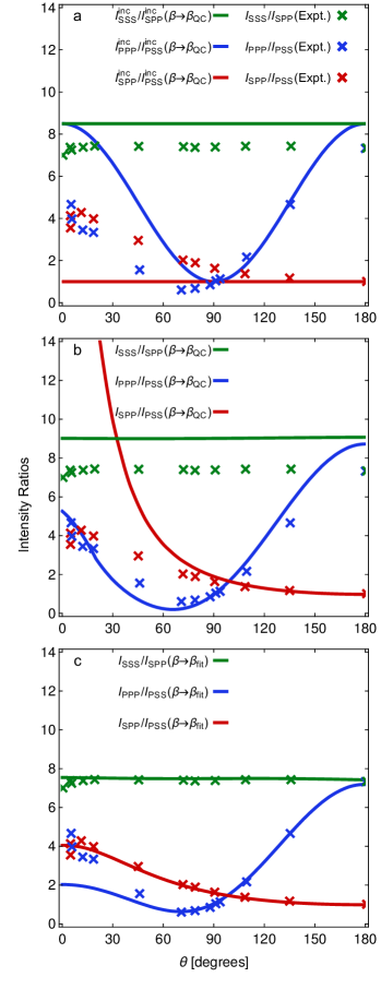
Figure 1: SHS intensity ratios of bulk water for different polarization combinations as a function of the scattering angle $\theta$ computed from MD (solid lines) and as measured by Shelton in Ref. Shelton (2014) (crosses). Intensity ratios with the molecular hyperpolarizability of H₂O in the liquid from Ref. Gubskaya and Kusalik (2001) (i.e. $\beta\rightarrow\beta_{\rm QC}$) and (a) assuming incoherent scattering, (b) including also the coherent contribution. (c) Ratios obtained from Eq. 4 including both the incoherent and the coherent contributions and where the molecular hyperpolarizability has been fitted to experiment, i.e. $\beta\rightarrow\beta_{\rm fit}$. The nanosecond HRS experimental data is reproduced with permission from the American Institute of Physics from Ref. Shelton (2014).

With these hypotheses in place, Fig. 2 shows the error ($\chi^{2}$) of the fit to the experimental data of Ref. Shelton (2014) as a function of $\langle\beta^{\textrm{M}}_{zxx}\rangle/\langle\beta^{\textrm{M}}_{zzz}\rangle$ and $\langle\beta^{\textrm{M}}_{zyy}\rangle/\langle\beta^{\textrm{M}}_{zzz}\rangle$. This plot can be used to ascertain the quality of a given model to compute the effective molecular hyperpolarizability in the condensed phase. For instance, the values of the molecular hyperpolarizabilities in the model of Ref. Gubskaya and Kusalik (2001) (the square symbol) give a much larger $\chi^{2}$ compared to the best estimate obtained by our fitting procedure (the circle symbol). It can also be seen that the parameter space of $\langle\beta^{\textrm{M}}_{zxx}\rangle/\langle\beta^{\textrm{M}}_{zzz}\rangle$ and $\langle\beta^{\textrm{M}}_{zyy}\rangle/\langle\beta^{\textrm{M}}_{zzz}\rangle$ that results in a small error is rather broad (see the orange region with $\chi^{2}<8$ in Fig. 2). Combining the data of Ref. Shelton (2014) with that of other experiments, e.g. on electrolyte solutions Chen et al. (2016), might allow one to narrow down the uncertainty on $\langle\beta^{\textrm{M}}_{abc}\rangle$. Fig. 1(c) shows directly the agreement between the measured intensity ratio and the results obtained from Eq. 4 using our best estimate for $\langle\beta^{\textrm{M}}_{abc}\rangle$, combined with the structural intermolecular correlations obtained from the MD trajectories. The reason for the discrepancy between the experimental and the simulated intensity ratios in Fig. 1(b) can thus be ascribed to the different value used for the effective hyperpolarizability. Although Fig. 1(c) agrees well with experiments, the agreement is not perfect at low scattering angles. The underlying reason is most likely the fact that the scattering plane becomes ill-defined as $\theta\rightarrow 0$, because the two vectors defining this plane ($\mathbf{k}_{\rm in}$ and $\mathbf{k}_{\rm out}$, as defined in the SI) become collinear in this limit.

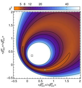
Figure 2: Contour plot of the mean standard error of the simulated intensity ratios from the experimental data ($\chi^{2}$) as a function of the independent components of the effective hyperpolarizability of water in the liquid phase. The circle and the square symbol indicate the values of the hyperpolarizabilities that give the minimum in the error and those computed in Ref. Gubskaya and Kusalik (2001), respectively.

Fig. 3 provides further insight into the correlations probed by SHS experiments. Fig. 3(a) shows a schematic of the experimental system, including for simplicity only a pair of molecules. SHS probes the correlations between projections of unit vectors in the molecular frame onto those of the laboratory reference frame for a given orientation of $\mathbf{q}$ and combination of $\mathbf{u}$ and $\mathbf{v}$. Fig. 3(a) thus provides a pictorial representation of Eqs.3 and 4. Different components of the $\left<\mathbf{W}(\mathbf{q,\mathbf{u},\mathbf{v}})\right>$ tensor report on complex combinations of radial and angular correlations. As a concrete example, $\langle W_{zzzzzz}\rangle$ for the SSS polarization combination, taking an experimental setup in which $\mathbf{q}$ lies in the $XY$ plane, is given explicitly by $\langle\sum_{\alpha,\alpha^{\prime}}c_{zZ}^{3}(\alpha)c_{zZ}^{3}(\alpha^{\prime})e^{i\mathbf{q}\cdot\left(\mathbf{r}_{\alpha}-\mathbf{r}_{\alpha^{\prime}}\right)}\rangle$, which involves the pair correlation function of the cube of the molecular dipole’s component in the direction of the laboratory $Z$ axis. Fig. 3(b) shows the effect of these correlations on three components of $\left<\mathbf{W}(\mathbf{q,\mathbf{u},\mathbf{v}})\right>$ as a function of wavevector. In the limit as $q\rightarrow 0$ there is a significant coherent contribution, which is a hallmark of intermolecular correlations.Bersohn et al. (1966) It can be seen that in this limit $\langle W_{zzzzzz}\rangle$ takes the largest value, while $\langle W_{zxxzxx}\rangle$ and $\langle W_{zyyzyy}\rangle$ are about 8 times smaller. This reflects the fact that the correlations between the water dipoles are stronger than those between the $x$ and $y$ molecular axes.

In the limit as $q\rightarrow 0$, $\left<\mathbf{W}(\mathbf{q,\mathbf{u},\mathbf{v}})\right>$ reports on the magnitude of the correlations integrated over all distances. By computing the value of $\left<\mathbf{W}(\mathbf{q,\mathbf{u},\mathbf{v}})\right>$ at finite $q$ we can quantify the length scale that gives the largest contribution to the SHS signal. As shown in Figure 3(b), $\langle W_{zzzzzz}\rangle$ converges to the incoherent limit, oscillating with a period of about 20 nm^-1, which corresponds to a strong contribution from correlations within the first and second solvation shell of each water molecule. This is shown in more detail by the Fourier transform of $\left<W_{zzzzzz}(q)\right>$ into the spatial domain, given in Fig. 3(c). The pair correlation function shown in the figure presents two pronounced peaks, corresponding to the first two solvation shells, and a decays to zero within $\sim 1$ nm. Therefore, the largest contribution to $\left<W_{zzzzzz}(q\rightarrow 0)\right>$ arises from pairs of molecules within the first couple of solvation shells, while long-distance tails give a negligible contribution. Correlations beyond a few nm are not crucial, as is clear from Fig. S2, where it is shown that the intensity ratios differ by a few percent when using a 5 nm simulation box compared to a 20 nm box. The SHS patterns of Shelton Shelton (2014) have been given a number of different interpretations, all of which involve the role of long-range correlations. Although intermolecular correlations on longer scales may be present, as observed in MD simulations of neat water Zhang and Galli (2014) and in SHS experiments (as well as MD simulations) of electrolyte solutions Chen et al. (2016), SHS measurements in neat water can be rationalized in terms of short-range correlations.

Fig. 3(b) focuses on an experimental setup that is particularly simple to interpret. However, $\left<\mathbf{W}(\mathbf{q,\mathbf{u},\mathbf{v}})\right>$ captures all of the correlations that are relevant for an SHS experiment. In the SI (see Figs. S4 and S5) we show the dependence of various tensor elements on the scattering angle and for different polarization combinations. Depending on the geometry of the experiment and the values of $\left<\mathbf{\beta}_{abc}^{\text{M}}\right>$, different measurements probe different combinations of molecular correlations. Based on this observation, it is possible to design experiments that are particularly sensitive to a given kind of correlation. For instance, with PPP polarization, $\theta\approx 0$ and $\theta\approx 180^{\circ}$ give the strongest coherent contribution, which is at odds with previous suggestions that measurements should be performed at $\theta=90^{\circ}$. Terhune et al. (1965)

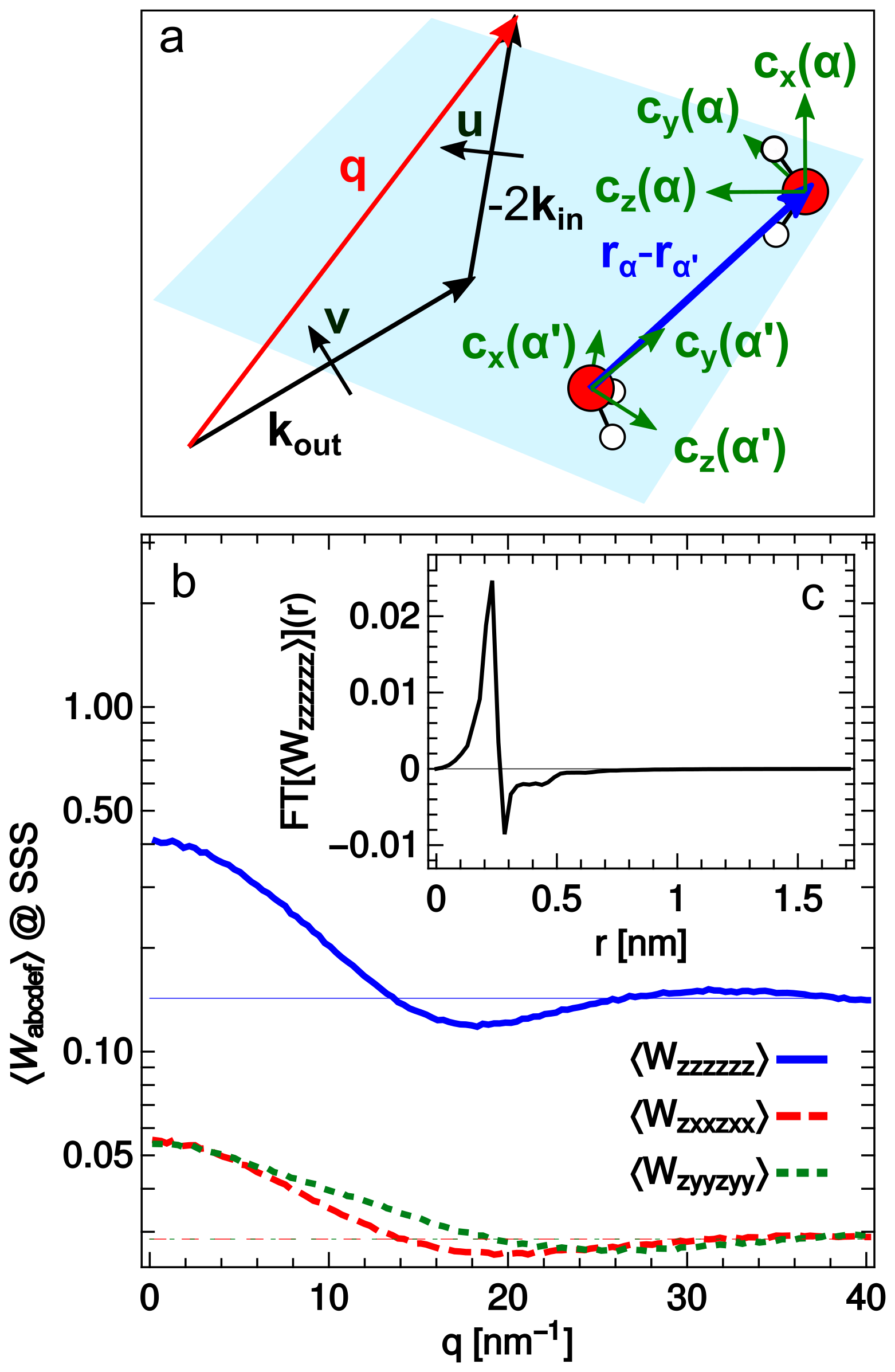
Figure 3: The role of angular and radial correlations in determining the SHS intensity. (a) Schematic of the SHS system in an arbitrary geometry including for simplicity only a pair of molecules, where $\mathbf{q}$, $\mathbf{k}_{\mathrm{in}}$, $\mathbf{k}_{\mathrm{{out}}}$ $\mathbf{u}$ and $\mathbf{v}$ define the experimental setup, while the $c$ vectors are the unit vectors of molecule $\alpha$ and $\alpha^{\prime}$ in their respective reference frames. (b) Wave vector dependence of $\langle W_{zzzzzz}\rangle$, $\langle W_{zxxzxx}\rangle$ and $\langle W_{zyyzyy}\rangle$ tensor elements in the SSS polarization (thin lines are the incoherent parts of these tensors). (c) Fourier transform of $\langle W_{zzzzzz}\rangle(q)$ demonstrating the short-range nature of the correlations that contribute to SHS.

Because SHS probes angular intermolecular correlations in liquids, it can be used to gain further insight into the structure of non-centrosymmetric molecular fluids in addition to the more widely used X-ray and neutron scattering, which are mostly sensitive to radial intermolecular correlations Clark et al. (2010); Sedlmeier et al. (2011); Amann-Winkel et al. (2016). While there have been extensive computational investigations of X-ray scattering experiments, the simulation of SHS experiments has received rather limited attention Janssen et al. (1999). Previous experiments have been analyzed under the assumption of an incoherent SHS intensity Yan et al. (1998); Russier-Antoine et al. (2004); Terhune et al. (1965); Maker (1970); Clays and Persoons (1991); Ward et al. (2013). For instance, under this assumption the hyperpolarizability of several solute molecules in the condensed phase has been extracted Clays and Persoons (1991). Based on the developments presented here, it is now also possible to analyze the signal from the solvent, without assuming that the scattering process is incoherent, and being able to evaluate the SHS intensity for arbitrary scattering angle, polarization combination and wave vector. Furthermore, separating the molecular hyperpolarizability $\langle\beta^{\textrm{M}}_{abc}\rangle$ and the structural term $\left\langle W_{abcdef}\right\rangle$ in 4 makes it possible to disentangle the role of the second order optical response in the liquid from that of the intermolecular correlations, thereby allowing for a more thorough connection to experiments, and for an unbiased assessment of the most relevant length scales. An important question for future work would be, for instance, to investigate ionic solutions in order to evaluate the nature and length scales of the intermolecular water-water correlations that underlie the results of Ref. Chen et al. (2016).

In conclusion, we have developed a method that can be used in atomistic computer simulations of liquids to calculate the second harmonic scattering intensity, and which fully accounts for the coherent contribution to the scattering due to interactions between molecules. The method also provides a way to extract an effective molecular hyperpolarizability in the liquid phase, without having to rely on an over-simplified representation of the complex local environment of a water molecule Gubskaya and Kusalik (2001); Kongsted et al. (2003); Sylvester-Hvid et al. (2004). By applying this method to nanosecond HRS experiments of liquid water Shelton (2014) we have shed light onto their coherent nature. We have also provided deep insights into the radial and angular correlations probed by these experiments, showing that the angular dependence of the SHS signal can be explained in terms of inter-molecular correlations on a length scale of the order of 1 nm. The main assumption made in this work is that nanosecond SHS experiments can be described in terms of an effective molecular hyperpolarizability $\left<\beta^{\textrm{M}}_{abc}\right>$. Work is currently underway to go beyond this treatment, by characterizing the dependence of $\beta^{\textrm{M}}_{abc}$ on the molecular environment, and thereby assessing the role of fluctuations. Overall, we hope that these developments will stimulate the use of molecular simulations to aid the interpretation of SHS experiments in more complex bulk liquids and at aqueous interfaces.

I Supporting Information

The Supporting Information contains further details of the following aspects: the geometrical setup of the SHS experiments; the computational details of the MD simulations; a discussion on the convergence of the SHS simulations at low scattering wavevectors; a discussion of the effect of finite-size systems and of different water force-field on the computation of the intensity ratios.

References

- Shelton (2014) Shelton, D. P. Long-Range Orientation Correlation in Water. J. Chem. Phys. 2014, 141.
- Eisenthal (2006) Eisenthal, K. B. Second Harmonic Spectroscopy of Aqueous Nano- and Microparticle Interfaces. Chem. Rev. 2006, 106, 1462–1477.
- Roke and Gonella (2012) Roke, S.; Gonella, G. Nonlinear Light Scattering and Spectroscopy of Particles and Droplets in Liquids. Annu. Rev. Phys. Chem. 2012, 63, 353–378.
- Gonella et al. (2012) Gonella, G.; Gan, W.; Xu, B.; Dai, H.-L. The Effect of Composition, Morphology, and Susceptibility on Nonlinear Light Scattering from Metallic and Dielectric Nanoparticles. J. Phys. Chem. Lett. 2012, 3, 2877–2881.
- Schürer et al. (2010) Schürer, B.; Wunderlich, S.; Sauerbeck, C.; Peschel, U.; Peukert, W. Probing Colloidal Interfaces by Angle-Resolved Second Harmonic Light Scattering. Phys. Rev. B 2010, 82, 241404.
- Butet et al. (2010) Butet, J.; Duboisset, J.; Bachelier, G.; Russier-Antoine, I.; Benichou, E.; Jonin, C.; Brevet, P.-F. Optical Second Harmonic Generation of Single Metallic Nanoparticles Embedded in a Homogeneous Medium. Nano Lett. 2010, 10, 1717–1721.
- Russier-Antoine et al. (2010) Russier-Antoine, I.; Duboisset, J.; Bachelier, G.; Benichou, E.; Jonin, C.; Del Fatti, N.; Vallée, F.; Sánchez-Iglesias, A.; Pastoriza-Santos, I.; Liz-Marzan, L. M. et al. Symmetry Cancellations in the Quadratic Hyperpolarizability of Non-Centrosymmetric Gold Decahedra. J. Phys. Chem. Lett. 2010, 1, 874–880.
- Singh et al. (2013) Singh, A.; Lehoux, A.; Remita, H.; Zyss, J.; Ledoux-Rak, I. Second Harmonic Response of Gold Nanorods: a Strong Enhancement with the Aspect Ratio. J. Phys. Chem. Lett. 2013, 4, 3958–3961.
- Gonella et al. (2016) Gonella, G.; Lütgebaucks, C.; de Beer, A. G.; Roke, S. Second Harmonic and Sum-Frequency Generation from Aqueous Interfaces Is Modulated by Interference. J. Phys. Chem. C 2016, 120, 9165–9173.
- Smolentsev et al. (2016) Smolentsev, N.; Lütgebaucks, C.; Okur, H. I.; De Beer, A. G.; Roke, S. Intermolecular Headgroup Interaction and Hydration as Driving Forces for Lipid Transmembrane Asymmetry. J. Am. Chem. Soc. 2016, 138, 4053–4060.
- Chen et al. (2015) Chen, Y.; Jena, K. C.; Lütgebaucks, C.; Okur, H. I.; Roke, S. Three Dimensional Nano “Langmuir Trough” for Lipid Studies. Nano Lett. 2015, 15, 5558–5563.
- Yan et al. (1998) Yan, E. C.; Liu, Y.; Eisenthal, K. B. New Method for Determination of Surface Potential of Microscopic Particles by Second Harmonic Generation. The Journal of Physical Chemistry B 1998, 102, 6331–6336.
- Yang et al. (2001) Yang, N.; Angerer, W.; Yodh, A. Angle-Resolved Second-Harmonic Light Scattering from Colloidal Particles. Physical review letters 2001, 87, 103902.
- Russier-Antoine et al. (2004) Russier-Antoine, I.; Jonin, C.; Nappa, J.; Bénichou, E.; Brevet, P.-F. Wavelength Dependence of the Hyper Rayleigh Scattering Response from Gold Nanoparticles. J. Chem. Phys. 2004, 120, 10748–10752.
- Kauranen et al. (1995) Kauranen, M.; Verbiest, T.; Boutton, C.; Teerenstra, M. N.; Clays, K.; Schouten, A. J.; Nolte, R. J. M.; Persoons, A. Supramolecular Second-Order Nonlinearity of Polymers with Orientationally Correlated Choromophores. Science 1995, 270, 966.
- Terhune et al. (1965) Terhune, R. W.; Maker, P. D.; Savage, C. M. Measurements of Nonlinear Light Scattering. Phys. Rev. Lett. 1965, 14, 681–684.
- Kauranen and Persoons (1996) Kauranen, M.; Persoons, A. Theory of Polarization Measurements of Second-Order Nonlinear Light Scattering. J. Chem. Phys. 1996, 104, 3445–3456.
- Clays and Persoons (1991) Clays, K.; Persoons, A. Hyper-Rayleigh Scattering in Solution. Phys. Rev. Lett. 1991, 66, 2980–2983.
- Bersohn et al. (1966) Bersohn, R.; Pao, Y.; Frisch, H. L. Double-Quantum Light Scattering by Molecules. J. Chem. Phys. 1966, 45, 3184.
- Maker (1970) Maker, P. D. Spectral Broadening of Elastic Second-Harmonic Light Scattering in Liquids. Phys. Rev. A 1970, 1, 923.
- Shelton (2000) Shelton, D. P. Polarization and Angle Dependence for Hyper-Rayleigh Scattering from Local and Nonlocal Modes of Isotropic Fluids. J. Opt. Soc. Am. B 2000, 17, 2032–2036.
- Shelton (2002) Shelton, D. P. Collective Molecular Rotation in D2O. Journal of Physics 2002, 117, 9374–9382.
- Shelton (2005) Shelton, D. P. Are Dipolar Liquids Ferroelectric? J. Chem. Phys. 2005, 123, 084502.
- Shelton (2015) Shelton, D. P. Long-Range Orientation Correlation in Dipolar Liquids Probed by Hyper-Rayleigh Scattering. J. Chem. Phys. 2015, 143, 134503.
- Pounds and Madden (2007) Pounds, M. A.; Madden, P. A. Are Dipolar Liquids Ferroelectric? Simulation Studies. J. Chem. Phys. 2007, 126, 104506.
- Chen et al. (2016) Chen, Y.; Okur, H. I.; Gomopoulos, N.; Macias-Romero, C.; Cremer, P. S.; Petersen, P. B.; Tocci, G.; Wilkins, D. M.; Liang, C.; Ceriotti, M. et al. Electrolytes Induce Long-Range Orientational Order and Free Energy Changes in the H-Bond Network of Bulk Water. Sci. Adv. 2016, 2, e1501891.
- Gubskaya and Kusalik (2001) Gubskaya, A. V.; Kusalik, P. G. The Multipole Polarizabilities and Hyperpolarizabilities of the Water Molecule in Liquid State: an Ab Initio Study. Mol. Phys. 2001, 99, 1107.
- Gasparotto et al. (2016) Gasparotto, P.; Hassanali, A. A.; Ceriotti, M. Probing Defects and Correlations in the Hydrogen-Bond Network of ab Initio Water. J. Chem. Theor. Comput. 2016, 12, 1953.
- Abraham et al. (2015) Abraham, M. J.; Murtola, T.; Shulz, S., R. Páli; Smith, J. C.; Hess, B.; Lindahl, E. SoftwareX 2015, 1, 19–25.
- Abascal and Vega (2005) Abascal, J. L. F.; Vega, C. A General Purpose Model for the Condensed Phases of Water: TIP4P/2005. J. Chem. Phys. 2005, 123, 234505.
- Bussi et al. (2007) Bussi, G.; Donadio, D.; Parrinello, M. Canonical Sampling Through Velocity Rescaling. J. Chem. Phys. 2007, 126, 014101.
- Ward et al. (2013) Ward, M. R.; Botchway, S. W.; Ward, A. D.; Alexander, A. J. Second-Harmonic Scattering in Aqueous Urea Solutions: Evidence for Solute Clusters? Faraday Discuss. 2013, 167, 441–454.
- Sonoda et al. (2005) Sonoda, M. T.; Vechi, S. M.; Skaf, M. S. A Simulation Study of the Optical Kerr Effect in Liquid Water. Phys. Chem. Chem. Phys. 2005, 7, 1176–1180.
- Sylvester-Hvid et al. (2004) Sylvester-Hvid, K. O.; Mikkelsen, K. V.; Norman, P.; Jonsson, D.; Ågren, H. Sign Change of Hyperpolarizabilities of Solvated Water, Revised: Effects of Equilibrium and Nonequilibrium Solvation. J. Phys. Chem. A 2004, 108, 8961–8965.
- Kongsted et al. (2004) Kongsted, J.; Osted, A.; Mikkelsen, K. V.; Christiansen, O. Second Harmonic Generation Second Hyperpolarizability of Water Calculated Using the Combined Coupled Cluster Dielectric Continuum or Different Molecular Mechanics Methods. J. Chem. Phys. 2004, 120, 3787–3798.
- Giordmaine (1965) Giordmaine, J. A. Nonlinear Optical Properties of Liquids. Phys. Rev. 1965, 138, A1599–A1606.
- Zhang and Galli (2014) Zhang, C.; Galli, G. Dipolar Correlations in Liquid Water. The Journal of chemical physics 2014, 141, 084504.
- Clark et al. (2010) Clark, G. N.; Hura, G. L.; Teixeira, J.; Soper, A. K.; Head-Gordon, T. Small-Angle Scattering and the Structure of Ambient Liquid Water. Proceedings of the National Academy of Sciences 2010, 107, 14003–14007.
- Sedlmeier et al. (2011) Sedlmeier, F.; Horinek, D.; Netz, R. R. Spatial Correlations of Density and Structural Fluctuations in Liquid Water: A Comparative Simulation Study. J. Am. Chem. Soc. 2011, 133, 1391–1398.
- Amann-Winkel et al. (2016) Amann-Winkel, K.; Bellissent-Funel, M.-C.; Bove, L. E.; Loerting, T.; Nilsson, A.; Paciaroni, A.; Schlesinger, D.; Skinner, L. X-ray and Neutron Scattering of Water. Chem. Rev. 2016,
- Janssen et al. (1999) Janssen, R.; Theodorou, D.; Raptis, S.; Papadopoulos, M. G. Molecular Simulation of Static Hyper-Rayleigh Scattering: A Calculation of the Depolarization Ratio and the Local Fields for Liquid Nitrobenzene. J. Chem. Phys. 1999, 111, 9711–9719.
- Kongsted et al. (2003) Kongsted, J.; Osted, A.; Mikkelsen, K. V.; Christiansen, O. Nonlinear Optical Response Properties of Molecules in Condensed Phases Using the Coupled Cluster/Dielectric Continuum or Molecular Mechanics Methods. J. Chem. Phys. 2003, 119, 10519–10535.