Quantum Channel Construction with Circuit Quantum Electrodynamics

Abstract

Quantum channels can describe all transformations allowed by quantum mechanics. We provide an explicit universal protocol to construct all possible quantum channels, using a single qubit ancilla with quantum non-demolition readout and adaptive control. Our construction is efficient in both physical resources and circuit depth, and can be demonstrated using superconducting circuits and various other physical platforms. There are many applications of quantum channel construction, including system stabilization and quantum error correction, Markovian and exotic channel simulation, implementation of generalized quantum measurements and more general quantum instruments. Efficient construction of arbitrary quantum channels opens up exciting new possibilities for quantum control, quantum sensing and information processing tasks.

I Introduction

Quantum channels or quantum operations, more formally known as completely positive and trace preserving (CPTP) maps between density operators Nielsen and Chuang (2011); Watrous (2011); Wilde (2016), give the most general description of quantum dynamics. For closed quantum systems, unitary evolution is sufficient to describe the dynamics. For open quantum systems, however, the interaction between the system and environment leads to non-unitary evolution of the system (e.g., dissipation), which requires CPTP maps for full characterization. Besides describing open system dynamics, the system dissipation can further be engineered to protect encoded quantum information from undesired decoherence processes Diehl et al. (2008); Verstraete et al. (2009); Barreiro et al. (2010, 2011); Krauter et al. (2011); Morigi et al. (2015). Hence, it is important to systematically extend quantum control techniques from closed to open quantum systems.

Theoretically, universal Lindbladian dynamics constructions have been investigated Bacon et al. (2001); Sweke et al. (2015); Zanardi et al. (2016), which can be used for stabilization of target quantum states Diehl et al. (2008), protection of information encoded in subspaces Mirrahimi et al. (2014), or even quantum information processing Diehl et al. (2011); Albert et al. (2016a, b). Experimentally, dissipative quantum control has been demonstrated using various physical platformsBarreiro et al. (2010, 2011); Krauter et al. (2011); Liu et al. (2011); Carr and Saffman (2013); Lin et al. (2013); Leghtas et al. (2015). Besides Lindbladian dynamics, CPTP maps also include exotic indivisible channels that cannot be expressed as Lindbladian channels Wolf and Cirac (2008). Hence, use of Lindbladian dynamics is insufficient to construct all CPTP maps, which require more general techniques.

The textbook approach to construct all CPTP maps for a $d$-dimensional system (with $d=2^{m}$ for a system consisting of $m$ qubits) requires a $d^{2}$-dimensional ancilla and one round of $SU(d^{3})$ joint unitary operation (Stinespring dilation, see Nielsen and Chuang (2011)). One recent work suggests that using a $d$-dimensional ancilla and a probabilistic $SU(d^{2})$ joint unitary operation might be sufficient for all CPTP maps, based on a mathematical conjecture Wang and Sanders (2015). More interestingly, the ancilla dimension can be dramatically reduced to 2 for arbitrary system dimension $d$ Lloyd and Viola (2001), if we introduce adaptive control based on quantum non-demolition (QND) readout of the ancilla which conditions a sequence of $SU(2d)$ unitary operations. Besides CPTP maps, the adaptive approach can be used for generalized quantum measurement, called Positive-Operator Valued Measure (POVM) Lloyd and Viola (2001). As detailed in Ref. Andersson and Oi (2008), an explicit binary tree construction has been provided to implement any given POVM. To achieve ultimate control of open quantum systems, it is crucial to extend the construction to general CPTP maps.

In this paper, we concretize the idea developed in Lloyd and Viola (2001); Andersson and Oi (2008) and propose a general protocol for implementing arbitrary CPTP maps, featuring minimal physical resources (a single ancilla qubit) and low circuit depth (logarithmic with the system dimension). We provide an explicit proposal to implement such a tree-like series using a minimal and currently feasible set of operations from circuit quantum electrodynamics (cQED) Ofek et al. (2016); Wang et al. (2016); Blumoff et al. (2016); Heeres et al. (2016), with the setup shown in Fig. 1. Furthermore, using concrete examples, we argue that the capability to efficiently construct arbitrary CPTP maps can lead to exciting new possibilities in the field of quantum control and quantum information processing in general.

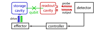
Figure 1: (Color online) Schematic setup of a circuit QED system used for constructing an arbitrary quantum channel.

The goal of this investigation is to expand the quantum control toolbox to efficiently implement all CPTP maps. In contrast to investigations of analog/digital quantum simulators of certain complex quantum dynamics Jaksch et al. (1998); Greiner et al. (2002); Buluta and Nori (2009); Lloyd (1996); Barreiro et al. (2011); Weimer et al. (2010); Lanyon et al. (2011); Salathé et al. (2015); Barends et al. (2015), we focus on the efficient implementation of CPTP maps for various quantum control tasks, including state stabilization, information processing, quantum error correction, etc.

This paper is organized as follows. First, we review the basic notation of CPTP maps using the Kraus representation in Section II. We then provide an explicit protocol that can implement arbitary CPTP maps using an ancilla qubit with QND readout and adaptive control, and describe its implementation with cQED in Section III. In Section IV, we illustrate potential applications of such constructed CPTP maps. In Section V, we discuss further extensions and various imperfections. Finally, we conclude the paper in Section VI.

II Kraus Representation

Mathematically, we use the Kraus representation for CPTP maps,

$$\mathcal{T}(\rho)=\sum_{i=1}^{N}K_{i}\rho K_{i}^{\dagger},$$ (1)

which are trace-preserving as ensured by the conditionChoi (1975)

$$\sum_{i=1}^{N}K_{i}^{\dagger}K_{i}=\mathbb{I}.$$ (2)

The Kraus operators $K_{i}$ do not have to be unitary or Hermitian. They can even be non-square matrices, if the input and output Hilbert spaces have different dimensions. By padding with zeros, we can always make them square matrices that describe a dimension-preserving channel for a system with dimension $d$. The Kraus representation is not unique, because for any $N\times N$ unitary matrix $U$, the set of new Kraus operators $F_{i}=\sum_{j}U_{ij}K_{j}$ characterizes the same CPTP map.

To efficiently construct a CPTP map, it is convenient to work with the Kraus representation with the minimum number of Kraus operators, called the Kraus rank of the CPTP map. Since there are at most $d^{2}$ linearly independent operators for a Hilbert space of dimension $d$, the Kraus rank is no larger than $d^{2}$ (for a rigorous treatment see Choi (1975)). There are efficient procedures to convert different representations of a channel to the minimal Kraus representation Choi (1975); Watrous (2011); Wilde (2016). For example, we may convert the Kraus representation into the Choi matrix (a $d^{2}\times d^{2}$ Hermitian matrix) and from there obtain the minimal Kraus representation Choi (1975). The second approach is to calculate the overlap matrix $C_{ij}=\mathrm{Tr}(K_{i}K_{j}^{\dagger})$ and then diagonalize it, $C=V^{\dagger}DV$ Nielsen and Chuang (2011). The new Kraus operators, $\tilde{K}_{i}=\sum_{j}V_{ij}K_{j}$, will be the most economic representation with some of them being zero matrices if the original representation is redundant. For cases with the CPTP map provided in other representations (e.g., super-operator matrix representation, Jamiolkowski/Choi matrix representation), we can also perform a well-defined routine to bring them into the minimal Kraus representation (as detailed in Appendix A).

III Universal Construction of Quantum Channels

As first pointed out by Lloyd and Viola Lloyd and Viola (2001), repeated application of Kraus rank-2 channels in an adaptive fashion is in principle sufficient to construct arbitrary open-system dynamics. Andersson and Oi provided a scheme for a binary-tree construction to explicitly implement an arbitrary POVM Andersson and Oi (2008). We extend the binary-tree scheme to a more general protocol for arbitrary CPTP maps. The procedure to construct a CPTP map with Kraus rank $N$ is associated with a binary tree of depth $L=\left\lceil\log_{2}N\right\rceil$, as shown in Fig. 2. In the following, we first consider the simple case with $L=1$, corresponding to the CPTP maps with Kraus rank $N\leq 2$. Then, we provide an explicit construction for general CPTP maps. After that, we outline how to physically implement the circuits using cQED as a promising physical platform.

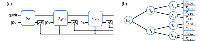
Figure 2: (Color online) (a) Quantum circuit for arbitrary channel construction. The dimension of the system $d$ can be arbitrary and the circuit depth depends only on the Kraus rank of the target channel. (b) Binary tree representation with depth $L=3$. The Kraus operators $K_{b^{\left(L\right)}}$ are associated with the leaves of the binary tree, $b^{\left(L\right)}\in\left\{0,1\right\}^{L}$. The system-ancilla joint unitary to apply in $l$-th round $U_{b^{\left(l\right)}}$ depends on the previous ancilla readout record $b^{\left(l\right)}=(b_{1}b_{2}\cdots b_{l})\in\left\{0,1\right\}^{l}$ associated with a node of the binary tree. For any given channel, all these unitaries can be explicited constructed and efficiently implemented.

III.1 Quantum Channels with Kraus Rank 2

Given a single use of the ancilla qubit, we can construct any rank-2 CPTP map, characterized by Kraus operators $\left\{K_{1},K_{2}\right\}$. The procedure consists of the following: (1) initialize the ancilla qubit in $\left|0\right>$, (2) perform a joint unitary operation $U\in SU(2d)$, and (3) discard (“trace over”) the ancilla qubit. Since this procedure has only one round of operation, there is no need for adaptive control and thus we can simply discard the ancilla without any measurement.

The $2d\times 2d$ matrix of unitary operation has the following block matrix form ,

$$U=\left(\begin{array}[]{cc}\left<0\right|U\left|0\right>&*\\ \left<1\right|U\left|0\right>&*\end{array}\right),$$ (3)

where the $d\times d$ submatrices are $\left<0\right|U\left|0\right>=K_{0}$, $\left<1\right|U\left|0\right>=K_{1}$, and “*” denotes irrelevant submatrices (as long as $U$ is unitary). The trace preserving requirement, $K_{0}^{\dagger}K_{0}+K_{1}^{\dagger}K_{1}=\mathbb{I}$, ensures that the condition $\sum_{b=0,1}\left(\left<b\right|U\left|0\right>\right)^{\dagger}\left<b\right|U\left|0\right>=\mathbb{I}_{d\times d}$ is fulfilled for unitary $U$. After discarding the ancilla qubit, the procedure achieves the CPTP map,

$$\mathcal{T}_{U}(\rho)=K_{0}\rho K_{0}^{\dagger}+K_{1}\rho K_{1}^{\dagger}.$$

Therefore, any channel with Kraus rank 2 can be simulated with a single use of the ancilla qubit .

If we measure the ancilla qubit instead of discarding it, we can in principle obtain the “which trajectory” information. More specifically, the system state becomes $\left(\left<0\right|U\left|0\right>\right)\rho\left(\left<0\right|U^{\dagger}\left|0\right>\right)$ (unnormalized) if we find the ancilla in $\left|0\right>$, and it becomes $\left(\left<1\right|U\left|0\right>\right)\rho\left(\left<0\right|U^{\dagger}\left|1\right>\right)$ if we find the ancilla in $\left|1\right>$. We may use the “which trajectory” information to determine later operations, and thus construct more complicated CPTP maps with higher Kraus rank.

III.2 Quantum Channels with Higher Kraus Rank

To implement a CPTP map with Kraus rank $N$, we need a quantum circuit with $L=\left\lceil\log_{2}N\right\rceil$ rounds of operations. Each round consists of (1) initialization of the ancilla qubit, (2) joint unitary gate over the system and ancilla (conditional on the measurement outcomes from previous rounds), (3) QND readout of the ancilla, and (4) storage of the classical measurement outcome for later use. For a quantum circuit consisting of $L$ rounds of operations with adaptive control (based on binary outcomes), there are $2^{L}-1$ possible intermediate unitary gates (associated with $2^{L}-1$ nodes of a depth-$L$ binary tree) and $2^{L}$ possible trajectories (associated with the $2^{L}$ leaves of the binary tree).

As illustrated in Fig. 2, we denote the $l$-th round unitary gate as $U_{b^{\left(l\right)}}$, associated with the node of the binary tree, $b^{\left(l\right)}=(b_{1}b_{2}\cdots b_{l})\in\left\{0,1\right\}^{l}$ with $l=0,\cdots,L-1$. (For $L=1$, there is only one unitary gate for $b^{\left(0\right)}=\varnothing$, which is $U_{b^{\left(0\right)}=\varnothing}$ as given in Eq. (3).) Generally, the unitary gate, $U_{b^{\left(l\right)}}$, has the following block matrix form

$$U_{b^{\left(l\right)}}=\left(\begin{array}[]{cc}\left<0\right|U_{b^{\left(l\right)}}\left|0\right>&*\\ \left<1\right|U_{b^{\left(l\right)}}\left|0\right>&*\end{array}\right),$$ (4)

where “*” again denote irrelevant submatrices (as long as $U_{b^{\left(l\right)}}$ is unitary). Since the ancilla always starts in $\left|0\right>$, it is sufficient to specify the $d\times d$ submatrices $\left<b_{l+1}\right|U_{b^{\left(l\right)}}\left|0\right>$ acting on the system, with the projectively measured ancilla state $\left|b_{l+1}\right>$ for $b_{l+1}=0,1$. Associated with the leaves of the binary tree, $b^{\left(L\right)}\in\left\{0,1\right\}^{L}$, are Kraus operators labeled in binary notation,

$$K_{b^{\left(L\right)}}=K_{i},$$ (5)

with $i=\left(b_{1}b_{2}\cdots b_{L}\right)_{2}+1$ and $K_{i>N}=0$. The singular value decomposition of each Kraus operator is $K_{b^{\left(L\right)}}=W_{b^{\left(L\right)}}D_{b^{\left(L\right)}}V_{b^{\left(L\right)}}^{\dagger}$.

We now provide an explicit construction for $\left<b_{l+1}\right|U_{b^{\left(l\right)}}\left|0\right>$. First, for each node $b^{\left(l\right)}$ with $l=1,\cdots,L-1$, we may diagonalize the non-negative Hermitian matrix (which is associated with the summation over all the leaves in the branch starting from $b^{\left(l\right)}$)

$$\sum_{b_{l+1},\cdots,b_{L}}K_{b^{\left(L\right)}}^{\dagger}K_{b^{\left(L\right)}}=V_{b^{\left(l\right)}}D_{b^{\left(l\right)}}^{2}V_{b^{\left(l\right)}}^{\dagger}\equiv M_{b^{\left(l\right)}}^{2},$$ (6)

with unitary matrix $V_{b^{\left(l\right)}}$, diagonal matrix $D_{b^{\left(l\right)}}$ consisting of non-negative diagonal elements, and Hermitian matrix $M_{b^{\left(l\right)}}=V_{b^{\left(l\right)}}D_{b^{\left(l\right)}}V_{b^{\left(l\right)}}^{\dagger}$. For notational convenience, we introduce $P_{b^{\left(l\right)}}$ as the support projection matrix of $D_{b^{\left(l\right)}}$, with elements

$$\left(P_{b^{\left(l\right)}}\right)_{j,k}=\mathrm{sign}\left[\left(D_{b^{\left(l\right)}}\right)_{j,k}\right],$$ (7)

where $\text{sign(0)}\equiv 0$, so that $P_{b^{\left(l\right)}}^{2}=P_{b^{\left(l\right)}}$ and $P_{b^{\left(l\right)}}D_{b^{\left(l\right)}}=D_{b^{\left(l\right)}}P_{b^{\left(l\right)}}=D_{b^{\left(l\right)}}$. The orthogonal projection is $P_{b^{\left(l\right)}}^{\perp}=\mathbb{I}-P_{b^{\left(l\right)}}$ and we also define the related projection $Q_{b^{\left(l\right)}}\equiv V_{b^{\left(l\right)}}P_{b^{\left(l\right)}}^{\perp}V_{b^{\left(l\right)}}^{\dagger}$. In addition, we define

$$\left(D_{b^{\left(l\right)}}^{-1}\right)_{j,k}=\begin{cases}1/\left(D_{b^{\left(l\right)}}\right)_{j,k}&\mbox{if $\left(D_{b^{\left(l\right)}}\right)\neq 0$}\\ 0&\mbox{otherwise.}\end{cases}$$ (8)

and denote the Moore-Penrose pseudo-inverse of $M_{b^{\left(l\right)}}$ as $M_{b^{\left(l\right)}}^{+}=V_{b^{\left(l\right)}}D_{b^{\left(l\right)}}^{-1}V_{b^{\left(l\right)}}^{\dagger}$. For $l=0$, we fix $V_{b^{\left(0\right)}}=D_{b^{\left(0\right)}}=D_{b^{\left(0\right)}}^{-1}=P_{b^{\left(0\right)}}=\mathbb{I}$ and $P_{b^{\left(0\right)}}^{\perp}=0$.

Finally, we have the explicit expression for the relevant submatrices of the unitary matrix

$$\left<b_{l+1}\right|U_{b^{\left(l\right)}}\left|0\right> =M_{b^{\left(l+1\right)}}M_{b^{\left(l\right)}}^{+}+\frac{1}{\sqrt{2}}Q_{b^{\left(l\right)}}$$ (9)

with $b^{\left(l+1\right)}=\left(b^{\left(l\right)},b_{l+1}\right)$ for $l=0,\cdots,L-2$, and

$$\left<b_{l+1}\right|U_{b^{\left(l\right)}}\left|0\right> =K_{b^{\left(l+1\right)}}M_{b^{\left(l\right)}}^{+}+\frac{1}{\sqrt{2}}W_{b^{\left(l+1\right)}}V_{b^{\left(l+1\right)}}^{\dagger}Q_{b^{\left(l\right)}}$$ (10)

for $l=L-1$. Since the isometric condition $\sum_{b_{l+1}=0,1}\left(\left<b_{l+1}\right|U_{b^{\left(l\right)}}\left|0\right>\right)^{\dagger}\left<b_{l+1}\right|U_{b^{\left(l\right)}}\left|0\right>=\mathbb{I}_{d\times d}$ is fulfilled (as proven in Appendix B), we can complete the unitary matrix $U_{b^{\left(l\right)}}$ with appropriate submatrices $\left<b_{l+1}\right|U_{b^{\left(l\right)}}\left|1\right>$.

For $L=1$, we use Eq. (10) for $l=0$ and obtain $\left<b_{1}\right|U_{b^{\left(0\right)}}\left|0\right>=K_{b^{\left(1\right)}}=\begin{cases}K_{1}&\mbox{for $b_{1}=0$}\\ K_{2}&\mbox{for $b_{1}=1$}\end{cases}$, which is consistent with the earlier construction for Kraus rank 2 channels.

With the above explicit construction of arbitrary CPTP maps, we will investigate the physical implementation with circuit QED.

III.3 Physical Implementation with Circuit QED

The above channel construction scheme relies on three key components: (1) ability to apply a certain class of unitary gates (recall that we engineer only the left half of the unitary) on the system and ancilla combined system; (2) QND readout of the ancilla qubit; (3) adaptive control of all unitary gates based on earlier rounds of QND measurement outcomes. Although there are a total of $(2^{n}-1)$ unitaries potentially to be applied, they can all be pre-calculated and one only needs to decide which one to perform in real time based on the measurement record. In principle any quantum system that meets these three requirements can be used to implement our scheme. In the following, we focus on a circuit QED system with a transmon qubit dispersively coupled to a microwave cavity with Hamiltonian Schuster et al. (2007)

$$\hat{H}_{0}=\omega_{c}\hat{a}^{\dagger}\hat{a}+\omega_{q}\left|e\right>\left<e\right|-\chi a^{\dagger}a\left|e\right>\left<e\right|,$$

where $\omega_{c}$ and $\omega_{q}$ are the cavity and qubit transition frequency respectively, $\hat{a}$ is the the annihilation operator of a cavity excitation, $\chi$ is the dispersive shift parameter and $\left|e\right>\left<e\right|$ is the qubit excited state projection. This is a promising platform to implement the channel construction scheme because the dispersive shift $\chi$ can be three orders of magnitude larger than the dissipation of the qubit and the cavity, allowing universal unitary control of the system Heeres et al. (2015); Krastanov et al. (2015).

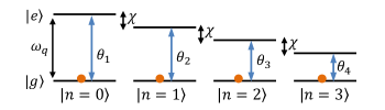
Figure 3: (Color online) Level diagram for the dispersively coupled qubit-cavity system. It is straightforward to implement $U_{\mathrm{ent}}$ for such a system by driving two level transitions that are spectrally separated. Here $g$/$e$ denote the ancilla qubit states ($0/1$ logical states) and $n$ denotes the photon number state.

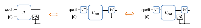
Figure 4: (Color online) For circuit QED systems, the $2d$-dimensional unitary used to generate an arbitrary Kraus rank-2 channel can be eventually simplified to unitaries acting on the system alone and an entangling operation $U_{ent}$ [Eq. (21)], which is a series of independent two-level transitions between $\left|g,\,n\right>$ and $\left|e,\,n\right>$, where $g$/$e$ denote the ancilla qubit states ($0/1$ logical states) and $n$ denotes the photon number state.

The Fock states of a cavity mode can be used to encode a $d$-dimensional system and the qubit can be used as the ancilla. Universal unitary control on the $d$-level system has been proposed in Ref. Krastanov et al. (2015) and demonstrated experimentally in Refs. Heeres et al. (2015, 2016). The strong dispersive coupling of the cavity and qubit enables selective driving of transitions between $\left|g,\,n\right>$ and $\left|e,\,n\right>$ for different excitation numbers $n$, which can implement the following entangling unitary gate

$$U_{\mathrm{ent}}(\theta_{i})$$ (13)

$$= \left(\begin{array}[]{c|c}S_{0}&-S_{1}\\ \hline\cr S_{1}&S_{0}\end{array}\right)$$

$$= \left(\begin{array}[]{ccc|ccc}\cos\frac{\theta_{1}}{2}&&&-\sin\frac{\theta_{1}}{2}\\ &\ddots&&&\ddots\\ &&\cos\frac{\theta_{d}}{2}&&&-\sin\frac{\theta_{d}}{2}\\ \hline\cr\sin\frac{\theta_{1}}{2}&&&\cos\frac{\theta_{1}}{2}\\ &\ddots&&&\ddots\\ &&\sin\frac{\theta_{d}}{2}&&&\cos\frac{\theta_{d}}{2}\end{array}\right)$$ (20)

$$= \prod_{n=0}^{d-1}\exp(-iY_{n}\theta_{n}/2),$$ (21)

where $Y_{n}\equiv-i\left|g,\,n\right>\left<e,\,n\right|+h.c.$ is the Pauli-$Y$ operator for the two-dimensional subspace associated with $n$ excitations (see Fig. 3). This entangling gate gives a channel described by Kraus operators $\{S_{0},\,S_{1}\}$. If we precede $U_{\mathrm{ent}}$ with a unitary $V^{\dagger}$ acting on the system alone and perform an adaptive unitary on the system after $U_{\mathrm{ent}}$ depending on the ancilla measurement $W_{0}$ or $W_{1}$, we end up with the unitary

$$U_{\mathrm{ent}}^{\prime} = \left(\begin{array}[]{cc}W_{0}&0\\ 0&W_{1}\end{array}\right)\left(\begin{array}[]{c|c}S_{0}&-S_{1}\\ \hline\cr S_{1}&S_{0}\end{array}\right)\left(\begin{array}[]{cc}V^{\dagger}&0\\ 0&V^{\dagger}\end{array}\right)$$

$$= \left(\begin{array}[]{cc}W_{0}S_{0}V^{\dagger}&*\\ W_{1}S_{1}V^{\dagger}&*\end{array}\right).$$

Remarkably, this construction is already sufficient to perfectly match the relevant two submatrices of the desired unitary

$$U=\left(\begin{array}[]{cc}\left<0\right|U\left|0\right>&*\\ \left<1\right|U\left|0\right>&*\end{array}\right),$$

with $\left<0\right|U\left|0\right>=W_{0}S_{0}V^{\dagger}$ and $\left<1\right|U\left|0\right>=W_{1}S_{1}V^{\dagger}$. To implement the quantum circuit in Fig. 2(a), we may explicitly identify the $W_{0/1}$, $S_{0/1}$, and $V$ matrices for unitary operations at different rounds $U=U_{b^{\left(l\right)}}$.

To justify the above claim, we provide an explicit design of $U_{\mathrm{ent}}^{\prime}$ to perfectly match the left two submatrices of $U_{b^{\left(l\right)}}$ in three steps. (1) We start with singular value decompositions (SVD) $\left<0\right|U\left|0\right>=W_{0}S_{0}V_{0}^{\dagger}$ and $\left<1\right|U\left|0\right>=W_{1}S_{1}V_{1}^{\dagger}$, where we have already set the $W$’s and $S$’s to their desired values. Now all that is left to do is to make sure that $V_{0}=V_{1}=V$. To uniquely determine the decomposition, we require that the singular values in $S_{0}$ are arranged in descending order $\left(S_{0}\right)_{j,j}\geq\left(S_{0}\right)_{j+1,j+1}$, while the singular values in $S_{1}$ are arranged in ascending order $\left(S_{1}\right)_{j,j}\leq\left(S_{1}\right)_{j+1,j+1}$. (2) The isometric condition $\sum_{b=0,1}\left(\left<b\right|U\left|0\right>\right)^{\dagger}\left<b\right|U\left|0\right>=\mathbb{I}_{d\times d}$ requires that $V_{0}^{\dagger}V_{1}S_{1}^{2}V_{1}^{\dagger}V_{0}=\mathbb{I}_{d\times d}-S_{0}^{2}.$ Since both $S_{1}^{2}$ and $\mathbb{I}_{d\times d}-S_{0}^{2}$ are diagonal with elements in ascending order, $V_{1}^{\dagger}V_{0}$ must be the identity – that is, $V_{0}=V_{1}=V$. Therefore, we have obtained all the components of $U^{\prime}_{\mathrm{ent}}$, which fulfills $\left<0\right|U\left|0\right>=W_{0}S_{0}V^{\dagger}$ and $\left<1\right|U\left|0\right>=W_{1}S_{1}V^{\dagger}$. A similar property was used in Dressel et al. (2014) to simplify the contruction of generalized measurements of a qubit. In terms of circuits, we decomposed the $2d$-dimensional unitaries in Fig. 2 into a series of simpler operations, as shown in Fig. 4.

IV Application Examples

The concept of CPTP maps encompasses all physical operations ranging from cooling, quantum gates, measurements, to dissipative dynamics. The capability to construct an arbitrary CPTP map offers a unified approach to all aspects of quantum technology. To illustrate the wide range of impact of quantum channel construction, we now investigate some interesting applications, including quantum system initialization/stabilization, quantum error correction, Lindbladian quantum dynamics, exotic quantum channels, and quantum instruments.

IV.1 Initialization/Stabilization

Almost all quantum information processing tasks require working with a well-defined (often pure) initial state. One common approach is to sympathetically cool the system to the ground state by coupling to a cold bath, or optically pumping to a specific dark state, and then performing unitary operations to bring the system to a desired initial state. This can be slow if the system has a large relaxation time scale. Another approach is to actively cool the system by measurement and adaptive control. Along the line of the second approach, the channel construction technique can be applied to discretely pump the system from an arbitrary state into the target state $\sigma$, which can be pure or mixed. The pumping time depends on the quantum gate and measurement speed, instead of the natural relaxation rate.

It is well known that the CPTP map

$$\rho\mapsto\mathcal{E}_{\mathrm{Init}}\left(\rho\right)=\mathrm{Tr}(\rho)\sigma$$

stabilizes an arbitrary state $\sigma$ Watrous (2011); Wilde (2016). If the target state has diagonal representation $\sigma=\sum_{\mu}\lambda_{\mu}\left|\psi_{\mu}\right>\left<\psi_{\mu}\right|$, where $\lambda_{\mu}\geq 0$ and $\sum_{\mu}\lambda_{\mu}=1$, one explicit form of Kraus operators is $\left\{K_{i}^{\mu}=\sqrt{\lambda_{\mu}}\left|\psi_{\mu}\right>\left<i\right|\right\}$, where $\left|i\right>$ are a basis of the system Hilbert space Wu et al. (2007). Contrary to the conventional approaches discussed in the previous paragraph, this dissipative map bundles the cooling and state preparation steps and pumps an arbitrary state into state $\sigma$. Depending on $\sigma$, entropy can be extracted from or injected into the system by the ancilla qubit. If we run the channel construction circuit repeatedly, state stabilization can be achieved.

Besides pure state initialization for quantum information processing, preparation of carefully designed mixed states may find application in the study of foundational issues of quantum mechanics such as quantum discord, quantum contextuality, and quantum thermodynamics Ollivier and Zurek (2001); Henderson and Vedral (2001); Kirchmair et al. (2009); Zu et al. (2012); Oppenheim (2013); Brandao et al. (2015).

IV.2 Quantum Error Correction

Besides unique steady states, there are CPTP maps that can stabilize multiple steady states or even a subspace of steady states, which may be used to encode useful classical or quantum information. A practically useful application of such CPTP maps with subspaces of steady states is quantum error correction (QEC). Typical QEC schemes encode quantum information in some carefully chosen logical subspaces Gottesman (1997); Nielsen and Chuang (2011) (or subsystems Bacon (2006)), and use syndrome measurement and conditional recovery operations to actively decouple the system from the environment. Despite the variety of QEC codes and recovery schemes, the operation of any QEC recovery can always be identified as a quantum channel.

For qubit-based stabilizer codes with $N_{s}$ stabilizer generators, the recovery is a CPTP map with Kraus rank $2^{N_{s}}$ Nielsen and Chuang (2011). We may first use the ancilla to sequentially measure all $N_{s}$ stabilizer generators to extract the syndrome, and finally perform a correction unitary operation conditioned on the syndrome pattern. Since the stabilizer generators commute with each other, their ordering does not change the syndrome. Moreover, the stabilizer measurement does not require conditioning on previous measurement outcomes, because the unitary operation at the $l$-th round is simply $U_{b^{\left(l\right)}}=U_{l}=P_{+}\otimes\hat{S}_{l}+P_{-}\otimes I$ with $\hat{S}_{l}$ for the $l$-th stabilizer and $P_{\pm}=\frac{1}{2}\left(\left|g\right>\pm\left|e\right>\right)\left(\left<g\right|+\left<e\right|\right)$, which is independent of the previous measurement outcomes $b^{\left(l-1\right)}$. Finally, we perform the correction unitary operation $U_{b^{\left(N_{s}\right)}}$ conditioned on the syndrome $b^{\left(N_{s}\right)}$.

Generally, we may consider all QEC codes that fulfill the quantum error-correction conditions associated with a set of error operations Knill and Laflamme (1997); Nielsen and Chuang (2011). For these QEC codes, we can explicitly obtain the Kraus representation of the QEC recovery map Knill and Laflamme (1997); Nielsen and Chuang (2011), which can be efficiently implemented with our construction of quantum channels. For example, let us consider the binomial code Michael et al. (2016), which uses the larger Hilbert space of higher excitations to correct excitation loss errors in bosonic systems. In order to correct up to two excitation losses, the binomial code encodes the two logical basis states as

$$\left|W_{\uparrow}\right> \equiv \frac{\left|0\right>+\sqrt{3}\left|6\right>}{2},$$

$$\left|W_{\downarrow}\right> \equiv \frac{\sqrt{3}\left|3\right>+\left|9\right>}{2}.$$

For small loss probability $\gamma$ for each excitation, this encoding scheme can correct errors up to $O\left(\gamma^{2}\right)$, which includes the following four relevant processes: identity evolution ($\hat{I}$), losing one excitation ($\hat{a}$), losing two excitations ($\hat{a}^{2}$), and back-action induced dephasing ($\hat{n}$) Michael et al. (2016). Based on the Kraus representation of the QEC recovery (with Kraus rank 4), we can obtain the following set of unitary operations $U_{b^{\left(l\right)}}$ for the construction of the QEC recovery channel with an adaptive quantum circuit:

$$\tilde{U}_{\varnothing} = \left(\begin{array}[]{c}\hat{P}_{3}\\ \hat{I}-\hat{P}_{3}\end{array}\right),$$

$$\tilde{U}_{0} = \left(\begin{array}[]{c}\hat{P}_{W}\\ \hat{I}-\hat{P}_{W}\end{array}\right),\ \tilde{U}_{1}=\left(\begin{array}[]{c}\hat{P}_{1}\\ \hat{I}-\hat{P}_{1}\end{array}\right),$$

$$\tilde{U}_{00} = \left(\begin{array}[]{c}\hat{I}\\ \hat{0}\end{array}\right),\ \tilde{U}_{01}=\left(\begin{array}[]{c}U_{\hat{n}}\\ \hat{0}\end{array}\right),$$

$$\tilde{U}_{10} = \left(\begin{array}[]{c}U_{\hat{a}}\\ \hat{0}\end{array}\right),\ \tilde{U}_{11}=\left(\begin{array}[]{c}U_{\hat{a}^{2}}\\ \hat{0}\end{array}\right),$$

where the projections are defined as $\hat{P}_{i}\equiv\sum_{k}\left|3k+i\right>\left<3k+i\right|$ and $\hat{P}_{W}\equiv\left|W_{\uparrow}\right>\left<W_{\uparrow}\right|+\left|W_{\downarrow}\right>\left<W_{\downarrow}\right|$, and the unitary operators $U_{\hat{O}}$ ($\hat{O}=\hat{a},\,\hat{a}^{2},\,\hat{n}$) transform the error states $\hat{O}\left|W_{\sigma}\right>$ back to $\left|W_{\sigma}\right>$ for $\sigma=\uparrow,\,\downarrow$. Explicitly,

$$U_{\hat{O}}=\sum_{\sigma}\left|W_{\sigma}\right>\frac{\left<W_{\sigma}\right|\hat{O}^{\dagger}}{\sqrt{\left<W_{\sigma}\right|\hat{O}^{\dagger}\hat{O}\left|W_{\sigma}\right>}}+U^{\perp},$$

where $U^{\perp}$ is any isometry that takes the complement of the syndrome subspace to the complement of the logical subspace. In the first two rounds, we perform the projective measurements to extract the error syndrome. In the last round, we apply a correction unitary operation to restore the logical states. Specifically, if the measurement outcome $b^{\left(2\right)}=(0,0)$, there is no error and identify operation $\hat{I}$ is sufficient. If $b^{\left(2\right)}=(0,1)$, there is back-action induced dephasing error, which changes the coefficients of Fock states so we need to correct for that with $U_{\hat{n}}$. If $b^{\left(2\right)}=(1,1)$, there is a single excitation loss, which can be fully corrected with $U_{\hat{a}}$. If $b^{\text{$\left(2\right)$}}=\left(1,0\right)$, there are two excitation losses, which can be fully corrected with $U_{\hat{a}^{2}}$. Repetitive application of the above QEC recovery channel can stabilize the system in the code space spanned by $\left|W_{\uparrow}\right>$ and $\left|W_{\downarrow}\right>$.

More interestingly, beyond exact QEC codes there are approximate QEC codes Leung et al. (1997); Ng and Mandayam (2010a); Bény and Oreshkov (2010); Mandayam and Ng (2012), which can also efficiently correct errors but only approximately fulfill the QEC criterion. For approximate QEC codes, it is very challenging to analytically obtain the optimal QEC recovery map, but one can use semi-definite programming to numerically optimize the entanglement fidelity and obtain the optimal QEC recovery map Fletcher et al. (2007); Fletcher (2007); Albert et al. ; Audenaert and De Moor (2002). Alternatively one can use the transpose channel Ng and Mandayam (2010b) or quadratic recovery channels Bény and Oreshkov (2010, 2011); Tyson (2010) which are known to be near-optimal. All these recovery channels can be efficiently implemented with our general construction of CPTP maps.

IV.3 Markovian Channels

Recently, there has been growing interest in designing and engineering open system dynamics for quantum information processing Sweke et al. (2015); Bacon et al. (2001); Verstraete et al. (2009); Diehl et al. (2011); Paulisch et al. (2016), which uses Markovian channels

$$\rho\rightarrow\mathcal{E}_{\mathrm{MC},t}\left(\rho\right)=\mathbb{T}\left[e^{\int_{0}^{\tau}\mathcal{L}_{t}dt}\right]\rho,$$

where $\mathbb{T}$ stands for time ordering, and $\mathcal{L}_{t}$ is the time-dependent Lindbladian operator that has general form

$$\mathcal{L}_{t}(\rho) = -\frac{i}{\hbar}\left[H,\,\rho\right]$$

$$+\sum_{n,m}h_{n,m}\left[L_{n}\rho L_{m}^{\dagger}-\frac{1}{2}(\rho L_{m}^{\dagger}L_{n}+L_{m}^{\dagger}L_{n}\rho)\right],$$

where $L_{n}$ are jump operators. Markovian channels are a special class of CPTP maps Wolf and Cirac (2008). In contrast to the continuous time evolution approach Bacon et al. (2001); Sweke et al. (2015); Zanardi et al. (2016), we construct $\mathcal{E}_{\mathrm{MC},t}=\mathcal{T}\left[e^{\int_{0}^{\tau}\mathcal{L}_{t}dt}\right]$ directly, which is advantageous in that it does not take more time to see results for larger $\tau$ because no Trotterization or stroboscopic control is required. We consider the following cat-pumping example to manifest these points.

Using a specifically engineered dissipation for a cavity mode, one can stabilize a two-dimensional steady-state subspace spanned by the so called cat-code Mirrahimi et al. (2014); Leghtas et al. (2015). The required dissipation can be described by the following time-independent Lindbladian,

$$\mathcal{L}(\rho)=J\rho J^{\dagger}-\frac{1}{2}(J^{\dagger}J\rho+\rho J^{\dagger}J),$$

where the jump operator $J$ is

$$J=\sqrt{\kappa}\prod_{i}^{n}(a-\alpha_{i}).$$

The complex variables $\alpha_{i}$ determine the coherent state components $\left|\alpha_{i}\right>$ that span the steady-state subspace. As proposed in Mirrahimi et al. (2014) and demonstrated in Leghtas et al. (2015), the dissipation can be engineered by coupling the system mode and another lossy mode with Hamiltonian $H=J^{\dagger}b+h.c.$ where $b$ is the annihilation operator for the lossy mode. Practically, it is challenging to generate desired engineered dissipation that is much stronger than the undesired dissipations (e.g., dephasing, Kerr effect, etc). In addition, it is difficult to extract the Hamiltonian $H$ associated with higher-order nonlinearity, in order to have a higher-dimensional steady state subspace with more coherent components. With our approach, however, the effective rate $\kappa$ can be large and determined by the time scale to implement the circuits, which is limited by the duration of gates and measurements, and the delay of adaptive control. Moreover, the construction can easily extend to the case that simultaneously stabilizes many coherent components.

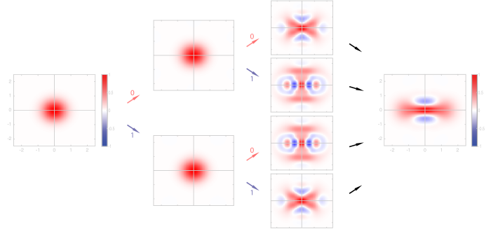
Figure 5: (Color online) All possible trajectories for pumping a vacuum state $\left|0\right>$ to the subspace spanned by $\left|\pm\alpha\right>$ with $\alpha=1.1$. Depending on the probabilistic ancilla readout, the system evolves along different trajectories in each run of the circuit. However, since the steady state of the system is a pure state $\left|\psi_{\mathrm{f}}\right>=\left(\left|\alpha\right>+\left|-\alpha\right>\right)/\sqrt{2}$, which cannot be decomposed as a probabilistic mixture of different states, the final state for each trajectory is always the same pure state $\left|\psi_{\mathrm{f}}\right>$. The two outcomes of the first round are only slightly different. Two of the four outcomes of the second round are also very similar to the others.

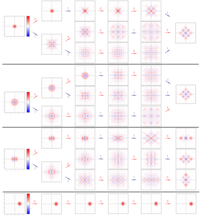
Figure 6: (Color online) Example trajectories for 4-component cat pumping starting with four different initial states, $\left|0\right>,$ $\left|2\right>$, $\left(\left|0\right>+\left|2\right>\right)/\sqrt{2}$ and coherent state $\left|\tilde{\alpha}=2.3\right>$. Here the steady coherent components are $\left|\alpha\right>$, $\left|i\alpha\right>$, $\left|-\alpha\right>$, and $\left|-i\alpha\right>$ with $\alpha=2.5$. The binary number on the arrow indicates the ancilla measurement outcome. For the first two cases, since the steady state is a pure state which cannot be decomposed as a probabilistic mixture of different states, the final state for each trajectory is always the same pure state $\left|\psi_{\mathrm{f}}\right>$. For the third case, the steady state is a mixed state $\rho_{\mathrm{f}}$, so different trajectories give different pure states. Since the ancilla measurement results are discarded, the output state for the system is an ensemble of the different final states, which coincides with $\rho_{\mathrm{f}}$. The fourth case starts near the steady state subspace and is slowly pulled into it. The trajectory shown is the dominant one which is taken with probability higher than 0.96. Dashed circles show the position of $\left|\alpha=2.5\right>$.

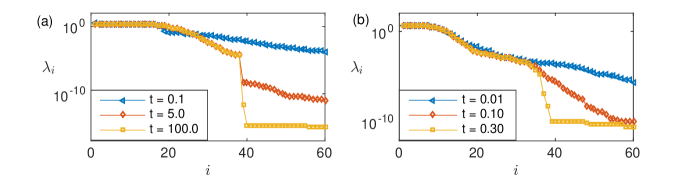
Figure 7: (Color online) The magnitudes of the Kraus operators $\lambda_{i}\equiv\mathrm{Tr}(K_{i}^{\dagger}K_{i})$, corresponding to $\mathcal{E}_{t}=\exp(\mathcal{L}\,t)$ for (a) two-legged cat pumping and (b) four-legged cat pumping. Here we set $\kappa=1$. In the long time limit, both channels have Kraus rank approximately equal to the size of the truncated Hilbert space $d=n_{c}+1$ where $n_{c}$ is the maximal photon number. We treat all $\lambda_{i}$ smaller than $10^{-10}$ as 0. The figures show results with $n_{c}=38$ but we verified that our observation remains valid for any sufficiently large $n_{c}$.

With the channel construction presented here, we can now obtain Lindbladian dynamics $\mathcal{E}_{\mathrm{MC},t}=\exp(\mathcal{L}\,t)$ for any given $t$. Sometimes we are interested in the channel for $t\rightarrow\infty$ (or equivalently the strong pumping limit $\kappa\rightarrow\infty$), $\mathcal{E}_{\mathrm{MC},\infty}$, and it was recently shown that any more general (i.e., non-Markovian) channel can be embedded in $\mathcal{E}_{\mathrm{MC},\infty}$ Albert et al. (2016b). For our approach, sending $t$ to $\infty$ does not cost us an infinite amount of time, since the number of cycles in our construction circuit only scales logarithmically with the Kraus rank of $\mathcal{E}_{MC,\infty}$. In numerical calculations, the Kraus rank is not a clear-cut quantity even when we have obtained the most economic Kraus representation. So we define and examine the “magnitudes” of the Kraus operators, $\lambda_{i}\equiv\mathrm{Tr}(K_{i}^{\dagger}K_{i})$ and remove $K_{i}$ from the description of the channel if $\lambda_{i}<10^{-10}$. Note that $\lambda_{i}/d$ is the probability for $K_{i}$ to act on the system when the input state is the maximally mixed state, $\rho=I/d$. The $\lambda_{i}$ also turn out to be the eigenvalues of the Choi matrix, see Appendix A for details. Numerically we found that $\mathcal{E}_{\infty}$ has lower Kraus rank than $\mathcal{E}_{MC,t}$ with finite $t$, see Fig. 7 for two examples. In the infinite time limit, the Kraus rank scales linearly with the dimension of the truncated Hilbert space $d=n_{c}+1$ (whre $n_{c}$ is the photon number truncation), much smaller than the largest possible value $d^{2}$.

Figure 5 and figure 6 (corresponding to $n=2$ and $n=4$ coherent components) show trajectories of the system evolution under our constructed channel for a large $t\sim 10^{3}/\kappa$. In each run of the simulation, the ancilla measurement results that correspond to different trajectories are probabilistic. If the system starts in $\left|0\right>$, $\left|1\right>$, or $\left|2\right>$, the correct steady state is pure. So whichever trajectory the system follows, it ends up in the same pure state. If the system starts in a state like $\left(\left|0\right>+\left|2\right>\right)/\sqrt{2}$, the steady state is a mixed state, in which case different trajectories lead to different final states. But the probabilistic mixture of all these final states make up the expected steady state density matrix $\rho_{\mathrm{f}}=\mathcal{E}_{t}(\rho_{\mathrm{init}})$.

Our approach of constructing CPTP maps thus provides another promising pathway to efficiently pump the cavity mode into the cat-code subspace using approximately $\log_{2}(d)$ rounds of operations, each of which consists of adaptive $SU\left(2d\right)$ unitary gates, qubit QND measurement, and storing the measurement outcome. In the exact same fashion, we can construct CPTP maps that manipulate the logical states living in the code subspace, which can, e.g., implement a digital version of holonomic gates Albert et al. (2016c).

IV.4 Exotic Channels

Besides Markovian channels, there are also exotic CPTP maps that cannot be obtained from time dependent Lindbladian master equations. Hence, these channels are not accessible in previous proposals of open system evolution under Lindbladian master equations Bacon et al. (2001); Sweke et al. (2015); Zanardi et al. (2016). For example, we can define the following CPTP map (called the “partial corner transpose” channel) for $d$-dimensional systems Wolf and Cirac (2008)

$$\mathcal{T}(\rho)=\frac{\rho^{T_{c}}+\mathbb{I}\,\mathrm{Tr}(\rho)}{1+d},$$

where $\rho^{T_{c}}$ is the “corner transposed” density matrix (i.e. exchanging the matrix elements $\rho_{1,d}$ and $\rho_{d,1}$ while keeping all other elements unchanged). Following Ref. Wolf and Cirac (2008), the partial corner transpose channel has diagonal representation in the generalized Gell-Mann basis, with identical eigenvalues $1/\left(d+1\right)$, except for two basis elements – the eigenvalue is $1$ for basis element $I_{d\times d}/\sqrt{d}$, and the eigenvalue is $-1/\left(d+1\right)$ for basis element $\left(\left|d\right>\left<1\right|+\left|1\right>\left<d\right|\right)/\sqrt{2}$. Hence, the determinant $\mathrm{det}\mathcal{T}=-\left(d+1\right)^{1-d^{2}}$ is negative. In contrast, the determinant for Markovian channels are always non-negative. Therefore, the partial corner transpose cannot be obtained from Markovian channels.

We have obtained an explicit construction of $\left\{U_{b^{\left(l\right)}}\right\}$ for the partial corner transpose channel with $d=3$, as detailed in Appendix C. For our channel construction approach, the unitaries $U_{b^{\left(l\right)}}$ seem to be no more difficult from other more conventional channels with the same rank.

IV.5 Quantum Instrument and POVM

The construction of CPTP maps can be further extended if the intermediate measurement outcomes are part of the output together with the state of the quantum system, which leads to an interesting class of quantum channel called a quantum instrument (QI) Wilde (2016); Watrous (2011); Blumoff et al. (2016). QIs enable us to track both the classical measurement outcome and the post-measurement state of the quantum system. Mathematically, the quantum instrument has the following CPTP map:

$$\rho\mapsto\mathcal{E}_{\mathrm{QI}}\left(\rho\right)=\sum_{\mu=1}^{M}\mathcal{E}_{\mu}(\rho)\otimes\left|\mu\right>\left<\mu\right|,$$ (28)

where $\left|\mu\right>\left<\mu\right|$ are orthogonal projections of the measurement device with $M$ classical outcomes, and $\mathcal{E}_{\mu}$ are completely positive trace non-increasing maps, while $\sum_{\mu=1}^{M}\mathcal{E}_{\mu}(\rho)$ preserves the trace. Note that $\mathcal{E}_{\mu}(\rho)$ gives the post-measurement state associated with outcome $\mu$.

As illustrated in Fig. 8, our channel construction can implement the QI as follows. (1) Find the minimum Kraus representation for $\mathcal{E}_{\mu}$ (each with rank $J_{\mu}$) with Kraus operators $K_{\mu,j}$ for $j=1,\,2,\,\cdots,\,J_{\mu}$. (2) Introduce binary labeling of these Kraus operators, $K_{\vec{b}^{(L)}}$, where the binary label has length $L=L_{1}+L_{2}$ with the first $L_{1}=\left\lceil\log_{2}M\right\rceil$ bits $b^{(L_{1})}$ to encode $\mu$ and the remaining $L_{2}=\left\lceil\log_{2}\max_{\mu}(J^{\mu})\right\rceil$ bits to encode $j$ (padding with zero operators to make a total of $2^{L}$ Kraus operators). (3) Use the quantum circuit with $L$ rounds of adaptive evolution and ancilla measurement. (4) Output the final state of the quantum system as well as $b^{(L_{1})}$ that encodes $\mu$ associated with the $M$ possible classical outcomes. This enables us to construct the arbitrary QI described in Eq. (28). The QI is a very useful tool for implementation of complicated conditional evolution of the system. It can be used for quantum information processing tasks that require measurement and adaptive control.

If we remove the quantum system from the QI output, we effectively implement a positive operator valued measure (POVM), which is also referred to as a generalized quantum measurement. A POVM is a CPTP map from the quantum state of the system to the classical state of the measurement device

$$\rho\mapsto\mathcal{E}_{\mathrm{POVM}}\left(\rho\right)=\sum_{\mu=1}^{M}\mathrm{Tr}\left[\Pi_{\mu}\rho\right]\left|\mu\right>\left<\mu\right|,$$

which is characterized by a set of Hermitian positive semidefinite operators $\{\Pi_{\mu}\}_{\mu=1}^{M}$ that sum to the identify operator $\sum_{\mu}\Pi_{\mu}=\mathbb{I}$. For positive semidefinite $\Pi_{\mu}$, we can decompose it as $\Pi_{\mu}=\sum_{j}K_{\mu,j}^{\dagger}K_{\mu,j}$ with a set of Kraus operators $\left\{K_{\mu,j}\right\}_{j=1,\cdots,J_{\mu}}$. Therefore, the circuit for the quantum instrument also implements the POVM if we remove the quantum system from the QI output, $\mathcal{E}_{\mathrm{POVM}}\left(\rho\right)=\mathrm{Tr_{sys}}\left[\mathcal{E}_{\mathrm{QI}}\left(\rho\right)\right]$, which reduces to the binary tree construction scheme of a POVM as proposed by Andersson and Oi Andersson and Oi (2008). A POVM can be useful for quantum state discrimination. It is known to be impossible for any detector to perfectly discriminate a set of non-orthogonal quantum states. An optimal detector can achieve the so-called Hellstrom bound Helstrom (1976), by properly designing a POVM (in this case a PVM–projection valued measure). For example, in optical communication, quadrature phase shift keying uses four coherent states with different phases $\left|\alpha\right>$, $\left|i\alpha\right>$, $\left|-\alpha\right>$ and $\left|-i\alpha\right>$ to send two classical bits of information. With our scheme it is straightforward to implement the optimal POVM given in Ref. Osaki et al. (1996), which is a rank-4 POVM.

As summarized in Fig. 8, we may classify three different situations for CPTP maps based on the output: (a) standard quantum channel with the quantum system as the output, (b) POVM with the classical measurement outcomes as the output, (c) QI with both the quantum system and the classical measurement outcomes for the output. In principle, all three situations can be reduced to the standard quantum channel with an expanded quantum system that includes an additional measurement device to keep track of the classical measurement outcomes. In practice, however, it is much more resource efficient to use a classical memory for classical measurement outcomes, so that we can avoid working with the expanded quantum system.

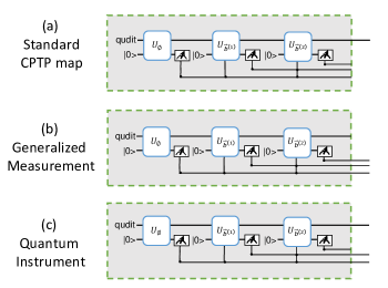
Figure 8: (Color online) Three different types of CPTP maps. (a) To implement a standard CPTP on the system qudit, all ancilla measurement records should be thrown away; (b) A generalized measurement does not concern the system state after measurement, so only the ancilla measurement record is kept; (c) A quantum instrument keeps the both the post-measurement state of the system and outcome $\mu$, encoded by the first $L_{1}$ bits of the ancilla measurement record. The remaining $L_{2}$ bits of the measurement record are thrown away. In the figure, $L_{1}=2$ and $L_{2}=1$.

V Discussion

So far, we have assumed a two-level ancilla for our channel construction, which can be generalized to an ancilla with higher dimensions. If we use an $s$-dimensional ancilla, we can use an s-ary tree construction of the quantum channel with Kraus rank $N$, consisting of $\left\lceil\log_{s}N\right\rceil$ rounds of adaptive evolution and ancilla measurement.

We emphasize that the adaptive control is essential for arbitrary channel construction with a small (low-dimensional) ancilla. Without adaptive control, the constructed channel is a product of channels, $\mathcal{T}=\cdots\mathcal{T}_{3}\mathcal{T}_{2}\mathcal{T}_{1}$, and it excludes indivisible channels which cannot be constructed with a single round of operation or decomposed into a product of non-unitary channels Wolf and Cirac (2008). Although the approach of Trotterization and stroboscopic control can construct Markovian channels without adaptive control, that approach has an overhead that increases with the duration of the Markovian evolution Zanardi et al. (2016), while our construction has a bounded overhead that scales logarithmically with the relevant dimensions of the quantum system.

Besides developing a control toolbox for quantum information processing, our channel construction protocol may also be useful for investigating open quantum systems, with the potential advantages of reduced overhead in channel construction and the new ingredient of indivisible channels, which are not accessible with conventional reservoir engineering of Markovian channels Diehl et al. (2008); Weimer et al. (2010); Bardyn et al. (2013); Morigi et al. (2015); Budich et al. (2015).

In experimental realizations, there will be imperfections in the unitary gates $U_{b^{\left(l\right)}}$ and ancilla measurements. Fortunately, the quantum circuit for channel construction only has $n=\left\lceil\log_{2}\mbox{N}\right\rceil\leq\left\lceil 2\log_{2}d\right\rceil$ rounds of gate and measurement. If the error per round is $\epsilon$, then the overall error rate of the channel construction is only $n\epsilon\sim\epsilon\log_{2}d$. More rigorously, we may use the diamond norm distance $\epsilon_{\diamond}$ to upper bound the error associated with each round of operation Wilde (2016), and $n\epsilon_{\diamond}$ rigorously bounds the diamond norm distance of the constructed quantum channel.

VI Conclusion

We have provided an explicit procedure to construct arbitrary CPTP maps, assisted by an ancilla qubit with QND readout and adaptive control. Our construction has various applications, including system initialization/stabilization, quantum error correction, Markovian and exotic channel simulation, and generalized quantum measurement/quantum instruments construction. Such a construction can be implemented with circuit QED and various other physical platforms.

Appendix A Representations of Quantum Channels

In this appendix we review some basics on alternative ways a CPTP map can be represented and how to convert back and forth between different representations. Since our scheme favors the Kraus representation as our “canonical representation”, it is important to understand how to convert a target channel in other representations to the Kraus form.

A.1 Superoperator Matrix Representation

Since CPTP maps are linear in the density matrix $\rho$, we can treat $\rho$ as a vector and write down the matrix form of the super-operator $\mathcal{T}$, such that

$$\tilde{\rho}_{ij}=\sum_{m,n}T_{ij,mn}\rho_{mn}$$

or

$$\vec{\tilde{\rho}}=T\cdot\vec{\rho}$$

where $\tilde{\rho}=\mathcal{T}(\rho)$. This matrix form is particularly useful when one considers the concatenation of channels. Applying channel $\mathcal{T}_{1}$ first and then $\mathcal{T}_{2}$ results in the overall channel represented by the matrix $T=T_{2}\cdot T_{1}$, where “$\cdot$” indicates matrix multiplication. The matrix form also allows one to characterize channels with the determinant, $\det(T)$. One interesting property is that for Markovian channels or Kraus rank-2 channels, the determinant is always positive Wolf and Cirac (2008). The downside of this representation is that it is not obvious whether a given $T$ qualifies as a CPTP map. We will need to convert it to the Jamiolkowski/Choi matrix representation or Kraus representation to verify that. Conversely, given a channel in Kraus form, the super-operator matrix can be obtained straightforwardly,

$$T=\sum_{i}^{N}K_{i}\otimes K_{i}^{*}.$$

A.2 Jamiolkowski/Choi Matrix Representation

From the well known channel-state duality (Jamiolkowski-Choi isomorphism) Jamiolkowski (1972); Choi (1975) we know that each channel $\mathcal{T}$ for a system with d-dimensional Hilbert space $\mathcal{H}$ corresponds (one-to-one) to a state (a density matrix) on $\mathcal{H}\otimes\mathcal{H}$,

$$\tau=(\mathcal{T}\otimes\mathcal{I})(\left|\Omega\right>\left<\Omega\right|)$$

where $\left|\Omega\right>=\frac{1}{\sqrt{d}}\sum_{i}\left|i\right>\otimes\left|i\right>$ is the maximally entangled state of the two subsystems. A closely related matrix is the Choi matrix which is only a constant multiple of the Jamiolkowski matrix, $M=d\,\tau$, where $d$ is the dimension of the Hilbert space. A convenient fact to note is that $M$ and the super-operator matrix $T$ are related in a simple way,

$$T_{ij,mn}=M_{im,jn}.$$

Being a density matrix, $\tau$ is Hermitian. Moreover $\tau$ is semi-positive definite if and only if $\mathcal{T}$ is completely positive; $\tau$ is normalized if $\mathcal{T}$ is trace preserving.

It is straightforward to convert the Choi matrix $M$ to the Kraus representation. If $M$ is diagonalized,

$$M=\sum_{i}\lambda_{i}v_{i}v_{i}^{\dagger},$$

where $v_{i}$ are $d^{2}$ dimensional eigenvectors of $\tau$, the Kraus operators are obtained by rearranging $\sqrt{\lambda_{i}}v_{i}$ as $d\times d$ matrices. Clearly the number of non-zero eigenvalues $\lambda_{i}$ is the Kraus rank of the corresponding channel. Later we will often check the eigenvalue spectrum of the Choi matrix of a channel to determine its Kraus rank. For numerical calculation we usually make a truncation of the eigenvalues. For example, we may set all eigenvalues smaller than $10^{-10}$ to 0.

Appendix B Proof of Quantum Channel Construction

We now prove that our channel construction correctly implements the target CPTP map. To justify the channel construction, we need to show that (a) the submatrices $\left<b_{l+1}\right|U_{b^{\left(l\right)}}\left|0\right>$ fulfill the isometry condition

$$\sum_{b_{l+1}=0,1}\left(\left<b_{l+1}\right|U_{b^{\left(l\right)}}\left|0\right>\right)^{\dagger}\left<b_{l+1}\right|U_{b^{\left(l\right)}}\left|0\right>=\mathbb{I}_{d\times d}$$ (29)

for all $b^{\left(l\right)}$ and $l=1,2,\cdots,L-1$, and (b) the accumulated evolution along the binary tree indeed implements the corresponding Kraus operator

$$\left(\left<b_{L}\right|U_{b^{\left(L-1\right)}}\left|0\right>\right)\cdots\left(\left<b_{l+1}\right|U_{b^{\left(l\right)}}\left|0\right>\right)\cdots\left(\left<b_{1}\right|U_{b^{\left(0\right)}}\left|0\right>\right)=K_{b^{\left(L\right)}}.$$ (30)

First, we show that

$$V_{b^{\left(l\right)}}D_{b^{\left(l\right)}}^{2}V_{b^{\left(l\right)}}^{\dagger}=\sum_{b_{l+1},\cdots,b_{L}}K_{b^{\left(L\right)}}^{\dagger}K_{b^{\left(L\right)}}=\sum_{b_{l+1}}\left(\sum_{b_{l+2},\cdots,b_{L}}K_{b^{\left(L\right)}}^{\dagger}K_{b^{\left(L\right)}}\right)=\sum_{b_{l+1}=0,1}V_{b^{\left(l+1\right)}}D_{b^{\left(l+1\right)}}^{2}V_{b^{\left(l+1\right)}}^{\dagger}.$$ (31)

Since the right hand side is a sum of two non-negative matrices, we also have the inequality

$$V_{b^{\left(l\right)}}D_{b^{\left(l\right)}}^{2}V_{b^{\left(l\right)}}^{\dagger}\geq V_{b^{\left(l+1\right)}}D_{b^{\left(l+1\right)}}^{2}V_{b^{\left(l+1\right)}}^{\dagger},$$

which implies the same inequality for their support projections

$$V_{b^{\left(l\right)}}P_{b^{\left(l\right)}}V_{b^{\left(l\right)}}^{\dagger}\geq V_{b^{\left(l+1\right)}}P_{b^{\left(l+1\right)}}V_{b^{\left(l+1\right)}}^{\dagger}.$$

Moreover, since $V_{b^{\left(l\right)}}V_{b^{\left(l\right)}}^{\dagger}=\mathbb{I}=V_{b^{\left(l+1\right)}}V_{b^{\left(l+1\right)}}^{\dagger}$ and $P_{b^{\left(l\right)}}^{\perp}=\mathbb{I}-P_{b^{\left(l\right)}}$, we have

$$V_{b^{\left(l\right)}}P_{b^{\left(l\right)}}^{\perp}V_{b^{\left(l\right)}}^{\dagger}\leq V_{b^{\left(l+1\right)}}P_{b^{\left(l+1\right)}}^{\perp}V_{b^{\left(l+1\right)}}^{\dagger},$$ (32)

which demonstrates that the orthogonal support projection grows with $l$. Using the fact that if projectors $P_{1}\leq P_{2}$ then $P_{1}=P_{1}P_{2}P_{1}$, we have

$$V_{b^{\left(l\right)}}P_{b^{\left(l\right)}}^{\perp}V_{b^{\left(l\right)}}^{\dagger}=V_{b^{\left(l\right)}}P_{b^{\left(l\right)}}^{\perp}V_{b^{\left(l\right)}}^{\dagger}V_{b^{\left(l+1\right)}}P_{b^{\left(l+1\right)}}^{\perp}V_{b^{\left(l+1\right)}}^{\dagger}V_{b^{\left(l\right)}}P_{b^{\left(l\right)}}^{\perp}V_{b^{\left(l\right)}}^{\dagger},$$

which is equivalent to

$$P_{b^{\left(l\right)}}^{\perp}=P_{b^{\left(l\right)}}^{\perp}V_{b^{\left(l\right)}}^{\dagger}V_{b^{\left(l+1\right)}}P_{b^{\left(l+1\right)}}^{\perp}V_{b^{\left(l+1\right)}}^{\dagger}V_{b^{\left(l\right)}}P_{b^{\left(l\right)}}^{\perp}.$$ (33)

Before we prove Eq. (29) and Eq. (30), we first note that

$$\left<b_{l+1}\right|U_{b^{\left(l\right)}}\left|0\right> = M_{b^{\left(l+1\right)}}M_{b^{\left(l\right)}}^{+}+\frac{1}{\sqrt{2}}Q_{b^{\left(l\right)}}$$

$$= V_{b^{\left(l+1\right)}}D_{b^{\left(l+1\right)}}V_{b^{\left(l+1\right)}}^{\dagger}V_{b^{\left(l\right)}}D_{b^{\left(l\right)}}^{-1}V_{b^{\left(l\right)}}^{\dagger}+\frac{1}{\sqrt{2}}V_{b^{\left(l\right)}}P_{b^{\left(l\right)}}^{\perp}V_{b^{\left(l\right)}}^{\dagger}$$

$$= V_{b^{\left(l+1\right)}}D_{b^{\left(l+1\right)}}V_{b^{\left(l+1\right)}}^{\dagger}V_{b^{\left(l\right)}}D_{b^{\left(l\right)}}^{-1}V_{b^{\left(l\right)}}^{\dagger}+\frac{1}{\sqrt{2}}V_{b^{\left(l+1\right)}}P_{b^{\left(l+1\right)}}^{\perp}V_{b^{\left(l+1\right)}}^{\dagger}V_{b^{\left(l\right)}}P_{b^{\left(l\right)}}^{\perp}V_{b^{\left(l\right)}}^{\dagger}$$

$$= V_{b^{\left(l+1\right)}}\left[D_{b^{\left(l+1\right)}}V_{b^{\left(l+1\right)}}^{\dagger}V_{b^{\left(l\right)}}D_{b^{\left(l\right)}}^{-1}+\frac{1}{\sqrt{2}}P_{b^{\left(l+1\right)}}^{\perp}V_{b^{\left(l+1\right)}}^{\dagger}V_{b^{\left(l\right)}}P_{b^{\left(l\right)}}^{\perp}\right]V_{b^{\left(l\right)}}^{\dagger},$$

where the third equality uses Eq. (32). Similarly,

$$\left<b_{l+1}\right|U_{b^{\left(l\right)}}\left|0\right> = K_{b^{\left(l+1\right)}}M_{b^{\left(l\right)}}^{+}+\frac{1}{\sqrt{2}}W_{b^{\left(l+1\right)}}V_{b^{\left(l+1\right)}}^{\dagger}Q_{b^{\left(l\right)}}$$

$$= K_{b^{\left(l+1\right)}}V_{b^{\left(l\right)}}D_{b^{\left(l\right)}}^{-1}P_{b^{\left(l\right)}}+\frac{1}{\sqrt{2}}W_{b^{\left(l+1\right)}}V_{b^{\left(l+1\right)}}^{\dagger}V_{b^{\left(l\right)}}P_{b^{\left(l\right)}}^{\perp}V_{b^{\left(l\right)}}^{\dagger}$$

$$= K_{b^{\left(l+1\right)}}V_{b^{\left(l\right)}}D_{b^{\left(l\right)}}^{-1}P_{b^{\left(l\right)}}+\frac{1}{\sqrt{2}}W_{b^{\left(l+1\right)}}V_{b^{\left(l+1\right)}}^{\dagger}V_{b^{\left(l+1\right)}}P_{b^{(l+1)}}^{\perp}V_{b^{\left(l+1\right)}}^{\dagger}V_{b^{\left(l\right)}}P_{b^{\left(l\right)}}^{\perp}V_{b^{\left(l\right)}}^{\dagger}$$

$$= \left(K_{b^{\left(l+1\right)}}V_{b^{\left(l\right)}}D_{b^{\left(l\right)}}^{-1}P_{b^{\left(l\right)}}+\frac{1}{\sqrt{2}}W_{b^{\left(l+1\right)}}P_{b^{\left(l+1\right)}}^{\perp}V_{b^{\left(l+1\right)}}^{\dagger}V_{b^{\left(l\right)}}P_{b^{\left(l\right)}}^{\perp}\right)V_{b^{\left(l\right)}}^{\dagger}.$$

To prove Eq. (29) for $l=0,1,\cdots,L-2$, we use

$$\sum_{b_{l+1}=0,1}\left(\left<b_{l+1}\right|U_{b^{\left(l\right)}}\left|0\right>\right)^{\dagger}\left<b_{l+1}\right|U_{b^{\left(l\right)}}\left|0\right>$$

$$= V_{b^{\left(l\right)}}\left[\sum_{b_{l+1}=0,1}\left(D_{b^{\left(l+1\right)}}V_{b^{\left(l+1\right)}}^{\dagger}V_{b^{\left(l\right)}}D_{b^{\left(l\right)}}^{-1}P_{b^{\left(l\right)}}\right)^{\dagger}D_{b^{\left(l+1\right)}}V_{b^{\left(l+1\right)}}^{\dagger}V_{b^{\left(l\right)}}D_{b^{\left(l\right)}}^{-1}P_{b^{\left(l\right)}}+\frac{1}{2}\sum_{b_{l+1}=0,1}\left(P_{b^{\left(l+1\right)}}^{\perp}V_{b^{\left(l+1\right)}}^{\dagger}V_{b^{\left(l\right)}}P_{b^{\left(l\right)}}^{\perp}\right)^{\dagger}P_{b^{\left(l+1\right)}}^{\perp}V_{b^{\left(l+1\right)}}^{\dagger}V_{b^{\left(l\right)}}P_{b^{\left(l\right)}}^{\perp}\right]V_{b^{\left(l\right)}}^{\dagger}$$

$$= V_{b^{\left(l\right)}}\left[P_{b^{\left(l\right)}}D_{b^{\left(l\right)}}^{-1}V_{b^{\left(l\right)}}^{\dagger}\left(\sum_{b_{l+1}=0,1}V_{b^{\left(l+1\right)}}D_{b^{\left(l+1\right)}}^{2}V_{b^{\left(l+1\right)}}^{\dagger}\right)V_{b^{\left(l\right)}}D_{b^{\left(l\right)}}^{-1}P_{b^{\left(l\right)}}+\frac{1}{2}\sum_{b_{l+1}=0,1}P_{b^{\left(l\right)}}^{\perp}V_{b^{\left(l\right)}}^{\dagger}V_{b^{\left(l+1\right)}}P_{b^{\left(l+1\right)}}^{\perp}V_{b^{\left(l+1\right)}}^{\dagger}V_{b^{\left(l\right)}}P_{b^{\left(l\right)}}^{\perp}\right]V_{b^{\left(l\right)}}^{\dagger}$$

$$= V_{b^{\left(l\right)}}\left[P_{b^{\left(l\right)}}+P_{b^{\left(l\right)}}^{\perp}\right]V_{b^{\left(l\right)}}^{\dagger}$$

$$= V_{b^{\left(l\right)}}IV_{b^{\left(l\right)}}^{\dagger}$$

$$= I$$

where the first equality uses the orthogonality property $P_{b^{\left(l\right)}}P_{b^{\left(l\right)}}^{\perp}=0$, the third equality uses Eq. (31) and Eq. (33). Similarly, we can prove Eq. (29) for $l=L-1$.

To prove Eq. (30), we have

$$\left<b_{L}\right|U_{b^{\left(L-1\right)}}\left|0\right>\cdots\left<b_{2}\right|U_{b^{\left(1\right)}}\left|0\right>\left<b_{1}\right|U_{b^{\left(0\right)}}\left|0\right>$$

$$= \left(K_{b^{\left(L\right)}}V_{b^{\left(L-1\right)}}D_{b^{\left(L-1\right)}}^{-1}P_{b^{\left(L-1\right)}}V_{b^{\left(L-1\right)}}^{\dagger}\right)\cdots\left(V_{b^{\left(l+1\right)}}D_{b^{\left(l+1\right)}}V_{b^{\left(l+1\right)}}^{\dagger}V_{b^{\left(l\right)}}D_{b^{\left(l\right)}}^{-1}P_{b^{\left(l\right)}}V_{b^{\left(l\right)}}^{\dagger}\right)\cdots\left(V_{b^{\left(2\right)}}D_{b^{\left(1\right)}}V_{b^{\left(1\right)}}^{\dagger}\right)$$

$$= K_{b^{\left(L\right)}}\left(V_{b^{\left(L-1\right)}}P_{b^{\left(L-1\right)}}V_{b^{\left(L-1\right)}}^{\dagger}\right)\cdots\left(V_{b^{\left(l\right)}}P_{b^{\left(l\right)}}V_{b^{\left(l\right)}}^{\dagger}\right)\cdots\left(V_{b^{\left(1\right)}}D_{b^{\left(1\right)}}V_{b^{\left(1\right)}}^{\dagger}\right)$$

$$= K_{b^{\left(L\right)}}\left(V_{b^{\left(L-1\right)}}P_{b^{\left(L-1\right)}}V_{b^{\left(L-1\right)}}^{\dagger}\right)$$

$$= \left(W_{b^{\left(L\right)}}D_{b^{\left(L\right)}}V_{b^{\left(L\right)}}^{\dagger}\right)\left(V_{b^{\left(L-1\right)}}P_{b^{\left(L-1\right)}}V_{b^{\left(L-1\right)}}^{\dagger}\right)$$

$$= \left(W_{b^{(L)}}D_{b^{(L)}}P_{b^{(L)}}V_{b^{(L)}}^{\dagger}\right)\left(V_{b^{\left(L-1\right)}}P_{b^{\left(L-1\right)}}V_{b^{\left(L-1\right)}}^{\dagger}\right)$$

$$= \left(W_{b^{(L)}}D_{b^{(L)}}V_{b^{(L)}}^{\dagger}V_{b^{(L)}}P_{b^{(L)}}V_{b^{(L)}}^{\dagger}\right)\left(V_{b^{\left(L-1\right)}}P_{b^{\left(L-1\right)}}V_{b^{\left(L-1\right)}}^{\dagger}\right)$$

$$= W_{b^{(L)}}D_{b^{(L)}}V_{b^{(L)}}^{\dagger}V_{b^{(L)}}P_{b^{(L)}}V_{b^{(L)}}^{\dagger}$$

$$= W_{b^{(L)}}D_{b^{(L)}}P_{b^{(L)}}V_{b^{(L)}}^{\dagger}$$

$$= K_{b^{\left(L\right)}},$$

where the first equality only has one non-zero product, because all other terms vanish due to the orthogonality property $P_{b^{\left(l\right)}}P_{b^{\left(l\right)}}^{\perp}=0$ and $P_{b^{\left(0\right)}}^{\perp}=0$, the second equality exploits $V_{b^{\left(l\right)}}^{\dagger}V_{b^{\left(l\right)}}=I$, $D_{b^{\left(l\right)}}^{-1}P_{b^{\left(l\right)}}D_{b^{\left(l\right)}}=P_{b^{\left(l\right)}}$ and $V_{b^{\left(0\right)}}=D_{b^{\left(0\right)}}=P_{b^{\left(0\right)}}=\mathbb{I}$, and the third and the last but two equalities require the projection relation $\left(V_{b^{\left(l\right)}}P_{b^{\left(l\right)}}V_{b^{\left(l\right)}}^{\dagger}\right)\left(V_{b^{\left(l-1\right)}}P_{b^{\left(l-1\right)}}V_{b^{\left(l-1\right)}}^{\dagger}\right)=\left(V_{b^{\left(l\right)}}P_{b^{\left(l\right)}}V_{b^{\left(l\right)}}^{\dagger}\right)$.

Therefore, we have proven both Eq. (29) and Eq. (30), which fully justify our explicit construction of the CPTP map.

Appendix C Explicit Circuits for an Example Exotic channel

We show an explicit construction of the isometries needed for the construction of the exotic channel

$$\mathcal{T}(\rho)=\frac{\rho^{T_{c}}+\mathbb{I}\,\mathrm{Tr}(\rho)}{1+d}$$

for the case of $d=3$.

$$\left(\begin{array}[]{c}\left<0\right|U_{b^{(0)}}\left|0\right>\\ \left<1\right|U_{b^{(0)}}\left|0\right>\end{array}\right)=\left(\begin{array}[]{ccc}\frac{\sqrt{10+\sqrt{2}}}{4}\\ &\frac{\sqrt{2+\frac{1}{\sqrt{2}}}}{2}\\ &&\frac{\sqrt{10+\sqrt{2}}}{4}\\ \frac{\sqrt{6-\sqrt{2}}}{4}\\ &\frac{\sqrt{2-\frac{1}{\sqrt{2}}}}{2}\\ &&\frac{\sqrt{6-\sqrt{2}}}{4}\end{array}\right),$$

$$\left(\begin{array}[]{c}\left<0\right|U_{b^{(1)}=0}\left|0\right>\\ \left<1\right|U_{b^{(1)}=0}\left|0\right>\end{array}\right)=\left(\begin{array}[]{ccc}\frac{\sqrt{29+2\sqrt{2}}}{7}\\ &\sqrt{(3+\sqrt{2})/7}\\ &&\frac{\sqrt{29+2\sqrt{2}}}{7}\\ \frac{2}{\sqrt{10+\sqrt{2}}}\\ &\frac{1}{\sqrt{2+\frac{1}{\sqrt{2}}}}\\ &&\frac{2}{\sqrt{10+\sqrt{2}}}\end{array}\right),\,\left(\begin{array}[]{c}\left<0\right|U_{b^{(1)}=1}\left|0\right>\\ \left<1\right|U_{b^{(1)}=1}\left|0\right>\end{array}\right)=\left(\begin{array}[]{ccc}\sqrt{2(6+\sqrt{2})/17}\\ &0\\ &&\sqrt{2(6+\sqrt{2})/17}\\ \sqrt{(5-2\sqrt{2})/17}\\ &1\\ &&\sqrt{(5-2\sqrt{2})/17}\end{array}\right),\$$

$$\left(\begin{array}[]{c}\left<0\right|U_{b^{(2)}=00}\left|0\right>\\ \left<1\right|U_{b^{(2)}=00}\left|0\right>\end{array}\right)=\left(\begin{array}[]{ccc}\sqrt{(5+2\sqrt{2})/17}\\ &1\\ &&\sqrt{(5+2\sqrt{2})/17}\\ -\frac{2}{\sqrt{6+\sqrt{2}}}\\ &0\\ &&\frac{2}{\sqrt{6+\sqrt{2}}}\end{array}\right),\,\left(\begin{array}[]{c}\left<0\right|U_{b^{(2)}=01}\left|0\right>\\ \left<1\right|U_{b^{(2)}=01}\left|0\right>\end{array}\right)=\left(\begin{array}[]{ccc}0&0&1\\ 0&0&0\\ 1&0&0\\ 0&0&0\\ 0&0&0\\ 0&1&0\end{array}\right),$$

$$\left(\begin{array}[]{c}\left<0\right|U_{b^{(2)}=10}\left|0\right>\\ \left<1\right|U_{b^{(2)}=10}\left|0\right>\end{array}\right)=\left(\begin{array}[]{ccc}0&1&0\\ 0&0&1\\ 0&0&0\\ 0&0&0\\ 1&0&0\\ 0&0&0\end{array}\right),\ \left(\begin{array}[]{c}\left<0\right|U_{b^{(2)}=11}\left|0\right>\\ \left<1\right|U_{b^{(2)}=11}\left|0\right>\end{array}\right)=\left(\begin{array}[]{ccc}0&\sqrt{(4+\sqrt{2})/7}&0\\ 0&0&0\\ 0&0&0\\ 1\\ &-\sqrt{(3-\sqrt{2})/7}\\ &&1\end{array}\right).$$

References

Nielsen and Chuang (2011)M. A. Nielsen and I. L. Chuang, Quantum Computation and
Quantum Information: 10th Anniversary Edition, 10th ed. (Cambridge University Press, New York, NY, USA, 2011).
Wilde (2016)M. M. Wilde, From Classical to Quantum
Shannon Theory (Cambridge University Press, New
York, 2013, 2016).
Diehl et al. (2008)S. Diehl, A. Micheli,
A. Kantian, B. Kraus, H. P. Buchler, and P. Zoller, Nat Phys 4, 878 (2008).
Verstraete et al. (2009)F. Verstraete, M. M. Wolf, and J. Ignacio Cirac, Nat Phys 5, 633 (2009).
Barreiro et al. (2010)J. T. Barreiro, P. Schindler,
O. Guhne, T. Monz, M. Chwalla, C. F. Roos, M. Hennrich, and R. Blatt, Nat Phys 6, 943 (2010).
Barreiro et al. (2011)J. T. Barreiro, M. Muller,
P. Schindler, D. Nigg, T. Monz, M. Chwalla, M. Hennrich, C. F. Roos, P. Zoller, and R. Blatt, Nature 470, 486 (2011).
Krauter et al. (2011)H. Krauter, C. A. Muschik, K. Jensen,
W. Wasilewski, J. M. Petersen, J. I. Cirac, and E. S. Polzik, Phys. Rev. Lett. 107, 080503 (2011).
Mirrahimi et al. (2014)M. Mirrahimi, Z. Leghtas,
V. V. Albert, S. Touzard, R. J. Schoelkopf, L. Jiang, and M. H. Devoret, New Journal of Physics 16, 045014 (2014).
Diehl et al. (2011)S. Diehl, E. Rico,
M. A. Baranov, and P. Zoller, Nat
Phys 7, 971 (2011).
Albert et al. (2016a)V. V. Albert, C. Shu,
S. Krastanov, C. Shen, R.-B. Liu, Z.-B. Yang, R. J. Schoelkopf, M. Mirrahimi, M. H. Devoret, and L. Jiang, Phys. Rev. Lett. 116, 140502 (2016a).
Albert et al. (2016b)V. V. Albert, B. Bradlyn,
M. Fraas, and L. Jiang, (2016b), arXiv:1512.08079 [quant-th] .
Liu et al. (2011)B.-H. Liu, L. Li, Y.-F. Huang, C.-F. Li, G.-C. Guo, E.-M. Laine, H.-P. Breuer, and J. Piilo, Nat Phys 7, 931 (2011).
Lin et al. (2013)Y. Lin, J. P. Gaebler,
F. Reiter, T. R. Tan, R. Bowler, A. S. Sorensen, D. Leibfried, and D. J. Wineland, Nature 504, 415 (2013).
Leghtas et al. (2015)Z. Leghtas, S. Touzard,
I. M. Pop, A. Kou, B. Vlastakis, A. Petrenko, K. M. Sliwa, A. Narla, S. Shankar, M. J. Hatridge, M. Reagor, L. Frunzio,
R. J. Schoelkopf,
M. Mirrahimi, and M. H. Devoret, Science 347, 853
(2015).
Ofek et al. (2016)N. Ofek, A. Petrenko,
R. Heeres, P. Reinhold, Z. Leghtas, B. Vlastakis, Y. Liu, L. Frunzio, S. M. Girvin,
L. Jiang, M. Mirrahimi, M. H. Devoret, and R. J. Schoelkopf, Nature 536, 441 (2016).
Wang et al. (2016)C. Wang, Y. Y. Gao,
P. Reinhold, R. W. Heeres, N. Ofek, K. Chou, C. Axline, M. Reagor,
J. Blumoff, K. M. Sliwa, L. Frunzio, S. M. Girvin, L. Jiang, M. Mirrahimi, M. H. Devoret, and R. J. Schoelkopf, Science 352, 1087 (2016).
Blumoff et al. (2016)J. Z. Blumoff, K. Chou,
C. Shen, M. Reagor, C. Axline, R. Brierley, M. P. Silveri, C. Wang, B. Vlastakis,
S. E. Nigg, L. Frunzio, M. H. Devoret, L. Jiang, S. M. Girvin, and R. J. Schoelkopf, (2016), arXiv:1606.00817
[quant-th] .
Heeres et al. (2016)R. W. Heeres, P. Reinhold,
N. Ofek, L. Frunzio, L. Jiang, M. H. Devoret, and R. J. Schoelkopf, (2016), arXiv:1608.02430 [quant-th]
.
Weimer et al. (2010)H. Weimer, M. Muller,
I. Lesanovsky, P. Zoller, and H. P. Buchler, Nat Phys 6, 382 (2010).
Lanyon et al. (2011)B. P. Lanyon, C. Hempel,
D. Nigg, M. Müller, R. Gerritsma, F. Zähringer, P. Schindler, J. T. Barreiro, M. Rambach, G. Kirchmair, M. Hennrich, P. Zoller, R. Blatt, and C. F. Roos, Science 334, 57 (2011).
Salathé et al. (2015)Y. Salathé, M. Mondal,
M. Oppliger, J. Heinsoo, P. Kurpiers, A. Potočnik, A. Mezzacapo, U. Las Heras, L. Lamata,
E. Solano, S. Filipp, and A. Wallraff, Phys.
Rev. X 5, 021027
(2015).
Barends et al. (2015)R. Barends, L. Lamata,
J. Kelly, L. Garcia-Alvarez, A. G. Fowler, A. M. E. Jeffrey, T. C. White, D. Sank, J. Y. Mutus, B. Campbell, Y. Chen, Z. Chen, B. Chiaro,
A. Dunsworth, I.-C. Hoi, C. Neill, P. J. J. O’Malley, C. Quintana, P. Roushan, A. Vainsencher, J. Wenner, E. Solano, and J. M. Martinis, Nat. Comm. 6 (2015).
Note (2)We choose the ordering of tensor product to be .
Note (3)We remark that Eq. (3)
indicates that only the left half of the unitary matrix matters and we do not
really require the capability to implement an arbitrary unitary evolution on
the combined system to simulate all rank-2 channels. We will have more
discussion on this in Sec. III.3.
Schuster et al. (2007)D. I. Schuster, A. A. Houck,
J. A. Schreier, A. Wallraff, J. M. Gambetta, A. Blais, L. Frunzio, J. Majer, B. Johnson, M. H. Devoret, S. M. Girvin, and R. J. Schoelkopf, Nature 445, 515 (2007).
Heeres et al. (2015)R. W. Heeres, B. Vlastakis,
E. Holland, S. Krastanov, V. V. Albert, L. Frunzio, L. Jiang, and R. J. Schoelkopf, Phys. Rev. Lett. 115, 137002 (2015).
Krastanov et al. (2015)S. Krastanov, V. V. Albert, C. Shen,
C.-L. Zou, R. W. Heeres, B. Vlastakis, R. J. Schoelkopf, and L. Jiang, Phys.
Rev. A 92, 040303
(2015).
Michael et al. (2016)M. H. Michael, M. Silveri,
R. T. Brierley, V. V. Albert, J. Salmilehto, L. Jiang, and S. M. Girvin, Phys.
Rev. X 6, 031006
(2016).
Note (4)See
http://qchannels.krastanov.org/ for an online exhibition of the full
trajectories. .
Albert et al. (2016c)V. V. Albert, C. Shu,
S. Krastanov, C. Shen, R.-B. Liu, Z.-B. Yang, R. J. Schoelkopf, M. Mirrahimi, M. H. Devoret, and L. Jiang, Phys. Rev. Lett. 116, 140502 (2016c).
Note (5)In fact, for qubit channels, all rank-3 unital channels
cannot even be written as a product of two other channels (unless one of them
is a unitary channel). For these qubit exotic channels, an approach based on
convex decomposition of channels applies Sanders_PRL_2013. But for
higher it is not known whether that will always work.
Helstrom (1976)C. W. Helstrom, Quantum Detection and
Estimation Theory (Academic Press, New York, 1976).