Uniqueness of solitary waves in the high-energy limit of FPU-type chains

Abstract.

Recent asymptotic results in [HM15] provided detailed information on the shape of solitary high-energy travelling waves in FPU atomic chains. In this note we use and extend the methods to understand the linearisation of the travelling wave equation. We show that there are not any other zero eigenvalues than those created by the translation symmetry and this implies a local uniqueness result. The key argument in our asymptotic analysis is to replace the linear advance-delay-differential equation for the eigenfunctions by an approximate ODE.

1. Introduction

We study an aspect of coherent motion within a spatially one-dimensional lattice with nearest-neighbor interactions in the form of Fermi-Pasta-Ulam or FPU-type chains given by

(1) $$\ddot{u}_{j}{\left({t}\right)}=\Phi^{\prime}{\big{(}u_{j+1}{\left({t}\right)}-u_{j}{\left({t}\right)}\big{)}}-\Phi^{\prime}{\big{(}u_{j}{\left({t}\right)}-u_{j-1}{\left({t}\right)}\big{)}},\qquad j\in{\mathbb{Z}}.$$

We are interested in solitary travelling waves, which are solutions of (1), given for positive wave-speed parameter ${\sigma}$ by a distance profile $R$ and a velocity profile $V$ such that

(2) $$R^{\prime}{\left({x}\right)}=V{\left({x+1/2}\right)}-V{\left({x-1/2}\right)}\,,\quad{\sigma}\,V^{\prime}{\left({x}\right)}=\Phi^{\prime}{\big{(}R{\left({x+1/2}\right)}\big{)}}-\Phi^{\prime}{\big{(}R{\left({x-1/2}\right)}\big{)}}$$

is satisfied for all $x\in{\mathbb{R}}$. The scalar function $\Phi$ is the nonlinear interaction potential and the position $u_{j}{\left({t}\right)}$ of particle $j$ can be obtained by $u_{j}{\left({t}\right)}=U{\left({j-\sqrt{{\sigma}}\,t}\right)}$, where $U$ denotes the primitive of $V$.

In the literature there exist many results on the existence of different types of travelling waves – see for instance [FW94, FV99, Pan05, SZ09, IJ05] – but almost nothing is known about the uniqueness for fixed wave-speed or their dynamical stability with respect to (1). The only exceptions are the completely integrable Toda chain (see [Tes01] for an overview) and the KdV limit of near-sonic waves with small energy which have been studied rigorously in [FP99, FP02, FP04a, FP04b].

Another asymptotic regime is related to high-energy waves in chains with rapidly increasing or singular potential; we refer to [FM02, Tre04, Her10, Her17] for FPU-type chains and to [FSD12, TV14, AKJ⁺15] for similar solutions in other models. In [HM15] the authors provide a detailed asymptotic analysis for the high-energy limit for potentials with sufficiently strong singularity and derive explicit leading order formula for ${\sigma}$ as well as the next-to-leading order corrections to the asymptotic profile functions. In this note we apply similiar techniques to the linearisation of (2) and sketch how the local uniqueness of solitary high-energy waves can be established by an implicit function argument. In the final section 4, we set the results into the wider context of stable coherent motion for FPU lattices.

2. The high-energy limit for singular potentials

As in [HM15] we restrict our considerations to the example potential

(3) $$\Phi{\left({r}\right)}=\frac{1}{m{\left({m+1}\right)}}{\left({\frac{1}{{\left({1-r}\right)}^{m}}-m\,r-1}\right)}\qquad\text{with}\quad m\in{\mathbb{R}}\quad\text{and}\quad m>1\,,$$

which satisfies $\Phi{\left({0}\right)}=\Phi^{\prime}{\left({0}\right)}=0$ and $\Phi^{\prime\prime}{\left({0}\right)}=1$. This potential is convex, well-defined for $r\leq 1$, and singular as $r\nearrow 1$. Moreover, it resembles – up to a reflection in $r$ – the classical Lennart-Jones potential, for which the analysis holds with minor modifications.

The subsequent analysis concerns a special family of solitary waves that has been introduced in [HM15]; similar families have been constructed in [FM02, Tre04, Her10].

Proposition 1 (family of solitary waves and its high-energy limit).

There exists a family of solitary waves ${\big{(}{\left({V_{\delta}},\,{R_{\delta}},\,{{\sigma}_{\delta}}\right)}\big{)}}_{0<\delta<1}$ with the following properties:

1. $V_{\delta}$ and $R_{\delta}$ belong to ${\mathsf{L}}^{2}{\left({{\mathbb{R}}}\right)}\cap{\mathsf{BC}}^{1}{\left({{\mathbb{R}}}\right)}$ and are nonnegative and even. They are also unimodal, i.e. increasing and decreasing for $x<0$ and $x>0$, respectively.

2. $V_{\delta}$ is normalized by $\|{V_{\delta}}\|_{2}=1-\delta$ and $R_{\delta}$ takes values in $[0,\,1)$.

Moreover, the potential energy explodes in the sense of $p_{\delta}:=\int_{\mathbb{R}}\Phi{\big{(}R_{\delta}{\left({x}\right)}\big{)}}\,\mathrm{d}x\to\infty$ as $\delta\to 0$.

The asymptotic results from [HM15] can be summarized as follows, where the small quantities

$${\varepsilon}_{\delta}:=1-R_{\delta}{\left({0}\right)}\qquad\text{and}\qquad\mu_{\delta}:=\sqrt{{\sigma}_{\delta}\,{\varepsilon}_{\delta}^{m+2}}$$

measure the inverse impact of the singularity and determine the length scale for the leading order corrections to the asymptotic profile functions, respectively.

Proposition 2 (global approximation in the high-energy limit).

The formulas

$$\hat{R}_{\varepsilon}{\left({x}\right)}:=\left\{\begin{array}[]{lcl}1-{\varepsilon}-{\varepsilon}\,\bar{S}{\left({\displaystyle\frac{\left|{x}\right|}{\hat{\mu}_{\varepsilon}}}\right)}&&\mbox{for $0\leq\left|{x}\right|<\frac{1}{2}$}\\ {\varepsilon}\,\bar{T}{\left({\displaystyle\frac{1-\left|{x}\right|}{\hat{\mu}_{\varepsilon}}}\right)}&&\mbox{for $\frac{1}{2}\leq\left|{x}\right|<\frac{3}{2}$}\\ 0&&\mbox{else}\end{array}\right.\$$

and

$$\hat{V}_{\varepsilon}{\left({x}\right)}:=\frac{{\varepsilon}}{\hat{\mu}_{\varepsilon}}\left\{\begin{array}[]{lcl}\bar{W}{\left({\displaystyle\frac{\frac{1}{2}-\left|{x}\right|}{\hat{\mu}_{\varepsilon}}}\right)}&&\mbox{for $0\leq\left|{x}\right|<1$}\\ 0&&\mbox{else}\end{array}\right.$$

with

$$\hat{\mu}_{\varepsilon}:=\frac{{\overline{\mu}}\,{\varepsilon}}{1+{\varepsilon}\,{\left({{\overline{{\kappa}}}-1}\right)}}\,\qquad\hat{{\sigma}}_{\varepsilon}:={\varepsilon}^{-m-2}\,\hat{\mu}_{\varepsilon}^{2}$$

approximate the solitary waves from Proposition 1 in the sense of

$$\big{\|}{R_{\delta}-\hat{R}_{{\varepsilon}_{\delta}}}\big{\|}_{q}+\big{\|}{V_{\delta}-\hat{V}_{{\varepsilon}_{\delta}}}\big{\|}_{q}+{\varepsilon}_{\delta}^{-1}\big{|}{\mu_{\delta}-\hat{\mu}_{{\varepsilon}_{\delta}}}\big{|}+{\varepsilon}_{\delta}^{m}\big{|}{{\sigma}_{\delta}-\hat{{\sigma}}_{{\varepsilon}_{\delta}}}\big{|}={O{\left({{\varepsilon}_{\delta}^{m}}\right)}}={O{\left({\delta^{m}}\right)}}$$

for any $q\in[1,\,\infty]$. Here, $\bar{S}$ solves the ODE initial-value problem

(4) $$\bar{S}^{\prime\prime}{\left({\bar{x}}\right)}=\frac{2}{m+1}\cdot\frac{1}{{\left({1+\bar{S}{\left({\bar{x}}\right)}}\right)}^{m+1}}\,,\qquad\bar{S}{\left({0}\right)}=\bar{S}^{\prime}{\left({0}\right)}=0$$

and we have ${\overline{\mu}}:=\frac{2}{\sqrt{m{\left({m+1}\right)}}}$ and ${\overline{{\kappa}}}:=\int_{0}^{\infty}\tilde{x}\,\bar{S}^{\prime\prime}{\left({\bar{x}}\right)}\,\mathrm{d}\bar{x}$ as well as $\bar{W}{\left({\bar{x}}\right)}:=\mbox{$\frac{1}{2}$}{\left({\bar{S}^{\prime}{\left({\bar{x}}\right)}+{\overline{\mu}}}\right)}$ and $\bar{T}{\left({\bar{x}}\right)}:=\mbox{$\frac{1}{2}$}{\left({\bar{S}{\left({\bar{x}}\right)}+{\overline{\mu}}\,\bar{x}+{\overline{{\kappa}}}}\right)}$.

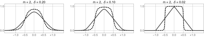
Figure 1. Numerical results for high energy waves with $m=2$: The velocity profile $V_{\delta}$ (black, dashed) approaches as $\delta\to 0$ the indicator function $V_{0}$ while the distance profiles $R_{\delta}$ (gray, solid) converges to the tent map $R_{0}$.

In this note we establish a local uniqueness result for the solitary waves from Proposition 1.

Theorem 3.

Suppose that $\delta_{0}>0$ is sufficiently small, then the solitary waves $R_{\delta},V_{\delta}$ for given $\sigma_{\delta}$ are locally unique for $0<\delta<\delta_{0}$. More precisely, there exists $c_{0}>0$ such that there are no other non-negative, even, and unimodal solutions $(R,V)$ of (2) for fixed $\sigma_{\delta}$ with $|(R,V)-(R_{\delta},V_{\delta})|_{{\mathsf{L}}^{2}}\leq c_{0}$.

Furthermore the family $R,V$ depends continuously on the wave parameter $\sigma$.

The proof is based on an implicit function argument applied to the nonlinear travelling wave operator

(5) $$\mathcal{F}(R,V,{\sigma}_{\delta})=\left(\begin{array}[]{l}\frac{\partial}{\partial x}R(.)-\nabla^{\pm}_{1/2}V(.)\\ \frac{\partial}{\partial x}V(.)-\frac{1}{{\sigma}_{\delta}}\nabla^{\pm}_{1/2}\left(\Phi^{\prime}(R(.))\right)\end{array}\right),$$

where the main challenge is to control the kernel of its linearisation.

3. Linearisation

The linearisation of (5) around a travelling wave ${\left({R_{\delta}},\,{V_{\delta}}\right)}$ with speed ${\sigma}_{\delta}$ reads

(10) $$L_{\delta}\left(\begin{array}[]{l}S(.)\\ W(.)\end{array}\right) =\left(\begin{array}[]{l}\frac{\partial}{\partial x}S(.)-\nabla^{\pm}_{1/2}W(.)\\ \frac{\partial}{\partial x}W(.)-\frac{1}{{\sigma}_{\delta}}\nabla^{\pm}_{1/2}\left(\Phi^{\prime\prime}(R_{\delta}(.))S(.)\right)\end{array}\right)$$

with $\nabla^{\pm}_{1/2}$ being the standard centered-difference operator with spacing $1/2$ . We consider $L_{\delta}$ as an operator on the weighted Sobolev space

$${\mathsf{L}}^{2}_{a}:=\{(S,W):{\mathbb{R}}\to{\mathbb{R}}^{2}:\exp(ax)(S(x),W(x))\in{\mathsf{L}}^{2}({\mathbb{R}},{\mathbb{R}}^{2})\},$$

which is for given parameter $a>0$ defined on the dense subspace

$${\mathsf{H}}^{1}_{a}:=\{(S,W):{\mathbb{R}}\to{\mathbb{R}}^{2}:\exp(ax)(S(x),W(x))\in{\mathsf{H}}^{1}({\mathbb{R}},{\mathbb{R}}^{2})\}.$$

The first important observation is that the shift symmetry of (5) implies that $L_{\delta}$ has at least one kernel function.

Lemma 4.

Let $a>0$ be given, $\delta>0$ be sufficiently small, and $(R_{\delta},V_{\delta})$ be a travelling wave. Then

(11) $${\big{(}{S_{1,\delta}},\,{W_{1,\delta}}\big{)}}:={\left({\frac{dR_{\delta}}{dx}},\,{\frac{dV_{\delta}}{dx}}\right)}$$

is in the kernel of $L_{\delta}$ and belongs to ${\mathsf{H}}^{1}_{a}\cap{\mathsf{H}}^{1}_{-a}$.

Proof.

The identity $L_{\delta}{\big{(}{S_{1,\delta}},\,{W_{1,\delta}}\big{)}}=0$ is obtained by differentiating (2) with respect to $x$. The decay properties follow from ideas in [HR10] as in [HM15, Thm. 10]. ∎

Our main asymptotic result can be formulated as follows and will be proven in several steps.

Proposition 5.

There exists $\delta_{0}>0$ such that

$$\mathrm{ker}\,L_{\delta}=\mathrm{span}\,\left\{{\big{(}{S_{1,\delta}},\,{W_{1,\delta}}\big{)}}\right\}$$

holds for all $0<\delta<\delta_{0}$.

3.1. Prelimenaries

In what follows we denote the wave speed by $c=\sqrt{{\sigma}}$.

Lemma 6.

1. The operator $\nabla^{\pm}_{1/2}$ is invertible on ${\mathsf{L}}^{2}_{a}$ for $a>0$.

2. The operator $L_{\delta}:{\mathsf{H}}^{1}_{a}\to{\mathsf{L}}^{2}_{a}$ is Fredholm for $0<a<a_{c}$, where $a_{c}>0$ is the uniquely determined by $\sinh(a_{c}/2)/(a_{c}/2))=c$.

Proof.

Part (a) follows by Fourier arguments since $\nabla^{\pm}_{1/2}$ acts on ${\mathsf{L}}^{2}_{a}$ as a weighted difference operator . For part (b), the essential spectrum can be calculated explicitly as in [FP04a, Lem. 4.2]. For any $a\in{\mathbb{R}}$, the essential spectrum of $L_{\delta}$ in ${\mathsf{L}}^{2}_{a}$ is given by the following union of two curves:

$$\{\lambda:\lambda=\mathcal{P}_{+}(ik-a)\mbox{ for some }k\in{\mathbb{R}}\}\cup\{\lambda:\lambda=\mathcal{P}_{-}(ik-a)\mbox{ for some }k\in{\mathbb{R}}\},$$

with $\mathcal{P}_{\pm}(\mu)=\mu\pm 2\frac{1}{\sqrt{{\sigma}_{\delta}}}\sinh(\mu/2)$. In particular,

$$\max\{\mbox{Re}\lambda:\lambda\in\sigma_{ess}(L_{\delta})\}=-a+\frac{2}{c}\left|\sinh\left(\frac{a}{2}\right)\right|=:-b_{*}(c,a)<0,$$

so the essential spectrum does not intersect the closed right complex half plane and hence $0$ if and only if $c>1$ and $0<a<a_{c}$, where $a_{c}>0$ is the solution of the given transcendental equation and increases with $c$. As $0$ is not in the essential spectrum $L_{\delta}$, the operator itself is Fredholm. ∎

3.2. Rescaling

We next transform (10) into a second-order advance-delay-differential equation. Letting $S_{\delta}(x)=\exp(-ax)G_{\delta}(x)$ with $G_{\delta}\in{\mathsf{L}}^{2}$ we express the linearised equation as

(12) $$\left(\frac{d}{dx}-a\right)^{2}G_{\delta}=\Delta_{1,-a}\frac{1}{{\sigma}_{\delta}}Q_{\delta}G_{\delta}\,,$$

where the transformed discrete Laplacian is given by

(13) $$\Delta_{1,-a}F(x)=\exp(-a)F(x+1)+\exp(+a)F(x-1)-2F(x)\,.$$

Any solution $G_{\delta}$ to (12) gives immediately a corresponding $S_{\delta}$ and then due to the invertibility of $\nabla^{\pm}_{1/2}$ on ${\mathsf{L}}^{2}_{a}$ also $W_{\delta}$ to obtain a solution of (10).

The key asymptotic observation for the high-energy limit $\delta\to 0$ is that the advance-delay-differential equation (12) implies an effective ODE for both $G_{\delta}$ and $S_{\delta}$ in the vicinity of $x=0$ (‘tip of the tent’ in Fig.1). We therefore rescale the profile $G_{\delta}$ according to

$$x=\delta\tilde{x},\quad\tilde{G}_{\delta}(\tilde{x})=G_{\delta}(\delta\tilde{x}),\quad\tilde{Q}_{\delta}(\tilde{x})=\frac{\delta^{2}}{{\sigma}_{\delta}}Q_{\delta}(\delta\tilde{x}),\quad\frac{d}{d\tilde{x}}=\frac{1}{\delta}\frac{d}{dx}\,.$$

With respect to the new coordinates, (12) becomes

(14) $$\left(\frac{d}{d\tilde{x}}-\delta a\right)^{2}\tilde{G}_{\delta}=\Delta_{1/\delta,-a}{\big{(}\tilde{Q}_{\delta}\tilde{G}_{\delta}\big{)}},$$

where the operator $\Delta_{1/\delta,-a}$ is defined analogously to (13) with spacing $\delta^{-1}$. Moreover, the Green’s function of the differential operator on the left hand side is given by

(15) $$\tilde{H}_{\delta}(\tilde{x})=-\tilde{x}\exp(\delta a\tilde{x})\chi_{(-\infty,0)}(\tilde{x})$$

and the corresponding convolution operator has the following properties.

Lemma 7.

There exists a constant $C>0$ which depends on the parameter $a$ but not on $\delta$ such that for all $\tilde{F}\in{\mathsf{L}}^{2}$ we have

1. $\tilde{H}_{\delta}\ast(\Delta_{1/\delta,-a}\tilde{F})=(\Delta_{1/\delta,-a}\tilde{H}_{\delta})\ast\tilde{F}$,

2. $\delta^{2}\|{\tilde{H}_{\delta}\ast\tilde{F}}\|_{2}+\delta\|{{\left({\tilde{H}_{\delta}\ast\tilde{F}}\right)}^{\prime}}\|_{2}+\|{{\left({\tilde{H}_{\delta}\ast\tilde{F}}\right)}^{\prime\prime}}\|_{2}\leq C\|{\tilde{F}}\|_{2}$,

3. $\delta^{1/2}\|{{\left({\tilde{H}_{\delta}\ast\tilde{F}}\right)}^{\prime}}\|_{\infty}\leq C\|{\tilde{F}}\|_{2}$ and $\|{{\left({\tilde{H}_{\delta}\ast\tilde{F}}\right)}^{\prime}}\|_{\infty}\leq C\|{\tilde{F}}\|_{1}$.

Proof.

Part (i) follows immediately from the Fourier representation of $\Delta_{1/\delta,-a}$ and $\tilde{H}_{\delta}$. In particular, the symbol of $\tilde{H}_{\delta}$ is $h_{\delta}(\tilde{k}):={\left({\mathtt{i}\tilde{k}-\delta a}\right)}^{-2}$, so part (ii) is a direct consequence of Parseval’s inequality. We finally observe that Young’s inequality yields

$$\big{\|}{{\left({\tilde{H}_{\delta}\ast\tilde{F}}\right)}^{\prime}}\big{\|}_{\infty}=\big{\|}{\tilde{H}_{\delta}^{\prime}\ast\tilde{F}}\big{\|}_{\infty}\leq\big{\|}{\tilde{H}_{\delta}^{\prime}\|_{q}\|\tilde{F}}\big{\|}_{p}\quad\mbox{ with }\quad\frac{1}{q}+\frac{1}{p}=1,$$

and hence part (iii) via $\|\tilde{H}_{\delta}^{\prime}\|_{2}\leq C\delta^{-1/2}$ for $p=2$ and $\|\tilde{H}_{\delta}^{\prime}\|_{\infty}\leq C$ for $p=1$. ∎

Our asymptotic analysis strongly relies on the following characterisation of $\tilde{Q}_{\delta}$.

Proposition 8 (properties of the coefficient function).

1. We have

   $$\tilde{Q}_{\delta}(\tilde{x})=\tilde{P}(\tilde{x})+\delta^{m+2}\tilde{Z}_{\delta}(\tilde{x})$$

   where $\tilde{P}$ is even, decays as $\tilde{x}^{-m-2}$ as $\tilde{x}\to\infty$, and does not depend on $\delta$, while the perturbation $\tilde{Z}_{\delta}$ is uniformly bounded in ${\mathsf{L}}^{\infty}$.

2. The solution space of the ODE

   (16) $$\tilde{T}^{\prime\prime}=-2\tilde{P}\tilde{T}$$

   is spanned by an even function $\tilde{T}_{e}$ and an odd function $\tilde{T}_{o}$, which can be normalized by

   $$\tilde{T}_{e}^{\prime}{\left({\tilde{x}}\right)}\quad\xrightarrow{\;\;\tilde{x}\to+\infty\;\;}\quad 1\,,\qquad\tilde{T}_{o}{\left({\tilde{x}}\right)}\quad\xrightarrow{\;\;\tilde{x}\to+\infty\;\;}\quad 1$$

   and satisfy

   $$\sup_{\tilde{x}\in{\mathbb{R}}}{\Big{(}\big{|}{\tilde{T}_{e}^{\prime}{\left({\tilde{x}}\right)}\tilde{x}-\tilde{T}_{e}{\left({\tilde{x}}\right)}}\big{|}+\big{|}{{\left({\tilde{T}_{e}^{\prime}{\left({\tilde{x}}\right)}-1}\right)}\tilde{x}^{m}}\big{|}+\big{|}{\tilde{T}_{o}^{\prime}{\left({\tilde{x}}\right)}\tilde{x}^{m}}\big{|}\Big{)}}\leq C$$

   for some constant $C$ depending on $m$.

Proof.

We refer to [HM15] for the details but mention that the coefficient function $\tilde{P}$ has been constructed from the solution of the nonlinear ODE initial-value problem (4). In a nutshell, we have $\tilde{P}:=\Psi^{\prime\prime}{\left({\tilde{R}_{*}}\right)}$, where $\tilde{R}_{*}$ is the even and asymptotically affine solution to

$$\tilde{R}_{*}^{\prime\prime}=-2\Psi^{\prime}{\left({\tilde{R}_{*}}\right)}\,,\qquad\tilde{R}_{*}{\left({0}\right)}=0\,,\qquad\tilde{R}_{*}{\left({0}\right)}=1$$

with $\Psi^{\prime}{\left({r}\right)}\sim{\left({r}\right)}^{-m-1}$ for large $\left|{r}\right|$. In particular, $\tilde{P}$ has the non-generic property that the odd solution to the linear ODE (16) is asymptotically constant as it is given by $\tilde{T}_{o}=c\tilde{R}_{*}^{\prime}$ for some constant $c$. The remaining assertions on (16) follow from standard ODE arguments and the estimates for $\tilde{Z}_{\delta}$ are provided by an asymptotic analysis of the nonlinear advance-delay-differential equation (2). ∎

Using (15) and Proposition 8 we can finally transform (14) into the fixed point problem

(17) $$\tilde{G}_{\delta}=\tilde{H}_{\delta}\ast{\Big{(}\Delta_{1/\delta,-a}\left(\tilde{P}\tilde{G}_{\delta}+\delta^{m+2}\tilde{Z}_{\delta}\tilde{G}_{\delta}\right)\Big{)}}$$

and are now in the position to characterize the kernel of $L_{\delta}$ by identifying the aforementioned asymptotic ODE.

3.3. Sketch of the proof of Proposition 5

In this section we fix $a>0$, consider families ${\left({\tilde{G}_{\delta}}\right)}_{0<\delta<1}\subset{\mathsf{L}}^{2}$ of solutions to (17), and show that $\tilde{G}_{\delta}$ is – up to normalisation factors and small error terms – uniquely determined.

Compactness: Bootstrapping shows that $\tilde{G}_{\delta}$ is smooth, and without loss of generality we normalise $\tilde{G}_{\delta}$ by

(18) $$\big{|}{\tilde{G}_{\delta}(0)}\big{|}+\|\tilde{P}\tilde{G}_{\delta}\|_{1}+\|\tilde{P}\tilde{G}_{\delta}\|_{2}=1.$$

In view of Lemma 7 – and thanks to (17), $\|{\tilde{Z}_{\delta}}\|_{\infty}\leq C$, and the uniform ${\mathsf{L}}^{p}$-continuity of the operator $\Delta_{1/\delta,-a}$ – we estimate

$$\|{\tilde{G}_{\delta}}\|_{2}\leq C\delta^{-2}\|{\tilde{P}\tilde{G}_{\delta}}\|_{2}+C\delta^{m}\|{\tilde{G}_{\delta}}\|_{2}$$

and obtain $\|{\tilde{G}_{\delta}}\|_{2}\leq C\delta^{-2}$ for all sufficiently small $\delta>0$. Moreover, using Lemma 7 again as well as $m>1$ we find

$$\|{\tilde{G}_{\delta}^{\prime}}\|_{\infty}\leq C{\left({\big{\|}{\tilde{P}\tilde{G}_{\delta}}\big{\|}_{1}+\delta^{m+3/2}\|{\tilde{G}_{\delta}}\|_{2}}\right)}\leq C$$

and

$$\|{\tilde{G}_{\delta}^{\prime\prime}}\|_{2}\leq C{\Big{(}\big{\|}{\tilde{P}\tilde{G}_{\delta}}\big{\|}_{2}+\delta^{m+2}\|{\tilde{G}_{\delta}}\|_{2}\Big{)}}\leq C\,,$$

which in turn give rise to uniform Lipschitz and Hölder estimates for $\tilde{G}_{\delta}$ and $\tilde{G}_{\delta}^{\prime}$, respectively. By the Arzelà-Ascoli theorem we can therefore extract a (not relabeled) subsequence such that $\tilde{G}_{\delta}$ converges in ${\mathsf{BC}}^{1}_{\mathrm{loc}}$ to a limit function $\tilde{G}_{0}$. The bounds for $\tilde{G}_{\delta}(0)$ and $\|{\tilde{G}_{\delta}^{\prime}}\|_{\infty}$ ensure

(19) $$|\tilde{G}_{\delta}(\tilde{x})|\leq 1+C|\tilde{x}|$$

and hence

$$\|\tilde{P}\tilde{G}_{\delta}-\tilde{P}\tilde{G}_{0}\|_{1}\;\;+\;\;\|\tilde{P}\tilde{G}_{\delta}-\tilde{P}\tilde{G}_{0}\|_{2}\quad\xrightarrow{\;\;\delta\to 0\;\;}\quad 0$$

by dominated convergence and due to the tightness of $\tilde{P}$. In particular, the limit $\tilde{G}_{0}$ does not vanish as it also satisfies the normalisation condition (18).

Asymptotic ODE: We next study the functions $\tilde{S}_{\delta}$ with

$$\tilde{S}_{\delta}{\left({\tilde{x}}\right)}:=\exp{\left({-a\delta\tilde{x}}\right)}\tilde{G}_{\delta}{\left({\tilde{x}}\right)}=S_{\delta}{\left({\delta\tilde{x}}\right)}\,,$$

which also converge in ${\mathsf{BC}}^{1}_{\mathrm{loc}}$ to the nontrivial limit $\tilde{S}_{0}=\tilde{G}_{0}$ and satisfy the advance-delay-differential equation

(20) $$\tilde{S}_{\delta}^{\prime\prime}=\Delta_{1/\delta,0}{\Big{(}{\left({\tilde{P}+\delta^{m+2}\tilde{Z}_{\delta}}\right)}\tilde{S}_{\delta}\Big{)}}$$

thanks to (14), where $\Delta_{1/\delta,0}$ abbreviates the discrete Laplacian with spacing $1/\delta$ and standard weights. Combining (20) with the decay of $\tilde{P}$, the uniform bounds for $\tilde{Z}_{\delta}$, as well as the affine bound for $\tilde{G}_{\delta}$ from (19) we obtain

$$\left|{\tilde{S}_{\delta}{\left({\tilde{x}}\right)}}\right|+\left|{\tilde{S}^{\prime}_{\delta}{\left({\tilde{x}}\right)}}\right|\quad\xrightarrow{\;\;\tilde{x}\to+\infty\;\;}\quad 0$$

as well as

$$\left|{\tilde{S}_{\delta}^{\prime\prime}{\left({\tilde{x}}\right)}}\right|\leq C\frac{\exp{\left({-\delta a\tilde{x}}\right)}{\big{(}\tilde{x}+\delta^{-1}\big{)}}}{{\big{(}\tilde{x}-\delta^{-1}\big{)}}^{m+2}}\qquad\text{for}\quad\tilde{x}\geq\tfrac{3}{2}\delta^{-1}$$

and hence

(21) $$\left|{\tilde{S}_{\delta}{\left({\tfrac{3}{2}\delta^{-1}}\right)}}\right|={O{\left({\delta^{m-1}}\right)}}\,,\qquad\left|{\tilde{S}^{\prime}_{\delta}{\left({\tfrac{3}{2}\delta^{-1}}\right)}}\right|={O{\left({\delta^{m}}\right)}}$$

after integration over $\tilde{x}\geq\tfrac{3}{2}\delta^{-1}$. Using the pointwise estimates and the decay of $\tilde{P}$ we further verify

(22) $$\tilde{S}_{\delta}^{\prime\prime}{\left({\tilde{x}}\right)}=-2\tilde{P}{\left({\tilde{x}}\right)}\tilde{S}_{\delta}{\left({\tilde{x}}\right)}+\tilde{E}_{0,\delta}{\left({\tilde{x}}\right)}\qquad\text{for}\quad\tilde{x}\in\tilde{I}_{\delta}:=\left[-\tfrac{1}{2}\delta^{-1},\,+\tfrac{1}{2}\delta^{-1}\right]\,$$

as well as

(23) $$\tilde{S}_{\delta}^{\prime\prime}{\left({\tilde{x}+\delta^{-1}}\right)}=\tilde{P}{\left({\tilde{x}}\right)}\tilde{S}_{\delta}{\left({\tilde{x}}\right)}+\tilde{E}_{+,\delta}{\left({\tilde{x}}\right)}\qquad\text{for}\quad\tilde{x}\in\tilde{I}_{\delta},$$

where the error terms are pointwise of order ${O{\left({\delta^{m}}\right)}}$ and satisfy

(24) $$\int_{\tilde{I}_{\delta}}\left|{\tilde{x}}\right|^{i}{\big{(}\left|{\tilde{E}_{0,\delta}{\left({\tilde{x}}\right)}}\right|+\left|{\tilde{E}_{+,\delta}{\left({\tilde{x}}\right)}}\right|\big{)}}\,\mathrm{d}\tilde{x}={O{\left({\delta^{m-i}}\right)}}\qquad\text{for}\quad i\in\{0,1\}\,.$$

In other words, we can replace the nonlocal equation (20) on the interval $\tilde{I}_{\delta}$ by an asymptotic ODE since both the advance and the delay terms on the right hand side are small, while on the shifted interval $\tilde{I}_{\delta}+\delta^{-1}$ the main contribution stems from the delay term. (On $\tilde{I}_{\delta}-\delta^{-1}$, the advance term is the most relevant one.)

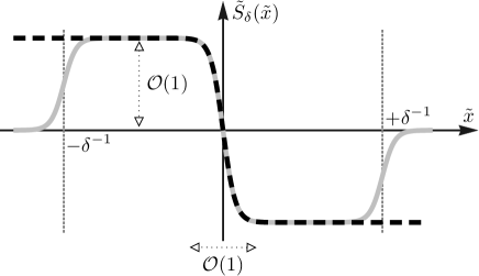
Figure 2. Cartoon of the unique recaled eigenfunction $\tilde{S}_{\delta}$ (gray, solid) and its pointwise limit $\tilde{S}_{0}$ (black, dashed) with respect to the scaled phase variable $\tilde{x}$.

Uniqueness of accumulation points: The linear ODE (22) and the error estimates (24) imply

(25) $$\tilde{S}_{\delta}{\left({\tilde{x}}\right)}=c_{e,\delta}\tilde{T}_{e}{\left({\tilde{x}}\right)}+c_{o,\delta}\tilde{T}_{o}{\left({\tilde{x}}\right)}+{O{\left({\delta^{m-1}}\right)}}\qquad\text{for all}\quad\tilde{x}\in\tilde{I}_{\delta}$$

with $\tilde{T}_{e}$ and $\tilde{T}_{o}$ as in Proposition 8. The constants $c_{e,\delta}$ and $c_{0,\delta}$ are uniquely determined by $\tilde{S}_{\delta}{\left({0}\right)}$ and $\tilde{S}_{\delta}^{\prime}{\left({0}\right)}$, and satisfy

$$\left|{c_{e,\delta}}\right|+\left|{c_{o,\delta}}\right|\quad\xrightarrow{\;\;\delta\to 0\;\;}\quad c\neq 0$$

due to the locally uniform convergence of $\tilde{S}_{\delta}$ and $\tilde{S}_{\delta}^{\prime}$ and the nontriviality of the limit. We further employ the identity

$$\tilde{S}_{\delta}{\left({\tilde{x}}\right)}=\tilde{S}_{\delta}{\left({\tfrac{3}{2}\delta^{-1}}\right)}+\tilde{S}^{\prime}_{\delta}{\big{(}\tfrac{3}{2}\delta^{-1}\big{)}}{\left({\tilde{x}-\tfrac{3}{2}\delta^{-1}}\right)}+\int\limits_{\tilde{x}}^{\tfrac{3}{2}\delta^{-1}}\tilde{S}_{\delta}^{\prime\prime}{\left({\tilde{y}}\right)}{\big{(}\tilde{y}-\tilde{x}\big{)}}\,\mathrm{d}\tilde{y}$$

along with (21) and the asymptotic differential relations (22)+(23) to get

$$\tilde{S}_{\delta}{\left({\tfrac{1}{2}\delta^{-1}}\right)} =\int\limits_{\tfrac{1}{2}\delta^{-1}}^{\tfrac{3}{2}\delta^{-1}}\tilde{S}_{\delta}^{\prime\prime}{\left({\tilde{y}}\right)}{\big{(}\tilde{y}-\tfrac{1}{2}\delta^{-1}\big{)}}\,\mathrm{d}\tilde{y}+{O{\left({\delta^{m-1}}\right)}}$$

$$=\int\limits_{-\tfrac{1}{2}\delta^{-1}}^{+\tfrac{1}{2}\delta^{-1}}\tilde{S}_{\delta}^{\prime\prime}{\left({\tilde{y}+\delta^{-1}}\right)}{\big{(}\tilde{y}+\tfrac{1}{2}\delta^{-1}\big{)}}\,\mathrm{d}\tilde{y}+{O{\left({\delta^{m-1}}\right)}}$$

$$=\int\limits_{-\tfrac{1}{2}\delta^{-1}}^{+\tfrac{1}{2}\delta^{-1}}{\Big{(}-\tfrac{1}{2}c_{e,\delta}\tilde{T}_{e}^{\prime\prime}{\left({\tilde{y}}\right)}-\tfrac{1}{2}c_{o,\delta}\tilde{T}_{o}^{\prime\prime}{\left({\tilde{y}}\right)}\Big{)}}{\big{(}\tilde{y}+\tfrac{1}{2}\delta^{-1}\big{)}}\,\mathrm{d}\tilde{y}+{O{\left({\delta^{m-1}}\right)}}$$

$$=-\frac{c_{e,\delta}}{4\delta}\int\limits_{-\tfrac{1}{2}\delta^{-1}}^{+\tfrac{1}{2}\delta^{-1}}\tilde{T}_{e}^{\prime\prime}{\left({\tilde{y}}\right)}\,\mathrm{d}\tilde{y}-\frac{c_{o,\delta}}{2}\int\limits_{-\tfrac{1}{2}\delta^{-1}}^{+\tfrac{1}{2}\delta^{-1}}\tilde{T}_{o}^{\prime\prime}{\left({\tilde{y}}\right)}\tilde{y}\,\mathrm{d}\tilde{y}+{O{\left({\delta^{m-1}}\right)}}$$

$$=-\frac{c_{e,\delta}}{2\delta}\tilde{T}_{e}^{\prime}{\left({\tfrac{1}{2}\delta^{-1}}\right)}+c_{o,\delta}\tilde{T}_{o}{\left({\tfrac{1}{2}\delta^{-1}}\right)}+{O{\left({\delta^{m-1}}\right)}},$$

where we also used the parity of $\tilde{T}_{e}$ and $\tilde{T}_{o}$ as well as

$$\frac{\,\mathrm{d}missing}{\,\mathrm{d}\tilde{y}}{\Big{(}\tilde{T}_{o}^{\prime}{\left({\tilde{y}}\right)}\tilde{y}-\tilde{T}_{o}{\left({\tilde{y}}\right)}\Big{)}}=\tilde{T}_{o}^{\prime\prime}{\left({\tilde{y}}\right)}\tilde{y},\qquad\tilde{T}^{\prime}_{o}{\left({\tfrac{1}{2}\delta^{-1}}\right)}={O{\left({\delta^{m}}\right)}}.$$

Equating this with (25) evaluated at $\tilde{x}=\tfrac{1}{2}\delta^{-1}$ we arrive at

$$\frac{c_{e,\delta}}{2\delta}{\Big{(}\tilde{T}_{e}^{\prime}{\left({\tfrac{1}{2}\delta^{-1}}\right)}+2\delta\tilde{T}_{e}{\left({\tfrac{1}{2}\delta^{-1}}\right)}\Big{)}}={O{\left({\delta^{m-1}}\right)}}\,.$$

On the other hand, the properties of $\tilde{T}_{e}$ – see again Proposition 8 – provide

$$\tilde{T}_{e}^{\prime}{\left({\tfrac{1}{2}\delta^{-1}}\right)}=2\delta\tilde{T}_{e}{\left({\tfrac{1}{2}\delta^{-1}}\right)}+{O{\left({\delta}\right)}},\qquad\tilde{T}_{e}^{\prime}{\left({\tfrac{1}{2}\delta^{-1}}\right)}=1+{O{\left({\delta^{m}}\right)}}$$

and we conclude that

(26) $$c_{e,\delta}={O{\left({\delta^{m}}\right)}}\,,\qquad c_{o,\delta}=c_{o,0}+{O{\left({\delta^{m}}\right)}},$$

where $c_{o,0}\neq 0$ is uniquely determined by the normalisation condition (18).

Conclusion: In (25) and (26) have shown that $\tilde{S}_{\delta}$ can be approximated with high accuracy by a certain multiple of the odd solution to the linear ODE (16), see Figure 2 for an illustration, and Lemma 6 implies the corresponding asymptotic uniqueness for $\tilde{W}_{\delta}$. In particular, this result applies to the rescaled kernel functions ${\left({\tilde{S}_{1,\delta}},\,{\tilde{W}_{1,\delta}}\right)}$ from (11) as well as to the rescaling of any other solution to $L_{\delta}{\left({S_{\delta}},\,{W_{\delta}}\right)}=0$. If Proposition 5 was false, we would find another solution ${\left({\tilde{S}_{\delta}},\,{\tilde{W}_{\delta}}\right)}$ in the orthogonal ${\mathsf{L}}_{a}^{2}$-complement of ${\left({\tilde{S}_{1,\delta}},\,{\tilde{W}_{1,\delta}}\right)}$ and hence a contradiction.

3.4. Local uniqueness and differentiability of travelling waves

We finally sketch the proof of Theorem 3. We look for solutions of the nonlinear travelling wave equation (5) in ${\mathsf{L}}^{2}_{a}$ and thanks to Lemma 6 we can recover $V$ for given $R$. So it suffices to seek solutions to the second order nonlinear equation

(27) $$\mathcal{F}_{2}(R,{\sigma}_{\delta})=\frac{\partial^{2}}{(\partial x)^{2}}R(.)-\frac{1}{{\sigma}_{\delta}}\Delta_{1}\Phi^{\prime}{\big{(}R(.)\big{)}}=0.$$

We note that $\mathcal{F}_{2}(.,{\sigma}_{\delta}):{\mathsf{H}}^{2}_{a}\to{\mathsf{L}}^{2}_{a}$ maps even to even and odd to odd functions and aim to apply the implicit function theorem to (27). The solutions given in Proposition 1 provide a point with $\mathcal{F}_{2}(R_{\delta},{\sigma}_{\delta})=0$ and the kernel of $L_{\delta}$ is spanned by a single odd profile, see Proposition 5. By Lemma 6 b), $0$ is not in the essential spectrum and this implies that the second order version of $L_{\delta}$ as corresponding to (12) is invertible on the space of even functions. Hence $D_{1}\mathcal{F}_{2}(R,{\sigma}_{\delta})$ is invertible on even functions if $0<\delta<\delta_{0}$. Consequently, the uniqueness part of Theorem 3 is a consequence of the implicit function theorem. Furthermore, $R$ depends smoothly on the wave speed parameter $\sigma$ as long as $\delta$ is small enough such that $\sigma$ will be large. This completes the proof of Theorem 3.

4. Discussion

The control of the kernel of $L_{\delta}$ is an important step to study the dynamical stability of the waves given in Proposition 1. Following [FP04a] it is enough to study eigenfunctions to eigenvalues with non-negative real part of the linearisation of (1) around the travelling waves. The current analysis helps with this as one needs to show that neutral modes are just those $2\times 2$ Jordan blocks that are created due to the symmetry of the system. The symmetry solutions are ${\big{(}{S_{1,\delta}},\,{W_{1,\delta}}\big{)}}$ from (11) and

$${\big{(}{S_{2,\delta}},\,{W_{2,\delta}}\big{)}}:={\left({\frac{dR_{\delta}}{d\delta}},\,{\frac{dV_{\delta}}{d\delta}}\right)}$$

and satisfy the Jordan relations

$$L_{\delta}{\big{(}{S_{1,\delta}},\,{W_{1,\delta}}\big{)}}=0,\qquad L_{\delta}{\big{(}{S_{2,\delta}},\,{W_{2,\delta}}\big{)}}=-\frac{d\sqrt{{\sigma}_{\delta}}}{d\delta}{\big{(}{S_{1,\delta}},\,{W_{1,\delta}}\big{)}}.$$

This programme will be carried out in forth-coming paper for the high-energy limit using a similar combination of techniques of detailed asymptotic analysis and the structure of the underlying equations. Most of the analysis will hold for other potentials than (3) as long as one can guarantee certain non-degeneracy conditions for the energy of a solitary wave. In particular, one needs to show that

$$\frac{dH(R_{\delta},V_{\delta})}{d\delta}\neq 0\quad\mbox{ and }\quad\frac{d\sigma_{\delta}}{d\delta}\neq 0$$

holds in the high-energy limit, where $H$ can be computed using the FPU energy.

Unimodal solitary travelling waves exist following [FW94] for all supersonic wave speeds. They are locally unique and dynamically stable in KdV regime close to the sound speed by [FP99, FP02, FP04a, FP04b]. For the high-energy, i.e. high velocity limit, we have established local uniqueness in this note, whereas results on dynamical stability are forthcoming. We conjecture that for most potentials the whole family of unimodal solitary travelling waves are indeed unique and stable, but new methods need to be developed to understand the linearisation of (1) around the travelling waves for moderate speeds.

References

• [AKJ+15] J. F. R. Archilla, Yu. A. Kosevich, N. Jiménez, V. J. Sánchez-Morcillo, and L. M. García-Raffi. Ultradiscrete kinks with supersonic speed in a layered crystal with realistic potentials. Phys. Rev. E, 91:022912, Feb 2015.
• [FM02] G. Friesecke and K. Matthies. Atomic-scale localization of high-energy solitary waves on lattices. Phys. D, 171(4):211–220, 2002.
• [FP99] G. Friesecke and R. L. Pego. Solitary waves on FPU lattices. I. Qualitative properties, renormalization and continuum limit. Nonlinearity, 12(6):1601–1627, 1999.
• [FP02] G. Friesecke and R. L. Pego. Solitary waves on FPU lattices. II. Linear implies nonlinear stability. Nonlinearity, 15(4):1343–1359, 2002.
• [FP04a] G. Friesecke and R. L. Pego. Solitary waves on Fermi-Pasta-Ulam lattices. III. Howland-type Floquet theory. Nonlinearity, 17(1):207–227, 2004.
• [FP04b] G. Friesecke and R. L. Pego. Solitary waves on Fermi-Pasta-Ulam lattices. IV. Proof of stability at low energy. Nonlinearity, 17(1):229–251, 2004.
• [FSD12] F. Fraternali, L. Senatore, and C. Daraio. Solitary waves on tensegrity lattices. Journal of the Mechanics and Physics of Solids, 60(6):1137 – 1144, 2012.
• [FV99] A.-M. Filip and S. Venakides. Existence and modulation of traveling waves in particle chains. Comm. Pure Appl. Math., 51(6):693–735, 1999.
• [FW94] G. Friesecke and J. A. D. Wattis. Existence theorem for solitary waves on lattices. Comm. Math. Phys., 161(2):391–418, 1994.
• [Her10] M. Herrmann. Unimodal wavetrains and solitons in convex Fermi-Pasta-Ulam chains. Proc. Roy. Soc. Edinburgh Sect. A, 140(4):753–785, 2010.
• [Her17] M. Herrmann. High-energy waves in superpolynomial FPU-type chains. Journal of Nonlinear Science, 2017.
• [HM15] M. Herrmann and K. Matthies. Asymptotic formulas for solitary waves in the high-energy limit of FPU-type chains. Nonlinearity, 28(8):2767–2789, 2015.
• [HR10] M. Herrmann and J. D. M. Rademacher. Heteroclinic travelling waves in convex FPU-type chains. SIAM J. Math. Anal., 42(4):1483–1504, 2010.
• [IJ05] G. Iooss and G. James. Localized waves in nonlinear oscillator chains. Chaos, 15:015113, 2005.
• [Pan05] A. Pankov. Traveling Waves and Periodic Oscillations in Fermi-Pasta-Ulam Lattices. Imperial College Press, London, 2005.
• [SZ09] H. Schwetlick and J. Zimmer. Existence of dynamic phase transitions in a one-dimensional lattice model with piecewise quadratic interaction potential. SIAM J. Math. Anal., 41(3):1231–1271, 2009.
• [Tes01] G. Teschl. Almost everything you always wanted to know about the Toda equation. Jahresber. Deutsch. Math.-Verein., 103(4):149–162, 2001.
• [Tre04] D. Treschev. Travelling waves in FPU lattices. Discrete Contin. Dyn. Syst., 11(4):867–880, 2004.
• [TV14] L. Truskinovsky and A. Vainchtein. Solitary waves in a nonintegrable Fermi-Pasta-Ulam chain. Phys. Rev. E, 90:042903:1–8, 2014.