On the strict monotonicity of the first eigenvalue
of the $p$-Laplacian on annuli

Abstract. Let $B_{1}$ be a ball in $\mathbb{R}^{N}$ centred at the origin and $B_{0}$ be a smaller ball compactly contained in $B_{1}$. For $p\in(1,\infty)$, using the shape derivative method, we show that the first eigenvalue of the $p$-Laplacian in annulus $B_{1}\setminus\overline{B_{0}}$ strictly decreases as the inner ball moves towards the boundary of the outer ball. The analogous results for the limit cases as $p\to 1$ and $p\to\infty$ are also discussed. Using our main result, further we prove the nonradiality of the eigenfunctions associated with the points on the first nontrivial curve of the Fučik spectrum of the $p$-Laplacian on bounded radial domains.

Mathematics Subject Classification (2010): 35J92, 35P30, 35B06, 49R05.
Keywords: $p$-Laplacian, symmetries, shape derivative, Fučik spectrum, eigenvalue, eigenfunction, nonradiality.

1 Introduction

Let $\Omega\subset{\mathbb{R}}^{N}$ be a bounded domain with $N\geq 2$. We consider the following nonlinear eigenvalue problem:

$$\left.\begin{aligned} -\Delta_{p}u&=\lambda|u|^{p-2}u&&{\rm in}\ \Omega,\\ u&=0&&{\rm on}\ \partial\Omega,\end{aligned}\right\}$$ (1.1)

where $\lambda\in\mathbb{R}$ and $\Delta_{p}$ is the $p$-Laplace operator given by $\Delta_{p}u:={\rm div}(|\nabla u|^{p-2}\nabla u)$, $p>1$. A real number $\lambda$ is called an eigenvalue of (1.1) if there exists $u$ in $W^{1,p}_{0}(\Omega)\setminus\{0\}$ satisfying

$$\int_{\Omega}|\nabla u|^{p-2}\,\left<\nabla u,\nabla v\right>{\,\rm d}x=\lambda\int_{\Omega}|u|^{p-2}\,u\,v{\,\rm d}x,\quad\forall\,v\in W^{1,p}_{0}(\Omega),$$

and $u$ is said to be an eigenfunction associated with $\lambda$.

It is well known that (1.1) admits a least positive eigenvalue $\lambda_{1}(\Omega)$ which has the following variational characterization:

$$\lambda_{1}(\Omega)=\inf\left\{\int_{\Omega}|\nabla u|^{p}{\,\rm d}x:u\in W_{0}^{1,p}(\Omega)\setminus\{0\}\text{ with }\left\lVert u\right\rVert_{p}=1\right\}.$$

In this article we consider $\Omega$ of the form $B_{R_{1}}(x)\setminus\overline{B_{R_{0}}(y)}$ with $\overline{B_{R_{0}}(y)}\subset B_{R_{1}}(x)$, where $B_{r}(z)$ denotes the open ball of radius $r>0$ centred at $z\in{\mathbb{R}}^{N}$. Since the $p$-Laplacian is invariant under orthogonal transformations, it can be easily seen that

$$\lambda_{1}(B_{R_{1}}(x)\setminus\overline{B_{R_{0}}(y)})=\lambda_{1}(B_{R_{1}}(0)\setminus\overline{B_{R_{0}}(se_{1})})$$

for any $x,y\in\mathbb{R}^{N}$ such that $|x-y|=s$, where $e_{1}$ is the first coordinate vector. Let the annular region $B_{R_{1}}(0)\setminus\overline{B_{R_{0}}(se_{1})}$ be denoted by $\Omega_{s}$ and let

$$\lambda_{1}(s):=\lambda_{1}(\Omega_{s}).$$

We are interested in the behaviour of $\lambda_{1}(s)$ with respect to $s$ (in other words, with respect to the distance between centres of the inner and outer balls). The main objective of this article is to show that $\lambda_{1}(s)$ is strictly decreasing on $[0,R_{1}-R_{0})$ for any $p>1$.

Apparently the first result in this direction was obtained by Hersch in [16], where he proved (in the case $N=2$, $p=2$ and even for more general annular domains) that $\lambda_{1}(s)$ attains its maximum at $s=0$. In [23], Ramm and Shivakumar conjectured that $\lambda_{1}(s)$ is strictly decreasing and they gave numerical results to support this claim. Later this conjecture and its higher dimensional analogue were proved independently by Harrel et al. [14] and Kesavan [19]. Their proofs mainly rely on the following expression for $\lambda_{1}^{\prime}(s)$ obtained using the Hadamard perturbation formula (see [12, 24]):

$$\lambda_{1}^{\prime}(s)=-\int\limits_{x\in\partial B_{R_{0}}(se_{1})}\left\lvert\frac{\partial u_{s}}{\partial n}(x)\right\rvert^{2}n_{1}(x)\,{\rm dS}(x),$$ (1.2)

where $u_{s}$ is the positive eigenfunction associated with $\lambda_{1}(s)$ with the normalization $\left\lVert u_{s}\right\rVert_{2}=1$, and $n_{1}$ is the first component of $n=(n_{1},\dots,n_{N}),$ the outward unit normal to $\Omega_{s}$. In [14, 19], the authors used the above formula in conjunction with reflection techniques and the strong comparison principle to show that $\lambda_{1}^{\prime}(s)$ is negative on $(0,R_{1}-R_{0})$. For further reading and related open problems on this topic, we refer the reader to the books [2, 15].

For general $p>1,$ it is natural to anticipate that $\lambda_{1}(s)$ is strictly decreasing on $[0,R_{1}-R_{0})$. Indeed, we have the following generalization of formula (1.2):

$$\lambda_{1}^{\prime}(s)=-(p-1)\int\limits_{x\in\partial B_{R_{0}}(se_{1})}\left\lvert\frac{\partial u_{s}}{\partial n}(x)\right\rvert^{p}n_{1}(x)\,{\rm dS}(x).$$ (1.3)

The above expression was derived in [8] using the Hadamard perturbation formula (shape derivative formula) for $\lambda_{1}^{\prime}(s)$ obtained in [13]. However for $p\neq 2$, one lacks a strong comparison principle that guarantee the strict monotonicity of $\lambda_{1}(s).$ More precisely, the strong comparison principle that is applicable for the nonlinear nonhomogeneous problems of the following type:

$$-\Delta_{p}u=\lambda|u|^{p-2}u {\rm in}\ \Omega,\quad u=g {\rm on}\ \partial\Omega.$$ (1.4)

Thus one can not directly extend the ideas of [23, 14, 19] to the nonlinear case and establish the strict monotonicity of $\lambda_{1}(s)$ for general $p>1$. Nevertheless, in [8], Chorwadwala and Mahadevan could show that $\lambda_{1}^{\prime}(s)\leq 0$ for all $s\in[0,R_{1}-R_{0})$ using a weak comparison principle proved in [9] for problems of the form (1.4). However, the authors of [8] could not rule out even the possibility of $\lambda_{1}(s)$ being a constant, due to the absence of the strong comparison principle. In this article, we bypass the usage of the strong comparison principle and prove the following result.

Theorem 1.1.

Let $p\in(1,\infty)$ and let $\lambda_{1}(s)$ be the first eigenvalue of $-\Delta_{p}$ on $\Omega_{s}$. Then

$$\lambda_{1}^{\prime}(0)=0~{}\text{ and }~{}\lambda_{1}^{\prime}(s)<0,\ \forall\,s\in(0,R_{1}-R_{0}).$$

In particular, $\lambda(s)$ is strictly decreasing on $[0,R_{1}-R_{0}).$

For our proof, we derive another formula for $\lambda_{1}^{\prime}(s)$ (in terms of the normal derivative of $u_{s}$ on the outer boundary) in the following form:

$$\lambda_{1}^{\prime}(s)=(p-1)\int\limits_{x\in\partial B_{R_{1}}(0)}\left\lvert\frac{\partial u_{s}}{\partial n}(x)\right\rvert^{p}n_{1}(x)\,{\rm dS}(x).$$ (1.5)

We obtained the above expression by considering the perturbations of $\Omega_{s}$ generated by shifts of the outer ball. On the other hand, formula (1.3) was obtained in [8] by considering the perturbations generated by shifts of the inner ball. If we assume $\lambda_{1}^{\prime}(s)=0$ for some $s\in(0,R_{1}-R_{0})$, then formulas (1.3) and (1.5) help us to show that the first eigenfunction $u_{s}$ associated with $\lambda_{1}(s)$ is radial (up to a translation) in some annular neighbourhoods of the inner and outer boundaries of $\Omega_{s}$. This eventually leads to a contradiction.

Next we study the monotonicity property of the corresponding limit problems. To avoid the ambiguity, for each $p>1,$ here we denote the first eigenvalue $\lambda_{1}(s)$ by $\lambda_{1}(p,s).$ It is known that $\lim\limits_{p\to\infty}\lambda_{1}^{1/p}(p,s)$ and $\lim\limits_{p\to 1}\lambda_{1}(p,s)$ exist, see [17, 18]. We denote the limit functions as below:

$$\Lambda_{\infty}(s):=\lim\limits_{p\to\infty}\lambda_{1}^{1/p}(p,s)\quad\text{and}\quad\Lambda_{1}(s):=\lim\limits_{p\to 1}\lambda_{1}(p,s).$$

Now we state results analogous to Theorem 1.1.

Theorem 1.2.

Let $\Lambda_{\infty}(s)$ and $\Lambda_{1}(s)$ be defined as before. Then $\Lambda_{\infty}(s)$ and $\Lambda_{1}(s)$ are continuous on $[0,R_{1}-R_{0})$ and

1. $\Lambda_{\infty}(s)$ is strictly decreasing on $[0,R_{1}-R_{0})$;

2. $\Lambda_{1}(s)$ is decreasing on $[0,R_{1}-R_{0})$. Moreover, there exists $s^{*}\in[0,R_{1}-R_{0})$ such that $\Lambda_{1}(0)=\Lambda_{1}(s^{*})>\Lambda_{1}(s)$ for all $s\in(s^{*},R_{1}-R_{0})$.

We use a geometric characterization of $\Lambda_{\infty}(s)$ given in [17] for proving part (i), and for the existence of $s^{*}$ in part (ii) we use a variational characterization of $\Lambda_{1}(s)$ given in [18].

Finally, we study the following Fučik eigenvalue problem:

$$\left.\begin{aligned} -\Delta_{p}u&=\alpha(u^{+})^{p-1}-\beta(u^{-})^{p-1}&&\text{in }~{}\Omega,\\ u&=0&&\text{on }~{}\partial\Omega,\end{aligned}\right\}$$ (1.6)

where $\alpha,\beta$ are real numbers (spectral parameters) and $u^{\pm}:=\max\{\pm u,0\}.$ If problem (1.6) possesses a nontrivial solution for some $(\alpha,\beta)$, then we say that $(\alpha,\beta)$ belongs to the Fučik spectrum of (1.6).

In [10], the authors considered a set of critical values $c(t)$ given by

$$c(t):=\inf_{\gamma\in\Gamma}\max_{u\in\gamma[-1,1]}\left(\int\limits_{\Omega}|\nabla u|^{p}\,{\,\rm d}x-t\int\limits_{\Omega}(u^{+})^{p}\,{\,\rm d}x\right),$$ (1.7)

where

$$\Gamma :=\{\gamma\in{\mathcal{C}}([-1,1],{\mathcal{S}}):~{}\gamma(-1)=-\varphi_{1},~{}\gamma(1)=\varphi_{1}\},$$ (1.8)

$${\mathcal{S}} :=\{u\in W_{0}^{1,p}(\Omega):~{}\|u\|_{p}=1\},$$

and $\varphi_{1}$ is the first eigenfunction of (1.1) with the normalization $\|\varphi_{1}\|_{p}=1$. Note that $c(0)=\lambda_{2}(\Omega)$, the second eigenvalue of (1.1). Using $c(t)$, the authors gave a description of the first nontrivial curve $\mathscr{C}$ of the Fučik spectrum of (1.6) as the union of the points $(t+c(t),c(t))$, $t\geq 0$, and their reflections with respect to the diagonal $(t,t)$. Further, they shown that $\mathscr{C}$ is continuous and each eigenfunction associated with a point on $\mathscr{C}$ has exactly two nodal domains (see Theorem 2.1 of [11]).

In [5], Bartsch et al. conjectured that in the linear case ($p=2$) any eigenfunction corresponding to a point on $\mathscr{C}$ is nonradial in a bounded radial domain (i.e., $\Omega$ is a ball or annulus). In the same article, they showed that the conjecture holds in a neighbourhood of $(\lambda_{2}(\Omega),\lambda_{2}(\Omega))$ (see Remark 5.2 of [5]). A complete proof of this conjecture was given by Bartsch and Degiovanni in [4] by estimating generalized Morse indices of corresponding eigenfunctions. In [6], Benedikt et al.  gave a different proof for this conjecture for a ball in ${\mathbb{R}}^{N}$ with $N=2$ and $N=3$. In this article, we provide another proof for this conjecture for any bounded radial domain and even extend this results for general $p\in(1,\infty)$.

Theorem 1.3.

Let $p\in(1,\infty)$ and $\Omega$ be a bounded radial domain in $\mathbb{R}^{N}$, $N\geq 2$. Then any eigenfunction associated with a point on the first nontrivial curve $\mathscr{C}$ of the Fučik spectrum of the problem (1.6) is nonradial.

We obtain the above result as a simple consequence of Theorem 1.1. Moreover, Theorem 1.3 gives a generalization and a simpler proof for Theorem 1.1 of [1] which states the nonradiality of second eigenfunctions of the $p$-Laplacian on a ball.

2 Preliminaries

In this section, we first introduce the reflections with respect to the hyperplanes and the affine hyperplanes. Then we briefly describe the shape derivative formula of [13] and derive the formulas (1.3) and (1.5) for $\lambda_{1}^{\prime}(s)$. Finally we state some results which will be required in the later parts of this article.

For a nonzero vector $a\in\mathbb{R}^{N},$ let $H_{a}$ be the hyperplane perpendicular to $a$, i.e.,

$$H_{a}=\{x\in{\mathbb{R}}^{N}:~{}\left<a,x\right>=0\}.$$

Further, we define the half-spaces

$$\mathcal{H}_{a}^{+}:=\{x\in{\mathbb{R}}^{N}:~{}\left<a,x\right>>0\},\quad\mathcal{H}_{a}^{-}:=\{x\in{\mathbb{R}}^{N}:~{}\left<a,x\right><0\}.$$

Let $\sigma_{a}$ be the reflection with respect to the hyperplane $H_{a}$, i.e.,

$$\sigma_{a}(x)=x-2\frac{\left<a,x\right>}{|a|^{2}}a=x\left[I-2\frac{a^{T}a}{|a|^{2}}\right],\;\forall x\in\mathbb{R}^{N},$$ (2.1)

where the last expression is the matrix product of the vector $x$ and the matrix $\sigma_{a}=I-2\frac{a^{T}a}{|a|^{2}}$. Let $\widetilde{\sigma}_{a}$ be the reflection about the affine hyperplane $se_{1}+H_{a}$. Then $\widetilde{\sigma}_{a}$ is given as below:

$$\widetilde{\sigma}_{a}(x)=x-2\frac{\left<a,x-se_{1}\right>}{|a|^{2}}a=\sigma_{a}(x)+2\frac{\left<a,se_{1}\right>}{|a|^{2}}a.$$

Now we recall the set $\Omega_{s}=B_{R_{1}}(0)\setminus\overline{B_{R_{0}}(se_{1})}$ and for each nonzero vector $a$ in ${\mathbb{R}}^{N}$, consider the following subsets of $\Omega_{s}$:

$$\mathcal{O}^{+}_{a} :=\Omega_{s}\cap\mathcal{H}_{a}^{+};\quad\mathcal{\widetilde{O}}^{+}_{a}:=\Omega_{s}\cap\left(\mathcal{H}_{a}^{+}+se_{1}\right);$$

$$\mathcal{O}^{-}_{a} :=\Omega_{s}\cap\mathcal{H}_{a}^{-};\quad\mathcal{\widetilde{O}}^{-}_{a}:=\Omega_{s}\cap\left(\mathcal{H}_{a}^{-}+se_{1}\right).$$

The relation between some of the subsets of $\overline{\Omega}_{s}$ under the reflections are listed below:

$$\left.\begin{aligned} \sigma_{a}(\mathcal{O}^{+}_{a})&=\mathcal{O}^{-}_{a};\quad\widetilde{\sigma}_{a}(\mathcal{\widetilde{O}}^{+}_{a})=\mathcal{\widetilde{O}}^{-}_{a},\;\forall\,a\in{\mathbb{R}}^{N}\setminus\{0\}\mbox{ with}\left\langle a,e_{1}\right\rangle=0;\\ \sigma_{a}(\mathcal{O}^{+}_{a})&\subset\mathcal{O}^{-}_{a};\quad\widetilde{\sigma}_{a}(\mathcal{\widetilde{O}}^{+}_{a})\subset\mathcal{\widetilde{O}}^{-}_{a},\;\forall\,a\in{\mathbb{R}}^{N}\mbox{ with}\left\langle a,e_{1}\right\rangle>0;\\ \sigma_{a}(\partial B_{R_{0}}(se_{1})\cap\partial\mathcal{O}^{+}_{a})&\subset\mathcal{O}^{-}_{a};\quad\widetilde{\sigma}_{a}(\partial B_{R_{1}}(0)\cap\partial\mathcal{\widetilde{O}}^{+}_{a})\subset\mathcal{\widetilde{O}}^{-}_{a},\;\forall\,a\in{\mathbb{R}}^{N}\mbox{ with}\left\langle a,e_{1}\right\rangle>0;\\ \sigma_{a}(\partial B_{R_{1}}(0)\cap\partial\mathcal{O}^{+}_{a})&=\partial B_{R_{1}}(0)\cap\partial\mathcal{O}^{-}_{a},\;\forall\,a\in{\mathbb{R}}^{N}\setminus\{0\};\\ \widetilde{\sigma}_{a}(\partial B_{R_{0}}(se_{1})\cap\partial\mathcal{\widetilde{O}}^{+}_{a})&=\partial B_{R_{0}}(se_{1})\cap\partial\mathcal{\widetilde{O}}^{-}_{a},\forall\,a\in{\mathbb{R}}^{N}\setminus\{0\}.\end{aligned}\right\}$$ (2.2)

Now for a function $u$ defined on $\overline{\Omega}_{s}$ and for a vector $a\in{\mathbb{R}}^{N}\setminus\{0\}$ with $\left\langle a,e_{1}\right\rangle\geq 0$ we define two new functions $u_{a}:\overline{\mathcal{O}^{+}_{a}}\to{\mathbb{R}}$ and $\widetilde{u}_{a}:\overline{\mathcal{\widetilde{O}}^{+}_{a}}\to{\mathbb{R}}$ as below:

$${u}_{a}(x):=u(\sigma_{a}(x));\quad\widetilde{u}_{a}(x):=u(\widetilde{\sigma}_{a}(x)).$$

By recalling the notation $\sigma_{a}=I-2\frac{a^{T}a}{|a|^{2}}$ from (2.1), for $u\in{\mathcal{C}}^{1}(\overline{\Omega_{s}})$ we see that

$$\nabla u_{a}(x)=\nabla u(\sigma_{a}(x))\sigma_{a},\;\forall x\in\overline{\mathcal{O}^{+}_{a}};\quad\nabla\widetilde{u}_{a}(x)=\nabla u(\widetilde{\sigma}_{a}(x))\sigma_{a},\;\forall x\in\overline{\mathcal{\widetilde{O}}^{+}_{a}}.$$ (2.3)

Further, the normal vector satisfies the following relations:

$$n(\sigma_{a}(x))=n(x)\sigma_{a},\,\forall\,x\in\partial B_{R_{1}}(0)\cap\mathcal{O}^{+}_{a};\quad n(\widetilde{\sigma}_{a}(x))=n(x)\sigma_{a},\,\forall\,x\in\partial B_{R_{0}}(se_{1})\cap\mathcal{O}^{+}_{a}.$$ (2.4)

Shape derivative formulas

For a smooth bounded vector field $V$ on ${\mathbb{R}}^{N}$ consider the perturbation of $\Omega_{s}$ given as $\widetilde{\Omega}_{t}=(I+tV)\Omega_{s}.$ It is known by Theorem 3 of [13] that $\lambda_{1}(t,V):=\lambda_{1}(\widetilde{\Omega}_{t})$ is differentiable at $t=0$ and the derivative is given by

$$\lambda_{1}^{\prime}(0,V):=\lim_{t\rightarrow 0}\frac{\lambda_{1}(t,V)-\lambda_{1}(0,V)}{t}=-(p-1)\int\limits_{\partial\Omega_{s}}\left\lvert\frac{\partial u_{s}}{\partial n}(x)\right\rvert^{p}\left<V(x),n(x)\right>\,{\rm dS},$$ (2.5)

where $n$ is the outward unit normal to $\partial\Omega_{s}$ and ${u_{s}}$ is the first eigenfunction corresponding to $\lambda_{1}(s)$ normalized as

$$u_{s}>0\mbox{ and }\left\lVert u_{s}\right\rVert_{p}=1.$$ (2.6)

In [8], the authors considered the vector field $V$ as given below:

$$V(x)=\rho(x)e_{1},\ \rho\in{\mathcal{C}}_{c}^{\infty}(B_{R_{1}}(0))\ \mbox{and}\ \rho(x)\equiv 1\ \mbox{in a neighbourhood of}\ B_{R_{0}}(se_{1}).$$ (2.7)

For this choice of $V$ and for $t$ sufficiently small, the perturbations $\widetilde{\Omega}_{t}$ of $\Omega_{s}$ are generated by the shifts of the inner ball. More precisely,

$$\widetilde{\Omega}_{t}=\Omega_{s+t}.$$

Therefore, one gets $\lambda_{1}(t,V)=\lambda_{1}(s+t),\lambda_{1}(0,V)=\lambda_{1}(s)$ and hence (2.5) yields

$$\lambda_{1}^{\prime}(s)=-(p-1)\int\limits_{\partial B_{R_{0}}(se_{1})}\left\lvert\frac{\partial u_{s}}{\partial n}(x)\right\rvert^{p}n_{1}(x)\,{\rm dS},$$ (2.8)

where $n_{1}$ is the first component of $n,$ the outward unit normal to $\partial\Omega_{s}$ on $\partial B_{R_{0}}(se_{1})$ (i.e., the inward unit normal to $\partial B_{R_{0}}(se_{1})$).

To derive the expression (1.5) for $\lambda^{\prime}(s)$ (i.e., formula involving the normal derivative of $u_{s}$ on the outer boundary), we consider the perturbations of $\Omega_{s}$ generated by the shifts of the outer boundary. Indeed, such perturbations can be obtained by taking a vector field $V(x)=-\rho(x)e_{1}$ with $\rho\in{\mathcal{C}}^{\infty}({\mathbb{R}}^{N})$ and

1. $\rho=0$ in a neighbourhood of the inner sphere $\partial B_{R_{0}}(se_{1})$;

2. $\rho=1$ in a neighbourhood of the outer sphere $\partial B_{R_{1}}(0)$.

For this choice of $V,$ for $t$ sufficiently close to 0, observe that

$$\widetilde{\Omega}_{t}=B_{R_{1}}(-te_{1})\setminus\overline{B_{R_{0}}(se_{1})}.$$

From the translation invariance of the $p$-Laplacian, we get

$$\lambda_{1}(t,V)=\lambda_{1}\left(B_{R_{1}}(0)\setminus\overline{B_{R_{0}}((s+t)e_{1})}\right)=\lambda_{1}(s+t).$$

Now (2.5) yields

$$\lambda_{1}^{\prime}(s)=\lim_{t\rightarrow 0}\frac{\lambda_{1}(s+t)-\lambda_{1}(t)}{t}=(p-1)\int\limits_{\partial B_{R_{1}}(0)}\left\lvert\frac{\partial u_{s}}{\partial n}(x)\right\rvert^{p}n_{1}(x)\,{\rm dS},$$ (2.9)

where $n_{1}$ is the first component of $n,$ the outward unit normal to $\partial\Omega_{s}$ on $\partial B_{R_{1}}(0)$ (i.e., the outward unit normal to $\partial B_{R_{1}}(0)$).

Next we rewrite the integral in (2.9) using certain symmetries of the domain $\Omega_{s}.$ Set $u=u_{s}$ in (2.9) and express the integral as a sum of two integrals:

$$\int\limits_{\partial B_{R_{1}}(0)}\left\lvert\frac{\partial u}{\partial n}(x)\right\rvert^{p}n_{1}(x)\,{\rm dS}=\int\limits_{\partial B_{R_{1}}(0)\cap\partial\mathcal{O}^{+}_{e_{1}}}\left|\frac{\partial{u}}{\partial n}(x)\right|^{p}n_{1}(x)\,{\rm dS}+\int\limits_{\partial B_{R_{1}}(0)\cap\partial\mathcal{O}^{-}_{e_{1}}}\left|\frac{\partial{u}}{\partial n}(x)\right|^{p}n_{1}(x)\,{\rm dS}.$$ (2.10)

From (2.3) and (2.4) we have $\frac{\partial{u}}{\partial n}(x^{\prime})=\frac{\partial{u_{e_{1}}}}{\partial n}(x)$ and $n_{1}(x^{\prime})=-n_{1}(x)$ on $\partial B_{R_{1}}(0)\cap\mathcal{O}^{+}_{e_{1}},$ where $x^{\prime}=\sigma_{e_{1}}(x).$ Hence, we modify the second integral as below:

$$\int\limits_{\partial B_{R_{1}}(0)\cap\partial\mathcal{O}^{-}_{e_{1}}}\left|\frac{\partial{u}}{\partial n}(x)\right|^{p}n_{1}(x)\,{\rm dS}= \int\limits_{\partial B_{R_{1}}(0)\cap\partial\mathcal{O}^{+}_{e_{1}}}\left|\frac{\partial u}{\partial n}(x^{\prime})\right|^{p}n_{1}(x^{\prime})\,{\rm dS}$$

$$=-\int\limits_{\partial B_{R_{1}}(0)\cap\partial\mathcal{O}^{+}_{e_{1}}}\left|\frac{\partial{u_{e_{1}}}}{\partial n}(x)\right|^{p}n_{1}(x)\,{\rm dS}.$$ (2.11)

Thus, by combining (2.9), (2.10) and (2) we get

$$\lambda_{1}^{\prime}(s)=(p-1)\int\limits_{\partial B_{R_{1}}(0)\cap\partial\mathcal{O}^{+}_{e_{1}}}\left(\left|\frac{\partial u}{\partial n}\right|^{p}-\left|\frac{\partial u_{e_{1}}}{\partial n}\right|^{p}\right)n_{1}\,{\rm dS}.$$ (2.12)

Similarly we can rewrite formula (2.8) as below:

$$\lambda_{1}^{\prime}(s)=-(p-1)\int\limits_{\partial B_{R_{0}}(se_{1})\cap\partial\mathcal{\widetilde{O}}^{+}_{e_{1}}}\left(\left|\frac{\partial u}{\partial n}\right|^{p}-\left|\frac{\partial{\widetilde{u}_{e_{1}}}}{\partial n}\right|^{p}\right)n_{1}\,{\rm dS}.$$ (2.13)

Auxiliary results

Next we state a few results that we require in the subsequent sections. First we recall some results about the regularity of eigenfunctions of (1.1) (cf. Theorem 1.3 of [3]).

Proposition 2.1.

Let $\Omega$ be a smooth domain in ${\mathbb{R}}^{N}$ and let $u$ be a first eigenfunction of (1.1). Then the following assertions are satisfied.

1. $u\in{\mathcal{C}}^{1}(\overline{\Omega}).$

2. $u\in{\mathcal{C}}^{2}(\overline{\Omega_{\delta}}),$ where $\Omega_{\delta}:=\{x\in\Omega:\,\mathrm{dist}(x,\partial\Omega)<\delta\}$ and $|\nabla u|>m>0$ in $\Omega_{\delta}$ for some $m$.

The following version of the strong maximum principle is due to Vazquez (Section 4, [25]).

Proposition 2.2.

Let $\Omega$ be a domain in ${\mathbb{R}}^{N}.$ Let $w\in{\mathcal{C}}^{1}(\overline{\Omega})$ be a positive function satisfying

$$-{\rm div}\left(a_{ij}(x)\frac{\partial w}{\partial x_{j}}\right)\geq 0\mbox{ in }\Omega,$$

where $a_{ij}\in W^{1,\infty}_{loc}(\Omega)$ and there exists $\alpha>0$ such that $a_{ij}(x)\xi_{i}\xi_{j}\geq\alpha|\xi|^{2},\,\forall\,\xi\in{\mathbb{R}}^{N}\setminus\{0\},\,\forall\,x\in\Omega.$ Then

1. $w\equiv 0$ in $\Omega$ or else $w>0$ in $\Omega.$

2. Let $x_{0}$ be a point on $\partial\Omega$ satisfying the interior sphere condition. If $w>0$ in $\Omega$ and $w(x_{0})=0$, then

   $$\frac{\partial w}{\partial n}(x_{0})<0,$$

   where $n$ is the outward unit normal to $\partial\Omega$ at $x_{0}.$

In the next proposition we state a weak comparison result, see Theorem 2.1 and Proposition 4.1 of [9].

Proposition 2.3.

Let $\Omega$ be a domain in ${\mathbb{R}}^{N}$ with Lipschitz boundary. Let $u_{1},u_{2}\in{\mathcal{C}}^{1}(\overline{\Omega})$ be positive weak solutions of $-\Delta_{p}u=\lambda u^{p-1}\mbox{ in }\Omega$. If $u_{1}\geq u_{2}$ on $\partial\Omega,$ then

$$u_{1}\geq u_{2}\mbox{ in }\Omega\mbox{ and }\frac{\partial u_{1}}{\partial n}\leq\frac{\partial u_{2}}{\partial n}\mbox{ on }\{x\in\partial\Omega:\,u_{1}(x)=u_{2}(x)=0\}.$$

3 Main result

In this section we give the proof of Theorem 1.1. We will be considering various annular regions apart from $\Omega_{s}$, for simplicity we denote them as

$$A_{r_{1},r_{0}}(x,y)=B_{r_{1}}(x)\setminus\overline{B_{r_{0}}(y)}.$$

In particular, $A_{R_{1},R_{0}}(0,se_{1})=\Omega_{s}.$ Throughout this section, unless otherwise specified, the eigenfunction $u_{s}$ is the first eigenfunction of $-\Delta_{p}$ on $\Omega_{s}$ normalized as in (2.6), namely $u_{s}>0\mbox{ and }\left\lVert u_{s}\right\rVert_{p}=1.$

The following result is proved in [8] (see Theorem 3.1) using formula (2.13). Here, for the sake of completeness, we present a proof by making use of formula (2.12).

Lemma 3.1.

Let $s\in[0,R_{1}-R_{0})$ and let $\lambda_{1}(s)$ be the first eigenvalue of $-\Delta_{p}$ on $\Omega_{s}$. Then $\lambda^{\prime}(s)\leq 0.$

Proof.

By setting $u=u_{s}$ and noting that $\sigma_{e_{1}}(\mathcal{O}^{+}_{e_{1}})\subset\mathcal{O}^{-}_{e_{1}}$ and $\sigma_{e_{1}}(\partial B_{R_{0}}(se_{1})\cap\partial\mathcal{O}^{+}_{e_{1}})\subset\mathcal{O}^{-}_{e_{1}}$, we easily see that $u_{e_{1}}$ and $u$ weakly satisfy the following problems:

$$\begin{aligned} -\Delta_{p}u_{e_{1}}&=\lambda_{1}(s)\,u_{e_{1}}^{p-1},\\ u_{e_{1}}&=0,\\ u_{e_{1}}&={u},\\ u_{e_{1}}&>0,\end{aligned}\quad\begin{aligned} -\Delta_{p}u&=\lambda_{1}(s)\,u^{p-1}&&\text{ in }\mathcal{O}^{+}_{e_{1}},\\ u&=0&&\text{ on }\partial B_{R_{1}}(0)\cap\partial\mathcal{O}^{+}_{e_{1}},\\ u&={u_{e_{1}}}&&\text{ on }H_{e_{1}}\cap\partial\mathcal{O}^{+}_{e_{1}},\\ u&=0&&\text{ on }\partial B_{R_{0}}(se_{1})\cap\partial\mathcal{O}^{+}_{e_{1}}.\end{aligned}$$

Thus by applying the weak comparison principle (Proposition 2.3) we obtain ${u}_{e_{1}}\geq u$ in $\mathcal{O}^{+}_{e_{1}}$. Moreover, as $u=0$ on $\partial B_{R_{1}}(0)\cap\partial\mathcal{O}^{+}_{e_{1}},$ Proposition 2.2 yields

$$\frac{\partial{u}_{e_{1}}}{\partial n}\leq\frac{\partial u}{\partial n}<0\text{ on }\partial B_{R_{1}}(0)\cap\partial\mathcal{O}^{+}_{e_{1}}.$$ (3.1)

Now since $n_{1}(x)$ is positive for $x\in\partial B_{R_{1}}(0)\cap\partial\mathcal{O}^{+}_{e_{1}}$, from (2.12) and (3.1) we derive that

$$\lambda_{1}^{\prime}(s)=(p-1)\int\limits_{\partial B_{R_{1}}(0)\cap\partial\mathcal{O}^{+}_{e_{1}}}\left(\left|\frac{\partial u}{\partial n}\right|^{p}-\left|\frac{\partial u_{e_{1}}}{\partial n}\right|^{p}\right)n_{1}\,{\rm dS}\;\leq 0.$$

This completes the proof. ∎

Symmetries with respect to the hyperplanes

First we study symmetries of the first eigenfunction of $-\Delta_{p}$ on $\Omega_{s}$. We show that for $s\in(0,R_{1}-R_{0})$ the associated first eigenfunction is symmetric with respect to the hyperplanes perpendicular to $H_{e_{1}}.$

Lemma 3.2.

Let $s\in(0,R_{1}-R_{0})$ and let $u_{s}$ be the first eigenfunction of $-\Delta_{p}$ on $\Omega_{s}.$ If $a\in{\mathbb{R}}^{N}\setminus\{0\}$ with $\left\langle a,e_{1}\right\rangle=0,$ then

$$u_{s}(x)=u_{s}(\sigma_{a}(x)),\,\forall x\in\Omega_{s}.$$

In particular, for $i=2,3,\dots,N$

$$u_{s}(x)=u_{s}(\sigma_{e_{i}}(x))=u_{s}(x_{1},x_{2},\dots,x_{i-1},-x_{i},x_{i+1},\dots,x_{N}),\,\forall x\in\Omega_{s}.$$

Proof.

Clearly for $a\neq 0$ with $\left\langle a,e_{1}\right\rangle=0$, $\mathcal{O}^{+}_{a}=\sigma_{a}(\mathcal{O}^{-}_{a})$ (see (2.2)). Thus $u:=u_{s}$ and $u_{a}:=u_{s}\circ\sigma_{a}$ weakly satisfy the following problems, respectively:

$$\begin{aligned} -\Delta_{p}u_{a}&=\lambda_{1}(s)\,u_{a}^{p-1},\\ u_{a}&=u,\end{aligned}\quad\begin{aligned} -\Delta_{p}u&=\lambda_{1}(s)\,u^{p-1}&&\text{ in }\mathcal{O}^{+}_{a},\\ u&=u_{a}\qquad&&\text{ on }\partial\mathcal{O}^{+}_{a}.\end{aligned}$$

Now by the weak comparison principle (Proposition 2.3), we obtain that ${u}_{a}\equiv u$ in $\mathcal{O}^{+}_{a}$, which implies the desired assertions. ∎

In the next lemma we show that $u_{s}$ is symmetric also with respect to $H_{e_{1}}$ in a neighbourhood of the outer boundary, provided $\lambda_{1}^{\prime}(s)=0.$

Lemma 3.3.

If $\lambda_{1}^{\prime}(s)=0$ for some $s\in(0,R_{1}-R_{0})$, then there exists $r_{1}>0$ such that

$$u_{s}(x)=u_{s}(\sigma_{e_{1}}(x)),\,\forall x\in A_{R_{1},r_{1}}(0,0).$$

Proof.

We set $u=u_{s}$. Since $u\in{\mathcal{C}}^{1}(\overline{\Omega_{s}})$, $u>0$ and $u$ vanishes on $\partial B_{R_{1}}(0)$ and $\partial B_{R_{0}}(se_{1}),$ there exists $r^{*}\in(R_{0}+s,R_{1})$ such that $\frac{\partial u}{\partial x_{1}}(r^{*}e_{1})=0$. Define

$$r_{1}=\sup\left\{\left\lvert x\right\rvert>0:\,\left<\nabla u(x),x\right>=0\right\}.$$ (3.2)

As $\frac{\partial u}{\partial n}(x)<0$ on $\partial B_{R_{1}}(0)$ (by Proposition 2.2), $\left\langle\nabla u(x),x\right\rangle<0$ in a neighbourhood of $\partial B_{R_{1}}(0).$ Thus clearly $r_{1}\in[r^{*},R_{1}).$ By the construction, $A_{R_{1},r_{1}}(0,0)$ is the maximal annular neighbourhood of $\partial B_{R_{1}}(0)$ on which $\left<\nabla u(x),x\right>$ is nonvanishing. Further, by the continuity of $\nabla u$ there must exist $x_{1}\in\partial B_{r_{1}}(0)$ such that

$$\left<\nabla u(x_{1}),x_{1}\right>=0.$$ (3.3)

Set $u_{e_{1}}=u\circ\sigma_{e_{1}}$ on $A_{R_{1},r_{1}}(0,0)\cap\mathcal{O}_{e_{1}}^{+}.$ To show $u\equiv u_{e_{1}}$ we linearise the $p$-Laplacian on the domain $A_{R_{1},r}(0,0)\cap\mathcal{O}_{e_{1}}^{+}$ with $r_{1}<r<R_{1}$ by setting $w={u}_{e_{1}}-u$. Then $w$ weakly satisfies the following problem:

$$-\mbox{div}(A(x)\nabla w) =\lambda\left({u}_{e_{1}}^{p-1}-u^{p-1}\right)\geq 0 \mbox{ in }A_{R_{1},r}(0,0)\cap\mathcal{O}^{+}_{e_{1}},$$

$$w \geq 0 \mbox{ on }\partial(A_{R_{1},r}(0,0)\cap\mathcal{O}^{+}_{e_{1}}),$$

where the coefficient matrix $A(x)=[a_{ij}(x)]$ is given by

$$a_{ij}(x) =\int\limits_{0}^{1}|(1-t)\nabla u(x)+t\nabla u_{e_{1}}(x)|^{p-2}$$

$$\times\left[I+(p-2)\frac{\left[(1-t)\nabla u(x)+t\nabla u_{e_{1}}(x)]^{T}[(1-t)\nabla u(x)+t\nabla u_{e_{1}}(x)\right]}{|(1-t)\nabla u(x)+t\nabla u_{e_{1}}(x)|^{2}}\right]_{ij}{\rm d}t.$$

Now we show that $A(x)$ is uniformly positive definite on $A_{R_{1},r}(0,0)\cap\mathcal{O}_{e_{1}}^{+}.$ Since $\left<\nabla u(x),x\right>$ does not vanish on $A_{R_{1},r_{1}}(0,0)$ and is negative near the boundary $\partial B_{R_{1}}(0)$, we see that $\left<\nabla u(x),x\right><0$ in $A_{R_{1},r}(0,0).$ By the continuity, we can find $\delta_{r}>0$ such that

$$\left<\nabla u(x),x\right><-\delta_{r}\text{ in }A_{R_{1},r}(0,0).$$

Notice that $\left<\nabla u_{e_{1}}(x),x\right>=\left<\nabla(u(\sigma_{e_{1}}(x))),x\right>=\left<\nabla u(\sigma_{e_{1}}(x))\sigma_{e_{1}},x\right>=\left<\nabla u(\sigma_{e_{1}}(x)),\sigma_{e_{1}}(x)\right>.$ Thus, by the above inequality we have $\left<\nabla u_{e_{1}}(x),x\right><-\delta_{r}\text{ in }A_{R_{1},r}(0,0)\cap\mathcal{O}^{+}_{e_{1}}.$ Therefore,

$$(1-t)\left<\nabla u(x),x\right>+t\left<\nabla u_{e_{1}}(x),x\right><-\delta_{r},\forall t\in[0,1],\forall x\in A_{R_{1},r}(0,0)\cap\mathcal{O}^{+}_{e_{1}}.$$

Hence, for $x\in A_{R_{1},r}(0,0)$ we get

$$\left|(1-t)\nabla u(x)+t\nabla{u}_{e_{1}}(x)\right|\geq\left|\left<(1-t)\nabla u(x)+t\nabla{u}_{e_{1}}(x),\frac{x}{|x|}\right>\right|>\frac{\delta_{r}}{R_{1}}=m_{r}.$$ (3.4)

Further, since $|\nabla u|$ is bounded in $A_{R_{1},r}(0,0)$, there exists $M_{r}>0$ such that

$$\left|(1-t)\nabla u(x)+t\nabla{u}_{e_{1}}(x)\right|\leq M_{r}.$$ (3.5)

Note that for each $a\in{\mathbb{R}}^{N}\setminus\{0\},$ the matrix $a^{T}a$ has eigenvalues $\{0,|a|^{2}\}.$ Thus, for any $y\in{\mathbb{R}}^{N},$

$$\min\{1,p-1\}|a|^{p-2}|y|^{2}\leq\left\langle|a|^{p-2}\left[I+(p-2)\frac{a^{T}a}{|a|^{2}}\right]y,y\right\rangle\leq\max\{1,p-1\}|a|^{p-2}|y|^{2}.$$ (3.6)

From (3.4), (3.5) and (3.6), for $x\in A_{R_{1},r}(0,0)$ and $y\in{\mathbb{R}}^{N}$ we obtain

$$\left\langle A(x)y,y\right\rangle\geq\left\{\begin{array}[]{ll}m_{r}^{p-2}|y|^{2}&\mbox{ for }p\geq 2,\\ (p-1)M_{r}^{p-2}|y|^{2}&\mbox{ for }1<p<2.\end{array}\right.$$

Thus the differential operator in (3) defined by means of $A(x)$ is uniformly elliptic in $A_{R_{1},r}(0,0).$ Moreover, by Proposition 2.1, $a_{ij}\in{\mathcal{C}}^{1}({A_{R_{1},r}(0,0)})$. Hence, the strong maximum principle for (3) (Proposition 2.2) implies that either $w\equiv 0$, or $w>0$ in $A_{R_{1},r}(0,0)\cap\mathcal{O}^{+}_{e_{1}}$. Moreover, if $w>0$ in $A_{R_{1},r}(0,0)\cap\mathcal{O}^{+}_{e_{1}}$, then

$$\frac{\partial{u}_{e_{1}}}{\partial n}-\frac{\partial u}{\partial n}=\frac{\partial w}{\partial n}<0\text{ on }\partial B_{R_{1}}(0)\cap\partial\mathcal{O}_{e_{1}}.$$

Now (2.12) together with the above inequality implies that $\lambda_{1}^{\prime}(s)<0$, which contradicts our assumption $\lambda_{1}^{\prime}(s)=0$. Thus we must have $w\equiv 0$ and hence $u\equiv u_{e_{1}}$ in $A_{R_{1},r}(0,0)\cap\mathcal{O}^{+}_{e_{1}}$. Since $r\in(r_{1},R_{1})$ is arbitrary, we conclude that $u(x)=u(\sigma_{e_{1}}(x)),\;\forall x\in A_{R_{1},r_{1}}(0,0)$. ∎

Next we show that $u$ is symmetric in $A_{R_{1},r_{1}}(0,0)$ with respect to all the hyperplanes.

Lemma 3.4.

Let $s$ and $r_{1}$ be as in Lemma 3.3. Then for any nonzero vector $a\in{\mathbb{R}}^{N}$

$$u_{s}(x)=u_{s}(\sigma_{a}(x)),\,\forall x\in A_{R_{1},r_{1}}(0,0).$$

Proof.

The case $\left\langle a,e_{1}\right\rangle=0$ follows from Lemma 3.2. Note that $\sigma_{a}(x)=\sigma_{ka}(x)$ for $k\in{\mathbb{R}}\setminus\{0\}.$ Thus, it is enough to prove the result for $a\in A_{R_{1},r_{1}}(0,0)$ with $\left\langle a,e_{1}\right\rangle>0.$ In this case we have $\sigma_{a}(\mathcal{O}^{+}_{a})\subset\mathcal{O}^{-}_{a}$. Now by setting $u=u_{s}$ and $u_{a}=u_{s}\circ\sigma_{a}$ we see that $u_{a}$ and $u$ satisfy the following problems in $\mathcal{O}^{+}_{a}$:

$$\begin{aligned} -\Delta_{p}u_{a}&=\lambda_{1}(s)\,u_{a}^{p-1},\\ u_{a}&=0,\\ u_{a}&={u},\\ u_{a}&>0,\end{aligned}\quad\begin{aligned} -\Delta_{p}u&=\lambda_{1}(s)\,u^{p-1}&&\text{ in }\mathcal{O}^{+}_{a},\\ u&=0&&\text{ on }\partial B_{R_{1}}(0)\cap\partial\mathcal{O}^{+}_{a},\\ u&={u_{a}}&&\text{ on }H_{a}\cap\partial\mathcal{O}^{+}_{a},\\ u&=0&&\text{ on }\partial B_{R_{0}}(se_{1})\cap\partial\mathcal{O}^{+}_{a}.\end{aligned}$$

Applying the weak comparison principle (Proposition 2.3), we obtain that ${u}_{a}\geq u$ in $\mathcal{O}^{+}_{a}$. As before we set $w=u_{a}-u.$ From Lemma 3.2 and Lemma 3.3 we obtain $u(a)=u(-a)$ as below:

$$u(a_{1},a_{2},\dots,a_{N}) =u(a_{1},-a_{2},\dots,a_{N})$$

$$=\dots=u(a_{1},-a_{2},\dots,-a_{N})=u(-a_{1},-a_{2},\dots,-a_{N}).$$

By definition $u_{a}(a)=u(-a)$ and hence $w(a)=0$. Now we proceed along the same lines as in Lemma 3.3 and see that $w$ satisfies the following problem:

$$-{\rm div}(A(x)w)\geq 0\mbox{ in }A_{R_{1},r}(0,0)\cap\mathcal{O}^{+}_{a};\quad w\geq 0\mbox{ on }\partial(A_{R_{1},r}(0,0)\cap\mathcal{O}^{+}_{a})$$

for any $r\in(r_{1},R_{1})$, where the coefficient matrix $A(x)$ is uniformly positive definite. By the strong maximum principle we have either $w\equiv 0$ or else $w>0$ in $A_{R_{1},r}(0,0)\cap\mathcal{O}^{+}_{a}.$ Since $w(a)=0,$ we obtain $w\equiv 0$ and hence $u\equiv u_{a}$ in $A_{R_{1},r}(0,0)\cap\mathcal{O}^{+}_{a}.$ Finally, using the reflection, we conclude that $u(x)=u(\sigma_{a}(x)),$ $\forall\,x\in A_{R_{1},r_{1}}(0,0).$ ∎

Theorem 3.5.

Let $s\in(0,R_{1}-R_{0})$ and let $u_{s}$ be the first eigenfunction of $-\Delta_{p}$ on $\Omega_{s}.$ If $\lambda_{1}^{\prime}(s)=0$, then $u_{s}$ is radial in the annulus $A_{R_{1},r_{1}}(0,0),$ where $r_{1}$ is given by Lemma 3.3. Furthermore, $\nabla u_{s}=0$ on $\partial B_{r_{1}}(0)$.

Proof.

Let $b,c\in A_{R_{1},r_{1}}(0,0)$ be such that $b\neq c$ and $|b|=|c|.$ Then there exists a constant $k$ such that $a=k(b-c)\in A_{R_{1},r_{1}}(0,0).$ Noting that $\sigma_{a}(b)=c,$ from Lemma 3.4 we obtain that

$$u_{s}(b)=u_{s}(\sigma_{a}(b))=u_{s}(c).$$

Since $b$ and $c$ are arbitrary, we conclude that $u_{s}$ is radial in the annulus $A_{R_{1},r_{1}}(0,0)$. Further, as $u_{s}$ is continuously differentiable in $A_{R_{1},r_{1}}(0,0)$ and $\nabla u_{s}(x_{1})\cdot x_{1}=0$ (see (3.3)), the radiality of $u_{s}$ gives $\nabla u_{s}=0$ on $\partial B_{r_{1}}(0)$. ∎

Symmetries with respect to the affine hyperplanes passing through $se_{1}$

In this subsection we prove the radiality (up to a translation of the origin) of $u_{s}$ in a neighbourhood of the inner boundary. Since $\widetilde{\sigma}_{a}(x)={\sigma}_{a}(x)$ for $a$ such that $\left\langle a,e_{1}\right\rangle=0$, Lemma 3.2 holds as it is, and hence we have for $i=2,\dots,N$

$$u_{s}(x)=u_{s}(\widetilde{\sigma}_{e_{i}}(x))=u(x_{1},x_{2},\dots,x_{i-1},-x_{i},x_{i+1},\dots,x_{N}),\,\forall x\in\Omega_{s}.$$

Next we prove a symmetry result along the same lines as in Lemma 3.3.

Lemma 3.6.

Let $s\in(0,R_{1}-R_{0})$ and let $u_{s}$ be the first eigenfunction of $-\Delta_{p}$ on $\Omega_{s}.$ If $\lambda_{1}^{\prime}(s)=0$, then there exists $r_{0}>0$ such that

$$u_{s}(x)=u(\widetilde{\sigma}_{e_{1}}(x))=u_{s}(-x_{1}+2s,x_{2},\dots,x_{N}),\,\forall x\in A_{r_{0},R_{0}}(se_{1},se_{1}).$$

Proof.

As it was shown in the proof of Lemma 3.3, we have $r^{*}\in(R_{0}+s,R_{1})$ such that $\frac{\partial u}{\partial x_{1}}(r^{*}e_{1})=0$. Define

$$r_{0}=\inf\left\{\left\lvert x-se_{1}\right\rvert>0:\,\left<\nabla u(x),x-se_{1}\right>=0\right\}.$$ (3.7)

Clearly $r_{0}\in(R_{0},R_{1}-s),$ since by Hopf’s maximum principle $\left<\nabla u(x),x-se_{1}\right>=|x-se_{1}|\frac{\partial u}{\partial n}(x)\neq 0$ on $\partial B_{R_{0}}(se_{1})$. By the construction, $A_{r_{0},R_{0}}(se_{1},se_{1})$ is the maximal annular neighbourhood of $\partial B_{R_{0}}(se_{1})$ on which $\left<\nabla u(x),x-se_{1}\right>$ is nonvanishing. Further, by the continuity of $\nabla u$ there must exist $x_{0}\in\partial B_{r_{0}}(se_{1})$ such that

$$\left<\nabla u(x_{0}),x_{0}-se_{1}\right>=0.$$

As in the proof of Lemma 3.3, we linearise the $p$-Laplacian on the domain $A_{r,R_{0}}(se_{1},se_{1})\cap\widetilde{\mathcal{O}}_{e_{1}}^{+}$ with $R_{0}<r<r_{0}$ by setting $w={\widetilde{u}}_{e_{1}}-u$. Then $w$ weakly satisfies the following problem:

$$-\mbox{div}(A(x)\nabla w) =\lambda\left({\widetilde{u}}_{e_{1}}^{p-1}-u^{p-1}\right)\geq 0 \mbox{ in }A_{r,R_{0}}(se_{1},se_{1})\cap\widetilde{\mathcal{O}}_{e_{1}}^{+},$$

$$w \geq 0 \mbox{ on }\partial(A_{r,R_{0}}(se_{1},se_{1})\cap\widetilde{\mathcal{O}}_{e_{1}}^{+}).$$

By similar arguments as in Lemma 3.3, the above differential operator is uniformly elliptic on $A_{r,R_{0}}(se_{1},se_{1})\cap\widetilde{\mathcal{O}}_{e_{1}}^{+}$ and hence by the strong maximum principle we have either $w\equiv 0$ or $w>0$ on this domain. If $w>0$ in $A_{r,R_{0}}(se_{1},se_{1})\cap\widetilde{\mathcal{O}}_{e_{1}}^{+}$, then by the Hopf maximum principle

$$\frac{\partial{\widetilde{u}}_{e_{1}}}{\partial n}-\frac{\partial u}{\partial n}=\frac{\partial w}{\partial n}<0\text{ on }\partial B_{R_{0}}(se_{1})\cap\partial\widetilde{\mathcal{O}}_{e_{1}}^{+}.$$

Now (2.13) implies that $\lambda_{1}^{\prime}(s)<0$, a contradiction to the assumption $\lambda_{1}^{\prime}(s)=0$. Thus we must have $w\equiv 0$ and hence $u\equiv\widetilde{u}_{e_{1}}$ in $A_{r,R_{0}}(se_{1},se_{1})\cap\widetilde{\mathcal{O}}_{e_{1}}^{+}.$ Since $r\in(R_{0},r_{0})$ is arbitrary, we obtain the desired fact. ∎

Next we state a lemma which is a counterpart of Lemma 3.4. The proof follows along the same lines.

Lemma 3.7.

Let $s\in(0,R_{1}-R_{0})$ and let $u_{s}$ be the first eigenfunction of $-\Delta_{p}$ on $\Omega_{s}.$ If $\lambda_{1}^{\prime}(s)=0$, then for any nonzero vector $a\in{\mathbb{R}}^{N}$

$$u_{s}(x)=u_{s}(\widetilde{\sigma}_{a}(x)),\,\forall x\in A_{r_{0},R_{1}}(se_{1},se_{1}),$$

where $r_{0}$ is given by Lemma 3.6.

The next theorem, which is a counterpart of Theorem 3.5, states that $u_{s}$ is radial (up to a translation of the origin) in a neighbourhood of the inner ball. The proof follows along the same lines using Lemma 3.2, Lemma 3.6 and Lemma 3.7.

Theorem 3.8.

Let $s\in(0,R_{1}-R_{0})$ and let $u_{s}$ be the first eigenfunction of $-\Delta_{p}$ on $\Omega_{s}.$ If $\lambda_{1}^{\prime}(s)=0$, then $u_{s}$ is radial in the annulus $A_{r_{0},R_{0}}(se_{1},se_{1}).$ Furthermore, $\nabla u_{s}=0$ on $\partial B_{r_{0}}(se_{1})$.

Remark 3.9.

Let $u_{0}$ be a positive first eigenfunction of $-\Delta_{p}$ on $A_{R_{1},R_{0}}(0,0).$ Note that $u_{0}$ is radial (cf. [21, Proposition 1.1]) and one can verify that $u_{0}$ attains its maximum on a unique sphere of radius $\bar{r}\in(R_{0},R_{1})$ and $u_{0}^{\prime}(\bar{r})=0.$ From the simiplicity of the first eigenvalue, it is clear that every first eigenfunction $u$ of $-\Delta_{p}$ on $A_{R_{1},R_{0}}(0,0)$ is radial and $u^{\prime}(\bar{r})=0.$

Lemma 3.10.

Let $\lambda_{1}^{\prime}(s)=0$ for some $s\in(0,R_{1}-R_{0})$. Let $r_{0}$ and $r_{1}$ be given by Lemmas 3.2 and 3.6, respectively. Then $r_{0}=r_{1}=\bar{r}.$

Proof.

From the definitions of $r_{0}$ and $r_{1}$ (see (3.7) and (3.2)) it easily follows that $r_{0}\leq r_{1}.$ First we show that $r_{1}\leq\bar{r}$. Suppose that $r_{1}>\bar{r}$. For notational simplicity, we denote an annular region with centre at the origin as $A_{t_{1},t_{0}}=A_{t_{1},t_{0}}(0,0)$. Now consider the following function on $A_{R_{1},R_{0}}$:

$$w_{1}(x)=\left\{\begin{aligned} &u_{s}(x),&&x\in A_{R_{1},r_{1}},\\ &C_{1},&&x\in A_{r_{1},\bar{r}},\\ &u_{0}(x),&&x\in A_{\bar{r},R_{0}},\end{aligned}\right.$$

where $C_{1}=u_{s}(x)$ for $|x|=r_{1}.$ By multiplying with an appropriate constant we can choose $u_{0}$ in such a way that $u_{0}(x)=C_{1}$ for $|x|=\bar{r}.$ Since $w_{1}$ is continuous and piecewise differentiable on $A_{R_{1},R_{0}}$ we have $w_{1}\in W_{0}^{1,p}(A_{R_{1},R_{0}})$. To estimate $\left\lVert\nabla w_{1}\right\rVert_{p}^{p}$, we derive a few identities. Note that for any $r\in(r_{1},R_{1}),$ $\nabla u_{s}$ does not vanish on $A_{R_{1},r}$ and hence $u_{s}\in{\mathcal{C}}^{2}(A_{R_{1},r})$, see Proposition 2.1. Thus $u_{s}\in{\mathcal{C}}^{2}(A_{R_{1},r_{1}})$ and hence the following equation holds pointwise in $A_{R_{1},r_{1}}:$

$$-\Delta_{p}u_{s}=\lambda_{1}(s)|u_{s}|^{p-2}u_{s}.$$

Multiply the above equation by $u_{s}$ and integrate over $A_{R_{1},r_{1}}$ to get

$$\int\limits_{A_{R_{1},r_{1}}}-\Delta_{p}u_{s}\;u_{s}{\,\rm d}x=\lambda_{1}(s)\int\limits_{A_{R_{1},r_{1}}}|u_{s}|^{p-2}u_{s}\,u_{s}{\,\rm d}x.$$

Now by noting that $\nabla u_{s}=0$ on $\partial B_{r_{1}}(0)$ and $u_{s}=0$ on $\partial B_{R_{1}}(0)$, the integration by parts gives

$$\int\limits_{A_{R_{1},r_{1}}}|\nabla u_{s}|^{p}{\,\rm d}x=\lambda_{1}(s)\int\limits_{A_{R_{1},r_{1}}}|u_{s}|^{p}{\,\rm d}x.$$ (3.8)

Similarly

$$\int\limits_{A_{\bar{r},R_{0}}}|\nabla u_{0}|^{p}{\,\rm d}x=\lambda_{1}(0)\int\limits_{A_{\bar{r},R_{0}}}|u_{0}|^{p}{\,\rm d}x.$$ (3.9)

Now we estimate $\left\lVert\nabla w_{1}\right\rVert_{p}^{p}$:

$$\int\limits_{A_{R_{1},R_{0}}}|\nabla w_{1}|^{p}{\,\rm d}x =\int\limits_{A_{R_{1},r_{1}}}|\nabla u_{s}|^{p}{\,\rm d}x+\int\limits_{A_{\bar{r},R_{0}}}|\nabla u_{0}|^{p}{\,\rm d}x.$$

By using (3.8) and (3.9) and inequality $\lambda_{1}(s)\leq\lambda_{1}(0)$ we obtain

$$\int\limits_{A_{R_{1},R_{0}}}|\nabla w_{1}|^{p}{\,\rm d}x\leq\lambda_{1}(0)\left(\int\limits_{A_{R_{1},r_{1}}}|u_{s}|^{p}{\,\rm d}x+\int\limits_{A_{\bar{r},R_{0}}}|u_{0}|^{p}{\,\rm d}x\right).$$

Next we estimate $\left\lVert w_{1}\right\rVert_{p}^{p}$:

$$\displaystyle\int\limits_{A_{R_{1},R_{0}}}|w_{1}|^{p}{\,\rm d}x =\int\limits_{A_{R_{1},r_{1}}}|u_{s}|^{p}{\,\rm d}x+\int\limits_{A_{r_{1},\bar{r}}}C_{1}^{p}{\,\rm d}x+\int\limits_{A_{\bar{r},R_{0}}}|u_{0}|^{p}{\,\rm d}x$$

$$>\int\limits_{A_{R_{1},r_{1}}}|u_{s}|^{p}{\,\rm d}x+\int\limits_{A_{\bar{r},R_{0}}}|u_{0}|^{p}{\,\rm d}x.$$

Now combining the above estimates, we arrive at

$$\int\limits_{A_{R_{1},R_{0}}}|\nabla w_{1}|^{p}{\,\rm d}x<\lambda_{1}(0)\int\limits_{A_{R_{1},R_{0}}}|w_{1}|^{p}{\,\rm d}x,$$

a contradiction to the definition of $\lambda_{1}(0)$. Hence we must have $r_{1}\leq\bar{r}.$
Next we show that $\bar{r}\leq r_{0}.$ Suppose that $\bar{r}>r_{0}.$ In this case, we define $w_{2}$ on $A_{R_{1},R_{0}}$ as below:

$$w_{2}(x)=\left\{\begin{aligned} &u_{0}(x),&&x\in A_{R_{1},\bar{r}},\\ &C_{2},&&x\in A_{\bar{r},r_{0}},\\ &u_{s}(x+se_{1}),&&x\in A_{r_{0},R_{0}},\end{aligned}\right.$$

where $C_{2}=u_{s}(x)$ for $|x+se_{1}|=r_{0}$ and $u_{0}$ is scaled to satisfy $u_{0}(x)=C_{2}$ for $|x|=\bar{r}.$ As before we see that $w_{2}\in W^{1,p}_{0}(A_{R_{1},R_{0}})$ and

$$\int\limits_{A_{R_{1},R_{0}}}|\nabla w_{2}|^{p}{\,\rm d}x<\lambda_{1}(0)\int\limits_{A_{R_{1},R_{0}}}|w_{2}|^{p}{\,\rm d}x,$$

which again contradicts the definition of $\lambda_{1}(0).$ Thus $\bar{r}\leq r_{0}$ and we conclude that $r_{0}=\bar{r}=r_{1}.$ ∎

Now we give a proof of our main theorem.

Proof of Theorem 1.1:
Suppose that there exists $s>0$ such that $\lambda_{1}^{\prime}(s)=0$. Now Lemmas 3.2, 3.6 and 3.10 give $r_{0}$ and $r_{1}$ with $r_{0}=r_{1}$. Further, from the definitions of $r_{0}$ and $r_{1}$ (see (3.7) and (3.2)) we can deduce that

$$\nabla u((r_{0}+s)e_{1})=0\mbox{ and }\nabla u(re_{1})\neq 0,\,\forall r>r_{1}.$$

This is a contradiction, since $r_{0}+s=r_{1}+s>r_{1}.$ Thus $\lambda_{1}^{\prime}(s)<0$ for all $s\in(0,R_{1}-R_{0}).$ ∎

Remark 3.11.

Note that in Theorem 1.1 we consider only the case $\overline{B_{R_{0}}(se_{1})}\subset B_{R_{1}}(0)$, i.e., $s\in[0,R_{1}-R_{0})$. For any $s_{1},s_{2}$ satisfying $\sqrt{R_{1}^{2}-R_{0}^{2}}\leq s_{1}<s_{2}\leq R_{1}+R_{0}$, it is geometrically evident that

$$B_{R_{1}}(0)\setminus\overline{B_{R_{0}}(s_{1}e_{1})}\subsetneq B_{R_{1}}(0)\setminus\overline{B_{R_{0}}(s_{2}e_{1})}.$$

Now the strict domain monotonicity of $\lambda_{1}(s)$ (cf. Lemma 5.7 of [10]) gives $\lambda_{1}(s_{1})>\lambda_{1}(s_{2}).$ Thus $\lambda_{1}(s)$ is strictly decreasing on $[\sqrt{R_{1}^{2}-R_{0}^{2}},R_{1}+R_{0}]$. Further, $\lambda_{1}(s)=\lambda_{1}(B_{R_{1}}(0))$ for $s>R_{1}+R_{0}$.

Remark 3.12.

It can be easily seen that the measure of the set $B_{R_{1}}(0)\setminus\overline{B_{R_{0}}(se_{1})}$ strictly decreases with respect to $s\in[R_{1}-R_{0},\sqrt{R_{1}^{2}-R_{0}^{2}}].$ However, nothing is known about the behaviour of $\lambda_{1}(B_{R_{1}}(0)\setminus\overline{B_{R_{0}}(se_{1})})$ on this interval.

Remark 3.13.

Let $\Omega_{0},\Omega_{1}$ be any two balls ${\mathbb{R}}^{N}$ such that $\Omega_{0}\subsetneq\Omega_{1},|\Omega_{0}|=|B_{0}|\text{ and }|\Omega_{1}|=|B_{1}|,$ where $B_{0}$ and $B_{1}$ are concentric balls. Then Theorem 1.1 gives us that $\lambda_{1}(\Omega_{1}\setminus\overline{\Omega_{0}})\leq\lambda_{1}(B_{1}\setminus\overline{B_{0}}).$ This inequality does not hold in general, if $\Omega_{0}$ and $\Omega_{1}$ are not balls. For example, consider the rectangular domains $\Omega_{0}$ (sides $\frac{\pi R_{0}}{n}$ and $R_{0}n$) and $\Omega_{1}$ (sides $\frac{\pi R_{1}}{n}$ and $R_{1}n$). Clearly $\lambda_{1}(\Omega_{1}\setminus\Omega_{0})\rightarrow\infty$ as $n\rightarrow\infty$ and $\lambda_{1}(B_{1}\setminus\overline{B_{0}})=\lambda_{1}(A_{R_{1},R_{0}}(0,0))<\infty.$

4 Limit cases $p=1$ and $p=\infty$

In this section we prove Theorem 1.2. Recall that

$$\Lambda_{\infty}(s):=\lim\limits_{p\to\infty}\lambda_{1}^{1/p}(p,s)\quad\text{and}\quad\Lambda_{1}(s):=\lim\limits_{p\to 1}\lambda_{1}(p,s).$$

By Theorem 1.1, for any $p>1$ and $0\leq s_{1}<s_{2}<R_{1}-R_{0}$ it holds that $0<\lambda_{1}(p,s_{2})<\lambda_{1}(p,s_{1})$ and hence we immediately deduce that

$$0\leq\Lambda_{1}(s_{2})\leq\Lambda_{1}(s_{1}),\quad 0\leq\Lambda_{\infty}(s_{2})\leq\Lambda_{\infty}(s_{1}).$$ (4.1)

To show that $\Lambda_{\infty}(s)$ is continuous and strictly decreasing on $[0,R_{1}-R_{0})$, we use the following geometric characterization of $\Lambda_{\infty}(s)$ obtained in [17]:

$$\Lambda_{\infty}(s)=\frac{1}{r_{\text{max}}},$$

where $r_{\text{max}}$ is the radius of a maximal ball inscribed in $\Omega_{s}$.

Proof of part (i) of Theorem 1.2. For $s\in[0,R_{1}-R_{0}),$ a simple calculation shows that $r_{\text{max}}=\frac{R_{1}-R_{0}+s}{2}$ and hence

$$\Lambda_{\infty}(s)=\frac{2}{R_{1}-R_{0}+s}.$$

Thus one can easily see that $\Lambda_{\infty}(s)$ is continuous and strictly decreasing on $s\in[0,R_{1}-R_{0})$. ∎

Remark 4.1.

The geometric characterization of $\Lambda_{\infty}(s)$ allows us to compute $\Lambda_{\infty}(s)$ even for $s\geq R_{1}-R_{0}.$ Indeed, the same calculation gives us,

$$\Lambda_{\infty}(s)=\left\{\begin{array}[]{ll}\frac{2}{R_{1}-R_{0}+s}&\text{for}\quad s\in[0,R_{1}+R_{0}),\\ \frac{1}{R_{1}}&\text{for}\quad s\geq R_{1}+R_{0}.\end{array}\right.$$

Clearly $\Lambda_{\infty}(s)$ is continuous everywhere and differentiable except at the points $s=0$ and $s=R_{1}+R_{0}$.

We refer the reader to [20] for related problems on the domain dependence of $\Lambda_{\infty}$.

Now we consider the case $p=1$. From (4.1) we know that $\Lambda_{1}(s)$ is decreasing. To show the continuity of $\Lambda_{1}(s)$ and to prove part (ii) of Theorem 1.2, we use the following variational characterization of $\Lambda_{1}(s)$ given in [18]:

$$\Lambda_{1}(s)=h(s),$$

where $h(s)$ stands for the Cheeger constant of $\Omega_{s}$ which can be defined as

$$h(s):=\inf\frac{|\partial D|}{|D|}.$$ (4.2)

Here the infimum is taken over all Lipschitz subdomains $D$ of $\overline{\Omega}_{s}$ and $|\cdot|$ denote the Hausdorff measures (coincide with the usual volume and surface area for Lipschitz domains) of dimension $N-1$ in the numerator and the dimension $N$ in the denominator. Any minimizer of (4.2) is called a Cheeger set. It is known that a Cheeger set always exists, see Theorem 8 of [18].

As in Section 2, by considering perturbations of $\Omega_{s}$ given by the vector field in (2.7) we apply Theorem 1.1 of [22] to conclude that $h(s)$ is continuous on $[0,R_{1}-R_{0})$.

Proof of part (ii) of Theorem 1.2. It is known (see, for instance, [7] and also references therein) that concentric annulus $\Omega_{0}$ is calibrable, (i.e., $\Omega_{0}$ itself is a Cheeger set of $\Omega_{0}$) and hence

$$h(0)=\frac{|\partial\Omega_{0}|}{|\Omega_{0}|}=N\,\frac{R_{1}^{N-1}+R_{0}^{N-1}}{R_{1}^{N}-R_{0}^{N}}.$$

On the other hand, for the eccentric annulus $\Omega_{s}$ with $s\in(0,R_{1}-R_{0})$ it is clear that

$$h(s)\leq\frac{|\partial\Omega_{s}|}{|\Omega_{s}|}=N\,\frac{R_{1}^{N-1}+R_{0}^{N-1}}{R_{1}^{N}-R_{0}^{N}}=h(0).$$

Next we show that for $s$ sufficiently close to $R_{1}-R_{0}$ the above inequality is strict. For this we construct an appropriate subset $D$ of $\Omega_{s}$ satisfying $\frac{|\partial D|}{|D|}<h(0)$.

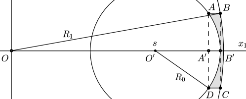
Figure 1: “Convex-concave lens” $ABCD_{\text{lens}}$ (grey) and cylinder $ABCD_{\text{cyl}}$ (dashed).

In this proof, without any ambiguity, we use $|\cdot|$ to denote the various measures such as the length, surface area and volume of the objects lie in the appropriate spaces. Let $\varepsilon>0$ be sufficiently small and let $B^{\prime}=|OB^{\prime}|\,e_{1}$ be the point such that $|OB^{\prime}|=\sqrt{R_{1}^{2}-\varepsilon^{2}}$ (see Fig. 1). Then the hyperplane perpendicular to $e_{1}$ at $B^{\prime}$ intersects with $B_{R_{1}}(0)$ by the $(N-1)$-dimensional ball $B_{1}$ of radius $|BB^{\prime}|=\varepsilon$. By choosing $s=s_{\varepsilon}=\sqrt{R_{1}^{2}-\varepsilon^{2}}-R_{0}$, we see that the ball $B_{R_{0}}(se_{1})$ touches $B_{1}$. Now consider the $N$-dimensional “convex-concave lens” $ABCD_{\text{lens}}$ bounded by the spherical caps $BC_{\text{cap}}$ and $AD_{\text{cap}}$ of the spheres $\partial B_{R_{1}}(0)$ and $\partial B_{R_{0}}(se_{1})$, respectively, and by the lateral cylindrical surface $AB_{\text{lat}}$ generated by the segment $AB$ parallel to $e_{1}$. Let $ABCD_{\text{cyl}}$ be the cylinder of radius $|BB^{\prime}|$ and height $|AB|$. For simplicity, we denote the various positive constants which are independent of $\varepsilon$ by $k.$ For $\varepsilon>0$ small enough, observe that

$$|AB| =|A^{\prime}B^{\prime}|=R_{0}-\sqrt{R_{0}^{2}-\varepsilon^{2}}\approx k\varepsilon^{2};$$

$$|AD_{\text{cap}}| >|BC_{\text{cap}}|>|B_{1}|=k\varepsilon^{N-1};$$

$$|ABCD_{\text{lens}}| <|ABCD_{\text{cyl}}|=|AB||B_{1}|\approx k\varepsilon^{2}\,\varepsilon^{N-1};$$

$$|AB_{\text{lat}}| =|AB||\partial B_{1}|\approx k\varepsilon^{2}\,\varepsilon^{N-2}.$$

Now by making use of the above estimates we obtain

$$\frac{|\partial\left(\Omega_{s}\setminus ABCD_{\text{lens}}\right)|}{|\Omega_{s}\setminus ABCD_{\text{lens}}|}=\frac{|\partial\Omega_{s}|-|AD_{\text{cap}}|-|BC_{\text{cap}}|+|AB_{\text{lat}}|}{|\Omega_{s}|-|ABCD_{\text{lens}}|}<\frac{|\partial\Omega_{s}|-2k\varepsilon^{N-1}+k\varepsilon^{N}}{|\Omega_{s}|-k\varepsilon^{N+1}}<\frac{|\partial\Omega_{s}|}{|\Omega_{s}|}$$

for sufficiently small $\varepsilon$. Therefore, there exists $s>0$ such that $h(s)<h(0).$ Now define

$$s^{*}:=\inf\{s\in[0,R_{1}-R_{0}):~{}h(0)>h(s)\}.$$ (4.3)

Since $h(s)$ is continuous, by the definition of $s^{*},$ we easily see that $h(0)=h(s^{*})$ and $h(s^{*})>h(s)$ for any $s\in(s^{*},R_{1}-R_{0})$. ∎

Remark 4.2.

Clearly $h(s)=h(0)$ for every $s\in[0,s^{*}].$ Thus, if $s^{*}>0$, then the strict monotonicity of $\lambda_{1}(s)$ fails for $p=1$. However, whether $s^{*}>0$ or not is still open. Further, the strict monotonicity of $h(s)$ on the interval $[s^{*},R_{1}-R_{0}]$ is not answered yet. It is worth to mention that a shape derivative formula for $h_{1}(\Omega)$ is obtained in [22] for $\Omega$ having just one Cheeger set. However, the uniqueness of the Cheeger set for eccentric annular regions $\Omega_{s}$ is not known.

5 Application to the Fučik spectrum

In this section we prove Theorem 1.3. For this end, we use Theorem 1.1 and the variational characterization (1.7) of $\mathscr{C}$, the first nontrivial curve of the Fučik spectrum for the eigenvalue problem (1.6), see [10]. Recall that $\mathscr{C}$ is constructed from points $(t+c(t),c(t))$, where

$$c(t)=\inf_{\gamma\in\Gamma}\max_{u\in\gamma[-1,1]}\left(\int\limits_{\Omega}|\nabla u|^{p}\,{\,\rm d}x-t\int\limits_{\Omega}(u^{+})^{p}\,{\,\rm d}x\right),\quad t\geq 0,$$

and their reflections with respect to the diagonal. See (1.8) for the definition of $\Gamma$.

Proof of Theorem 1.3: Let $\Omega$ be a bounded radial domain. Suppose there exist a point on $\mathscr{C}$ and a corresponding eigenfunction $u$ which is radial. Without loss of generality, we can suppose that $t\geq 0$ (otherwise we consider $-u$ instead of $u$). Thus $u$ satisfies the following equation:

$$\left.\begin{aligned} -\Delta_{p}u&=(t+c(t))(u^{+})^{p-1}-c(t)(u^{-})^{p-1}&&\text{in }~{}\Omega,\\ u&=0&&\text{on }~{}\partial\Omega.\end{aligned}\right\}$$

By Theorem 2.1 of [11], we know that $u$ has exactly two nodal domains, $N^{+}:=\{x\in\Omega:u(x)>0\}$ and $N^{-}:=\{x\in\Omega:u(x)<0\}.$ Since the restriction of $u$ to each of the nodal domains is an eigenfunction of $-\Delta_{p}$ with a constant sign, we easily get

$$\lambda_{1}(N^{+})=t+c(t)\text{ and }\lambda_{1}(N^{-})=c(t).$$ (5.1)

Since $u$ is radial and $\Omega$ is radially symmetric, the nodal domains are also radially symmetric. Assume for definiteness that $u$ is negative near the outer boundary of $\Omega.$ Thus there exists $R>0$ such that $N^{+}=\{x\in\Omega:|x|<R\}$ and $N^{-}=\{x\in\Omega:|x|>R\}.$ If $\Omega$ is a ball, say $B_{R_{1}}(0),$ then $N^{+}=B_{R}(0)$ and $N^{-}=A_{R_{1},R}(0,0).$ Now for $s\in(0,R_{1}-R),$ by using (5.1) and Theorem 1.1 we obtain $\lambda_{1}(B_{R}(se_{1}))=t+c(t)$ and $\lambda_{1}(A_{R_{1},R}(0,se_{1}))<c(t)$. Further, using the continuity of $\lambda_{1}(\Omega)$ (see, for instance, Theorem 1 of [13]) we can find $\widetilde{R}\in(R,R_{1})$ such that

$$\lambda_{1}(B_{\widetilde{R}}(se_{1}))<t+c(t)\text{ and }\lambda_{1}(A_{R_{1},\widetilde{R}}(0,se_{1}))<c(t).$$

If $\Omega$ is an annulus, say $A_{R_{1},R_{0}}(0,0),$ then we have $N^{+}=A_{R,R_{0}}(0,0)$ and $N^{-}=A_{R_{1},R}(0,0).$ Now for $0<s<\min\{R_{1}-R,R-R_{0}\}$ by using (5.1) and Theorem 1.1 we obtain

$$\lambda_{1}(A_{R,R_{0}}(se_{1},0))<t+c(t)\text{ and }\lambda_{1}(A_{R_{1},R}(0,se_{1}))<c(t).$$

In either case, we have two disjoint domains $\Omega_{1}$ and $\Omega_{2}$ such that

$$\lambda_{1}(\Omega_{1})<t+c(t)\text{ and }\lambda_{1}(\Omega_{2})<c(t).$$

Let $u_{1}$ and $u_{2}$ be corresponding eigenfunctions. Clearly $u_{1}$ and $u_{2}$ have disjoint supports and

$$\int\limits_{\Omega}|\nabla u_{1}|^{p}{\,\rm d}x<(t+c(t))\int\limits_{\Omega}|u_{1}|^{p}{\,\rm d}x\text{ and }\int\limits_{\Omega}|\nabla u_{2}|^{p}{\,\rm d}x<c(t)\int\limits_{\Omega}|u_{2}|^{p}{\,\rm d}x.$$

The above inequalities lead to a contradiction to the definition (1.7) of $c(t)$ by the same arguments as in the proof of Theorem 3.1 of [10]. Thus $u$ must be nonradial. This completes the proof. ∎

T. V. Anoop: Department of Mathematics, Indian Institute of Technology Madras, Chennai 36, India.
Email: anoop@iitm.ac.in

Vladimir Bobkov: Department of Mathematics and NTIS, Faculty of Applied Sciences, University of West Bohemia, Univerzitní 8, Plzeň 306 14, Czech Republic.
Institute of Mathematics, Ufa Scientific Center, Russian Academy of Sciences, Chernyshevsky str. 112, Ufa 450008, Russia.
Email: bobkov@kma.zcu.cz

Sarath Sasi: School of Mathematical Sciences, National Institute for Science Education and Research Bhubaneswar, Jatni 752050, India.
Email: sarath@niser.ac.in

References

- [1] T. V. Anoop, P. Drábek, and S. Sasi. On the structure of the second eigenfunctions of the -Laplacian on a ball. Proceedings of the American Mathematical Society, 144(6):2503–2512, 2016.
- [2] M. S. Ashbaugh and R. D. Benguria. Isoperimetric inequalities for eigenvalues of the Laplacian. In Proceedings of Symposia in Pure Mathematics, volume 76, pages 105–139. Providence, RI; American Mathematical Society; 1998, 2007.
- [3] G. Barles. Remarks on uniqueness results of the first eigenvalue of the -Laplacian. Toulouse. Faculté des Sciences. Annales. Mathématiques. Série 5, 9(1):65–75, 1988.
- [4] T. Bartsch and M. Degiovanni. Nodal solutions of nonlinear elliptic Dirichlet problems on radial domains. Atti della Accademia Nazionale dei Lincei. Classe di Scienze Fisiche, Matematiche e Naturali. Rendiconti Lincei. Serie IX. Matematica e Applicazioni, 17(1):69–85, 2006.
- [5] T. Bartsch, T. Weth, and M. Willem. Partial symmetry of least energy nodal solutions to some variational problems. Journal d’Analyse Mathématique, 96:1–18, 2005.
- [6] J. Benedikt, P. Drábek, and P. Girg. The first nontrivial curve in the Fučik spectrum of the Dirichlet Laplacian on the ball consists of nonradial eigenvalues. Boundary Value Problems, 2011(1):1–9, 2011.
- [7] H. Bueno and G. Ercole. On the -torsion functions of an annulus. Asymptotic Analysis, 92(3-4):235–247, 2015.
- [8] A. M. H. Chorwadwala and R. Mahadevan. An eigenvalue optimization problem for the -Laplacian. Proceedings of the Royal Society of Edinburgh: Section A Mathematics, 145(6):1145–1151, 2015.
- [9] A. M. H. Chorwadwala, R. Mahadevan, and F. Toledo. On the Faber–Krahn inequality for the Dirichlet -Laplacian. ESAIM: Control, Optimisation and Calculus of Variations, 21(1):60–72, 2015.
- [10] M. Cuesta, D. de Figueiredo, and J.-P. Gossez. The beginning of the Fučik spectrum for the -Laplacian. Journal of Differential Equations, 159(1):212–238, 1999.
- [11] M. Cuesta, D. G. De Figueiredo, and J.-P. Gossez. A nodal domain property for the -Laplacian. Comptes Rendus de l’Académie des Sciences. Série I. Mathématique, 330(8):669–673, 2000.
- [12] P. R. Garabedian and M. Schiffer. Convexity of domain functionals. Journal d’Analyse Mathématique, 2(2):281–368, 1952.
- [13] J. García Melián and J. Sabina de Lis. On the perturbation of eigenvalues for the -Laplacian. Comptes Rendus de l’Académie des Sciences. Série I. Mathématique, 332(10):893–898, 2001.
- [14] E. M. Harrel II, P. Kröger, and K. Kurata. On the placement of an obstacle or a well so as to optimize the fundamental eigenvalue. SIAM Journal on Mathematical Analysis, 33(1):240–259, 2001.
- [15] A. Henrot. Extremum problems for eigenvalues of elliptic operators. Springer Science & Business Media, 2006.
- [16] J. Hersch. The method of interior parallels applied to polygonal or multiply connected membranes. Pacific Journal of Mathematics, 13(4):1229–1238, 1963.
- [17] P. Juutinen, P. Lindqvist, and J. J. Manfredi. The -eigenvalue problem. Archive for rational mechanics and analysis, 148(2):89–105, 1999.
- [18] B. Kawohl and V. Fridman. Isoperimetric estimates for the first eigenvalue of the -Laplace operator and the Cheeger constant. Commentationes Mathematicae Universitatis Carolinae, 44(4):659–667, 2003.
- [19] S. Kesavan. On two functionals connected to the Laplacian in a class of doubly connected domains. Proceedings of the Royal Society of Edinburgh. Section A. Mathematics, 133(3):617–624, 2003.
- [20] J. C. Navarro, J. D. Rossi, A. San Antolin, and N. Saintier. The dependence of the first eigenvalue of the infinity Laplacian with respect to the domain. Glasgow Mathematical Journal, 56(02):241–249, 2014.
- [21] A. Nazarov. The one-dimensional character of an extremum point of the Friedrichs inequality in spherical and plane layers. Journal of Mathematical Sciences, 102(5):4473–4486, 2000.
- [22] E. Parini and N. Saintier. Shape derivative of the Cheeger constant. ESAIM: Control, Optimisation and Calculus of Variations, 21(2):348–358, 2015.
- [23] A. G. Ramm and P. N. Shivakumar. Inequalities for the minimal eigenvalue of the Laplacian in an annulus. Mathematical Inequalities & Applications, (4):559–563, 1998. Updated version: arXiv:math-ph/9911040.
- [24] J. Sokolowski and J.-P. Zolésio. Introduction to shape optimization, Shape sensitivity analysis, volume 16 of Springer Series in Computational Mathematics. Springer-Verlag, Berlin, 1992.
- [25] J. L. Vázquez. A strong maximum principle for some quasilinear elliptic equations. Applied Mathematics and Optimization, 12(1):191–202, 1984.