SPECTRA AND BIFURCATIONS

Abstract

The concept of spectrum for a class of non-linear wave equations is studied. Instead of looking for stability, the key to the spectral structure is found in the instability phenomena (bifurcations). This aspect is best seen in the ‘classical model’ of the non-linear wave mechanics. The solitons (macro-localizations) are a part of the non-linear spectral problem; their bifurcations reflect the dynamical symmetry breaking. The computer simulations suggest that the bifurcations of the asymptotic behaviour occur also for the general, non-stationary states. A phenomenon of the soliton splitting is observed.

^aInterdisciplinary Centre for Mathematical and Computational Modelling,
Warsaw University,
Pawińskiego 5a, 02-106 Warsaw, Poland.
^bDepartment of Biophysics, Warsaw University,
Żwirki i Wigury 93, 02-089 Warsaw, Poland.
^cDepartamento de Fisica, CINVESTAV,
A.P. 14-740, 07000 México DF, México.

1 Introduction

In the last decades one can observe a renewed interest in non-linear wave equations [1, 2, 3, 4, 5, 6, 7, 8, 9, 10, 11]. The simplest class of non-linear Schrödinger’s equations creates a temptation to formulate a “quantum mechanics” with $\psi\in L^{2}(R^{3})$, $|\psi|^{2}$ as the probability density [3, 6, 12] but with the superposition principle broken. In turn, the non-linear Schrödinger’s equation with an atypical kinetic energy [12, 13]:

$$i\frac{\partial\psi}{\partial t}=-\frac{1}{2}\Delta(|\psi|^{\alpha}\psi)+V({\bf x},t)\psi$$ (1.1)

$(\alpha\in R)$, has the absolutely conservative integral:

$$N[\psi]=\int_{R^{3}}|\psi|^{2+2\alpha}d_{3}x={\rm const}$$ (1.2)

suggesting a statistical theory with $\psi\in L^{p}(R^{3}),\;p=2+2\alpha$ and with $|\psi|^{p}$ defining the probability density. A slightly different equation:

$$i\frac{\partial\psi}{\partial t}=-\frac{1}{2}|\psi|^{-\alpha}\Delta(|\psi|^{\alpha}\psi)+V({\bf x},t)\psi$$ (1.3)

admits the conservative integral:

$$N[\psi]=\int_{R^{3}}|\psi|^{2+4\alpha}d_{3}x={\rm const}$$ (1.4)

asking for the space of states $L^{k}(R^{3})$ $(k=2+4\alpha$). Curiously, (1.3) has the same spectrum as the conventional Schrödinger equation (a counterexample against the belief that the non-linearity can be tested by observing the spectral frequencies). The eqs. (1.1-3) are not Galileo covariant; however, cases of Galileo invariant wave mechanics were recently found by Doebner and Goldin [7, 8]; see also Dodonov and Mizrahi [9], and Natterman [14]. One of hopes in the non-linear schemes is that they might help to understand the collapse of the wave packets (see e.g. Gisin [15]), but one of obstacles is that the non-linearity could generate faster than light signals in a non-linear analogue of EPR arrangements (a disquieting observation of Gisin [16] and Czachor [5] leaves the ‘fundamental non-linearity’ in defense, but not in defeat!).

Apart of fundamental reasons, the non-linear wave eqs. might be of practical interest, as tools to describe dense clouds of interacting quanta. To this subject belong all variants of ‘self-consistent’ wave mechanics [17, 18], the theories which model the feedback interactions of a micro-object with a mezoscopic or macroscopic medium, in molecular [19, 20] or solid state physics [10, 11]. In all these schemes, the ‘localizations’ (bound states) bring a relevant information. However, some structural problems are still open.

One of unsolved questions in non-linear theories is the problem of spectrum. Is it pertinent to define spectra for non-linear operators [21, 3, 6]? Looking for similarities between the linear and non-linear cases, one might be tempted by the idea of stability. In fact, in the orthodox quantum theory the bound states are stationary and stable; in non-linear case the same concerns solitons; a lot of authors marvel about the soliton ability to survive collisions! Yet, the story has its opposite side, which seems to be as relevant for the non-linear spectral problem.

One of curious aspects of the Schrödinger’s eigenvalue equation in 1-space dimension is the possibility of reinterpreting the space coordinate $x$ as the “time” ($x=t$), the wave function $\psi$ as the coordinate and the derivative $\psi^{\prime}$ as the momentum of a certain classical point particle [22, 23, 24, 25, 26, 27]. What one obtains is a classical model for quantum phenomena or vice versa [24, 28, 29] (see, e.g., the interpretation of the Saturn rings as spectral bands [30]). It turns out that the ‘classical image’ throws also some new light onto the non-linear spectral problem. It shows that the eigenstates correspond to bifurcations [21, 31, 32, 33, 34, 35]; in a sense, they are “born of instability”!

Our paper is precisely dedicated to the instability (bifurcation) aspects of the one dimensional spectral problem. We shall show that they provide the most natural bridge between the linear and non-linear cases, leading also to the easiest numerical algorithm to determine the spectral values. Among many models which can be used to illustrate this, we have selected the simplest one, with some hope that observations presented below might turn generally useful.

2 The ‘classical portrait’.

We shall consider the non-linear Schrödinger’s equation in 1-space dimension:

$$i\frac{d}{dt}\Psi(x,t)=-\frac{1}{2}\frac{d^{2}\Psi}{dx^{2}}+V(x)\Psi+\varepsilon f(|\Psi|^{2})\Psi$$ (2.1)

where $V(x)$ is an external potential and $f()$ a given function defining the non-linearity. The stationary solutions $\Psi(x,t)$ = exp $(-iEt)\psi(x)$ then fulfill:

$$-\frac{1}{2}\frac{d^{2}\psi}{dx^{2}}+[V(x)-E]\psi+\varepsilon f(|\psi|^{2})\psi=0$$ (2.2)

The simple harted analogue of an eigenstate can be introduced without difficulty [21, 31, 32, 33, 34, 35]. Whenever $\psi$ in (2.2) is localized, i.e. vanishes for $x\rightarrow\pm\infty$, then $\psi$ will be called a ‘localized state’ and $E$ will be interpreted as a discrete frequency eigenvalue of (2.2). We use the traditional symbol $E$ but we speak about the frequency instead of energy eigenvalue to remind that for the non-linear Schrödinger’s equation (2.2) the parameter $E$ may have no energy interpretation (this point is widely discussed in [3, 6]).

Denoting now $x=t$, $\psi=q_{1}+iq_{2}$, $\psi^{\prime}=p_{1}+ip_{2}$ one immediately reduces (2.2) to the Newton’s equation of motion:

$$\frac{d{\bf q}}{dt}={\bf p},~{}~{}~{}\frac{d{\bf p}}{dt}=2[V(t)-E]{\bf q}+2\varepsilon f({\bf q}^{2}){\bf q}.$$ (2.3)

for a classical point particle in a radial, centrally symmetric force field in 2 space dimensions, where ${\bf q,p}$ denote the two-component position and momentum vectors. The Hamiltonian is:

$$H(t)={\bf p}^{2}/2+[E-V(t)]{\bf q}^{2}-\varepsilon F({\bf q}^{2}),$$ (2.4)

with $F(\zeta)=\int f(\zeta)d\zeta$. For every $E\in R$ the eq.(2.3), of course, has a family of solutions labelled by 2 complex (or 4 real) parameters, but very seldom it has solutions vanishing for both $t\rightarrow+\infty$ and $t\rightarrow-\infty$. More seldom even they will vanish quickly enough to assure:

$$\int_{-\infty}^{+\infty}|\psi(x)|^{2}dx=\int_{-\infty}^{+\infty}{\bf q}(t)^{2}dt<+\infty$$ (2.5)

Whenever (2.3) admits non-trivial solutions vanishing at $t\rightarrow\pm\infty$, $E$ is an eigenvalue (proper frequency) of (2.2). We adopted again the traditional concept of the spectrum in the non-linear case, [21, 31, 32, 33, 34, 35], to be further discussed in our section 5.

3 Classical orbits and bound states

One of advantages of the ‘classical picture’ is that it permits to exploit experiences of classical mechanics to describe the ‘bound states’ (2.3) and one of the most obvious ideas is to use the classical motion integrals. As the force field in (2.3-4) is radial and centrally symmetric, the angular momentum of each trajectory is constant. Introducing the polar variables $q_{1}$ = $r\cos\alpha$, $q_{2}$ = $r\sin\alpha$, one has:

$$M={q_{1}}{p_{2}}-{q_{2}}{p_{1}}=r^{2}\dot{\alpha}=\text{const}.$$ (3.1)

The canonical eqs. (2.3) now imply:

$$\frac{d^{2}r}{dt^{2}}=2[V(t)-E]r+2\varepsilon f(r^{2})r+M^{2}/r^{3}$$ (3.2)

interpretable as Newton eq. of motion in 1 space dimension. If $M\not=0$, the last term prevents $r$ (and ${\bf q}$) from tending to zero:

Proposition 1.

If $V(t)$ is limited from below and $M\not=0$ then the solution $r(t)$ of (3.2) cannot tend to zero neither for a finite $t$ nor for $t\rightarrow\pm\infty$.

Proof.

Indeed, for a non-trivial trajectory ($r(t)\not\equiv 0$) two first terms on the right side of (3.2) create either repulsive or limited attractive forces and cannot counterbalance the third term $M^{2}/r^{3}$ which prevents the material point from approaching too close to zero. ∎

As a consequence, for $M\neq 0$ the integral (2.5) diverges for any $E\in R$. Thus, the non-trivial localized solutions of (2.3), (with $q\not\equiv 0$) if they exist, must fulfill $M$=$0$ $\Rightarrow\dot{\alpha}$=$0$ $\Rightarrow$ $\alpha$=$const$. Without loosing generality, all bound states of (2.2) can be therefore obtained for $\alpha\equiv 0$, i.e., for $\psi$ real. In terms of the trajectory interpretation (2.3) it means that the bound states can be determined just by solving the 1-dimensional (instead of the 2-dimensional) motion problem with:

$$H(q,p,t)=p^{2}/2+[E-V(t)]q^{2}-\varepsilon F(q^{2}),~{}~{}~{}q,p\in R$$ (3.3)

and

$$\frac{dq}{dt}=p,~{}~{}~{}\frac{dp}{dt}=2[V(t)-E]q+2\varepsilon f(q^{2})q.$$ (3.4)

4 Spectra as bifurcations.

While values of $E$ which permit trajectories (3.4) vanishing on both ends $t\rightarrow\pm\infty$ are exceptions, yet for any $E$ eq. (3.4) typically admits a subclass of solutions vanishing for $t\rightarrow-\infty$ (the ‘left vanishing cues’), as well as another subclass vanishing for $t\rightarrow+\infty$ (the ‘right vanishing cues’). Indeed:

Proposition 2.

Suppose $f(\zeta)$ is continuous in $[0,+\infty)$ with $f(0)=0$, while $V(t)$ is defined and continuous outside of a finite interval $[a,b]$ with two (proper or improper) limits:

$$V_{1}=\lim_{t\rightarrow-\infty}V(t)>-\infty,~{}~{}~{}V_{2}=\lim_{t\rightarrow+\infty}V(t)>-\infty$$ (4.1)

Then for any $E<V_{2}$, $t_{o}>b$, there is $K_{2}>0$ such that for any $q_{o}\in R$, $|q_{o}|\leq K_{2}$ the Hamiltonian (3.3) admits at least one trajectory $q(t)$ with $q(t_{o})$ = $q_{o}$ and $q(t)\rightarrow 0$ for $t\rightarrow+\infty$. Similarly, for any $E<V_{1}$, $t_{o}<a$, there is $K_{1}>0$ such that for any $q_{o}\in R$, $|q_{o}|<K_{1}$, there is at least one integral trajectory $q(t)$ with $q(t)\rightarrow 0$ for $t\rightarrow-\infty$.

(Proof is an exercise in shooting [26, 27]. Note: the conclusion of the theorem holds also for some non-linear eqs. with $f(\zeta)$ singular at $\zeta$=0 [3]).

To illustrate the structure of the cues we shall consider the case of a finite potential well with $V(t)\leq 0$ and $V(t)\equiv 0$ outside of a finite interval $[a,b]$. The trajectory q(t) outside of [a,b] then corresponds to the motion of a classical point in a static potential, with the Hamiltonian:

$$H(t)=H_{o}=p^{2}/2+Eq^{2}-\varepsilon F(q^{2}),~{}~{}~{}t\not\in[a,b]$$ (4.2)

The solutions asymptotically vanishing at $t\rightarrow\pm\infty$ are the orbits for which the Hamiltonian (4.2) vanishes, i.e:

$$p=\pm q\sqrt{2}\sqrt{-E+\varepsilon F(q^{2})/q^{2}}=\pm\eta(q,E)$$ (4.3)

the signs + (or - ) label the solutions vanishing at $t\rightarrow-\infty$ ($t\rightarrow+\infty$), respectively. If one forgets about the exact t-dependence, the condition (4.3) determines just two evolution-invariant curves (a part of the ‘phase portrait’ of (2.2), cf.[36]):

$$I_{\pm}(E)=\{(q,p):p=\pm\eta(q,E)\}.$$ (4.4)

Under the exclusive influence of the free Hamiltonian (4.2) (i.e., for $V(t)\equiv 0$), the canonical evolution produces a ‘curvilinear squeezing’ which distinguishes the $I_{\pm}(E)$ lines: $I_{+}(E)$ expands (the points on $I_{+}(E)$ escape from the phase space origin as $t$ increases from $t$=$-\infty$), whereas $I_{-}(E)$ shrinks (the points of $I_{-}(E)$ tend to the origin as $t\rightarrow+\infty$). If one solves (4.3) including the exact time dependence:

$$\dot{q}=\pm\eta(q,E).$$ (4.5)

then the points on $I_{+}(E)$ originate the left vanishing cues (i.e. the solutions of (2.2-3) vanishing at $t\rightarrow-\infty$), whereas the points of $I_{-}(E)$, the right vanishing cues (tending to zero as $t\rightarrow+\infty$). If $I_{+}(E)$ and $I_{-}(E)$ don’t connect outside of the origin, the solutions in the form of bound states can arise only due to the potential $V(t)\not\equiv 0$. The number $E$ is an eigenvalue of (2.2) if the evolution enforced by $V(t)$ in the interval $[a,b]$ transforms one of the left-vanishing cues into one of the right-vanishing cues (thus drawing a wave function which vanishes on the both ends $t\rightarrow\pm\infty$; compare [27]). The effect has rather little to do with the linearity. The linearity is a marginal property of the orthodox Schrödinger’s dynamics - whereas the existence of the ‘bound states’ is the topological phenomenon, caused by an abrupt change (bifurcation) which produces the homoclinic orbits of (3.4) (compare Guckenheimer and Holmes [36]). The mechanism of this effect can be easily monitored.

Suppose, we keep $E$ fixed but change $V(t)$ putting $V(t)=\lambda\phi(t)$, with $\phi$ fixed and $\lambda>0$ variable. Observe then a congruence of orbits sticking at $t=a$ from a given point of $I_{+}(E)$. If $\lambda=0$, then the orbit sticks to $I_{+}(E)$ forever. Assume now, we switch on slowly the potential term $V(t)=\lambda\phi(t)$. For small $\lambda>0$ the motion is slightly modified (the trajectory is pushed out of $I_{+}(E)$) though it returns to $I_{+}(E)$ asymptotically as $V(t)$ disappears. When $\lambda$ increases, the type of the motion changes. In the time interval where $V(t)-E=\lambda\phi(t)-E<0$ the Hamiltonian (3.3) becomes an attractive anharmonic oscillator and causes a circulation around the origin instead of squeezing. Everytime the circulating point $(q(b),p(b))$ crosses the line $I_{-}(E)$, the asymptotic behaviour of the trajectory suddenly changes. At the exact bifurcation value of $\lambda$ the point $(q(b),p(b))$ ends up on $I_{-}(E)$; henceforth, for $t>b$, the potential-free motion (4.2) returns $(q(t),p(t))$ to zero drawing an exceptional, closed orbit (a bound state of $\lambda\phi(t)$ for the eigenvalue $E$). An analogous picture arises for $V(t)$ fixed but $E$ changing. To illustrate the phenomenon, we have applied the computer simulation to obtain a family of canonical trajectories of (3.3) for a fixed $E<0$ and the potential well $\phi(t)$ given by the forthcoming formula (8.1). The bifurcations lead to the bound states illustrated on Fig. 1.

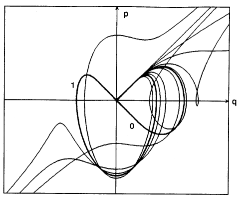
Figure 1: A congruence of classical trajectories of (3-5) in process of bifurcation. $V(\cdot)$ given by (8.1). The bold lines 0, 1 mark two lowest bound orbits created at the bifurcation values of $\lambda$ [27]. An analogues phenomenon can be seen for $\lambda$ fixed and $E$ varying.

Note, that we have arrived at a certain general scheme for generating the bound states, which no longer requires linear spaces and linear operators. A similar phenomenon would occur on any 2-dim. symplectic manifold ${\cal P}$ (compare Klauder [37]), with two flows generated by two ‘antagonistic’ vector fields A and B sharing a common fixpoint 0.

The flow A should be a squeezing, with a saddle point at 0 and with the phase portrait dominated by two intersecting invariant lines: $I_{+}$ expanding, $I_{-}$ shrinking (see Fig. 2). The field B, in turn, should be a circulation, with orbits in form of closed loops surrounding the fixpoint 0 (compare Guckenhaimer and Holmes [36, p.52, Fig. 1.8.6]).

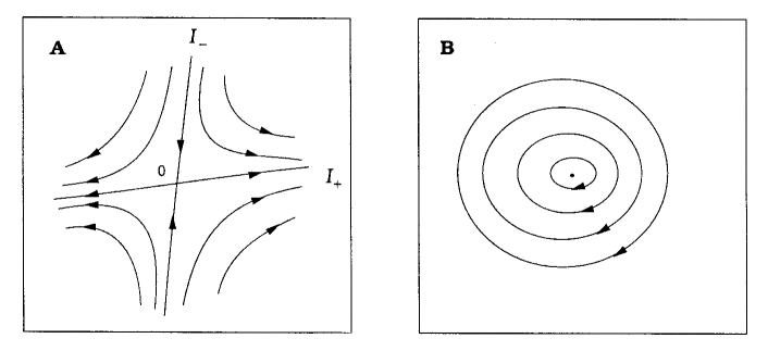
Figure 2: The imitation of the spectral phenomenon by two vector fields, ${\bf A}$ and ${\bf B}$, with coinciding fixpoints of different types on an arbitrary 2-dim surface. The bifurcations of the orbit driven by ${\bf A}+\lambda\phi(t){\bf B}$ occur whenever the circulation generated by ${\bf B}$ changes the assymptotic form of the trajectory allowed by ${\bf A}$ (compare Guckenheimer and Holms [36, p. 52].

If now the phase point ${\bf q}(t)\in$ ${\cal P}$ moves under the influence of a combined vector field ${\bf A}+\lambda\phi(t){\bf B}$ (where $\lambda\geq 0$ is a variable amplitude and $\phi(t)\geq 0$), then, as $\lambda$ increases, the number of intersections of the phase trajectory with the shrinking line $I_{-}$ grows too. At each new intersection, the trajectory bifurcates, forming an exceptional, closed orbit, interpretable as a bound state.

Our example is oversimplified - but it shows that the mechanism of creation of the bound states (at least in the 1-dimensional case) is not metrical but par excellence topological. If the theory is non-linear, the orthogonality of the bound states desappears - but the bifurcation mechanism still works, distinguishing the spectral parameters for the non-linear system. Notice, that the idea of spectrum as a sequence of bifurcations has already emerged in some mathematical areas, e.g. in studies of chaotic systems [38, 39]. It is still an open problem whether the similar idea could work in higher dimensions or for the abstract non-linear operators. We shall see, however, that as far as 1-space dimension is considered, it leads to some efficient numerical techniques.

5 Numerical algorithm and Zakharov well.

To determine numerically the bifurcation spectra, we propose a simple variant of the shooting method involving only the integration in a finite interval. To illustrate it let’s consider again eq. (2.2) with $V(t)$ forming a limited potential well ($V(t)\equiv 0$ for $t\not\in[a,b]$). For any $E\in R$ we then choose an initial point ${\bf q}(a)$ in $I_{+}(E)$ and integrate (2.3) in $[a,b]$ finding the ‘final point’ ${\bf q}(b)=(q(b),p(b))$.

Whenever for an ‘initial point’ ${\bf q}(a)=(q_{a},p_{a})\in I_{+}(E)$ the ‘final point’ ${\bf q}(b)$ happens to be on $I_{-}(E)$, the shooting exercise was a success: the number E is then an eigenvalue of (2.2) and the orbit of (2.3) [defined by the initial condition ${\bf q}(a)=(q_{a},\eta(q_{a},E))$] represents a bound state of (2.2). The set of data $(q_{a},E)$ for which this happens, typically, forms a sequence of lines on the $(q_{a},E)$ diagramme. The different branches $E_{n}=E_{n}(q_{a})$ correspond to the different numbers of times the phase trajectory crosses the shrinking line $I_{-}(E)$ for $t\in(a,b)$ (see Fig. 1). The non-trivial $q_{a}$-dependence of the branches $E_{n}$ reflects the fact that for the non-linear eq. (2.2) the eigenvalues, in general, depend on the norm.

The existence of the localized states (solutions vanishing at $t\rightarrow\pm\infty$) does not yet assure that they must be square integrable. In fact, for the eq. (2.2) the cues are determined by the structural function $F(\zeta)$; their square integrability depends on the convergence of the integrals:

$$\int\frac{\dot{q}qdt}{\sqrt{-E+\varepsilon F(q^{2})/q^{2}}}=\int\frac{d\zeta}{\sqrt{-E+\varepsilon F(\zeta)/\zeta}}$$ (5.1)

around $\zeta=q^{2}=0$. Presumably, there might be non-linear theories with localized solutions vanishing so slowly at $t\rightarrow\pm\infty$ that the integrals (5.1) diverge. The physical sense of such localizations is an open problem. Below, we shall consider non-linearities for which this does not occur. If this is the case, each (non-trivial) bound state possesses a finite norm (2.5) which apports an essential physical information (in contrast to the linear theory, where the norm is arbitrary). The information about the norm, however, is difficult for the computer manipulations: (2.5) is finite only for exceptional trajectories (bound states); for all other solutions is infinite. To facilitate numerical operations we thus introduced the pseudo-norm, well defined, continuous, for all solutions, and coinciding with (2.5) whenever the solution is localized.

Definition.

For any integral trajectory $q(t)$, the pseudonorm $N(q)$ is:

$$N(q)=\int_{-\infty}^{a}q_{+}(t,E)^{2}dt+\int_{a}^{b}q(t)^{2}dt+\int_{b}^{+\infty}q_{-}(t,E)^{2}dt\\ =N_{+}(q)+N_{o}(q)+N_{-}(q)$$ (5.2)

where $q_{\pm}(t,E)$ are two ‘vanishing cues’, defined in $(-\infty,a]$ and $[b,+\infty)$, joining $q(t)$ at $t=a$ and $t=b$ respectively (i.e., $q_{+}(a,E)=q(a)$; $q_{-}(b,E)=q(b)$, without demanding the continuity of the derivatives).

From the definition, (5.2) is always finite; moreover, if $q(t)$ is a bound state, then $q_{\pm}(t,E)=q(t)$ and the pseudonorm (5.2) reduces to the true norm (2.5). Each isonorm line $N$=const, typically, crosses the eigenvalue lines $E=E_{n}(q_{a})$ ($n$=0,1,…); the intersections determine the eigenvalues for the bound states of the same norm $N$. In particular, the line $N$=1 defines the ‘traditional’ sequence of eigenvalues $E_{n}$ ($n$=0,1,…) for all bound states of norm 1.

To check the method, we have found the ‘localizations’ for the eq. of Zakharov type [40]:

$$-\frac{1}{2}\frac{d^{2}\psi}{dx^{2}}+[V(x)-E]\psi+\varepsilon|\psi|^{2}\psi=0$$ (5.3)

in presence of the rectangular potential well symmetric with respect to $t=0$:

$$V(t)\left\{\begin{array}[]{ll}=V_{o}&\mbox{for $t\in[-b,b]$}\\ \equiv 0&\mbox{for $t\not\in[-b,b]$}\end{array}\right.,~{}~{}~{}V_{o}<0.$$ (5.4)

Here, $a=-b$, $f(\zeta)=\zeta$, $F(\zeta)=\zeta^{2}/2$, and the expanding/shrinking curves $I_{\pm}(E)$ are given by:

$$p(q)=\pm\sqrt{\varepsilon q^{4}-2Eq^{2}}.$$ (5.5)

To find the norms, it helps that the bound states are of definite parity inside of $[-b,b]$. In fact, since $H_{o}=p^{2}/2+[E-V_{o}]q^{2}-\varepsilon q^{4}/2$ is a conserved quantity in $[-b,b]$, one has $q(b)=\pm q(-b)=\pm q_{a}$ for any bound state. Moreover, the Zakharov eq. (5.3) belongs to the list of cases where the integrals (5.1-2) are explicitly known:

$$N_{\pm}=\frac{2}{\varepsilon\sqrt{2}}\left(\gamma\sqrt{|E|+\varepsilon q_{a}^{2}/2}-\sqrt{|E|}\right),$$ (5.6)

where $\gamma=+1$ for the short cues and $\gamma=-1$ for the long cues (the last case possible only for $\varepsilon<0$). The numerical calculus intervenes only in the finite interval $[-b,b]$. We have applied the Runge-Kutta method integrating the canonical eqs. (2.3) in $[-b,b]$ for the set of the initial points ${\bf q}_{a}=(q_{a},\eta(q_{a},E))\in I_{+}(E)$. For each such ${\bf q}_{a}$ we have determined the sequence of values $E=E_{n}$ for which the ‘end points’ reach $I_{-}(E_{n})$. Differently than in the linear theory, the whole ladder depends on the initial value $q_{a}$ giving rise to the sequence of functions $E=E_{n}(q_{a})$ as shown on our Fig. 3. Their intersections with the isonorm lines determine the eigenvalues for each given norm.

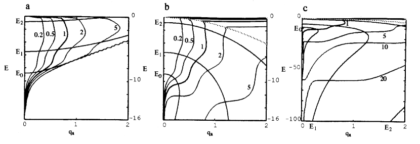
Figure 3: Three maps of the norm dependent $E$-values for the Zakharov packets in the square potential well with the bottom at $V_{o}$ = -10 and $b=1.6$. The fat lines represent the packet with the norm 1. The eigenvalues for packets of any given norm are determined by the intersections of the $E_{n}$-lines with the corresponding norm line. (a) $\varepsilon>0$ (the self-repulsive packets) the eigenvalues are above the orthodox ones; (b-c) $\varepsilon<0$ (self-attractive packets) the ground state admits $E_{o}$ below the bottom of the well (e.g. $E_{o}\approx-10.4$ for the packet norm 1, $E_{o}\approx-12.2$ for the packet norm 2). The gray lines fence off top-right regions of the diagrammes where the pseudonorm is indetermined.

As can be observed, the eigenvalues for the states of small norms (‘little eigenstates’) are almost the same as in the linear theory. The best conceptual analogy with the orthodox (linear) wave mechanics is achieved on the isonorm line $N=1$ ( $|q(t)|^{2}$ interpretable simply as the probability density). For the ‘wave packets’ of norms $>1$ the statistical interpretation is no longer obvious; more appealing would be to interpret them as localized ‘drops of quantum matter’ obeying the non-linear eq. (2.1-2) due to the internal interactions (compare [10, 11]). Indeed, such an idea is recently adopted in works dedicated to boson condensations [41, 42, 43, 44]. Observe that for the bound states of high norm the lowest eigenvalue can be much below the bottom of the well (Fig. 3c); a phenomenon unknown in the linear theory, of tentative interest in physics of the condensed mater [41, 42, 43, 44, 45].

It might be interesting to notice that our algorithm works also for the non-linear model recently proposed by Diez et al. [10, 11] permitting to determine the bound states in case of a double barrier. For $V(t)\equiv 0$ the asymptotic cues are exactly as in the linear theory.

6 The Zakharov localizations in a $\delta$-well.

An extremally simple solution of the spectral problem (5.3) is obtained for $V(t)$ in form of a $\delta$-well: $V(t)=-\Omega\delta(t)$, $\Omega>0$. The non-linear equation (2.2) for $E<0$ traduces itself into a canonical motion problem for a classical point moving under the influence of a constant potential $Eq^{2}-\varepsilon F(q^{2})$ , corrected at $t=0$ by a sudden attractive shock. The time-dependent classical Hamiltonian reads:

$$H(t)=p^{2}/2+[E+\Omega\delta(t)]q^{2}-\varepsilon F(q^{2})$$ (6.1)

The trajectory ${\bf q}(t)=(q(t),p(t))$ which vanishes at both extremes $t\rightarrow\pm\infty$ is composed exclusively of two vanishing cues, with the $p$-jump at $t=0$ caused by the $\delta$-pulse of an attractive force. Denote $q_{o}=q(0_{-})=q(0_{+})$ and $p_{o}=p(0_{-})$. The expression (4.3) then requires $p(0_{+})=-p_{o}$. On the other hand, the momentum jump is produced by the pulse of force:

$$\Delta p=p(0_{+})-p(0_{-})=-2p_{o}=\int_{0_{-}}^{0_{+}}{\cal F}(t)dt=-2\Omega\int_{0_{-}}^{0_{+}}q(t)\delta(t)dt=-2\Omega q_{o}$$ (6.2)

Taking $p_{o}$ from eq. (4.3) one has:

$$p_{o}=q_{o}\sqrt{2}\sqrt{-E+\varepsilon F(q_{o}^{2})/q_{o}^{2}}=\Omega q_{o}$$ (6.3)

and so:

$$E=-\Omega^{2}/2+\varepsilon F(q_{o}^{2})/q_{o}^{2}$$ (6.4)

i.e., the standard eigenvalue $-\Omega^{2}/2$ is corrected by the non-linear term. Assuming that $F\geq 0$ in vicinity of zero, one sees again that for $\varepsilon<0$ (the self-attractive packets) the creation of a localized states is possible for a lower $E$, whereas for $\varepsilon>0$ (self-repulsion) the non-linearity prevents to trap the packet (the bound state occurs on a higher $E$ level).

In particular, for the Zakharov eq. (5.3):

$$E=-\Omega^{2}/2+\varepsilon q_{o}^{2}/2$$ (6.5)

the norm integral (5.1) is elementary:

$$N(\psi)=\int_{-\infty}^{+\infty}q(t)^{2}dt=\frac{1}{\sqrt{2}}\int_{o}^{q_{0}^{2}}\frac{d\zeta}{\sqrt{-E+\varepsilon\zeta/2}}=\frac{4}{\varepsilon\sqrt{2}}[\sqrt{-E+\varepsilon q_{o}^{2}/2}-\sqrt{-E}]$$ (6.6)

Determining $q_{o}^{2}$ from (6.5),

$$q_{o}^{2}=(2E+\Omega^{2})/\varepsilon$$ (6.7)

and substituting into (6.6) with $N=1$ one obtains,

$$\sqrt{-2E}=\Omega-\varepsilon/2$$ (6.8)

Since $\sqrt{-2E}$, from definition, is non-negative, the solution exists only if $\varepsilon\leq 2\Omega$ (too strong non-linearity prevents the localizations! Compare with an approximate result in the theory of Bose condensation [43]). One henceforth obtains:

$$E=-(1/2)(\Omega-\varepsilon/2)^{2}$$ (6.9)

Note also, that if $\Omega<0$, $\varepsilon\leq 4\Omega$ (the case of delta barrier and self attractive packet) the long cues of Zakharov packet make possible the construction of a huge localized state with the eigenvalue given by the identical formula (6.9).

7 Macrostates

For a class of non-linear eqs. the ‘bound states’ exist even in absence of potential. The phenomenon depends obviously on the global structure of the squeezing group. It occurs whenever for some $E$ the 1-dim manifold $H=0$ is a closed loop (the expanding and shrinking lines $I_{\pm}(E)$ connect). If this is the case, the time dependent point moving along the loop $I_{\pm}(E)$ paints a huge localized state $\psi$. The norm of $\psi$ cannot be arbitrarily small (it is exactly determined by the value of E and by the nonlinearity); we thus call $\psi$ a macro-state or macro-localization. The links with solitons are immanent. The ‘solitonology’ usually describes ‘traveling waves’ $\Psi(x,t)$, with the stability aspects stressed and spectral aspects forgotten. However, for the Galileo invariant theory both phenomena are the same: the ‘traveling waves’ are just Galileo transformed macrostates. This would suggest that the solitons too must share the bifurcation aspects of the bound states! We shall show that this indeed occurs. Let us return to the non-linear Schrödinger’s eqs. (2.2-3).

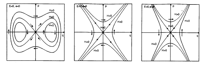
Figure 4: The structure of $H=0$ izolines makes possible the ‘macro-localizations’ for the Zakharov nonlinearity (7.1) with $\varepsilon<0$ and $E<0$; for the case of Gausson a similar picture would be obtained for $\varepsilon<0$ and $E$ arbitrary.

The ‘macro-localizations’ of (2.2) exist if $F(\zeta)=\int f(\zeta)d\zeta$ in $[0,\infty]$ has a proper but local maximum at $\zeta=0$. If this is the case, each canonical orbit of (2.3) emerging from 0 reaches a maximal $q$-value at the intersection of the $I_{\pm}(E)$ line with the $q$-axis, and then returns to 0, drawing a picture of a macro-state. Whether this requires a finite or infinite time depends on the nonlinearity function $f()$. If the time is finite, the system has tendencies to create compact support solutions (droplets), a phenomenon which still awaits investigation (but see an interesting article of Aronson, Crandall and Peletier [13]). Below, we study two cases of (2.2-3) for which the time is infinite (localizations vanish asymptotically as $t\rightarrow\pm\infty$):

$$\text{Classical~{}soliton~{}(Zakharov):}~{}~{}~{}f(\zeta) =\zeta$$ (7.1)

$$\text{Gausson~{}(Bialynicki-Birula~{}\&~{}Mycielski):}~{}~{}~{}f(\zeta) =\ln\zeta$$ (7.2)

The topology of the ‘squeezing lines’ in both cases corresponds to our Fig. 4, though the detailed behaviour of the cues is different. As one can see, the Zakharov eq. has the macro-states for $\varepsilon<0$ and $E<0$; the logarithmic eq. for $\varepsilon<0$ and any $E$. Both integrate easily, leading to the well known formulae:

$${\displaystyle\psi_{S}(x)} =\sqrt{\frac{2E}{\varepsilon}}\frac{1}{\cosh(x\sqrt{-2E})}~{}~{}~{}{\rm(Classical~{}soliton)},$$ (7.3)

$${\displaystyle\psi_{G}(x)} =\exp\left(\frac{E+\varepsilon}{2\varepsilon}+\varepsilon x^{2}\right)~{}~{}~{}{\rm(Gausson)}.$$ (7.4)

The links between the solitons and completely integrable mechanical systems have been carefully explored [28, 29], though the attention was usually focused on the soliton stability (with few exceptions; see, e.g. [45]). For gaussons (7.4) the stability problem is still open. The questions as to, how the soliton (gausson) interacts with an external potential was almost neglected: and this is precisely where the bifurcations occur. In fact, consider the canonical trajectory of eqs. (2.3) which departs from $q=0$ at $t=-\infty$ and draws a macrostate. Suppose, however, the process is perturbed by a little potential pulse $V(t)=\lambda\phi(t)$, where $\lambda\in R$ and $\phi(t)\not\equiv 0$ is a fixed, bounded, non-negative function vanishing outside of a finite interval $(\alpha,\beta)$. One might expect that if $\varepsilon$ is small enough, the existence of $V(t)$ will cause just a little modification in the form of each macrostate. In general though, this is not the case. Indeed one can show that even a very tiny potential pulse can preclude completely the existence of a class of stationary states which exist in vacuum.

Let $I_{\pm}(E)$ be the macrostate loop for (4.3-4) and let ${\bf q}(t)=(q(t),p(t))$ be one of the corresponding localized solutions defined by (4.5). To fix attention, choose ${\bf q}(t)$ on the upper branch $I_{+}(E)$, with $p(t)>0$ and $q(t)$ increasing from 0 to $q_{\rm max}=q(t_{o})$, (where $q_{\rm max}$ is the maximal value of $q$ at the turning point between $I_{+}(E)$ and $I_{-}(E)$). Suppose, the potential pulse $V(t)=\lambda\phi(t)$ occurs in an interval $(\alpha,\beta)$ where ${\bf q}(\alpha),{\bf q}(\beta)\in$ $I_{+}(E)$, $0<q(\alpha),q(\beta)<q_{\rm max}$, $0<p(\alpha),p(\beta)$. Then:

Proposition 3.

If $|\lambda|$ is small enough, $\lambda\neq 0$, then eqs. (3.4) have no bound state coinciding with ${\bf q}(t)$ for $t\leq\alpha$.

Proof.

Let $\tilde{{\bf q}}(t)$ be the integral trajectory of (3.4) for $V(t)=\lambda\phi(t)$ with $\tilde{{\bf q}}(\alpha)={\bf q}(\alpha)$. If $\lambda$ is small enough , then $\tilde{{\bf q}}(t)$ is arbitrarily close to ${\bf q}(t)$ in $(\alpha,\beta)$ together with its 1-st derivative. In particular, $\tilde{q}(\beta)$ must be close to $q(\beta)\Rightarrow 0<\tilde{q}(\beta)<q_{\rm max}$. Moreover, for $t\in(\alpha,\beta),$ $\tilde{{\bf q}}(t)$ intersects each vertical line $q=const$ exactly once, suggesting q as a convenient integration variable to compare both trajectories. Consider therefore the $q$-interval [$q_{\rm 1},q_{\rm 2}$] where $q_{\rm 1}=q(\alpha)=\tilde{q}(\alpha),q_{\rm 2}=\tilde{q}(\beta)$ and compare $\tilde{p}(q_{\rm 2})$ and $p(q_{\rm 2})$. The canonical eqs. (3.4) imply:

$$\frac{dp}{dq}=\frac{-2Eq+2\varepsilon f(q^{2})q}{p},~{}~{}~{}\frac{d\tilde{p}}{dq}=\frac{-2Eq+2\varepsilon f(q^{2})q+2\lambda\phi(t(q))q}{\tilde{p}}$$ (7.5)

$$\frac{d}{dq}\left(\frac{\tilde{p^{2}}}{2}-\frac{p^{2}}{2}\right)=2\lambda\phi(t(q))q\Rightarrow\frac{\tilde{p}(q_{\rm 2})^{2}}{2}-\frac{p(q_{\rm 2})^{2}}{2}=2\lambda\int_{q_{\rm 1}}^{q_{\rm 2}}\phi(t(q))qdq.$$ (7.6)

If now $\lambda>0$ then ${\tilde{p}}(q_{\rm 2})>p(q_{\rm 2})$ and the point $(q_{\rm 2},{\tilde{p}}(q_{\rm 2}))=\tilde{{\bf q}}(\beta)$ ends up in the outer region of the loop $I_{\pm}(E).$ To the contrary, if $\lambda<0$ and $|\lambda|$ small, then $\tilde{{\bf q}}(\beta)$ falls into the interior of the loop. In both cases, ${\bf q}(\beta)$ for $t\geq\beta$ originates a periodic trajectory which circulates either in the external or internal region, without ever returning to 0. ∎

Intuitively, no matter the value of $E$, there is no localization (macrostate) with an infinitesimal pulse under one of its cues. The presence of $V(t)$, (no matter how tiny) must displace the orbit out of the ‘squeezing lemniscate’ $I=I_{\pm}(E)$, creating an unlimited trajectory and a class of macrostates disappears, (a ‘delicate condition’ of macrostates due to the fact that they exist on the threshold of the symmetry breaking. Note that, our proposition adds only some details to the sequence of theorems on the perturbations of homoclinic orbits (see [36, Sec. 4.5] and the literature given there). The recent results in the theory of Bose condensation [41, 42, 43, 44, 45] are interpretable as an indirect consequence of the same mathematical theorems [36].

A macrostate can survive the perturbation if the ‘little obstacle’ is under its ‘mass center’. Geometrically, it means that the pulse $V(t)$ just modifies the outer part of $I_{\pm}(E)$ in vicinity of $q_{\rm max}$. It can also create a bi-localized state by establishing a bridge between two upper or two lower branches of $I_{\pm}(E)$ (see Fig. 5). As a result, the entire ‘macrostate park’ is different in presence of an arbitrarily small $V(t)$.

The metamorphosis is even more radical in presence of two little and widely separated potential pulses, $V(t)=V_{1}(t)+V_{2}(t)$, too small to have any bound states in the traditional sense. Indeed, consider again a classical trajectory which starts to ‘paint a macrostate’ to the left of the left pulse $V_{1}$. Then it may happen that $V_{1}$ deflects the ‘classical point’ (4.2-3) from the lemniscate $I_{\pm}(E)$, to the internal (or external) loop $H$=const, where it starts to circulate, but the second pulse $V_{2}$, turns it back to $I_{\pm}(E)$ where it is finaly driven to 0. The resulting macrostate has the form of a multi-localization, a stationary state which could not exist at all in the collection of vacuum states. Now, it is created just by two tiny ‘potential clips’ (see Fig. 5). Since the stationary states are natural reference points for the general motion, one might expect that a bifurcation in the sets of macrostates must also affect the evolution of nonstationary packets. We shall see below that this is indeed the case.

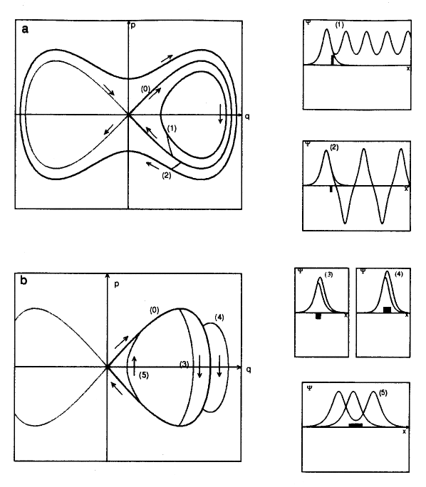
Figure 5: The dynamical symmetry breaking caused by an arbitrarily tiny pulse $V(t)$ makes impossible the existence of a macrostate with $V(t)$ under one of the cues: (1) a little positive $V(t)$ (potential barrier) applied to the canonical trajectory departing from the origin at $t=-\infty$ kicks the trajectory into the internal closed loop $H$ = const $<$ 0, where it starts to circulate endlessly without returning to the origin. (2) a negative $V(t)$ (potential well) pushes. the trajectory toward an external lemniscate $H$ = const $>$ 0, where it again circulates, without returning to the origin. (3-4) The macrostates with $V(t)$-pulse collocated under the center of the wave packet are possible either for the well or barrier. (5) A new macrostate in form of a bi-localization can be also created by arbitrarily tiny potential pulse.

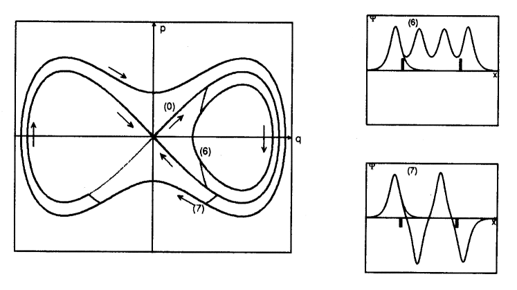
Figure 6: A pair of arbitrary weak barriers (wells) permits the multi-soliton states: (6) a multisoliton created by several circulations of the classical trajectory on the internal $H$-curve, ‘clipsed’ by two tiny potential barriers, (7) an analogous multi-soliton created by an external circulation, is maintained by two tiny wells.

8 The non-stationary states.

The stationary solutions have a guiding role in linear theories. Would the same be true in the non-linear case? To check this we have returned to (2.1) and applied numerical techniques to examine some general, non-stationary waves $\Psi(x,t)$ (with $t$ meaning again the time and $x$ the space coordinate). We were specially curious to see what happens to the initial macrostate (7.3) or (7.4) in presence of a very little potential pulse $V(x)$:

$$V(x)=\left\{\begin{array}[]{l}{\displaystyle V_{o}\left[1-\frac{(x-x_{v})^{2}}{\sigma^{2}}\right]^{2},~{}~{}~{}|x-x_{v}|\leq\sigma}\\[4.30554pt] 0,~{}~{}~{}|x-x_{v}|>\sigma\end{array}\right.$$ (8.1)

We have first taken a small $V_{o}<0$ and $x_{v}<0$, to represent a little potential well situated under the left vanishing cue of the initial macrostate, and we have examined the evolution of the packet $\Psi(x,t)$ in the initial form of Gausson for the non-linearity (7.2). The result is curious: the packet $\Psi(x,t)$ is first attracted toward the well, then starts to perform around it a sequence of decaying oscillations loosing an ‘excess of matter’ and tending slowly to a new equilibrium state (of smaller norm), right on the center of the well; see Fig. 7a. Its asymptotic form is therefore affected by an arbitrarily small $|V_{o}|$. The similar effect is observed for the Zakharov soliton, see Fig. 7b-e. Evidently, while there is no discontinuity of the finite time evolution of the soliton (Gausson) due to the influence of $V(t)$ there is a discontinuity (bifurcation) in its asymptotic form (meaning that the limiting transitions $V\rightarrow 0$ and $t\rightarrow+\infty$ do not commute).

Our next experiment involved the Gausson initially situated almost upon the center of a little potential barrier. As turns out the simulation can generate several scenarios, the most interesting one is the Gausson splitting illustrated on Fig. 8c. (In our computer simulations we also observed an analogous phenomenon for the traditional Zakharov soliton). The splitting occurs as well for the traveling soliton of the initial form,

$$\Psi(x,0)=\psi_{S}(x)\exp(ikx),$$ (8.2)

colliding with the potential barrier (where $\psi_{S}$ is given by 7.3). As turns out, the too slow soliton is totally reflected and too quick soliton is totally transmitted, Fig. 9; the splitting occurs for intermediate packet velocities. We conclude that the solitons, while stable in mutual collisions, can loose stability in presence of external potentials.

Our last experiment was to examine the influence of two tiny potential wells placed symmetrically under two cues of the initial Zakharov soliton. Our calculations show that the bi-soliton stationary state (Fig. 6) dictates the asymptotic form of the non-stationary wave $\Psi(x,t)$, see Fig. 10. We thus see that while a tiny pulse of the external potential cannot affect the continuity of the macrostate evolution, it can however cause the bifurcation of their asymptotic forms consistently with our idea of the non-linear spectral phenomenon. It is interesting to notice, that the bifurcations which we are describing arised already in some applied areas. Thus, the metamorphosis of the localized stationary state into a ‘respiring lump’ resembles phenomenon predicted in physics of boson condensation (see [43]); likewise the split soliton seems an abstract equivalent of an effect discused in [44], both belonging to the newly emerging side of the soliton theory.

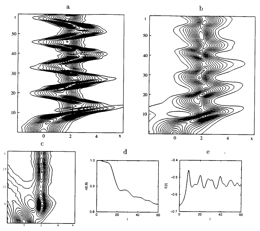
Figure 7: Effects of a little well (8.1) placed under the cue of ‘macrostate’ $\Psi(x,0)$. The evolving packet represented by the izolines of $|\Psi(x,t)|^{2}$ tries to find an equilibrium state upon the center of the well (eq., $x_{v}$ = 2, $\sigma$ = 0.5, $V_{o}$ = -0.75): (a) $\Psi(x,0)$ is a Gausson (7.4); (b) $\Psi(x,0)$ represents the soliton in Zakharov equation (7.3); (c) a detail of the Zakharov process (for $V_{o}$ = -2) shows probable emission of a part of the soliton substance when tending to an equilibrium state; (d) the time evolution of the partial norm $n_{[-8,10]}(t)$ eq. (A.3) confirms the previous conclusion; (e) the generalized frequency parameter $E$ given by (A.4) tends to a new value for the new equilibrium state.

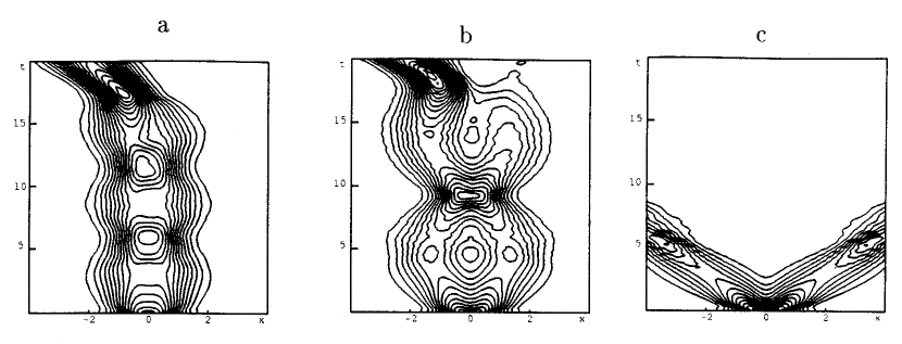
Figure 8: Cases of Gausson evolution in presence of the barrier (8.1) centered almost at the maximum of the initial $\Psi(x,0)$ ($x_{v}$ = 0.001, $\sigma$ = 0.5). (a) For low $V_{o}$ = 0.5 the Gausson hesitates but than deflects to the left without loosing integrity, (b) an analogue phenomenon for $V_{o}$ = 1 suggests an emission of the Gausson substance, (c) the barrier $V_{o}$ = 2 causes the new phenomenon of Gausson splitting.

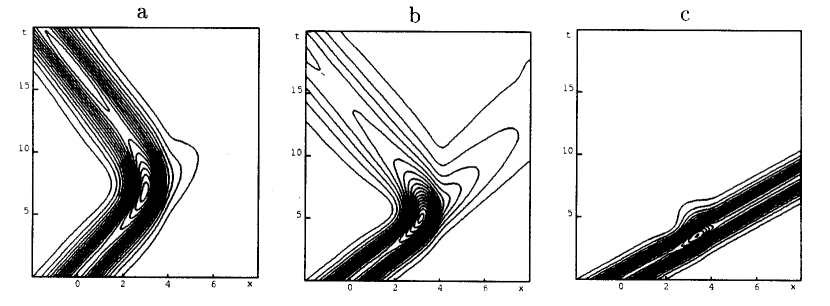
Figure 9: The evolution of the Zakharov soliton $\Psi(x,0)=\psi_{Z}(x)\exp(ikx)$ colliding with the potential barrier of form (8.1) with $x_{v}$=4, $\sigma$ = 0.5: (a) for $k$ = 0.5, $V_{o}$ = 1 the soliton is totally reflected; (b) for $k$ = 0.7, $V_{o}$ = 1 the soliton splits; (c) for a slightly faster soliton $k$ = 1 and lower barrier $V_{o}$ = 0.5 the packet is totally transmitted.

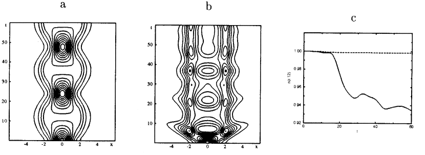
Figure 10: The evolution of the Zakharov ‘macrostate’ (8.2) in presence of two potential wells of form (eq. , $\sigma$ = 0.5) placed at $x=\pm 2$: (a) for $V_{o}$ = -0.5 the packet performs quadrupole oscillations around wells; (b) for $V_{o}$ = -1 it appears to tend to the stationary bi-soliton state; (c) the partial norms of the soliton $n_{[-12,12]}(t)$ for the both processes suggests that the new equilibrium in the case (b) is achieved at the cost of emitting an excess of substance.

Appendix: Numerical Algorithms

For numerical solution of the equation (2.1) we apply a very simple discretization of the space and time preserving the fundamental symplectic character of the dynamics. The equation is represented in form of the classical Hamiltonian equations for a continuous medium,

$$\frac{\partial Q}{\partial t}=\frac{\delta{\cal H}}{\delta P},~{}~{}~{}\frac{\partial P}{\partial t}=-\frac{\delta{\cal H}}{\delta Q}.$$ (A.1)

The real numbered functions $Q(x,t)$ and $P(x,t)$ represent real and imaginary part of $\Psi(x,t)$ and ${\cal H}$ is the following functional,

$${\cal H}\left[Q,P\right]=\frac{1}{2}\int\left[-\frac{Q}{2}\frac{d^{2}Q}{dx^{2}}-\frac{P}{2}\frac{d^{2}P}{dx^{2}}+(Q^{2}+P^{2})V+\varepsilon F(Q^{2}+P^{2})\right]dx.$$ (A.2)

Note that values of ${\cal H}$ and of the norm of the wave function are preserved in the evolution. The functions $Q$ and $P$ are represented on the finite regular grid of points in the domain of $x$ and the Laplacian is approximated with a finite difference formula. Consistently, the equations (A.1) are transformed into ordinary Hamiltonian equations for many degrees of freedom. In practice we apply the grid $x\in[-16,16]$ with 801 points. An appropriately extended grid is required for simulations of the traveling packets. In all cases where the emission of the ‘packet substance’ is reported we additionally applied the technique of absorbing boundaries on the edges of the grid. This representation does not produce any substantial artifacts of the space discretization. For the time integration we use the implicit second order Range-Kutta method which is strictly symplectic and appropriate for classical Hamiltonians which are not separable into a kinetic and potential part [46]. The integration time step is $2\times 10^{-4}$ ensuring absolute stability and elimination of any substantial artifacts of the time discretization. In order to analyze the evolution of the packet we introduce the norm $N$ and the partial norm $n_{L}$:

$$n_{L}(t)=\frac{1}{N}\int_{L}|\Psi(x,t)|^{2}dx,~{}~{}~{}N=\int|\Psi(x,t)|^{2}dx,$$ (A.3)

and the field functional $E(t)$ generalizing the eigenvalue $E$ of (3.2) to the nonstationary solutions,

$$E(t)=\frac{1}{N}\int\Psi^{\ast}(x,t)\left[-\frac{1}{2}\frac{\partial^{2}}{\partial x^{2}}+V(x)+\varepsilon f(|\Psi(x,t)|^{2})\right]\Psi(x,t)dx.$$ (A.4)

The simulations have been performed with help of the fortran program with 48-bits representation of real numbers running on Cray Y-MP/4E.

References

- [1] R. Haag and U. Bannier, Commun. Math. Phys 60, 1 (1978)
- [2] T. W. Kibble, Commun. Math. Phys 64, 73 (1978); 65, 189 (1979); J. Phys. A 13, 141 (1980)
- [3] I. Bialynicki-Birula and J. Mycielski, Ann. Phys. 100, 62 (1976)
- [4] S. Weinberg, Ann. Phys. 194, 336 (1989)
- [5] M. Czachor, Found. Phys. Lett. 4, 351 (1991)
- [6] M. Czachor, Phys. Rev. A 53, 1310 (1996); Phys. Lett. A 225, 1 (1997).
- [7] H. D. Doebner and G. A. Goldin, Phys. Lett. A 162, 397 (1992)
- [8] H. D. Doebner and G. A. Goldin, J. Phys. A 27, 1771 (1994)
- [9] V. V. Dodonov and S. S. Mizrahi, J. Phys. A 26, 7163 (1993); Ann. Phys. 237, 226 (1995)
- [10] E. Diez, F. Dominguez-Adame and A. Sanchez, Phys. Lett. A 198, 403 (1995); A 215, 103 (1996).
- [11] M. Grabowski and P. Hawrylak, Phys. Rev. B 41, 5783 (1990)
- [12] B. Mielnik, Commun. Math. Phys 31, 221 (1974)
- [13] D. Aronson, M. G. Crandall, L.A. Peletier, Nonlinear Analysis, Theory, Methods , Application, 6, 1001 (1982)
- [14] P. Nattermann, in Physical Applications and Mathematical Aspects of Geometry, Groups, and Algebras, H.-D. Doebner, P. Nattermann and W. Scherer Eds., World Scientific, Singapore (1997), pp. 428-432; P. Nattermann, in Symmetry and Science IX, B. Gruber Ed., Plenum Pub., New York (1997), to appear.
- [15] N. Gisin, J. Phys. A 14, 2259 (1981); J. Math. Phys 24, 1779 (1983); J. Phys. A 19, 205 (1986)
- [16] N. Gisin, Helv. Phys. Acta 62, 363 (1989); Phys. Lett. A 143, 1 (1990); N. Gisin and M. Rigo, J.. Phys. A 28, 7375 (1995)
- [17] H. Spohn, Rev. Mod. Phys. 53, 569 (1980)
- [18] F. Capasso and S. Datta, Phys. Today 43 (2) 74 (1990)
- [19] H. J. C. Berendsen and J. Mavri, J. Phys. Chem. 97, 13464 (1993)
- [20] P. Bala, P. Grochowski, B. Lesyng and J. A. McCammon, J. Phys. Chem. 100, 2535 (1996)
- [21] F. Brauer, J. Math. Anal. Appl. 22, 591 (1968)
- [22] H. Prüfer, Math. Annalen 95, 409 (1926)
- [23] A. Malkin and V. I. Manko, JETP 31, 386 (1970)
- [24] S. Coleman, Aspects of Symmetry, CUP, London (1985)
- [25] D. Sanjines C. , Rev. Mex. Fis. 36, 181 (1990)
- [26] I. Bialynicki-Birula, M. Cieplak and J. Kaminski, Theory of Quanta, OUP, New York-Oxford (1992)
- [27] B. Mielnik and M. A. Reyes, J. Phys. A 29, 6009 (1996); M. A. Reyes and H. C. Rosu, Phys. Rev. E, 57, 4850 (1998)
- [28] S. Rauch-Wojciechowski, Phys. Lett. A 160, 241 (1991); A 170, 91 (1992); S. Rauch-Wojciechowski, Chaos, Solitons & Fractals 5, 2235 (1995)
- [29] S. Rauch-Wojciechowski and M. Blaszak, Physica A 197, 191 (1993)
- [30] J. E. Avron and B. Simon, Phys. Rev. Lett. 46, 1166 (1981)
- [31] P. Rabinovitz, Comm. Pure Appl. Math 23, 939 (1970) J. Funct. Anal. 7, 487 (1971)
- [32] M. Eastbrooks and J. Macki, J. Diff. Equ. 10, 1083 (1971)
- [33] R. Turner, J. Diff. Equ. 10, 141 (1971)
- [34] G. Gustafson and K. Schmitt, J. Diff. Equ. 12, 129 (1972)
- [35] E. F. Hefter, Lett. Nuovo Cimento 32, 9 (1981); Nouv. Cim. 59 A, 275 (1980); Phys. Rev. A 32, 1201 (1985)
- [36] J. Guckenheimer, P.Holms, Nonlinear Oscillations, Dynamical Systems, and Bifurcations of Vector Fields Springer-Verlag, New York (1983)
- [37] J. Klauder, Metrical Quantization in Quantum Future, From Volta and Como to Present and Beyond, Proceedings of Xth Max Born Symposium Held in Przesieka, Poland, 24-27 September 1997, p. 129–138, eds. A. Jadczyk and P. Blanchard, Springer-Verlag 1997, ISBN 978-3-540-65218-2
- [38] Ying-kai Wu and Bambi Hu Phys. Rev. A 35, 1404 (1987)
- [39] Sang-Yuun Kim and Bambi Hu, Phys. Rev. A 38, 1534 (1988)
- [40] V. E. Zakharov, L. D. Faddeev, Funct. Anal. Appl. 5, 18 (1971); V. E. Zakharov, A. B. Shabat, Funct. Anal. Appl. 8, 43 (1974)
- [41] F. Dalfovo, L. Pitaevskii and S.Stringari J.Res.Natl.Inst.Stand. Technol. 101, 537 (1996) C.C. Bradley, C.A. Sackett, R.G. Hulet Phys. Rev. Lett 78, 985 (1997)
- [42] M. Ueda a. J. Leggett, Phys. Rev. Lett. 80 1576 (1998)
- [43] C.A. Sackett, C.C. Bradley, M.Welling, R.G. Hulet Appl. Phys. B 65, 433-440 (1997)
- [44] R. Dum, A. Sanpera, K.A. Suominen, M. Kus, K. Rzazewski, M. Lewenstein Phys. Rev. Lett. 80, 3899 (1998)
- [45] I. V. Bareshenkov, Phys. Rev. Lett 77, 1193 (1996)
- [46] J. M. Sanz-Serna Numerical Hamiltonian Systems (Chapman and Hall, London, Glasgow, New York, Tokyo, 1994)