Resonance fluorescence from an asymmetric quantum dot dressed by a bichromatic electromagnetic field

Abstract

We present the theory of resonance fluorescence from an asymmetric quantum dot driven by a two-component electromagnetic field with two different frequencies, polarizations and amplitudes (bichromatic field) in the regime of strong light-matter coupling. It follows from the elaborated theory that the broken inversion symmetry of the driven quantum system and the bichromatic structure of the driving field result in unexpected features of the resonance fluorescence, including the infinite set of Mollow triplets, the quench of fluorescence peaks induced by the dressing field, and the oscillating behavior of the fluorescence intensity as a function of the dressing field amplitude. These quantum phenomena are of general physical nature and, therefore, can take place in various double-driven quantum systems with broken inversion symmetry.

I Introduction

Advances in nanotechnology, laser physics and microwave techniques created a basis for studies of the strong light-matter coupling in various quantum systems. Differently from the case of weak electromagnetic field, the interaction between electrons and a strong field cannot be treated as a perturbation. Therefore, the system “electron + strong field” is conventionally considered as a composite electron-field object which was called “electron dressed by field” (dressed electron) Cohen-Tannoudji_b98 ; Scully_b01 . The field-induced modification of physical properties of dressed electrons was studied in both atomic systems Cohen-Tannoudji_b98 ; Scully_b01 ; Autler_55 and various condensed-matter structures, including bulk semiconductors Elesin_69 ; Vu_04 ; Vu_05 , graphene Lopez_08 ; Kibis_10 ; Kibis_11_1 ; Glazov_14 ; Usaj_14 , quantum wells Mysyrovich_86 ; Wagner_10 ; Kibis_12 ; Teich_13 ; Shammah ; Barachati , quantum rings Kibis_11 ; Kibis_13 ; Joibari_14 ; Kyriienko_15 , quantum dots Reithmaier ; Yoshie ; Bloch_2005 ; Muller_2007 ; Kibis_09 ; Ulrich_2011 ; Majumdar_2012 ; Savenko_2012 ; Oster_2012 ; Paspalakis_2013 ; Schneider_2015 , etc. Among these structures, quantum dots (QDs) — semiconductor 3D structures of nanometer scale, which are referred to as “artificial atoms” — seem to be most interesting for optical studies since they are basic elements of modern nanophotonics Masumoto_book ; Tartakovskii_book . In contrast to natural atoms, the most of QDs are devoid of inversion symmetry and, therefore, are asymmetric. As an example, QDs based on gallium nitride heterostructures have a strong built-in electric field Widmann_98 ; Moriwaki_00 and, therefore, acquire the giant anisotropy Williams_05 ; Bretagnon_06 ; Warburton_2002 ; Ostapenko_2010 ; Ostapenko_2013 . This motivates to studies of various asymmetry-induced optical effects in QDs Kibis_09 ; Savenko_2012 ; Oster_2012 ; Paspalakis_2013 .

The most of studies of dressed quantum systems was performed before for a monochromatic dressing field. However, there is a lot of interesting phenomena specific for quantum systems driven by a two-mode electromagnetic field with two different frequencies, polarizations and amplitudes (bichromatic field). In symmetric quantum systems (atoms and superconducting qubits), the bichromatic coupling leads to features of photon correlations, squeezing, Autler-Townes effect, suppression of spontaneous emission, multi-photon transitions, etc. Ficek_96 ; Kry1 ; Kry2 ; Kry3 ; Ficek_99 ; Kry4 ; Ramirez_2013 ; Shevchenko_2014 . Broken symmetry brings substantially new physics to bichromatically dressed quantum systems, including additional lines in optical spectra, multiple splitting of the dressed-state transitions, etc. Freedhoff_1975 ; Windsor_1998 ; Macovei_2015 . Although these optical effects are extensively studied during long time, a consistent quantum theory of resonance fluorescence from bichromatically dressed asymmetric systems was not elaborated before. The present research is aimed to fill this gap at the border between quantum optics and physics of nanostructures. To solve the problem, we focused on the strong light-matter coupling regime when the interaction of an asymmetric QD with a bichromatic dressing field overcomes the spontaneous emission and non-radiative decay of QD excitations. In this case, the spectral lines of QD are well resolved and various radiation effects (particularly, the resonance fluorescence) can be analyzed using a concept of quasienergetic (dressed) electronic states. In the framework of this approach, such characteristics of dressed QD as decay rates and lineshapes can be calculated by solving the master equations in the representation of quasienergetic states. As a result, we found unexpected features of resonance fluorescence, which are discussed below.

The paper is organized as follows. In the Section II, we derive quasienergetic electronic states for an asymmetric QD dressed by a bichromatic electromagnetic field and calculate matrix elements of optical dipole transitions between these states. In the Section III, we apply the found quasienergetic spectrum of dressed electrons to elaborate the theory of resonance fluorescence from the QD. The Section IV contains the discussion of the calculated spectra of resonance fluorescence and the conclusion.

II Model of electronic structure

Let us consider an asymmetric QD with broken inversion symmetry along the $z$ axis, which is dressed by the bichromatic field

$$\mathbf{E}(t)=\mathbf{E}_{1}\cos\omega_{1}t+\mathbf{E}_{2}\cos\omega_{2}t,$$ (1)

where the electric field of the first mode, $\mathbf{E}_{1}$, is directed along the $z$ axis and the electric field of the second mode, $\mathbf{E}_{2}$, is perpendicular to this axis (see Fig. 1a). In what follows, we will assume that the second frequency, $\omega_{2}$, is near the electronic resonance frequency, $\omega_{0}$, whereas the first frequency, $\omega_{1}$, is far from all resonance frequencies. As a consequence, the bichromatic field (1) mixes effectively only two electron states of QD, $|1\rangle$ and $|2\rangle$, which are separated by the energy $\hbar\omega_{0}$ (see Fig. 1b). Within the basis of these two states, the asymmetric QD can be described by the matrix Hamiltonian Kibis_09

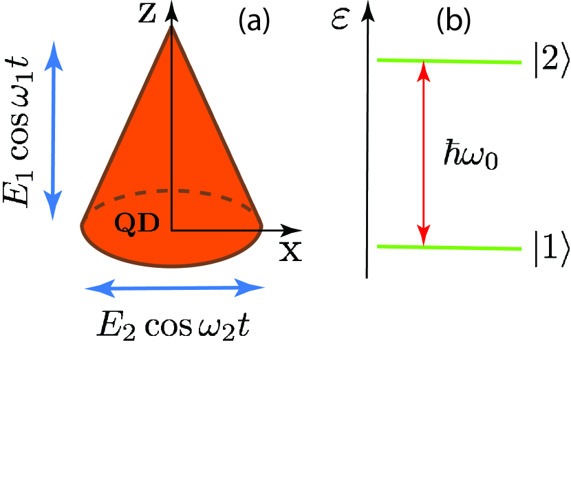
Figure 1: (Color online) Sketch of the system under consideration: (a) Asymmetric quantum dot (QD) with broken inversion symmetry along the $z$ axis, which is exposed to a bichromatic electromagnetic field with the electric field amplitudes $E_{1,2}$ and the frequencies $\omega_{1,2}$; (b) Two-level model of the electronic energy spectrum of the QD, $\varepsilon$, with the interlevel distance $\hbar\omega_{0}$.

$$\hat{\cal H}=\begin{pmatrix}-\hbar\omega_{0}/2-{d}_{11}{E}_{1}\cos\omega_{1}t&-{d}_{12}{E}_{2}\cos\omega_{2}t\\ -{d}_{21}{E}_{2}\cos\omega_{2}t&\hbar\omega_{0}/2-{d}_{22}{E}_{1}\cos\omega_{1}t\end{pmatrix}$$ (2)

where ${d}_{11}=\langle 1|ez|1\rangle$, ${d}_{22}=\langle 2|ez|2\rangle$ and ${d}_{12}={d}_{21}=\langle 1|ex|2\rangle$ are the matrix elements of the operator of electric dipole moment along the $z,x$ axes, and $e$ is the electron charge. To simplify calculations, the Hamiltonian (2) can be written as a sum, $\hat{\cal H}=\hat{\cal H}_{0}+\hat{\cal H}^{\prime}$, where

$$\hat{\cal H}_{0}=\begin{pmatrix}-\hbar\omega_{0}/2-{d}_{11}{E}_{1}\cos\omega_{1}t&0\\ 0&\hbar\omega_{0}/2-{d}_{22}{E}_{1}\cos\omega_{1}t\end{pmatrix}$$ (3)

is the diagonal part of the full Hamiltonian (2), and

$$\hat{\cal H}^{\prime}=\begin{pmatrix}0&-{d}_{12}{E}_{2}\cos\omega_{2}t\\ -{d}_{21}{E}_{2}\cos\omega_{2}t&0\end{pmatrix}$$ (4)

is the nondiagonal part describing electron transitions between the states $|1\rangle$ and $|2\rangle$ under influence of the field (1). Exact solutions of the non-stationary Schrödinger equation with the Hamiltonian (3),

$$i\hbar\frac{\partial\psi}{\partial t}=\hat{\cal H}_{0}\psi,$$

can be written in the spinor form as

$$\psi^{(-)}=e^{i\omega_{0}t/2}\exp{\left[i\frac{{d}_{11}{E}_{1}}{\hbar\omega_{1}}\sin\omega_{1}t\right]}\begin{pmatrix}1\\ 0\end{pmatrix}$$ (5)

and

$$\psi^{(+)}=e^{-i\omega_{0}t/2}\exp{\left[i\frac{{d}_{22}{E}_{1}}{\hbar\omega_{1}}\sin\omega_{1}t\right]}\begin{pmatrix}0\\ 1\end{pmatrix}.$$ (6)

Since the two pseudo-spinors (5)–(6) are the complete basis of the considered electronic system at any time $t$, we can sought eigenstates of the full Hamiltonian (2) as an expansion

$$\widetilde{\psi}=a^{(-)}(t)\psi^{(-)}+a^{(+)}(t)\psi^{(+)},$$ (7)

where the time-dependent coefficients $a^{(\pm)}(t)$ obey the equation

$$i\hbar\dot{a}^{(\mp)}(t) = -a^{(\pm)}(t){d}_{12}{E}_{2}\cos\omega_{2}te^{\mp i\omega_{0}t}$$ (8)

$$\times \exp\left[\pm i\frac{({d}_{22}-{d}_{11}){E}_{1}}{\hbar\omega_{1}}\sin\omega_{1}t\right].$$

Applying the Jacobi-Anger expansion,

$$e^{iz\sin\theta}=\sum_{n=-\infty}^{\infty}J_{n}(z)e^{in\theta},$$

we arrive from Eq. (8) at the equation

$$i\hbar\dot{a}^{(\mp)}(t) = -a^{(\pm)}(t)\frac{{d}_{12}{E}_{2}}{2}\sum_{n=-\infty}^{\infty}J_{n}\left(\frac{({d}_{22}-{d}_{11}){E}_{1}}{\hbar\omega_{1}}\right)$$ (9)

$$\times \left[e^{\mp i(\omega_{0}+\omega_{2}-n\omega_{1})t}+e^{\mp i(\omega_{0}-\omega_{2}-n\omega_{1})t}\right],$$

where $J_{n}(z)$ is the Bessel function of the first kind. Formally, the equation of quantum dynamics (9) describes a two-level quantum system subjected to a multi-mode field. It is well-known that the main contribution to the solution of such equation arises from a mode which is nearest to the resonance. Correspondingly, near the resonance condition,

$$\omega_{0}\pm\omega_{2}=n\omega_{1},$$ (10)

we can neglect all modes except the resonant one. In this approximation, Eq. (9) reads as

$$i\dot{a}^{(\pm)}(t)=a^{(\mp)}(t)F_{n}e^{\pm i\varphi_{n}t},$$ (11)

where $F_{n}=-({{d}_{12}{E}_{2}}/{2\hbar})J_{n}\left(\widetilde{\omega}/\omega_{1}\right)$ are the Rabi frequencies of the considered system,

$$\widetilde{\omega}=\frac{E_{1}(d_{22}-d_{11})}{\hbar}$$ (12)

is the effective frequency, and $\varphi_{n}=\omega_{0}\pm\omega_{2}-n\omega_{1}$ is the resonance detuning. It follows from Eq. (11) that the considered problem is reduced to the effective two-level system driven by the monochromatic field with the combined frequency $\varphi_{n}$. Using the well-known solution of Eq. (11) (see, e.g., Ref. [Landau, ]), we can write the sought wave functions (7) in the conventional form of quasienergetic (dressed) states as

$$\widetilde{\psi}_{1} = e^{-i\tilde{\varepsilon}_{1}t/\hbar}\Bigg{[}\sqrt{\frac{1}{2}\left(1+\frac{\varphi_{n}}{2\Omega_{n}}\right)}\Lambda_{11}(t)\begin{pmatrix}1\\ 0\end{pmatrix}$$ (13)

$$- \sqrt{\frac{1}{2}\left(1-\frac{\varphi_{n}}{2\Omega_{n}}\right)}e^{i(\varphi_{n}-\omega_{0})t}\Lambda_{22}(t)\begin{pmatrix}0\\ 1\end{pmatrix}\Bigg{]},$$

$$\widetilde{\psi}_{2} = e^{-i\tilde{\varepsilon}_{2}t/\hbar}\Bigg{[}\sqrt{\frac{1}{2}\left(1+\frac{\varphi_{n}}{2\Omega_{n}}\right)}\Lambda_{22}(t)\begin{pmatrix}0\\ 1\end{pmatrix}$$ (14)

$$+ \sqrt{\frac{1}{2}\left(1-\frac{\varphi_{n}}{2\Omega_{n}}\right)}e^{-i(\varphi_{n}-\omega_{0})t}\Lambda_{11}(t)\begin{pmatrix}1\\ 0\end{pmatrix}\Bigg{]},$$

where

$$\tilde{\varepsilon}_{1}=-\frac{\hbar\omega_{0}}{2}-\hbar\Omega_{n}+\hbar\frac{\varphi_{n}}{2},\,\,\,\,\tilde{\varepsilon}_{2}=\frac{\hbar\omega_{0}}{2}+\hbar\Omega_{n}-\frac{\hbar\varphi_{n}}{2}.$$ (15)

are the corresponding quasienergies and

$$\Lambda_{ii}(t)=\exp{\left[i\frac{{d}_{ii}{E}_{1}}{\hbar\omega_{1}}\sin\omega_{1}t\right]},\,\,\,\,\Omega_{n}=\sqrt{\frac{\varphi_{n}^{2}}{4}+F_{n}^{2}}.$$

As to optical transitions between the dressed states (13) and (14), they can be described by the matrix dipole elements

$$\tilde{{d}}_{ij}(t)=\langle\widetilde{\psi}_{i}|ex|\widetilde{\psi}_{j}\rangle=d_{ij}^{(+)}+d_{ij}^{(-)},$$ (16)

where $d_{ij}^{(+)}=\left[d_{ji}^{(-)}\right]^{*}$,

$$d_{21}^{(+)} = \frac{d_{21}}{2}\left[1+\frac{\varphi_{n}}{2\Omega_{n}}\right]\Lambda^{*}(t)e^{i(\omega_{0}-\varphi_{n}+2\Omega_{n})t},$$

$$d_{21}^{(-)} = -\frac{d_{12}}{2}\left[1-\frac{\varphi_{n}}{2\Omega_{n}}\right]\Lambda(t)e^{-i(\omega_{0}-\varphi_{n}-2\Omega_{n})t},$$

$$d_{11}^{(+)} = -d_{22}^{(+)}=-\frac{d_{12}}{2}\frac{F_{n}}{\Omega_{n}}\Lambda^{*}(t)e^{i(\omega_{0}-\varphi_{n})t},$$ (17)

and $\Lambda(t)=\Lambda_{22}(t)\Lambda_{11}^{*}(t)$.

III Resonance fluorescence

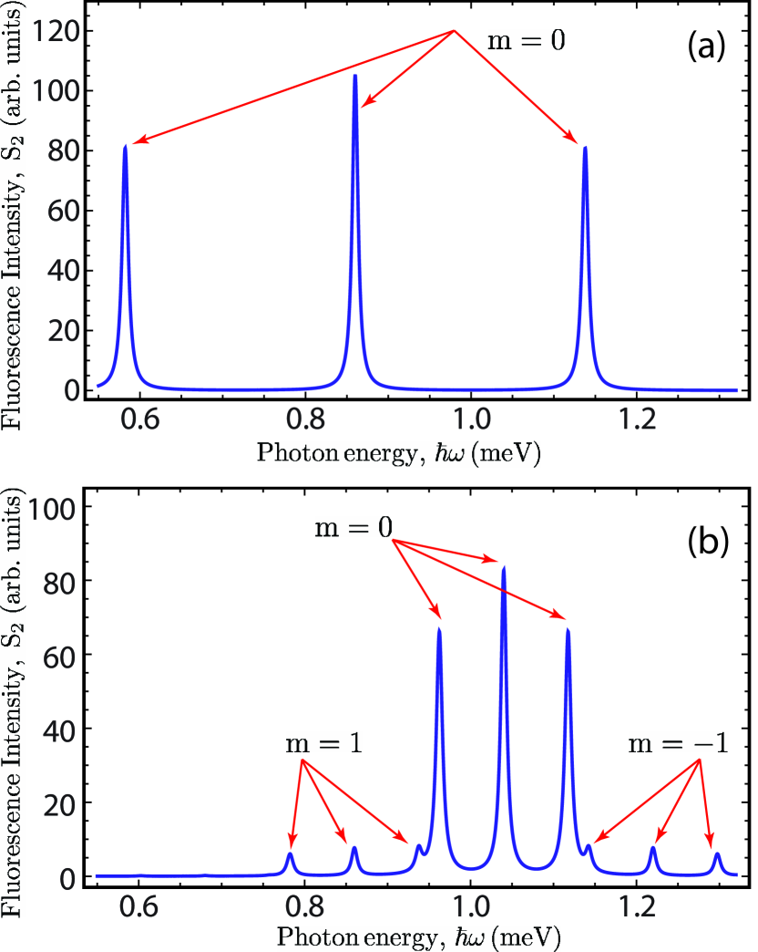
Figure 2: (Color online) The spectra of resonance fluorescence from an asymmetric quantum dot with the interlevel distance $\hbar\omega_{0}=1$ meV, dipole moments $d_{22}-d_{11}=d_{12}=40$ D, and the decay rate $\gamma=10^{-10}$ s^-1: (a) in the presence of a monochromatic dressing field with the amplitude $E_{2}=3\cdot 10^{3}$ V/cm and the frequency $\omega_{2}=0.86\,\omega_{0}$; (b) in the presence of a bichromatic dressing field with the amplitudes $E_{1}=1.3\cdot 10^{3}$ V/cm, $E_{2}=3\cdot 10^{3}$ V/cm and the frequencies $\omega_{1}=0.18\,\omega_{0}$, $\omega_{2}=0.86\,\omega_{0}$. The indices $m=0,\pm 1$ indicate the different Mollow triplets.

The general theory to describe the resonance fluorescence in the representation of quasienergetic (dressed) states has been elaborated in Refs. Cohen ; Scully ; Kry5 ; Kry6 . Applying this known approach to the considered dressed QD, we have to write the Hamiltonian of interaction of the QD with the radiative field as

$$\hat{H}_{\mathrm{int}}=-\tilde{d}_{ij}(t)[\textbf{E}^{+}(t)+\textbf{E}^{-}(t)],$$ (18)

where

$$\textbf{E}^{\pm}(t)=\int d\omega g^{\pm}(\omega)\textbf{e}^{\pm}_{\omega}a^{\pm}_{\omega}e^{\mp i\omega t}$$

is the positive (negative) frequency part of the radiative electric field, $\textbf{E}(t)=\textbf{E}^{+}(t)+\textbf{E}^{-}(t)$, the parameters $g^{\pm}(\omega)$, $\textbf{e}^{\pm}_{\omega}$, $a^{\pm}_{\omega}$ describe the density, polarization and amplitude of the corresponding electromagnetic modes, respectively, and $\tilde{d}_{ij}(t)$ are the dipole matrix elements of dressed QD (16)–(II). Within the conventional secular approximation and Markov approximation Cohen-Tannoudji_b98 , the equations describing the quantum dynamics of the considered two-level system read as

$$\frac{d\sigma_{11}(t)}{dt}=-\Gamma_{11}[\sigma_{11}(t)-\sigma_{11}^{S}],\,\,\,\frac{d\sigma_{12}(t)}{dt}=-\Gamma_{12}\sigma_{12}(t),$$

$$\sigma_{11}(t)+\sigma_{22}(t)=1,$$

where $\sigma(t)=\mathrm{Tr}\left\{\rho(t)\right\}$ is the reduced density operator which involves tracing over reservoir variables, $\sigma_{\alpha\beta}=\langle\widetilde{\psi}_{\alpha}|\sigma|\widetilde{\psi}_{\beta}\rangle$ are the matrix elements of the density operator written in the basis of dressed states (13)–(14),

$$\sigma_{11}^{S}=\frac{w_{21}}{w_{12}+w_{21}},\qquad\sigma_{22}^{S}=\frac{w_{12}}{w_{12}+w_{21}}$$ (19)

are the steady-state populations of the dressed states (13)–(14),

$$\Gamma_{11}=w_{12}+w_{21},\,\,\Gamma_{12}=\frac{\Gamma_{11}}{2}-\mathrm{Re}(M_{11,22}+M_{22,11})$$ (20)

are the field-dependent decay rates for the dressed states (13)–(14),

$$w_{12}=\frac{\gamma}{4}\left(1-\frac{\varphi_{n}}{2\Omega_{n}}\right)^{2},\,\,\,\,w_{21}=\frac{\gamma}{4}\left(1+\frac{\varphi_{n}}{2\Omega_{n}}\right)^{2}$$ (21)

are the probabilities of radiative transitions per unit time between the dressed states (13)–(14),

$$M_{\alpha,\alpha,\beta,\beta}=\int\limits_{0}^{\infty}\mathrm{d}\tau\,\widetilde{d}_{\alpha\alpha}(t-\tau)\widetilde{d}_{\beta\beta}(t)\langle E(t)E(t-\tau)\rangle,$$ (22)

$\langle E(t)E(t-\tau)\rangle$ is the correlation function averaged over the initial state of electromagnetic field, and $\gamma$ is the spontaneous emission rate. Substituting Eqs. (21)–(22) into Eqs. (19)–(20), we arrive at the width of the transitions,

$$\Gamma_{11}=\frac{\gamma}{2}\left(1+\frac{\varphi_{n}^{2}}{4\Omega_{n}^{2}}\right),\,\,\,\,\Gamma_{12}=\frac{\gamma}{4}\left(3-\frac{\varphi_{n}^{2}}{4\Omega_{n}^{2}}\right),$$ (23)

and the difference between the populations of dressed electronic states (13)–(14),

$$\Delta_{S}=\sigma_{11}^{S}-\sigma_{22}^{S}=2w_{21}/\Gamma_{11}-1.$$ (24)

Taking into account the aforesaid, the spectrum of resonance fluorescence from QD has the form Scully_b01

$$S(\omega)\sim\frac{1}{\pi}\mathrm{Re}\left\{\int\limits_{0}^{\infty}d\tau\langle D^{(+)}(t+\tau)D^{(-)}(t)\rangle e^{-i\omega\tau}\right\},$$ (25)

where

$$D^{(\pm)}(t)=\sum\limits_{\alpha,\beta}\sigma_{\alpha\beta}(t)d^{(\pm)}_{\alpha\beta}(t)$$ (26)

is the positive(negative)-frequency part of the polarization operator written in the basis of dressed states (13)–(14). Applying the quantum regression theorem Scully_b01 and taking into account Eqs. (16)–(II), we arrive at the correlation function of the polarization operator (26) in the steady-state regime for long time $t$ and arbitrary time $\tau$,

$$\langle D^{(+)}(t+\tau)D^{(-)}(t)\rangle=\left[\Delta_{S}^{2}+(1-\Delta_{S}^{2})e^{-\Gamma_{11}\tau}\right]\times$$ (27)

$$\langle d^{(+)}_{11}(t+\tau)d^{(-)}_{11}(t)\rangle+\frac{1}{2}\left[(1+\Delta_{S})\langle d^{(+)}_{12}(t+\tau)d^{(-)}_{21}(t)\rangle\right.$$

$$+\left.(1-\Delta_{S})\langle d^{(+)}_{21}(t+\tau)d^{(-)}_{12}(t)\rangle\right]e^{-\Gamma_{12}\tau},$$

where

$$\langle d^{(+)}_{11}(t+\tau)d^{(-)}_{11}(t)\rangle=\frac{d_{12}^{2}}{4}\frac{F_{n}^{2}}{\Omega_{n}^{2}}\langle\Lambda^{*}(t+\tau)\Lambda(t)\rangle e^{i(\omega_{0}-\varphi_{n})\tau}$$

$$\approx\frac{d_{12}^{2}}{4}\frac{F_{n}^{2}}{\Omega_{n}^{2}}\Sigma(\tau)e^{-i\varphi_{n}\tau},$$

$$\langle d^{(+)}_{12}(t+\tau)d^{(-)}_{21}(t)\rangle=\frac{d_{12}^{2}}{4}\left(1-\frac{\varphi_{n}}{\Omega_{n}}\right)^{2}\langle\Lambda^{*}(t+\tau)\Lambda(t)\rangle$$

$$\times e^{i(\omega_{0}-\varphi_{n}-2\Omega_{n})\tau}\approx\frac{d_{12}^{2}}{4}\left(1-\frac{\varphi_{n}}{\Omega_{n}}\right)^{2}\Sigma(\tau)e^{-i(\varphi_{n}+2\Omega_{n})\tau},$$

$$\langle d^{(+)}_{21}(t+\tau)d^{(-)}_{12}(t)\rangle=\frac{d_{12}^{2}}{4}\left(1+\frac{\varphi_{n}}{\Omega_{n}}\right)^{2}\langle\Lambda^{*}(t+\tau)\Lambda(t)\rangle$$

$$\times e^{i(\omega_{0}-\varphi_{n}+2\Omega_{n})\tau}\approx\frac{d_{12}^{2}}{4}\left(1+\frac{\varphi_{n}}{\Omega_{n}}\right)^{2}\Sigma(\tau)e^{-i(\varphi_{n}-2\Omega_{n})\tau},$$

and $\Sigma(\tau)=\sum\limits_{m}J_{m}^{2}\left({\widetilde{\omega}}/{\omega_{1}}\right)e^{i(\omega_{0}-m\omega_{1})\tau}$. Substituting Eq. (27) into Eq. (25), the spectrum of resonance fluorescence, $S(\omega)=S_{1}(\omega)+S_{2}(\omega)$, can be calculated as a sum of the two parts corresponding to the elastic and inelastic scattering of light Scully_b01 , where the elastic term reads as

$$S_{1}(\omega)\sim\frac{\Delta_{S}^{2}}{\pi}\mathrm{Re}\left\{\int\limits_{0}^{\infty}d\tau d_{11}^{(+)}(t+\tau)d_{11}^{(-)}(t)e^{-i\omega\tau}\right\}$$ (28)

$$=\left[\frac{\Delta_{S}{d_{12}F_{n}}}{2\Omega_{n}}\right]^{2}\sum\limits_{m}J_{m}^{2}\left(\frac{\widetilde{\omega}}{\omega_{1}}\right)\delta(\omega-[n-m]\omega_{1}-\omega_{2})$$

and the inelastic term is

$$S_{2}(\omega) \sim \frac{d_{12}^{2}}{4\pi}\left[\left(1-\Delta_{S}^{2}\right)\left(\frac{d_{12}E_{2}}{2\hbar\Omega_{n}}\right)^{2}J_{n}^{2}\left(\frac{\widetilde{\omega}}{\omega_{1}}\right)\sum\limits_{m}\frac{J_{m}^{2}\left({\widetilde{\omega}}/{\omega_{1}}\right)\Gamma_{11}}{[\omega-(n-m)\omega_{1}-\omega_{2}]^{2}+\Gamma_{11}^{2}}\right.+\frac{1}{2}\frac{\left(1-{\varphi_{n}^{2}}/{4\Omega_{n}^{2}}\right)^{2}}{\left(1+{\varphi_{n}^{2}}/{4\Omega_{n}^{2}}\right)}$$

$$\times \left.\sum\limits_{m}\frac{J_{m}^{2}\left({\widetilde{\omega}}/{\omega_{1}}\right)\Gamma_{12}}{[\omega-(n-m)\omega_{1}-\omega_{2}+2\Omega_{n}]^{2}+\Gamma_{12}^{2}}+\frac{1}{2}\frac{\left(1-{\varphi_{n}^{2}}/{4\Omega_{n}^{2}}\right)^{2}}{\left(1+{\varphi_{n}^{2}}/{4\Omega_{n}^{2}}\right)}\sum\limits_{m}\frac{J_{m}^{2}\left({\widetilde{\omega}}/{\omega_{1}}\right)\Gamma_{12}}{[\omega-(n-m)\omega_{1}-\omega_{2}-2\Omega_{n}]^{2}+\Gamma_{12}^{2}}\right].$$

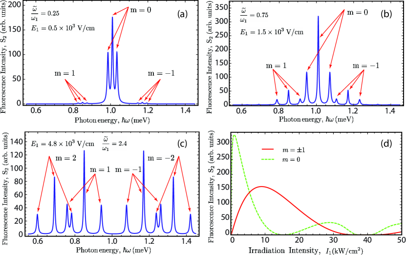
Figure 3: (Color online) The spectra of resonance fluorescence from an asymmetric quantum dot with the interlevel distance $\hbar\omega_{0}=1$ meV, dipole moments $d_{22}-d_{11}=d_{12}=40$ D, and the decay rate $\gamma=10^{-10}$ s^-1 in the presence of a bichromatic dressing field with the frequencies $\omega_{1}=0.16\,\omega_{0}$ and $\omega_{2}=0.85\,\omega_{0}$, the amplitude $E_{2}=2.2\cdot 10^{3}$ V/cm and different amplitudes $E_{1}$: (a)–(c) structure of the Mollow triplets with the numbers $m=0,\pm 1,\pm 2$; (d) Dependence of the central resonant peaks of the Mollow triplets with the numbers $m=0,\pm 1$ on the irradiation intensity $I_{1}=\varepsilon_{0}E_{1}^{2}c/4$.

In what follows, we will focus on the inelastic term (III) which is responsible for the spectral features of the resonance fluorescence.

IV Discussion and conclusion

Let us consider the effect of the two key factors of the considered system — the bichromatic structure of the dressing field and the asymmetry of the QD — on the resonance fluorescence. Mathematically, these two factors can be described by the effective frequency (12) appearing in various terms of Eq. (III). In order to explain it, we have to keep in mind that the ground and excited states of the asymmetric QD, $|1\rangle$ and $|2\rangle$, do not possess a certain spatial parity along the asymmetry axis, $z$. Therefore, the diagonal matrix elements of the dipole moment operator in an asymmetric QD prove to be nonequivalent, ${d}_{22}\neq{d}_{11}$. As a consequence, the difference of diagonal dipole matrix elements, ${d}_{22}-{d}_{11}$, describes the asymmetry of QD Kibis_09 . Since the effective frequency (12) is the product of this difference and the first field amplitude, $E_{1}$, it can be considered as a quantitative measure of both the asymmetry of the QD and the bichromatic nature of the dressing field (1). In the following, we will discuss the dependence of the resonance fluorescence on this effective frequency, $\widetilde{\omega}=(d_{22}-d_{11})E_{1}/\hbar$.

The calculated spectra of resonance fluorescence (III) are plotted in Figs. 2–3 for different effective frequencies, $\widetilde{\omega}$, near the resonance (10) with $n=1$. If the QD is symmetric or the dressing field is monochromatic ($\widetilde{\omega}=0$), the terms with $m\neq 0$ in Eq. (III) vanish since the Bessel functions of the first kind, $J_{m}\left({\widetilde{\omega}}/{\omega_{1}}\right)$, satisfy the condition $J_{m}(0)=\delta_{m0}$. The nonzero terms with $m=0$ correspond physically to the well-known Mollow triplet in the fluorescence spectrum of a two-level system driven by a monochromatic field Scully_b01 , which is plotted in Fig. 2a. If the QD is asymmetric and the dressing field is bichromatic ($\widetilde{\omega}\neq 0$), the nonzero terms with $m\neq 0$ in Eq. (III) result in the infinite set of Mollow triplets which can be numerated by the index $m=0,\pm 1,\pm 2,...$ (see Fig. 2b and Figs. 3a–3c). It is shown in Figs. 2–3 that the bichromatic dressing field generates side Mollow triplets ($m\neq 0$), shifts the main Mollow triplet ($m=0$) and change the amplitudes of the Mollow triplets. According to Eq. (III), the amplitude of the $m$-th Mollow triplet is proportional to the squared Bessel function, $J^{2}_{m}\left({\widetilde{\omega}}/{\omega_{1}}\right)$. This leads to the oscillating dependence of fluorescence peaks on the irradiation intensity, $I_{1}=\varepsilon_{0}E_{1}^{2}c/4$ (see Fig. 3d). It should be stressed that the zeros of the Bessel function, $J_{m}\left({\widetilde{\omega}}/{\omega_{1}}\right)$, correspond physically to the zero amplitude of the $m$-th Mollow triplet. Thus, the dressing field can quench fluorescence peaks. Particularly, the absence of the main Mollow triplet ($m=0$) in Fig. 3c is caused by the first zero of the Bessel function $J_{0}\left({\widetilde{\omega}}/{\omega_{1}}\right)$.

Summarizing the aforesaid, we can conclude that the exciting of asymmetric quantum systems by a bichromatic field results in the following features of resonance fluorescence spectra: an infinite set of Mollow triplets, the quench of fluorescence peaks induced by the dressing field, and the oscillating behavior of the fluorescence intensity as a function of the dressing field amplitude. To explain the physics of these novel effects, we have to stress that the considered bichromatic field (1) consists of an off-resonant dressing field $\mathbf{E}_{1}$ (which renormalizes electronic energy spectrum) and a near-resonant field $\mathbf{E}_{2}$ (which induces electron transitions between the two electronic levels). Although the dressing field $\mathbf{E}_{1}$ is off-resonant, it is very strong. Therefore, there are noticeable multiphoton processes which can involve many photons of the field. Particularly, electron transitions between the electronic levels can be accompanied by absorption of both near-resonant photon, $\hbar\omega_{2}$, and many off-resonant photons, $n\hbar\omega_{1}$, where $n$ is the number of the photons. As a consequence, there is an infinite set of resonances (10) corresponding to the different numbers $n=0,1,2,...$. Since each resonance is accompanied with its own Mollow triplet, an infinite set of Mollow triplet appears in the fluorescence spectrum. As to the field-induced quench of fluorescence peaks and the oscillating behavior of the fluorescence intensity as a function of the dressing field amplitude, these effects arise from the Bessel-function factors in Eq. (III). Physically, these factors describe the nonlinear renormalization of electronic properties with the strong dressing field $\mathbf{E}_{1}$. It should be noted that the appearance of the Bessel functions in expressions describing dressed electrons is characteristic feature of various quantum systems driven by a dressing field. Particularly, the similar Bessel-function factors describe renormalized electronic properties of dressed quantum wells Morina_15 ; Dini_16 and graphene Kibis_16 ; Kristinsson_16 .

Since the considered quantum phenomena depend on electronic parameters, the elaborated theory paves the new way to the nondestructive optical testing of various asymmetric structures. Applying the developed theory to experimental studies of asymmetric QDs, one should take into account that phonons affect strongly optical transitions in semiconductor structures. To avoid the phonon-induced destruction of the discussed fine structure of the fluorescence spectra, measurements should be performed at low temperatures, $T$, satisfying the condition $T\ll\Delta\varepsilon$, where $\Delta\varepsilon=\hbar|F_{1}|$ is the characteristic field-induced shift of electron energies (the dynamic Stark shift).

- (1) C. Cohen-Tannoudji, J. Dupont-Roc, G. Grynberg, Atom-Photon Interactions: Basic Processes and Applications (Wiley, Chichester, 1998).
- (2) M. O. Scully, M. S. Zubairy, Quantum Optics (Cambridge University Press, Cambridge, 2001).
- (3) S. H. Autler, C. H. Townes, Phys. Rev. 100, 703 (1955).
- (4) S. P. Goreslavskii, V. F. Elesin, JETP Lett. 10, 316 (1969).
- (5) Q. T. Vu, H. Haug, O. D. Mücke, T. Tritschler, M. Wegener, G. Khitrova, H. M. Gibbs, Phys. Rev. Lett. 92, 217403 (2004).
- (6) Q. T. Vu, H. Haug, Phys. Rev. B 71, 035305 (2005).
- (7) F. J. López-Rodríguez, G. G. Naumis, Phys. Rev. B 78, 201406(R) (2008).
- (8) O. V. Kibis, Phys. Rev. B 81, 165433 (2010).
- (9) O. V. Kibis, O. Kyriienko, I. A. Shelykh, Phys. Rev. B 84, 195413 (2011).
- (10) M. M. Glazov, S. D. Ganichev, Phys. Rep. 535, 101 (2014).
- (11) G. Usaj, P. M. Perez-Piskunow, L. E. F. Foa Torres, C. A. Balseiro, Phys. Rev. B 90, 115423 (2014).
- (12) A. Myzyrowicz, D. Hulin, A. Antonetti, A. Migus, W. T. Masselink, H. Morkoç, Phys. Rev. Lett. 56, 2748 (1986).
- (13) M. Wagner, H. Schneider, D. Stehr, S. Winnerl, A. M. Andrews, S. Schartner, G. Strasser, M. Helm, Phys. Rev. Lett. 105, 167401 (2010).
- (14) O. V. Kibis, Phys. Rev. B 86, 155108 (2012).
- (15) M. Teich, M. Wagner, H. Schneider, M. Helm, New J. Phys. 15, 065007 (2013).
- (16) N. Shammah, C.C. Phillips, and S. De Liberato Phys. Rev. B 89, 235309 (2014).
- (17) F. Barachati, S. De Liberato, and S. Kena-Cohen Phys. Rev. A 92, 033828 (2015).
- (18) O. V. Kibis, Phys. Rev. Lett. 107, 106802 (2011).
- (19) O. V. Kibis, O. Kyriienko, I. A. Shelykh, Phys. Rev. B 87, 245437 (2013).
- (20) F. K. Joibari, Y. M. Blanter, G. E. W. Bauer, Phys. Rev. B 90, 155301 (2014).
- (21) G. Yu. Kryuchkyan, O. Kyriienko, I. A. Shelykh, J. Phys. B 48, 025401 (2015).
- (22) J. P. Reithmaier, G. Sek, A. Löffler, C. Hofmann, S. Kuhn, S. Reitzenstein, L. V. Keldysh, V. D. Kulakovskii, T. L. Reinecker, and A. Forchel, Nature 432, 197 (2004).
- (23) T. Yoshie, A. Scherer, J. Heindrickson, G. Khitrova, H. M. Gibbs, G. Rupper, C. Ell, O. B. Shchekin, and D. G. Deppe, Nature 432, 200 (2004).
- (24) E. Peter, P. Senellart, D. Martrou, A. Lemaitre, J. Hours, J. M. Gérard, and J. Bloch, Phys. Rev. Lett. 95, 067401 (2005).
- (25) A. Muller, E. B. Flagg, P. Bianucci, X. Y. Wang, D. G. Deppe, W. Ma, J. Zhang, G. J. Salamo, M. Xiao, and C. K. Shih, Phys. Rev. Lett. 99, 187402 (2007).
- (26) S. M. Ulrich, S. Ates, S. Reitzenstein, A. Lo ffler, A. Forchel and P. Michler, Phys. Rev. Lett. 106, 247402 (2011).
- (27) A. Majumdar, M. Bajcsy, and J. Vuckovic, Phys. Rev. A 85, 041801(R) (2012).
- (28) Y. He, Y.-M. He, J. Liu, Y.-J. Wei, H. Y. Ramirez, M. Atature, C. Schneider, M. Kamp, S. Hofling, C.-Y. Lu, and J.-W. Pan, Phys. Rev. Lett. 114, 097402 (2015).
- (29) O. V. Kibis, G. Ya. Slepyan, S. A. Maksimenko, A. Hoffmann, Phys. Rev. Lett. 102, 023601 (2009).
- (30) I. G. Savenko, O. V. Kibis, I. A. Shelykh, Phys. Rev. A, 85, 053818 (2012).
- (31) F. Oster, C. H. Keitel, M. Macovei, Phys. Rev. A 85, 063814 (2012).
- (32) E. Paspalakis, J. Boviatsis, S. Baskoutas, J. App. Phys. 114, 153107 (2013).
- (33) Y. Masumoto, T. Takagahara Semiconductor Quantum Dots (Springer, Berlin, 2002).
- (34) A. Tartakovskii, Quatum Dots (Cambridge University Press, Cambridge, 2012).
- (35) F. Widmann, J. Simon, B. Daudin, G. Feuillet, J. L. Rouvière, N. T. Pelekanos, and G. Fishman, Phys. Rev. B 58, R15989 (1998).
- (36) O. Moriwaki, T. Someya, K. Tachibana, S. Ishida, and Y. Arakawa, Appl. Phys. Lett. 76, 2361 (2000).
- (37) D. P. Williams, A. D. Andreev, E. P. O Reilly, and D. A. Faux, Phys. Rev. B 72, 235318 (2005).
- (38) T. Bretagnon, P. Lefebvre, P. Valvin, R. Bardoux, T. Guillet, T. Taliercio, B. Gil, N. Grandjean, F. Semond, B. Damilano, A. Dussaigne, and J. Massies, Phys. Rev. B 73, 113304 (2006).
- (39) R. J. Warburton, C. Schulhauser, D. Haft, C. Scha flein, K. Karrai, J. M. Garcia, W. Schoenfeld, and P. M. Petroff, Phys. Rev. B 65, 113303 (2002).
- (40) I. Ostapenko, G. Honig, C. Kindel, S. Rodt, A. Strittmatter, A. Hoffmann, D. Bimberg, Appl. Phys. Lett. 97, 063103 (2010).
- (41) G. Honig, S. Rodt, G. Callsen, I. A. Ostapenko, T. Kure, A. Schliwa, C. Kindel, D. Bimberg, A. Hoffmann, S. Kako and Y. Arakawa Phys. Rev. B 88, 045309 (2013).
- (42) Z. Ficek, H. S. Freedhoff, Phys. Rev. A 53, 4275 (1996).
- (43) M. Jakob and G. Yu. Kryuchkyan, Phys. Rev. A 58, 767 (1998).
- (44) G. Yu. Kryuchkyan, M. Jakob, A. S. Sargsian, Phys. Rev. A 57, 2091 (1998).
- (45) M. Jakob and G. Yu. Kryuchkyan, Phys. Rev. A 57, 1355 (1998).
- (46) Z. Ficek, T. Rudolph, Phys. Rev. A 60, R4245 (1999).
- (47) G. A. Abovyan and G. Yu. Kryuchkyan, Phys. Rev. A 88, 033811 (2013).
- (48) H. Y. Ramirez, RSC Adv. 3, 24991 (2013).
- (49) S. N. Shevchenko, G. Oelsner, Ya. S. Greenberg, P. Macha, D. S. Karpov, M. Grajcar, U. Hübner, A. N. Omelyanchouk, E. Il ichev, Phys. Rev. B 89, 184504 (2014).
- (50) H. S. Freedhoff, M. E. Smithers, J. Phys. B 8, L209 (1975).
- (51) A. S. M. Windsor, C. Wei, S. A. Holmstrom, J. P. D. Martin, N. B. Manson, Phys. Rev. Lett. 80, 3045 (1998).
- (52) M. Macovei, M. Mishra, C. H. Keitel, Phys. Rev. A 92, 013846 (2015).
- (53) L. D. Landau, E. M. Lifshitz, Quantum Mechanics (Pergamon Press, Oxford 1965).
- (54) C. Cohen-Tannoudji, S. Reynaud, J. Phys. B 10, 345 (1977).
- (55) G. Yu. Kryuchkyan, JETP 56, 1153 (1982).
- (56) O. Kocharovskaya, S.-Y. Zhu, M. O. Scully, P. Mandel, Y. V. Radeonychev, Phys. Rev. A 49, 4928 (1994).
- (57) G. Yu. Kryuchkyan, JETP 82, 60 (1996).
- (58) S. Morina, O. V. Kibis, A. A. Pervishko, I. A. Shelykh, Phys. Rev. B 91, 155312 (2015).
- (59) K. Dini, O. V. Kibis, I. A. Shelykh, Phys. Rev. B 93, 235411 (2016).
- (60) O. V. Kibis, S. Morina, K. Dini, I. A. Shelykh, Phys. Rev. B 93, 115420 (2016).
- (61) K. Kristinsson, O. V. Kibis, S. Morina, I. A. Shelykh, Sci. Rep. 6, 20082 (2016).