Ranging with frequency-shifted feedback lasers: from $\mu$m-range accuracy to MHz-range measurement rate

Abstract

We report results on ranging based on frequency shifted feedback (FSF) lasers with two different implementations: (1) An Ytterbium-fiber system for measurements in an industrial environment with accuracy of the order of 1 $\mu$m, achievable over a distance of the order of meters with potential to reach an accuracy of better than 100 nm; (2) A semiconductor laser system for a high rate of measurements with an accuracy of 2 mm @ 1 MHz or 75 $\mu$m @ 1 kHz and a limit of the accuracy of $\geq$ 10 $\mu$m. In both implementations, the distances information is derived from a frequency measurement. The method is therefore insensitive to detrimental influence of ambient light. For the Ytterbium-fiber system a key feature is the injection of a single frequency laser, phase modulated at variable frequency $\Omega$, into the FSF-laser cavity. The frequency $\Omega_{max}$ at which the detector signal is maximal yields the distance. The semiconductor FSF laser system operates without external injection seeding. In this case the key feature is frequency counting that allows convenient choice of either accuracy or speed of measurements simply by changing the duration of the interval during which the frequency is measured by counting.

1 Introduction

Following up on earlier work in theory YAT04b ; YAT09b and experiment OGU06a ; OGU08 we report new results using the concept of ranging based on a frequency-shifted feedback laser (FSF-laser). Central to these concepts is the use of a frequency comb. Therefore our work appears fitting for this volume honoring T. Hänsch at the occasion of his 75^th birthday. However, the frequency comb used in our work is created by a cavity-internal acousto-optical frequency shifter (AOFS) and thus differs from the type of optical comb for which T. Hänsch received the Nobel Prize HAE06 . Our work is directed towards the development of systems which are suitable for industrial applications, i.e. which are accurate, robust and economic.

In Sect. 2 we present work based on a fiber-laser system aiming at high accuracy of the measurement over distances of the order of meter. An accuracy $\delta z\approx 1$ $\mu$m is documented ($\delta z/z\approx 10^{-6}$), with an expected limit of the achievable accuracy $<$ 100 nm ($\delta z/z<10^{-7}$).

In Sect. 5 we present work based on a semiconductor laser aiming at a high rate of measurements. We document the potential to achieve a measurement rate up to 1 MHz with mm accuracy. At a lower measurement rate, the accuracy of measurements with that system approaches 10 $\mu$m.

1.1 The FSF laser concept

The history of work on lasers with cavity-internal frequency shift goes back many decades, at least to the early 1970, when a Stanford group STR70 later including also T. Hänsch TAY71 showed that insertion of an AOFS into the laser cavity allowed fast wavelength tuning. That work led to the development of a new type of modelocking: Kowalski et. al. KOW87 showed that robust modelocking occurs when the AOFS frequency shift equals the free spectral range of the cavity. This was demonstrated first in a passive cavity KOW87 and later with an active cavity KOW88b ; BON96 . The group at Golden KOW88a ; HAL90 was also the first to start characterizing the optical output spectrum of a FSF laser.

The latter work triggered similar experimental and theoretical efforts in Kaiserslautern LIT91a ; LIT92 ; BAL93 ; KOW94 and later in Sendai NAK97 ; NAK98 . In parallel, the group of T. Hänsch continued to further develop the scheme as a means for tuning laser wavelength RIC91a or bandwidth control RIC91b . Aspects of the nonlinear dynamics of a FSF laser were analyzed via simulation studies in SAB94 ; STE03 ; MAR06 or in experiments MAR94 . More recent work looking at the properties of FSF lasers can be found e.g. for fiber lasers doped with Erbium VAZ13 ; VAZ14 or Thulium CHE16 , or for semiconductor lasers in NDI08 ; SEL15 .

A comprehensive general theory of the FSF-laser operation was first presented in YAT04a followed by work with special emphasis on the coherence properties of the optical output YAT09a . Further detailed analysis of FSF-laser properties and some new applications was presented by the Grenoble group CHA09 ; CHA10 ; CHA11 ; CHA13b ; PIQ13 ; CHA14 ; CHA16 .

1.2 Other applications of FSF lasers

Although our present work treats ranging based on FSF lasers, we briefly mention a few other applications of such lasers. Early work using specific properties of the FSF laser concerned the mechanical action of light on atoms, such as slowing and cooling of atoms in a beam LIT91b following up on a proposal by HOF88 or light-induced drift separation of Rb isotopes MUG93 . Further applications include accurate frequency-interval measurements BAR92 ; efficient optical pumping of atoms LIM98 ; CAS00 ; efficient excitation of atoms in the higher atmosphere for preparation of a guide star PIQ03 ; MAR07 ; PIQ11 ; observation of dark resonances in optical excitation of atoms ROM10 ; realization of a FSF laser with high BAL95 or ultrahigh and variable CHA13a pulse rate; control of pulse duration NIK09 or new schemes for frequency stabilization NIK10 ; rapid tuning of frequency LYA16 ; and generation of a frequency comb for specific tasks in underwater sensing ZHA16 .

1.3 Laser-based distance measurements

Numerous methods for laser-based distance measurement are known. Several of them are implemented in commercial devices. Here we only mention a few reviews that cover many of the well known techniques at various levels of detail AMA01 ; GRO01 ; GEN11 ; BER12a ; DEL12 . An interesting line of more recent development is based on Hänsch-type frequency combs, often with sub-mm accuracy, some of them developed for applications over very long distances in space (e.g. COD09 ; LEE10 ; BER12b ; BAU14 ; LIA14 ; JAN15 ; BER15 ; JAN16 ). One common feature of most of the techniques discussed in those reviews is the need to accurately measure, in one way or another, intensities returned from the object. Ambient light reaching the detector may therefore be detrimental to the achievement of high sensitivity or accuracy. To conclude this brief overview of past work, we mention early work WEB88 suggesting ranging based on interferometry with phase modulated light. Because this approach relies on quantitative measurement of light intensity-modulation amplitude it has not found widespread application for ranging.

1.4 Ranging based on FSF lasers

An early application of a FSF laser for distance measurement was reported by the Sendai group NAK00 using a Nd-YAG laser followed by later work ITO08 ; NDI09 including the application to the monitoring of bridge movements over 100 m range distances UME10 . A powerful modification of the FSF-ranging scheme was introduced by the Kaiserslautern group through theoretical work YAT04b followed by experimental demonstrations using lasers with an Ytterbium-doped fiber OGU06a ; OGU06b or Erbium-doped fiber OGU08 as gain medium. The theoretical frame of that work is discussed in some detail in Sect. 3. Further contributions to the scheme came from SHO06 and in particular from the Grenoble group PIQ13 . Applications using a variety of gain media, e.g. Titanium-Sapphire BRA10 and distributed feedback systems HON07a ; HON07b have also been reported.

A significant feature that sets FSF laser-based ranging technique apart from more traditional methods is the fact that the distance of an object is deduced from a frequency measurement.

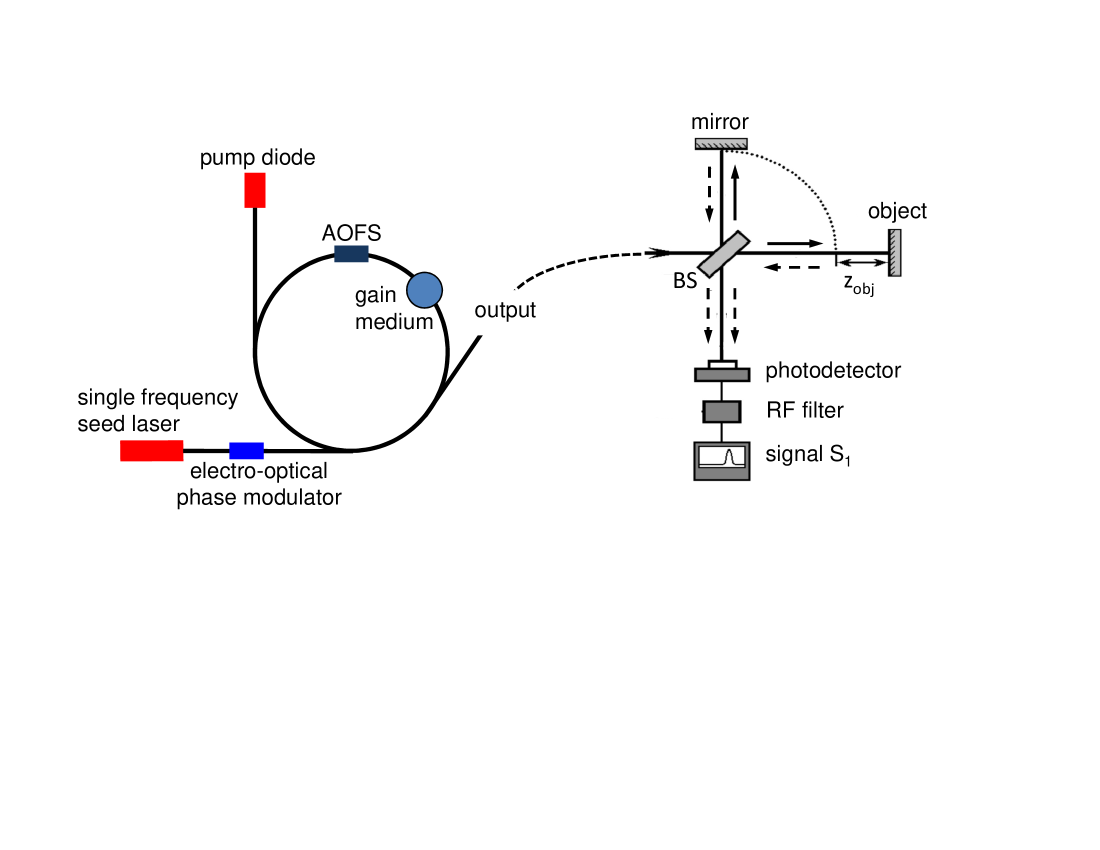
Figure 1: On the left side, the schematics of the FSF ring-laser is shown, with a Ytterbium-doped fiber as gain medium, an acousto-optical frequency-shifter AOFS, a pump diode and a single frequency ($\approx 1$ MHz bandwidth) seed laser injected into the fiber ring after passing an electro-optical phase modulator. The laser output is launched into the ranging setup, shown at the right side, with reference mirror, object, beam splitter (BS), photodetector, RF-filter and evaluation electronics. The central frequency of the RF-filter coincides with the variable frequency $\Omega(t)$ of phase modulation.

2 The fiber laser system: overview

2.1 The Ytterbium system

The characteristic elements of the FSF laser used for this experiment are shown in Fig.1. The essential components are a broadband gain medium (here a Yb³⁺-doped optical fiber), an intracavity acousto-optical frequency shifting element (AOFS), a pump laser (diode laser) and an output port. The AOFS is inserted into the ring via fiber pigtails adjusted such that only the frequency-shifted first diffraction order of the AOFS is allowed to continue circulating in the ring cavity. A specific and crucial feature of this setup is a single-frequency CW laser, the radiation of which is injected into the ring cavity after passing through an electro-optical phase modulator BER03 .

The radiation reflected from the reference surface and the time-delayed comb scattered from the object are superimposed on the detector leading to a multi-component signal, see Eqs. (8) and (9) below. The follow-up electronics looks at the amplitude of the ac-component of the signal at frequency $\Omega$. The modulation frequency $\Omega_{0}$ at which this signal is maximal, yields – according to Eq. (13) below – directly the distance to the object. Thus, a measurement proceeds by tuning the modulation frequency $\Omega$ over a suitable frequency range. During the scan the frequency $\Omega_{0}$ is determined.

Ranging with an accuracy of the order of 1 $\mu$m requires a broad optical spectrum which can be realized by e.g. a fiber laser system as used in this experiment. Yb³⁺-doped optical fibers have a large gain bandwidth due to strongly broadened laser transitions in glasses. Ytterbium ions Yb³⁺ have a simple electronic level structure, with only one excited state manifold (²F_5/2) which can be exited from the ground-state manifold (²F_7/2) with near-infrared radiation. The level scheme has a quasi-three-level character. Compared to the semiconductor gain medium (see Sect. 5) Yb³⁺-doped fiber gain has a much larger saturation intensity and longer upper-state lifetime (typically of the order of 1–2 ms).

All components are spliced together leaving no adjustable elements. Figure 1 shows also the schematics of the Michelson arrangement implemented for detecting the ranging signal. An extra mirror for the reference path may not be needed if the reflection from the end facet of the fiber, which delivers the radiation to the object, serves as reference beam.

2.2 Comparison with FMCW-Ladar

At first glance the FSF-laser ranging concept appears similar to the frequency-modulated scheme for laser detection and ranging (FMCW-Ladar, see e.g. BER12a ; DIE94 ; MAT15 ), a technique which allows measuring a beat frequency resulting from single-frequency laser radiation, the frequency of which is linearly changed in time with a chirp rate $\gamma_{c}$ periodically repeated in a saw-tooth pattern. That radiation is sent via a beam splitter to a reference surface and the object before being recombined at the detector. Any difference $z_{obj}$ in path length to the reference mirror and the object results in a beat frequency $\Omega_{beat}$ from which $z_{obj}$ is deduced according to

$$z_{obj}=\frac{c}{2}\frac{\Omega_{beat}}{\gamma_{c}}.$$ (1)

Obviously for high accuracy a large $\Omega_{beat}$ and thus a large $\gamma_{c}$ (a steep chirp) is wanted. Furthermore, high accuracy requires a strictly linear variation of frequency with time.

However, the physics underlying the generation of a ranging signal by a FSF laser differs from the physics of FMCW-Ladar, see Sect. 3.

3 Theoretical background

3.1 The FSF-laser field

Following YAT04a the output field ${E}(t)$ of the FSF laser, seeded by laser radiation of amplitude $\mathcal{E}_{0}$, frequency $\omega_{s}$ and phase $\varphi_{s}(t)$, is a sum of many discrete components

$${E}(t)=\sum_{n=0}^{\infty}\mathcal{E}_{n}\exp[-i(\omega_{s}+n\Delta)t-i\Phi_{n}-i\varphi_{s}(t-n\tau)],$$ (2)

because the seed laser is strong enough to dominate over any seeding by spontaneous emission within the gain medium. The frequency of component $n$ is shifted from $\omega_{s}$ by $n\Delta$ where $\Delta$ is the AOFS-induced frequency shift per round trip. The phase of this component is given by the phase $\varphi_{s}$ of the seed laser taken at the time $t_{0}=t-n\tau$ (which is the time when the radiation relevant for this component entered the cavity), augmented by the additional phase shift $\Phi_{n}$ due to the propagation within the cavity,

$$\Phi_{n}=-n\tau[\omega_{s}+(n+1)\Delta/2],$$ (3)

where $\tau$ is the cavity round-trip of the FSF laser. Saturated gain from the amplifying medium and loss from any spectral filter that may act in the cavity alter the original seed amplitude $\mathcal{E}_{0}$ to the values $\mathcal{E}_{n}$. The distribution of amplitudes $\mathcal{E}_{n}$ of the discrete spectral components is well described YAT04a by a Gaussian

$$\mathcal{E}_{n}=\mathcal{E}_{0}\exp\left[-\frac{(n-n_{max})^{2}}{n_{W}^{2}}\right].$$ (4)

centered at the component $n_{max}$ where the intensity reaches its maximum. The parameter $\Delta n_{max}$ is the shift of the maximum of the optical spectrum of the FSF laser from the frequency of the seed laser. The parameter $n_{W}$ is the width of the Gaussian distribution of amplitudes $\mathcal{E}_{n}$. Accordingly, the width of the optical spectrum is determined by the distribution of intensities $\propto|\mathcal{E}_{n}|^{2}$ and is equal to $\Delta n_{W}/\sqrt{2}$. Typically we have $n_{max}\sim n_{W}$ and $10^{3}<n_{W}<10^{4}$.

The phase of the seed laser is periodically changed by an electro-optical modulator (EOM) according to

$$\varphi_{s}(t)=\beta\sin(\Omega t+\vartheta),$$ (5)

where $\Omega$ is the modulation frequency, $\beta$ the modulation index and $\vartheta$ an (irrelevant) initial phase. The frequency $\Omega$ of this phase modulation is a crucial parameter in the experiment.

3.2 The structure of the ranging signal

The fields returned from the reference surface and from the object are combined at the detector. The signal delivered by the detector depends on $t$, $\Omega$ and $T$, where $T$ is the delay of the time of arrival of radiation coming from the reference surface and from the object. The signal is evaluated from

$$S(t;\Omega,T)=\left\langle\left|{E}(t;\Omega)+E(t-T;\Omega)\right|^{2}\right\rangle,$$ (6)

where $\left\langle\,\,\right\rangle$ means averaging over a period long compared to the optical cycle $\omega_{s}^{-1}$ but short compared with the modulation cycle $\Omega^{-1}$.

The signal $S(t;\Omega,T)$ is a superposition of many harmonics of the modulation frequency YAT04b

$$S(t;\Omega,T)=\sum_{l}S_{l}(\Omega,T)\exp(il\Omega t).$$ (7)

We use an electronic filter to restrict detection of the signal at the modulation frequency $\Omega$ yielding $S_{1}(\Omega,T)$. Using Eqs. (2), (3), (5), and (7) we obtain

$$S_{1}(\Omega,T)=J_{1}(X)\sum_{n}|\mathcal{E}_{n}|^{2}\left[P_{n}^{-}-P_{n}^{+}\right]$$ (8)

with

$$P_{n}^{(\pm)}=\exp\{-i[n(\Omega\tau\pm T\Delta)-\psi]\}.$$ (9)

Here $J_{1}(X)$ is a Bessel function and $X=2\beta\sin(\Omega T/2)$. The phase

$$\psi=\omega_{s}T-(\Omega T+\pi)/2+\theta$$ (10)

does not depend on $n$. The term $n\Omega\tau$ originates from the propagation within the FSF cavity and $nT\Delta$ results from the accumulated AOFS-induced shift of the optical frequency of the $n$-th component of the field, Eq. (2).

In the experiment the signal $|S_{1}(\Omega,T)|$ is measured as a function of $\Omega$. For each $n$ we have two contributions to $S_{1}(\Omega,T)$ with amplitude according to Eq. (4). The phase factors $P_{n}^{(\pm)}$, Eq. (9), depend on $n$, the system parameters $\tau$ and $\Delta$ and the variables $\Omega$ and $T$. As $n$ increases from $n=1$ to $n>n_{max}$ ($n_{max}\approx 10^{4}$) the phases $n(\Omega\tau\pm T\Delta)-\psi$ of $P_{n}^{(\pm)}$ will go, for given $\Omega$ and $T$, through very many cycles of $2\pi$ and thus their contribution to $|S_{1}(\Omega,T)|$ will be small unless we have either $\Omega\tau-T\Delta=2\pi m$ or $\Omega\tau+T\Delta=2\pi k$ with integer $m$ and $k$. In that case the phases of either the first term, associated with $P_{n}^{-}$, or the second term, associated with $P_{n}^{+}$, will be equal to $2\pi mn-\psi$ or $2\pi kn-\psi$, respectively, meaning that $P_{n}^{-}$ or $P_{n}^{+}$ is in effect independent of $n$.

Assuming $T>0$ (as in our experiment) we realize that for the modulation frequency $\Omega=\Omega_{q}^{+}$ given by

$$\Omega_{q}^{+}=\gamma_{c}T+q\Delta_{FSR};\quad q=-M_{0},-M_{0}+1,\ldots$$ (11)

the terms of Eq. (8) associated with $P_{n}^{+}$ tend to sum up to a very small value, if not zero. However, the coefficients $P_{n}^{-}$ are independent of $n$ and the sum reaches a possibly large absolute value $S_{max}$. In Eq. (11) $\gamma_{c}=\Delta/\tau$ is the chirp rate in the moving comb model of FSF laser YAT04a ; KAS98 , and $M_{0}$ is the integer part of $T\Delta/2\pi$. Similarly, for the modulation frequency $\Omega=\Omega_{p}^{-}$ given by

$$\Omega_{p}^{-}=-\gamma_{c}T+p\Delta_{FSR};\quad p=M_{0}+1,M_{0}+2,\ldots$$ (12)

the terms of Eq. (8) associated with $P_{n}^{-}$ tend to sum up to a very small value. In this case, the coefficients $P_{n}^{+}$ are independent of $n$ and the absolute value of the sum reaches the same large value $S_{max}$.

The electronics for the data analysis tracks the detector signal $|S_{1}(\Omega,T)|$, for a given $T=2z_{obj}/c$. Here $z_{obj}=0$ marks the location of the end of the fiber, where the reference laser beam and the beam sent to the object are separated. In the present experiment this is the end facet of the optical fiber which launches the laser beam towards the object. The modulation frequency $\Omega_{max}$ at which $|S_{1}(\Omega,T)|$ reaches its maximum is recorded. For a short distance $T<2\pi/\Delta$ (meaning $M_{0}=0$), as is typical for our experiment, the first two frequency $\Omega_{max}$ are $\Omega_{0}^{+}=\gamma_{c}T$ and $\Omega_{1}^{-}=-\gamma_{c}T+\Delta_{FSR}$. We can use both of these frequencies to find the distance $z_{obj}$. In the present experiment we use the resonance at $\Omega_{0}^{+}=\gamma_{c}T$ and find the distance $z_{obj}$ from

$$z_{obj}=\frac{c}{2}\frac{\Omega_{0}^{+}}{\gamma_{c}}.$$ (13)

When the measurement aims at an accuracy of 1 $\mu$m the order $q$ or $p$ will usually be known. When this is not the case the ambiguity can be resolved experimentally, see Sect. 5.

In case of a smooth dependence of the amplitudes $\mathcal{E}_{n}$ on $n$ the function $S_{1}(\Omega,T)$, Eq. (8), represents the Fourier transform of the optical spectrum of the FSF laser. For a Gaussian optical spectrum, Eq. (4), the variation of the $|S_{1}(\Omega,T)|$ with $\delta\Omega=\Omega-\Omega_{max}$ is also Gaussian:

$$|S_{1}(\Omega,T)|=S_{max}\exp\left\{-\left[\frac{\delta\Omega^{2}}{\delta\Omega_{0}^{2}}\right]\right\},$$ (14)

where

$$\delta\Omega_{0}=\frac{2\sqrt{2}}{n_{W}\tau}.$$ (15)

The method is not sensitive to detrimental influence of ambient light or to a variation of the intensity of the light returned from the object, as long as $|S_{1}(\Omega,T)|$ is large enough to reliably determine $\Omega_{max}$.

Furthermore the accuracy $\delta z$ of a measurement is determined by the width $\delta\Omega_{0}$ of $|S_{1}(\Omega,T)|$. The accuracy $\delta\Omega_{max}$ of a measurement of $\Omega_{max}$ is $\delta\Omega_{max}=\epsilon\delta\Omega_{0}$ where $\epsilon$ is determined by the electronic recording system and laser noise. In our experiment we typically have $10^{-3}<\epsilon<10^{-2}$. According to Eqs. (4), (13) and (15), the uncertainty of $\Omega_{max}$ leads to uncertainty $\delta z$ of distance

$$\delta z=\epsilon\frac{2c}{\Gamma_{opt}},$$ (16)

where $\Gamma_{opt}=n_{w}\Delta/\sqrt{2}$ is the width of the optical spectrum of the FSF laser. Thus the attainable accuracy of the distance measurements is given exclusively by the width of the optical spectrum and does not depend on distance. Furthermore, because the signal $S_{1}(\Omega,T)$ is caused by beating the radiation which propagates along the reference path ($I_{ref}$) and the path to the object ($I_{obj}$), its amplitude is $\propto\sqrt{I_{ref}I_{obj}}$ and thus varies with $z_{obj}$ as $1/z_{obj}$ rather than as $1/z_{obj}^{2}$.

4 Experiment

4.1 The fiber FSF laser

The all-fiber Yb³⁺-doped FSF ring laser (schematically shown in Fig. 1) with a free-spectral range $\Delta_{FSR}=113,6$ MHz ($\tau=8.8$ ns) is a compact transportable system similar to the one used in refs. OGU06a , OGU08 , and OGU06b . The gain medium of the laser is a 40 cm long Yb³⁺-doped active fiber pumped by a diode laser ($\lambda=976$ nm, $P=300$ mW) which is coupled into the ring via a wavelength division multiplexer (WDM). The intra-cavity fiber-pigtail acousto-optic frequency shifter increases the frequency of the radiation circulating in the cavity by 200 MHz per round trip, leading to a ”chirp rate” of $\gamma_{c}=\Delta/\tau=2.3\cdot 10^{16}$ Hz/s. The single frequency seed laser is a diode laser in Littmann-Metcalf configuration LIT78 ; LIU81 . The voltage driving the EOM phase modulator is generated by a digital synthesizer.

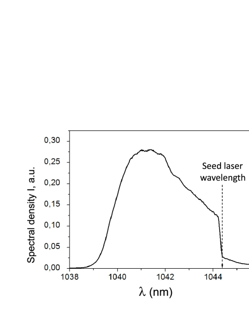
Figure 2: The spectum of the FSF-laser radiation recorded with low resolution. The comb structure is not resolved. The seed-laser frequency is marked. The AOFS shift is to higher frequencies.

Figure 2 shows a typical spectrum of the FSF-laser radiation with its central wavelength near $\lambda_{c}=1041$ nm and width of 5 nm. Experiments are typically done with an output power of $P=10$ mW. Fiber couplers are used to inject the seed laser into the cavity and to couple radiation out of the cavity. All fiber components are connected by fusion splices.

4.2 The detection system

The modulation frequency $\Omega(t)$ is linearly scanned across an interval $\Delta\Omega$ which includes the resonance frequency according to Eq. (11) or Eq. (12). Typically $\Delta\Omega$ is set to cover a range of changes of $z_{obj}$ less than 2 mm. The FSF-laser radiation is sent via fibers through a circulator before being launched towards the object. The reference beam is either generated by the reflection off the end facet of the fiber, see Fig. 3, or in a Michelson interferometer setup, see Fig. 1.

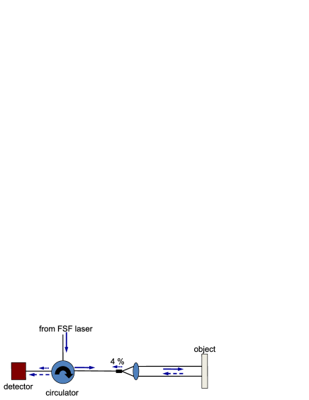
Figure 3: Details of the Michelson interferometer setup. The circulator directs the radiation from the FSF laser via a fiber to the object. The light reflected from the end facet of the fiber serves as the reference beam. The reflected beams are directed by the circulator to the detector.

The returning radiation is coupled into the same fiber, reaches the circulator again and is directed by it to the fast InGaAs photodetector of area 0.2 mm² with fixed gain, a bandwidth of 150 MHz and a sensitivity range of 800–1700 nm. The detector signal passes an electronically controlled bandpass filter with a high transmission in the vicinity of the modulation frequency $\Omega$ before being sent to the evaluation electronics which records the modulation frequency $\Omega_{max}$ at which the signal $|S_{1}(\Omega,T)|$ reaches its maximum. An automatic level-control assures that the evaluation electronics processes a signal of about the same magnitude, within limits independent of the intensity of the light returned from the object.

4.3 Results

4.3.1 Accuracy

The data shown in Fig. 4 are taken with the FSF-laser radiation launched towards the object via a telescope (Fig. 4a)

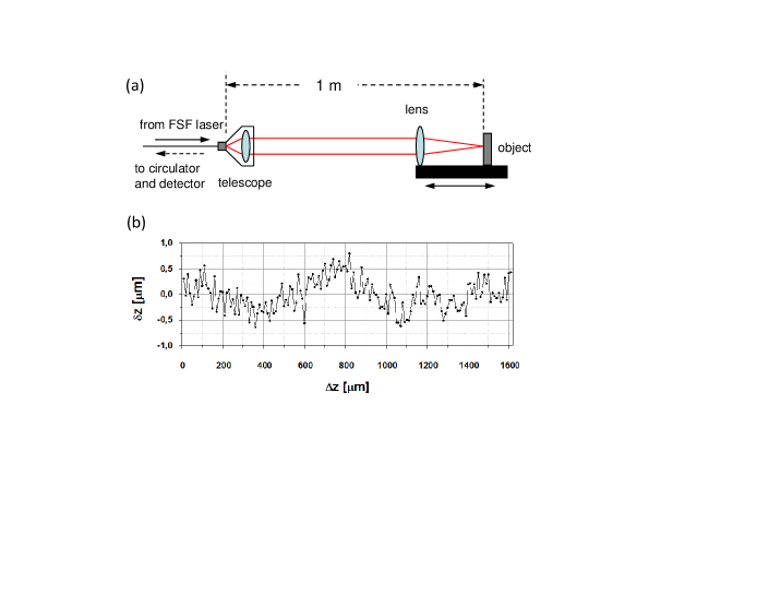
Figure 4: Accuracy of the FSF laser based measurement. (a) Optical setup. The object and the focusing lens are jointly mounted on a platform. The position of the platform is varied under the control of a linear encoder with better than 100 nm accuracy. (b) Deviation $\delta z$ of the result provided by the linear encoder and by the FSF laser based measurement while the position of the platform is changed over a range of $\Delta z_{max}=1.6$ mm. The position $\Delta z=0$ corresponds to $z_{obj}=1002,139$ mm, known from the frequency measurement to an accuracy of 1 $\mu$m.

which expands the beam diameter to 8 mm before it is focused to a 15 $\mu$m spot onto the surface. For testing the accuracy of the system, the object and the focusing lens are both mounted on a platform which is moved to change the distance $z_{obj}$. Thus, the size of the laser spot on the object does not change when $z_{obj}$ is varied. The variation of the position $z_{obj}$ of the platform, and thus the position of the object, is independently monitored with a Heidenhain linear encoder with an accuracy of better than 100 nm. An Abbe error may arise from an angular deviation $\theta$ of the direction along which the platform motion is measured from the direction of propagation and the laser beam. Therefore the angle $\theta$ was kept below 0.1 degrees. In this case the Abbe error does not exceed 10 nm.

The accuracy of the laser-ranging result is documented in Fig. 4b with the object placed at $z_{obj}\approx 1$ m (the exact reading from the frequency measurement for $\Delta z=0$ is $z_{obj}=1002,129$ mm accurate to 1 $\mu$m) and moved in steps of 10 $\mu$m over the distance $\Delta z=1.6$ mm while the variation of the position is measured through both the FSF-laser system and the linear decoder. Figure 4b shows the deviation $\delta z$ of these two readings. Each point is an average over one hundred measurements, each of 2 ms duration. The deviation $\delta z$ of the results of the laser measurement from the result of the linear encoder is $\delta z\leq 0.8$ $\mu$m ($\delta z/z<10^{-6}$). The apparently periodic deviation from $\delta z=0$ by no more than 0.6 $\mu$m is caused by diffraction on the focusing lens which can shift $\Omega_{max}$ from the value given by Eq. (11). An analysis [Yatsenko and Bergmann, to be published] shows that under uncontrolled conditions (nonideal focusing, titled object, non-Gaussian FSF laser spectrum) this deviation may reach the order of $\mu$m.

Further characterization of the system is documented in Fig. 5. Here the distribution of results from 10³ sweeps of $\Omega$ across the bandwidth $\Delta\Omega$ are shown for a fixed distance $z_{obj}=1002,627$ mm. The distribution is characterized by a standard deviation of $\sigma=1.1$ $\mu$m. We emphasize that the width of the distribution is independent on the distance $z_{obj}$ to the object. The accuracy of a single measurement, taken during a 2 ms sweep of $\Omega$, is $3\sigma\approx 3$ $\mu$m. If time is available for e.g. a thousand measurements (in a total of a few seconds) the maximum of the distribution, like the one shown in Fig. 5, can easily be determined to less than 10% of its width corresponding to an uncertainty of 100 nm or less. The accuracy of the measurements is determined by the width of the resonance (see Eq. (16)). Like most other absolute ranging methods the FSF laser ranging technique determines the optical path length between the laser and the object. Therefore, for larger distances, the variation of the refractive index along the path during the measurement could be important. Due to air turbulence, variation of the temperature profile etc. the air refractive index will deviate from the value $(n_{air}-1)10^{8}=27403.6$ EDL66 . According to JAN16 the relative uncertainty of the distance can be estimated to be about $\delta z_{obj}/z_{obj}=2\cdot 10^{-8}$. For our experimental conditions the influence of the uncertainty of $n_{air}$ needs to be considered only for $z_{obj}>5$ m.

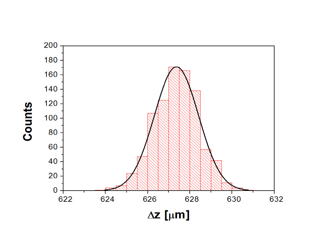
Figure 5: Distribution of the result of 10³ FSF laser based measurements taken at a fixed position near $\Delta z=627$ $\mu$m, see Fig. 4. A Gaussian fit leads for this distribution to the standard deviation of $\sigma=1.1$ $\mu$m.

4.3.2 Ambiguity

Like in any modulation-based ranging system, FSF-ranging exhibits ambiguity regarding the results. A measured distance is known only modulo the addition of a multiple of the unambiguity range, which – for our Ytterbium system – is of the order of 1 m. The latter range is determined exclusively by the size of the AOFS frequency shift. However, being interested in micron-range accuracy the prior uncertainty is usually much less than the ambiguity range. Should that not be the case, the procedure discussed in Sec. 5.2 is applicable.

4.3.3 Scanning object surfaces

A series of experiments was conducted to demonstrate the high quality of surface topography recording. In this case, the focusing lens, shown in Fig. 4a, is not attached to the table. The scanning of the object in the $x-y$-plane is done with stepper motors in increments of 10 $\mu$m. The variation of the position is monitored by linear encoders of the type mentioned above. The coordinate $z$ is measured through the FSF laser ranging method. The surface topography is reconstructed from the measured coordinates ($x,y,z$).

Figure 6 shows a step of 110 $\mu$m in an otherwise flat blackened-metal surface positioned at a distance of $z_{obj}\simeq 1$ m. The surface normal is not oriented exactly parallel to the direction of the incident laser beam axis. The average amplitude of the wiggles marking the boundary between colors is consistent with the accuracy of the order of 1 $\mu$m, as documented in Figs. 4 and 5.

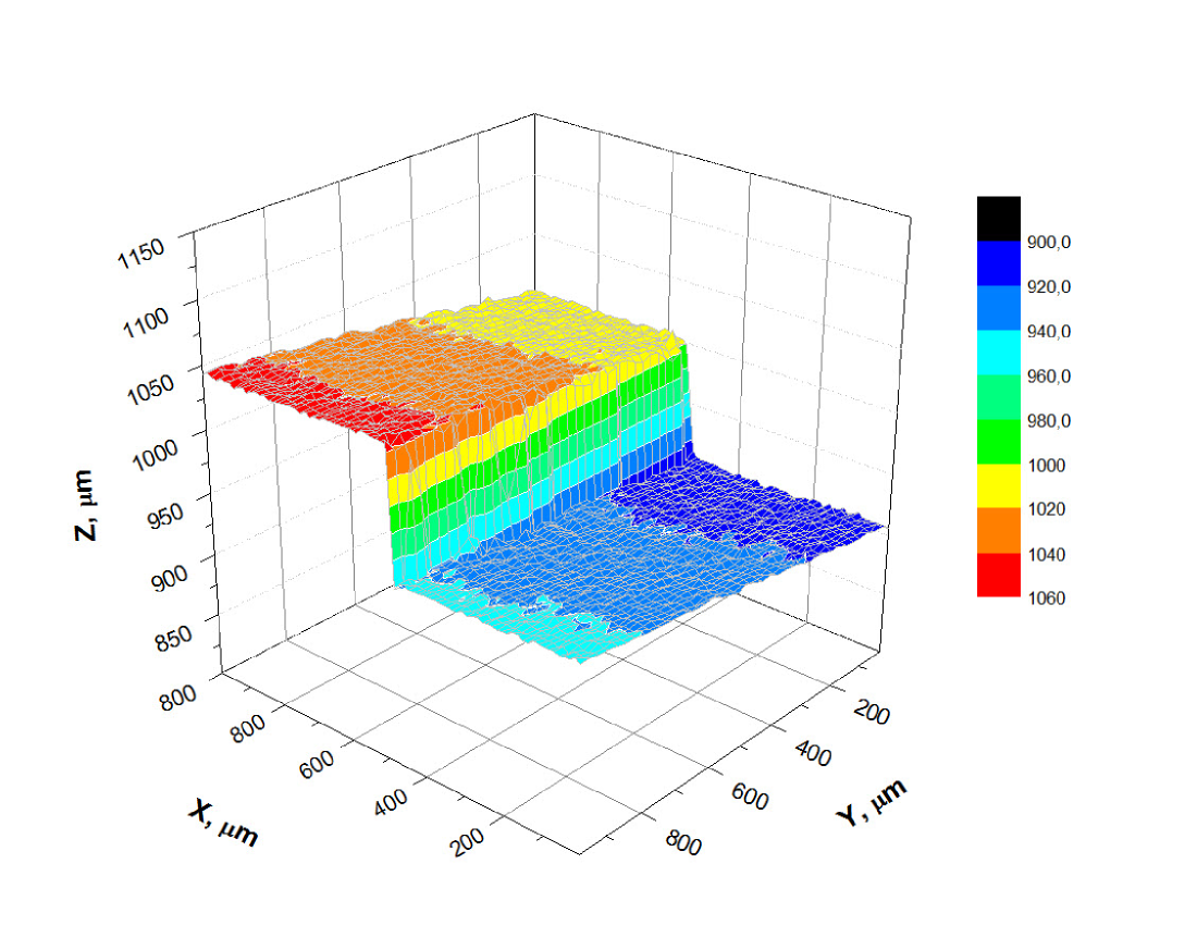
Figure 6: False colour representation of the topography of a flat black unpolished metal surface with a 110 $\mu$m step, taken from a distance of 1 m. The surface normal was not exactly parallel to the axis of the laser beam. The step size in the $x$- and $y$-direction was 10 $\mu$m. The diameter of the laser spot on the surface was 15 $\mu$m.

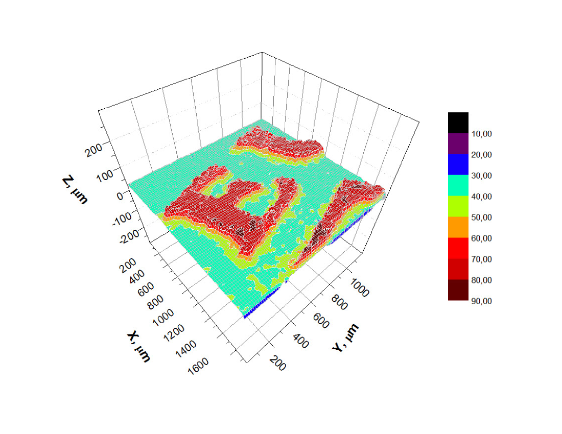
Figure 7: False colour representation of the surface topography of a segment from a Euro 2-cent coin taken from a distance of 1 m. The experimental conditions are the same as for Fig. 6.

Figure 7 shows the surface topography of the letter ”E” of a Euro 2-cent coin (see Fig. 8) also taken from a distance of $z_{obj}\simeq 1$ m. Figure 8 shows the same letter ”E”, now using the full information content of the data set (see Fig. 7), after rendering, together with a photo of the coin. The high potential of our approach may be best appreciated by comparison with AFL15 , which shows the topography of an US one-cent coin recorded with a $4\times 4$ array of detectors, using a time-domain frequency modulated continuous wave ranging scheme.

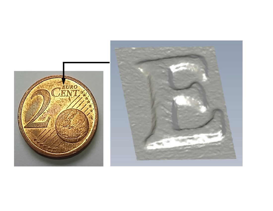
Figure 8: The right frame shows the region of a Euro 2-cent coin (see left frame) near the letter E as recorded by FSF laser ranging at a distance of 1 m after rendering, based on the same set of data used for Fig. 7.

5 The semiconductor-laser system

Many applications are anticipated (e.g. documentation of objects of meter-size or larger) where speed of measurement, rather than the highest possible accuracy is important. The minimum duration $\Delta t_{min}$ of a measurement of the kind described in the previous section for a fiber-laser system is set by the width of the RF resonance. Recalling (see Eq. (4)) that $n_{W}=\sqrt{2}\Gamma_{opt}/\Delta$, we find from Eq. (15) with $\Delta t_{min}=1/\delta\Omega_{0}$

$$\Delta t_{min}=\frac{\Gamma_{opt}}{2\Delta}\tau.$$ (17)

Thus, for high speed measurements it is preferable to work with a smaller optical bandwidth, a large $\Delta$ and in particular a short cavity. The lower limit for the length of the cavity is given by the size of the AOFS and the dimensions of the gain medium. When a semiconductor gain medium is used the size of the cavity can be much smaller compared to a system based on a doped fiber. In fact we have $\tau=0.8$ ns ($\Delta_{FSR}=1.3$ GHz) for the system discussed below.

However, some properties of a semiconductor gain medium differ distinctly from those of doped fibers. For instance, the upper state lifetime in a semiconductor system is orders of magnitudes shorter than in a fiber system and the rate of spontaneous emission is accordingly larger. It is therefore difficult, if not impossible, to control the emission spectrum of the FSF laser towards yielding a single frequency comb by injecting a narrow band laser as successfully done for the fiber system. As a consequence, we do not expect for a semiconductor gain medium the optical spectrum of the FSF laser to consist of a well-defined frequency comb with isolated frequency components separated by $\Delta$. Rather, each photon spontaneously emitted into a cavity mode will be amplified in successive round trips and create a comb with frequency components separated by $\Delta$. Because the spontaneous emission processes occur throughout the spectral profile the superposition of all the frequency combs started by individual emission processes will lead to a continuum spectrum with no immediately obvious comb structure.

5.1 Theoretical background

Without external seed laser, the output of the FSF laser is dominated by spontaneous emission processes within the gain medium. These processes are uncorrelated and intrinsically incoherent. However, the fourth-order correlation-function analysis YAT09a , which allows the evaluation of the RF spectrum of the output intensity of a Michelson interferometer, shows that this spectrum comprises a set of doublets, whose frequencies are given by Eqs. (11) and (12). This structure in the RF spectrum of a Michelson-interferometer output results from the correlation of interference terms of individual components of a cyclostationary stochastic process YAT09a . The spectrum carries information about the path length difference of the interferometer arms (the distance to be measured) and was used in early work for ranging NAK00 . Of interest is the frequency for which the spectral density of the fluctuation reaches a maximum. This approach is similar to the one described for the fiber system in Sect. 2 but is less accurate because the origin of the resonance is noise YAT04a .

Another option, used here, for accessing the information about distance is the direct frequency counting of the quasi-monochromatic output of the RF filter. This approach requires the isolation of only a single resonance in the RF spectrum of the interferometer output (see. Sect. 5.2). This approach allows a convenient choice of either speed or precision of the measurement by simply choosing an appropriate duration of the gate during which the frequency is determined by counting oscillation periods.

The interferometer output intensity filtered near one of the frequencies given by Eq. (11) or Eq. (12) is the quasi-monochromatic signal

$$I(t)=\delta I(t)\cos[\Omega_{max}t+\phi(t)].$$ (18)

Here $\delta I(t)$ and $\phi(t)$ are slow random function of time with autocorrelation time $1/\delta\Omega_{0}$ where $\delta\Omega_{0}$ is the RF resonance width given by Eq. (15). Theoretical analysis [Yatsenko and Bergmann, to be published] shows that the mean value $\delta I_{0}=\sqrt{\langle\delta I^{2}(t)\rangle}$ of the amplitude of the oscillating part of the interferometer output depends on the width $\Gamma_{opt}$ of the optical spectrum of the FSF laser and is given by

$$\delta I_{0}=2\sqrt{(1-R)R}|r|\frac{(2\pi)^{1/4}}{\sqrt{\Gamma_{opt}\tau}}I_{0}.$$ (19)

Here $R$ is the ratio of the power sent to the reference mirror and the object surface, the coefficient $r$ describes the efficiency of the collection system efficiency, $I_{0}$ is the mean output intensity of the FSF laser. The amplitude $\delta I_{0}$ can be quite large especially for the semiconductor gain medium used for our experiment in combination with a short cavity length. For example, for $R=1/2$, $r=1$ (which is the case for a highly reflecting surface), $\Gamma_{opt}=200$ GHz, $\tau=1$ ns we have $\delta I_{0}\simeq 0.045I_{0}$ which can be conveniently recorded and evaluated.

However, the noise origin of the oscillatory signal leads to a challenge in the practical implementation of the scheme. Figure 9 shows a simulated realization of the process, Eq. (18), for a Gaussian spectrum with width $\Gamma=0.1\Omega_{max}$ and an experimental trace of the oscillating component of the linear-cavity FSF-laser output described in Sect. 5.3. The fluctuation of the amplitude does not prevent the frequency counting except when the signal amplitude is close to zero, as occurs at random times. The short period, during which the amplitude falls below a threshold needed for the counting must be excluded by electronic means to obtain the highest possible accuracy.

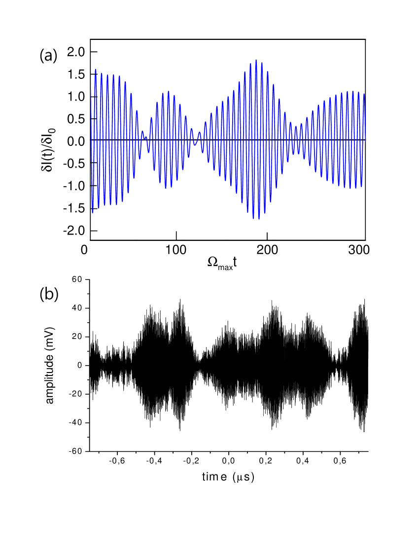
Figure 9: (a) A simulated realization of the noise process, Eq. (18), for a Gaussian spectrum of width $\Gamma=0.1\Omega_{max}$. (b) Experimental trace of the oscillating component of the linear-cavity FSF-laser output (see Sect. 5.3).

5.2 Elimination of ambiguity

Interferometric measurements determine the distance only to within an integer multiple of an unambiguity distance $z_{ua}$ OGU08 . Procedures which allow resolving the ambiguity of the detector reading are well known. The measures required in our case needs a discussion of the RF spectrum of the detector signal.

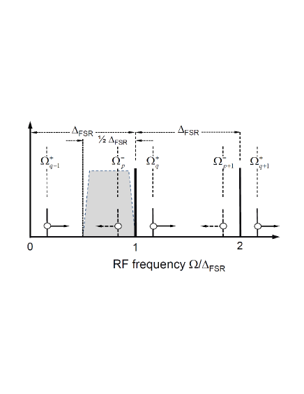
Figure 10: The RF spectrum recorded by the detector. The frequency range to be selected for detection and frequency counting is marked by the trapezoidal shaded area. The arrows attached to the short dashed or solid lines indicate the direction of change of their frequency when $z_{obj}$ and thus $\gamma_{c}T$ increase.

Because any fluctuation of the laser intensity is likely to experience some recurrence after one round trip of the radiation in the cavity, the RF spectrum of the output of the FSF laser may show a set of spectral components which are separated in frequency by the free-spectral range $\Delta_{FSR}$ of the cavity. Such components separated by $\Delta_{FSR}$ are schematically shown as long thick vertical lines in Fig. 10.

When the distance of the object, and thus $\gamma_{c}T$, increases the spectral components shown as short vertical dashed lines in Fig. 10 decrease in frequency while the frequency of the other components shown as short vertical solid lines in Fig. 10 increase. Each one of these components carries the information about $\gamma_{c}T$. The structure shown in Fig. 10 is repeated within neighboring frequency intervals of bandwidth $\Delta_{FSR}$. The following discussion deals only with one of the spectral regions, for instance with the one including the RF components in the range $0<\Omega/\Delta_{FRS}<1$. Electronic filters assure that spectral components outside this spectral range are not detected. In the case shown it happens that $\Omega^{+}_{q-1}<\Omega^{-}_{p}$. However, depending on the value of $\gamma_{c}T$, we could also have $\Omega^{+}_{q-1}>\Omega^{-}_{p}$. The frequencies of these two components are symmetric about the middle of the given spectral range. For frequency counting to successfully determine $T$ (and thus the distance $z_{obj}$) only one single spectral component is allowed in the spectral range in which the detector plus subsequent electronics has nonzero sensitivity. In order to avoid low frequency noise it is best to use an electronic filter which restricts detection to the higher-frequency part of width $\Delta_{FSR}/2$, shown in Fig. 10 as shaded area.

We will now discuss the straight forward procedure for (i) the determination of the order $p$ or $q$, resolving the ambiguity issue and (ii) how to deal with the situation when $\gamma T\approx M\Delta_{FSR}/2$ ($M$ is an integer number), i.e. when the spectral components $\Omega^{+}_{q-1}$ or $\Omega^{-}_{p}$ fall near the edge of the sensitive range set by the electronic filter. The latter (problematic) situation is easily overcome by installing a second reference path. The light returned from this additional reference surface is superimposed with a fraction of the light returned from the object on a second detector. The length of the second reference path is adjusted such that the spectral components are shifted by about an odd integer of $\Delta_{FSR}/2$. With this arrangement, there is always one detector for which the relevant spectral feature is not close the edge of the filtered bandwidth.

The determination of the order $p$ or $q$ is easily done by repeating a given measurement with a slightly different AOFS frequency $\Delta$. From Eq. (11) and recalling that $\gamma_{c}=\Delta/\tau$ we determine the variation $\delta\Omega^{\pm}$ of $\Omega^{\pm}$ when the frequency shift $\Delta$ is changed by $\delta\Delta$ and arrive for $\Omega^{+}$ at

$$q=\frac{\Omega^{+}}{\Delta_{FSR}}\left(1+\frac{\Delta}{\Omega^{+}}\frac{\delta\Omega^{+}}{\delta\Delta}\right),$$ (20)

and accordingly for $\Omega^{-}$ and the order p, starting from Eq. (12). Because $\Delta$ and $\Delta_{FSR}$ are known, measuring $\Omega^{\pm}$ and $\delta\Omega^{\pm}/\delta\Delta$ will lead to the value of the wanted order. Experiments have confirmed that a variation of $\delta\Delta/\Delta\leq 10^{-3}$ suffices to reliably determine the order $p$ or $q$. The sign of $\delta\Omega^{\pm}/\delta\Delta$ will reveal whether we detect a component of type $\Omega^{+}$ or $\Omega^{-}$.

We conclude this discussing by determining the unambiguity range $z_{ua}$ for our experimental conditions. As discussed above the determination of $z_{obj}$ is unambigious when $\Omega=\gamma_{c}T\leq\Delta_{FSR}/2$, what leads with $T=2z_{obj}/c$ to

$$z_{ua}=\frac{c}{4\Delta}.$$ (21)

We also note an alternative approach for resolving the ambiguity issue used in PIQ13 , an approach which is specific to the FSF-laser system developed for that work. Because that laser radiation involves pulses, the distance is measured in a first step sufficiently accurate by the time-of-flight method to determine the integer number $p$ or $q$.

5.3 Experiments

The experimental set-up is shown in Fig. 11. The semiconductor gain chip (COVEGA TFP780A) working at 780 nm has one tilted facet with antireflection coating and one normal facet coated for high reflection. This gain medium and the AOFS with $\Delta_{AOFS}=80$ MHz frequency shift are placed in a short linear cavity with free-spectral range $\Delta_{FSR}=1.3$ GHz.

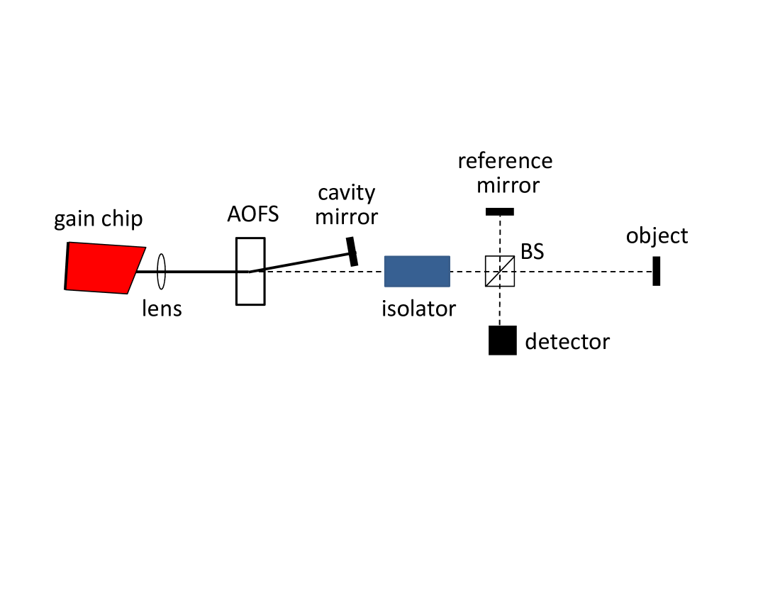
Figure 11: Schematics of the linear-cavity FSF-laser setup, with a gain chip, a collimating lens, an acousto-optic frequency shifter (AOFS) and an interferometer with 50:50 beam splitter (BS), a reference mirror, the object and the detector. An optical isolator prevents feedback into the laser. For recording the data shown in Fig. 13 and 14, the cavity mirror was replaced by a diffraction grating and the zero-order reflection of that grating used as output beam.

The cavity is closed via the frequency-shifted first diffraction order of the AOFS. Thus, the net frequency-shift per round trip is $\Delta=2\Delta_{AOFS}=160$ MHz, leading to a ”chirp rate” of $\gamma_{c}=2.1\cdot 10^{17}$ Hz/s. Typically, the undiffracted beam of the latter with a power of a few mW is used for the measurements. A 50:50 beam-splitter cube (BS) sends this beam to both, the reference surface and the object, some 8 cm away. The light, returning from these two surfaces, is recombined at the same BS and sent to the detector. The frequency of the oscillating component of the detector output is measured by frequency counting (Tektronix FCA3003).

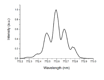
Figure 12: Optical spectrum of the linear-cavity semiconductor FSF-laser radiation.

Figure 12 shows a spectrum of the linear-cavity semiconductor FSF-laser radiation with its central wavelength near $\lambda_{c}=772.6$ nm and an overall width of 0.4 nm. The residual reflection on the output facet of the gain chip leads to the mode structure seen in Fig. 12, with the separation $\Delta_{chip}$ of the peaks given by the dimension of the gain chip. The individual spectral components of width $\leq 0.08$ nm are mutually incoherent. Therefore, the bandwidth which determines the accuracy in a ranging experiment is relatively small.

Experiments are typically done with an output power of $P=10$ mW. Because of the low output power and small effective bandwidth of the optical spectrum, the data shown below serve as proof of principle rather than as convincing documentation of the full potential of this approach. For practical ranging application power amplification is needed, e.g. by a tapered amplifier. Amplification does not modify the essential spectral properties of the radiation emitted by the FSF laser. Furthermore, suitable modification of the gain chips is likely to lead to a larger coherence bandwidth and thus to a higher accuracy of ranging results.

5.4 Results

The beat frequency, $\Omega_{beat}$, is measured over a range of about 30 mm as shown in Fig. 13(a). The variation of the accuracy of the measurement for the fixed distance of $\Delta z=83$ mm with the gate time during which the frequency is measured by counting oscillation periods is shown in Fig. 13(b) and Fig. 14. Each entry is based on 10³ individual runs. Fig. 13(b) shows the mean frequency and $1\sigma$-width of the distribution of recorded frequencies, while Fig. 14 shows the data of 13(b) converted to the $1\sigma$-width of the related distribution of readings for the distance.

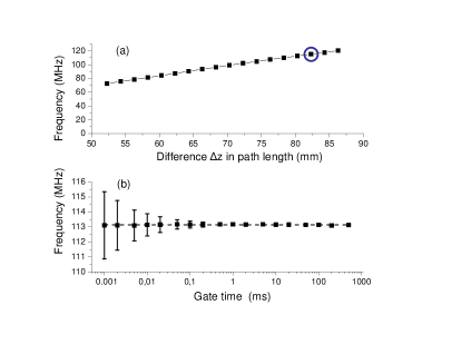
Figure 13: (a) The variation of the center frequency of the beat signals as a function of the distance $\Delta z$. This variation is consistent with the ”chirp rate” $\gamma_{c}=2.1\cdot 10^{17}$ Hz/s, given by the AOFS frequency and the cavity roundtrip time. (b) The variation of the $1\sigma$-value of the distribution of results from 10³ frequency measurements (taken at the distance marked by the circle in frame (a)) with gate time during which oscillation periods are counted. It is a most important feature that the mean of the measurement does not change when the gate time is varied over nearly six orders of magnitude.

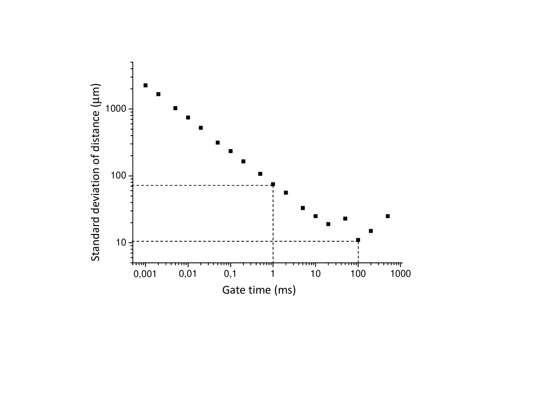
Figure 14: Variation of the standard deviation $\sigma$ of distance measurement. We find $\sigma=2$ mm for a gate time of 1 $\mu$s and $\sigma=80$ $\mu$m for a gate time of 1 ms. For a gate time $>10$ ms the limit of $\sigma\geq 10$ $\mu$m is approached.

An important observation from Fig. 13(b) is the fact that the mean value of the frequency measurement (for fixed distance), does not change when the gate time is varied over nearly six orders of magnitude. The data shown in Fig. 14 confirm the typical trade-off between accuracy and data collection time. When the gate time is 1 $\mu$s (allowing a measurement rate of the order of 1 MHz) the uncertainty of a measurement is 2 mm. That uncertainty shrinks to about 75 $\mu$m when the gate time is 1 ms (allowing a measurement rate of the order of 1 kHz). The accuracy continues to improve with further increase of the gate duration and approaches the level of $\sigma=10$ $\mu$m. The influence of systematic errors becomes relevant for gate times longer than 100 ms.

6 SUMMARY AND OUTLOOK

We have presented results based on powerful modifications of schemes for ranging using FSF-laser radiation, characterized through (i) the implementation of a novel scheme with injection of phase-modulated single-mode radiation into the cavity for accurate (order of $\mu$m) measurements or (ii) by using frequency counting for fast measurements (order of MHz rate). For (i) we used doped fibers as gain medium exploiting the large gain bandwidth of the laser transitions leading to the large bandwidth (about 5 nm) of the generated frequency comb with smooth envelope. Such a laser is robust and compact and thus suitable for operation in an industrial environment. For (ii) we used a semiconductor gain medium with the high linear gain and saturation power. Such a FSF laser can be realized with a short cavity providing short round-trip time ($\leq 1$ ns) necessary for high-speed ranging.

Equations (1) and (13) reveal a striking similarity of the FMCW-Ladar technique with the FSF-approach. Although the physics behind the signal generation is distinctly different, it is in both cases a parameter $\gamma_{c}$ which maps ”distance” onto ”frequency”. In FMCW-Ladar $\gamma_{c}$ characterizes the chirp of the radiation with a periodic, saw tooth like, change of the frequency. For precision of the measurements $\gamma_{c}$ must be constant, meaning that efforts are needed to assure that the chirp is strictly linear across the entire bandwidth which is covered. In FSF ranging $\gamma_{c}$ is typically (much) larger, meaning that a given distance $z_{obj}$ is mapped onto a (much) larger frequency. Furthermore, because in FSF ranging $\gamma_{c}$ is given by well controlled parameters (the frequency shift $\Delta$ induced by the an acousto-optic frequency shifter and the cavity round-trip time $\tau$) it is straight forward to keep it constant to very high precision. Finally, because the seeding (either by the injected radiation or by spontaneous emission within the gain medium) occurs continuously followed by frequency shift across the gain profile, the radiation is truly continuous.

An obvious next step is to go beyond the current arrangement with circular focus and a single detector and use, for even higher speed of scanning surfaces of objects, a cylindrical focus and a linear array of detectors or even a planar array of detectors when the entire surface of the object surface is illuminated by the FSF radiation.

7 ACKNOWLEDGMENT

We acknowledge support from the German ”Bundesministerium für Bildung und Forschung” (BMBF) under the projects numbered 13-N-9345 and 13-N-9346. K.B. acknowledges additional support from the research center OPTIMAS of the state of Rhineland-Palatinate. We also thank B.W.Shore for carefully reading the manuscript.

References

- (1) L.P. Yatsenko, B.W. Shore, K. Bergmann: Ranging and Interferometry with a Frequency Shifted Feedback Laser. Opt. Commun. 242, 581–598 (2004)
- (2) L.P. Yatsenko, B.W. Shore, K. Bergmann: An intuitive picture of optical ranging using frequency shifted feedback lasers seeded by a phase modulated field. Opt. Commun. 282, 2212–2216 (2009)
- (3) V.V. Ogurtsov, L.P. Yatsenko, V.M. Khodakovskyy, B.W. Shore, G. Bonnet, K. Bergmann: High Accuracy Ranging with Yb3+-doped Fiber-Ring Frequency-shifted Feedback Laser with Phase-modulated Seed. Opt. Commun. 266, 266–273 (2006)
- (4) V.V. Ogurtsov, V.M. Khodakovsky, L.P. Yatsenko, G. Bonnet, B.W. Shore, K. Bergmann: An all-fiber frequency-shifted feedback laser for optical ranging; signal variation with distance. Opt. Commun. 281, 1679–1685 (2008)
- (5) T.W. Hänsch: Nobel Lecture: Passion for precision. Rev. Mod. Phys. 78, 1297–1309 (2006)
- (6) W. Streifer, J.R. Whinnery: Analysis of a Dye Laser Using the Acousto-Optic Filter. Appl. Phys. Lett. 17, 335-337 (1970)
- (7) D.J. Taylor, S.E. Harris, S.T.K. Nieh, T.W. Hänsch: Electronic Tuning of a Dye Laser Using the Acousto-Optic Filter. Appl. Phys. Lett. 19, 269–271 (1971)
- (8) F.V. Kowalski, J.A. Squier, J.T. Pinckney: Pulse generation with an acousto-optic frequency shifter in a passive cavity. Appl. Phys. Lett. 50, 711–713 (1987)
- (9) F.V. Kowalski, S.J. Shattil, P.D. Hale: Optical pulse generation with a frequency shifted feedback laser. Appl. Phys. Lett. 53, 734–736 (1988)
- (10) G. Bonnet, S. Balle, Th. Kraft, K. Bergmann, Dynamics and Self-Modelocking of a Titanium-Sapphire Laser with Intracavity Frequency Shifted Feedback. Opt. Commun. 123, 790–800 (1996)
- (11) F.V. Kowalski, P.D. Hale, S.J. Shattil: Broadband continuous-wave laser. Opt. Lett. 13, 622–624 (1988)
- (12) P.D. Hale, F.V. Kowalski: Output characterization of a frequency shifted feedback laser: theory and experiment. IEEE J. Quant. Electron. 26, 1845–1851(1990)
- (13) I.C.M. Littler, S. Balle, K. Bergmann: Continuous-wave Laser without Frequency-domain-mode Structure: Investigation of Emission Properties and Build-up Dynamics. J. Opt. Soc. Am. B 8, 1412–1420 (1991)
- (14) I.C.M. Littler, S. Balle, and K. Bergmann: The cw Modeless Laser: Spectral Control, Performance Data and Build-up Dynamics. Opt. Commun. 88, 514–522 (1992)
- (15) S. Balle, F.V. Kowalski, K. Bergmann: Frequency Shifted Feedback Dye Laser Operating at a Small Shift Frequency. Opt. Commun. 102, 166–174 (1993)
- (16) F.V. Kowalski, S. Balle,I.C.M. Littler, K.Bergmann: Lasers with internal frequency-shifted feedback. Opt. Eng. 33, 1146–1151(1994)
- (17) K. Nakamura, F. Abe, K. Kasahara, T. Hara, M. Sato, H. Ito: Spectral characteristics of an all solid-state frequency-shifted feedback laser. IEEE J. Quant. Electron. 33, 103–111(1997)
- (18) K. Nakamura, T.Miyahara, H. Ito: Observation of a highly phase-correlated chirped frequency comb output from a frequency-shifted feedback laser. Appl.Phys. Lett. 72, 2631–2633(1998)
- (19) P.I. Richter, L. Jakab, T.W. Hänsch, N. Adoph: A cw dye-laser tuned by an acoustooptic filter. Opt. Commun. 84, 159–161 (1991)
- (20) P.I. Richter, T. W. Hänsch: Diode lasers in external cavities with frequency-shifted feedback. Opt. Commun. 85, 414–418 (1991)
- (21) H. Sabert, E.Brinkmeyer: Pulse Generation in Fiber Lasers with Frequency Shifted Feedback. J. Lightwave Technol. 12, 1360–1368 (1994)
- (22) M. Stellpflug, G. Bonnet, B.W. Shore, K. Bergmann: Dynamics of Frequency Shifted Feedback Lasers: Simulation Studies. Opt. Express 11, 2060–2080 (2003)
- (23) J.-N. Maran, P. Besnard, S. LaRochelle: Theoretical analysis of a pulsed regime observed with a frequency-shifted-feedback fiber laser. J. Opt. Soc. Am. B 23, 1302–1311 (2006)
- (24) J. Martin, Y. Zhao, S. Balle, M.P. Fewell, K. Bergmann: Visible-wavelength diode laser with weak frequency-shifted optical feedback. Opt. Commun. 112, 109–121 (1994)
- (25) L.A. Vazquez-Zuniga, Y. Jeong: Study of a mode-locked erbium-doped frequency-shifted-feedback fiber laser incorporating a broad bandpass filter: Experimental results. Opt. Commun. 306, 1–8 (2013)
- (26) L.A. Vazquez-Zuniga, Y. Jeong: Study of a mode-locked erbium-doped frequency-shifted-feedback fiber laser incorporating a broad bandpass filter: Numerical results. Opt. Commun. 322, 54–60 (2014)
- (27) H. Chen, S.P. Chen, Z.F. Jiang, J. Hou: Diversified pulse generation from frequency shifted feedback Tm-doped fibre lasers. Sci. Rep. 6, 26431 (2016)
- (28) C. Ndiaye, T. Hara, F.V. Kowalski, H. Ito: Spectral Characteristics of a Frequency-Shifted Feedback Ring Laser Using a Semiconductor Optical Amplifier. Jpn. J. Appl. Phys. 47, 3483–3485 (2008)
- (29) M. Sellahi, M. Myara, G. Beaudoin, I. Sagnes, A. Garnache: Highly coherent modeless broadband semiconductor laser. Opt. Lett. 40, 4301–4304 (2015)
- (30) L.P. Yatsenko, B.W. Shore, K. Bergmann: Theory of a frequency shifted feedback laser. Opt. Commun. 236, 183–202 (2004)
- (31) L.P. Yatsenko, B.W.Shore, K.Bergmann: Coherence in the output spectrum of frequency shifted feedback lasers. Opt. Commun. 282, 300–309 (2009)
- (32) H.G. de Chatellusand, J.P. Pique: Coherence properties of modeless lasers. PoS, 9, 1 (2009)
- (33) H.G. de Chatellusand, J.P. Pique: Statistical properties of frequency shifted feedback lasers. Opt. Commun. 283, 71–77 (2010)
- (34) H.G. de Chatellus, E. Lacot, W. Glastre, O. Jacquin, O. Hugon: The hypothesis of the moving comb in frequency shifted feedback lasers. Opt. Commun. 284, 4965–4970 (2011)
- (35) H.G. de Chatellus, E. Lacot, W. Glastre, O. Jacquin, O. Hugon: Theory of Talbot lasers. Phys. Rev. A88, 033828 (2013)
- (36) J.P. Pique: Pulsed frequency shifted feedback laser for accurate long distance measurements: Beat order determination. Opt. Commun. 286, 233–238 (2013)
- (37) H.G. de Chatellus, O. Jacquin, O. Hugon, E. Lacot: Quiet broadband light. Phys. Rev. A90, 033810 (2014)
- (38) H.G. de Chatellus, L.R. Cortés, J. Azaña: (2016) Optical real-time Fourier transformation with kilohertz resolutions. Optica 3, 1–8 (2016)
- (39) I.C M. Littler, H.-M. Keller, U. Gaubatz, K. Bergmann: Velocity control and cooling of an atomic-beam using a modeless laser. Z. Phys. D18, 307–308 (1991)
- (40) J. Hoffnagle: Proposal for continuous white-light cooling of an atomic beam. Opt. Lett. 13, 102–104 (1988)
- (41) D.T. Mugglin, A.D. Streater, S. Balle, K. Bergmann: Observation of white light-induced drift separation of Rb isotopes. Opt. Commun. 104, 165–174 (1993)
- (42) J.R.M. Barr, G.Y. Young, M.W. Phillipe: Accurate optical frequency-interval measurement by use of nonresonant frequency comb generation. Opt. Lett. 18, 1010–1012 (1993)
- (43) M.J. Lim, C.I. Sukenik, T.H. Stiefvater, P.H. Bucksbaum, R.S. Conti: Improved design of a frequency-shifted feedback diode laser for optical pumping at high magentic field Optics. Commun. 147, 99–102 (1998)
- (44) M. Cashen, V. Bretin, H. Metcalf: Optical pumping in 4He∗ with frequency-shifted feedback amplification of light. JOSA B17, 530–533 (2000)
- (45) J.-P. Pique, S. Farinotti: Efficient modeless laser for a mesospheric sodium laser guide star. JOSA B20, 2093–2101(2003)
- (46) F. Marc, I.C. Moldovan, H. Guillet de Chatellus, J.-P. Pique: High power modeless lasers for sodium laser guide stars. Ann. Phys.-Paris 32, 83–85 (2007)
- (47) J.-P. Pique, V. Fesquet, S. Jacob: Pulsed frequency-shifted feedback laser for laser guide stars: intracavity preamplifier. Appl. Opt. 50, 6294–6301 (2011)
- (48) V.I. Romanenko, A.V. Romanenko, L.P. Yatsenko, G.A. Kazakov, A.N. Litvinov, B.G. Matisov, Y.V. Rozhdestvensky: Dark resonances in the field of frequency-shifted feedback laser radiation. J. Phys. B43, 215402 (2010)
- (49) S.Balle, K. Bergmann: Self-pulsing and instabilities in a unidirectional ring dye laser with intracavity frequency shift. Opt. Commun. 116, 136–142 (1995)
- (50) H.G. de Chatellus, O. Jacquin, O. Hugon, W. Glastre, E. Lacot, J. Marklof: Generation of ultrahigh and tunable repetition rates in CW injection-seeded frequency-shifted feedback lasers. Opt. Express 21, 15065–15074 (2013)
- (51) M.P. Nikodem, E. Kluzniak, K. Abramski: Wavelength tunability and pulse duration control in frequency shifted feedback Er-doped fiber laser. Opt. Express 17, 3299–3304 (2009)
- (52) M.P. Nikodem, K. Abramski: Controlling the frequency of the frequency-shifted feedback fiber laser using injection-seeding technique. Opt. Commun. 283, 2202–2205 (2010)
- (53) A. Lyakh, R. Barron-Jimenez, I. Dunayevskiy, R. Go, E. Tsvid, C.K.N. Patel: Progress in rapidly-tunable external cavity quantum cascade lasers with a frequency-shifted feedback. Photonics 3, 19 (2016)
- (54) H. Zhang, M. Brunel, M. Romanelli, M. Vallet: Green pulsed lidar-radar emitter based on a multipass frequency-shifting external cavity. Appl. Opt. 55, 2467–2473 (2016)
- (55) M.-C. Amann, T. Bosch, M. Lescure, R. Myllyla, M. Rioux: Laser ranging: a critical review of usual techniques for distance measurement. Opt. Eng. 40, 10–19 (2001)
- (56) P. de Groot: Unusual techniques for absolute distance measurement. Opt. Eng. 40, 28–32 (2001)
- (57) J. Geng: Structered-light 3D surface imaging. Adv. Opt. Photon. 3, 128–160 (2011)
- (58) G. Berkovic, E.Shafir: Optical methods for distance and displacement measurements. Adv. Opt. Photon. 4, 441–471 (2012)
- (59) P.J. Delfyett, D. Mandridis, M.U. Piracha, D. Nguyen, K. Kim, S. Lee: Chirped pulse laser sources and applications. Prog. Quant. Electron. 36, 475–540 (2012)
- (60) I.Coddington, W.C. Swann, L. Nenadovic, N.R. Newbury: Rapid and precise absolute distance measurements at long range. Nature Photon. 3, 352–356 (2009)
- (61) J. Lee, Y.-J. Kim, K. Lee., S. Lee, S.-W. Kim: Time-of-flight measurement with femtosecond light pulses. Nature Photon. 4, 716–720 (2010)
- (62) S.A. van den Berg, S.T. Persijn, G.I.P. Kok, M.G. Zeiouny, a N.Bhattacharya: Many-wavelength interferometry with thousands of lasers for absolute distancemeasurement. Phys. Rev. Lett. 108, 183901 (2012)
- (63) E. Baumann, F.R. Giorgetta, J.D. Deschênes, W.C. Swann, I. Coddington, N.R. Newbury: Comb-calibrated laser ranging for three-dimensional surface profiling with micrometer-level precision at a distance. Opt. Express 22, 24914–24928 (2014)
- (64) Y. Liang, J. Huang, M. Ren, B. Feng, X. Chen, E Wu, G. Wu, H. Zeng: 1550-nm time-of-flight ranging system employing laser with multiple repetition rates for reducing the range ambiguity. Opt. Express 22, 4662–4670 (2014)
- (65) R. Yang, F. Pollinger, K. Meiners-Hagen, M. Krystek, J. Tan, H. Bosse: Absolute distance measurement by dual-comb interferometry with multi-channel digital lock-in phase detection. Meas. Sci. Technol. 26, 084001 (2015)
- (66) S.A. van den Berg, S. van Eldik, N. Bhattacharya: Mode-resolved frequency comb interferometry for high-accuracy long distance measurement. Sci. Rep. 5, article number: 14661 (2015)
- (67) Y.-S. Jang, G. Wang, H.J. Kang, B.J. Chun, Y.-J. Kim, S.-W. Kim: Comb-referenced laser distance interferometer for industrial nanotechnology. Sci. Rep. 6, article number: 31770 (2016)
- (68) D.J. Webb, R.M. Taylor, J.D.C. Jones, D.A. Jackson: Interferometric optical path difference measurement using sinusoidal frequency modulation of a diode laser. Opt. Commun. 66, 245–247(1988)
- (69) K. Nakamura, T. Hara, M. Yoshida, T. Miyahara, H.Ito: Optical frequency domain ranging by a frequency-shifted feedback laser. IEEE J.Quant.Electron. 36, 305–316 (2000)
- (70) H. Ito, T. Hara, C. Ndiaye: Frequency-shifted-feedback laser for precise remote 3D measurement for industry applications. Rev. Laser Eng. Suppl. 2008 36, 1038–1041 (2008)
- (71) C. Ndiaye, T. Hara, H. Ito: Performance of a solid-state frequency-shifted feedback laser in optical ranging. JEOS: RP 4, 09010 (2009)
- (72) S. Umemoto, M. Fujii, N. Miyamoto, T. Okamoto, T. Hara, H. Ito, Y. Fujino: Deflection measurement for bridges with frequency-shifted feedback laser. Proceedings of the Bridge Maintenance, Safety, Management and Life-cycle Optimization, 2570–2574 (2010)
- (73) V.V. Ogurtsov, L.P. Yatensko, V.M. Khodakovskyy, B.W. Shore, G. Bonnet, K. Bergmann: Experimental characterization of an Yb3+-doped fiber ring laser with frequency-shifted feedback. Opt. Commun. 266, 627–637 (2006)
- (74) K.A. Shore, D.M.Kane: Optimum modulation frequency for FM seeded FSF laser ranging. IEEE Proc-Optoelectronics 153, 284–286(2006)
- (75) M. F. Brandl, O. D. Mücke: Narrow-linewidth chirped frequency comb from a frequency-shifted feedback Ti:sapphire laser seeded by a phase-modulated single-frequency fiber laser. Opt. Lett. 4223–4225 (2010)
- (76) J. Paul, Y. Hong, P.S. Spencer, I. Pierce, K.A. Shore: Simple and accurate optical frequency domain ranging using off-the-shelf dfb lasers subject to frequency-shifted optical feedback. IEEE Photon. Technol. Lett. 19, 1708–1710 (2007)
- (77) J. Paul, Y. Hong, P.S. Spencer, I. Pierce, K. A.Shore: Optical frequency-domain ranging using a frequency-shifted feedback distributed-feedback laser. IET Optoelectron, 1, 277–279 (2007)
- (78) A. Dieckmann and M.Amann: Frequency modulated continous-wave lidar. SPIE Proc. 2271, 134 (1994)
- (79) A.B. Mateo, Z.W. Barber: Precision and accuracy testing of FMCW ladar-based length metrology. Appl. Opt. 54, 6019–6024 (2015)
- (80) K. Bergmann, L.P. Yatsenko, G. Bonnet, B.W. Shore: Method and device for measuring distance. European patent EP1470621 (2003) and United states patent US 7684019 (2010)
- (81) K. Kasahara, K. Nakamura, M. Sato, H. Ito: Dynamic properties of an all solid-state frequency-shifted feedback laser. IEEE J. Quantum Electron. 34, 190–203 (1998).
- (82) M.G. Littmann, H.J. Metcalf: Spectrally resolved narrow pulsed dye laser without beam expander. Appl. Opt. 17, 2224–2227 (1978)
- (83) K. Liu, M.G. Littman: Novel geometry for single-mode scanning of tunable lasers. Opt. Lett. 6, 117–18 (1981)
- (84) B. Edlen: The Refractive Index of Air Metrologia, 2, 71-80 (1966).
- (85) F. Aflatouni, B. Abiri, A. Rekhi, A. Hajimiri: Nanophotonic coherent imager. Opt. Express 23, 5117–5125 (2015)
- (86) J.V. Moloney, J. Hader, S.W. Koch: Quantum design of semiconductor active materials. Laser&Photon. Rev. 1, 24–43 (2007)