A PTAS for Three-Edge Connectivity in Planar Graphs

Abstract

We consider the problem of finding the minimum-weight subgraph that satisfies given connectivity requirements. Specifically, given a requirement $r\in\{0,1,2,3\}$ for every vertex, we seek the minimum-weight subgraph that contains, for every pair of vertices $u$ and $v$, at least $\min\{r(v),r(u)\}$ edge-disjoint $u$-to-$v$ paths. We give a polynomial-time approximation scheme (PTAS) for this problem when the input graph is planar and the subgraph may use multiple copies of any given edge. This generalizes an earlier result for $r\in\{0,1,2\}$. In order to achieve this PTAS, we prove some properties of triconnected planar graphs that may be of independent interest.

This material is based upon work supported by the National Science Foundation under Grant No. CCF-1252833.

1 Introduction

The survivable network design problem aims to find a low-weight subgraph that connects a subset of vertices and will remain connected despite edge failures, an important requirement in the field of telecommunications network design. This problem can be formalized as the $I$-edge connectivity problem for an integer set $I$ as follows: for an edge-weighted graph $G$ with a requirement function on its vertices $r:V(G)\to I$, we say a subgraph $H$ is a feasible solution if for any pair of vertices $u,v\in V(G)$, $H$ contains $\min\{r(u),r(v)\}$ edge-disjoint $u$-to-$v$ paths; the goal is to find the cheapest such subgraph. In the relaxed version of the problem, $H$ may contain multiple (up to $\max I$) copies of $G$’s edges ($H$ is a multi-subgraph) in order to achieve the desired connectivity, paying for the copies according to their multiplicity; otherwise we refer to the problem as the strict version. Thus $I=\{1\}$ corresponds to the minimum spanning tree problem and $I=\{0,1\}$ corresponds to the minimum Steiner tree problem. Here our focus is when $\max I\geq 2$.

This problem and variants have a long history. The $I$-edge connectivity problem, except when $I=\{1\}$, is MAX-SNP-hard [12]. There are constant-factor approximation algorithms for the strict $\{2\}$-edge-connectivity problem, with the best factor being 5/4 due to Jothi, Raghavachari and Varadarajan [15, 19, 18]. Ravi [24] gave a 3-approximation for the strict $\{0,2\}$-edge-connectivity problem and Klein and Ravi [23] gave a 2-approximation for the strict $\{0,1,2\}$-edge-connectivity problem. For general requirement, Jain [17] gave a 2-approximation for both the strict version and the relaxed version of the problem.

We study this problem in planar graphs. In planar graphs, the $I$-edge connectivity problem, except when $I=\{1\}$, is NP-hard (by a reduction from Hamiltonian cycle). Berger, Czumaj, Grigni, and Zhao [4] gave a polynomial-time approximation scheme (PTAS) for the relaxed $\{1,2\}$-edge-connectivity problem, and Berger and Grigni [5] gave a PTAS for the strict $\{2\}$-edge-connectivity problem. Borradaile and Klein [8] gave an efficient PTAS (EPTAS) for the relaxed $\{0,1,2\}$-edge-connectivity problem. The only planar-specific algorithm for non-spanning, strict edge-connectivity is a PTAS for the following problem: given a subset $R$ of edges, find a minimum weight subset $S$ of edges, such that for every edge in $R$, its endpoints are two-edge-connected in $R\cup S$ [22]; otherwise, the best known results for the strict versions of the edge-connectivity problem when $I$ contains 0 and 2 are the constant-factor approximations known for general graphs.

In this paper, we give an EPTAS for the relaxed $\{0,1,2,3\}$-edge-connectivity problem in planar graphs. This is the first PTAS for connectivity beyond 2-connectivity in planar graphs:

Theorem 1.

For any $\epsilon>0$ and any planar graph instance of the relaxed $\{0,1,2,3\}$-edge connectivity problem, there is an $O(n\log n)$-time algorithm that finds a solution whose weight is at most $1+\epsilon$ times the weight of an optimal solution.

In order to give this EPTAS, we must prove some properties of triconnected (three-vertex connected) planar graphs that may be of independent interest. One simple-to-state corollary of the sequel is:

Theorem 2.

In a planar graph that minimally pairwise triconnects a set of terminal vertices, every cycle contains at least two terminals.

In the remainder of this introduction we overview the PTAS for network design problems in planar graphs [8] that we use for the relaxed $\{0,1,2,3\}$-edge connectivity problem. In this overview we highlight the technical challenges that arise from handling 3-edge connectivity. We then overview why we use properties of vertex connectivity to address an edge connectivity problem and state our specific observations about triconnected planar graphs that we require for the PTAS framework to apply. In the remainder, 2-ECP refers to “the relaxed $\{0,1,2\}$-edge-connectivity problem” and 3-ECP refers to “the relaxed $\{0,1,2,3\}$-edge-connectivity problem”.

1.1 Overview of PTAS for 2-ECP

The planar PTAS framework grew out of a PTAS for travelling salesperson problem [21] and has been used to give PTASes for Steiner tree [7, 10], Steiner forest [3] and 2-EC [8] problems. For simplicity of presentation, we follow the PTAS whose running time is doubly exponential in $1/\epsilon$ [7]; this can be improved to singly exponential as for Steiner tree [10]. Note that for all these problems (except Steiner forest, which requires a preprocessing step to the framework), the optimal value of the solution is within a constant factor of the optimal value of a Steiner tree on the same terminal set where we refer to vertices with non-zero requirement as terminals. Let OPT be the weight of an optimal solution to the given problem.

The PTAS for 2-ECP relies on an algorithm to find the mortar graph $MG$ of the input graph $G$. The mortar graph is a grid-like subgraph of $G$ that spans all the terminals and has total weight bounded by $f(\epsilon)$ times the minimum weight of a Steiner tree spanning all the terminals. To construct the mortar graph, we can first find an approximate Steiner tree for all terminals and then recursively augment it with some short paths. For each face of the mortar graph, the subgraph of $G$ that is enclosed by that face (including the boundary of the face) is called a brick. It is shown that there is a nearly optimal solution for 2-ECP whose intersection with each brick is a set of non-crossing trees [8]. Further, it is proved that each such tree has only $g(\epsilon)$ leaves and its leaves are a subset of a designated vertex set, called portals, on the boundary, allowing these trees to be computed efficiently [13].

In the following, $O$-notation hides factors depending on $\epsilon$ that only affect the running time. The PTAS for 2-ECP consists of the following steps:

Step 1:

Find a subgraph that satisfies two properties: its weight is at most $O(\mathrm{OPT})$ and it contains a $(1+\epsilon)$-approximate solution. Such a subgraph is often referred to as a spanner in the literature. It is sufficient to solve the problem in the spanner.

(1)

Find the mortar graph $MG$.

(2)

For each brick of $MG$, designate as portals a constant number (depending on $\epsilon$) of vertices on the boundary of each brick.

(3)

Find Steiner trees for each subset of portals in each brick by the algorithm of Erickson et al. [13]. All the Steiner trees of each brick together with mortar graph $MG$ form the spanner.

Step 2:

Decompose the spanner into a set of subgraphs, called slices, that satisfy the following properties.

(1)

Each slice has bounded branchwidth.

(2)

Any two slices share at most one simple cycle.

(3)

Each edge can belong to at most two slices; such edges form the boundaries of slices.

(4)

The weight of all edges that belong to two slices is at most $\epsilon\mathrm{OPT}$.

Step 3:

Select a set of “artificial” terminals with connectivity requirements on the boundaries of slices from the previous step to achieve the following:

• For each slice, there is a feasible solution with respect to original and artificial terminals whose weight is bounded by the weight of the slice’s boundary plus the weight of the intersection of an optimal solution with the slice.

• The union over all slices of such feasible solutions is a feasible solution for the original graph.

Step 4:

Solve the 2-ECP with respect to original and artificial terminals in each slice by dynamic programming.

Step 5:

Convert the optimal solutions from the previous step to a solution for the spanner.

We can construct the spanner in $O(n\log n)$ time [10]. We can identify the boundary edges in Step 2 by doing breadth-first search in the planar dual and then applying the shifting technique of Baker [2], which can be done in linear time. With these edges we can decompose the spanner into slices in linear time. Step 3 can be done in linear time since the slices form a tree structure and we only need to choose as a new terminal any vertex on the boundary cycle if the cycle separates any two original terminals. If a boundary cycle separates two terminals requiring two-edge connectivity, the connectivity requirement of the new terminal on that cycle is 2, otherwise 1. By standard dynamic programming techniques we can solve the 2-ECP in the graph with bounded branchwidth in linear time. Step 5 can be done in linear time. So the total running time of the PTAS for 2-ECP is $O(n\log n)$.

We will generalize this PTAS to 3-ECP. The differences for 3-ECP are Step 3 and Step 4. For Step 3, we set the connectivity requirement of the new terminal to 3 if its corresponding boundary cycle separates two terminals requiring three-edge connectivity. For Step 4, we use the dynamic programming for $k$-ECP on graphs with bounded branchwidthgiven in Section 5, , which is inspired by that for the $k$-vertex-connectivity spanning subgraph problem in Euclidean space given by Czumaj and Lingas in [11, 12].

To prove this PTAS is correct, we need to show the subgraph obtained from Step 1 is a spanner for 3-ECP, which is the challenge of this work (as with most applications of the PTAS framework). For any fixed $0<\epsilon<1$ and input graph $G$, a subgraph $H$ of $G$ is a spanner for 3-ECP, if it has the following two properties.

(1)

The weight of $H$ is at most $O(\mathrm{OPT})$.

(2)

There is a $(1+\epsilon)$-approximate solution using only the edges of $H$.

The weight of the spanner found in Step 1 is at most $f(\epsilon)$ times the minimum weight of a Steiner tree spanning all the terminals. Since $\mathrm{OPT}$ is more than the minimum weight of a Steiner tree, the weight of our spanner is at most $O(\mathrm{OPT})$. The second property will be guaranteed by the following Structure Theorem, which is the main focus of this paper.

Theorem 3 (Structure Theorem).

For any $\epsilon>0$ and any planar graph instance $(G,w,r)$ of 3-ECP, there exists a feasible solution $S$ in our spanner such that

• the weight of $S$ is at most $(1+c\epsilon)\mathrm{OPT}$ where $c$ is an absolute constant, and

• the intersection of $S$ with the interior of any brick is a set of trees whose leaves are on the boundary of the brick and each tree has a number of leaves depending only on $\epsilon$.

The interior of a brick is all the edges of a brick that are not on the boundary. We denote the interior of a brick $B$ by $\mathrm{int}(B)$. Consider a brick $B$ of $G$ whose boundary is a face of $\mathrm{MG}$ and consider the intersection of $\mathrm{OPT}$ with the interior of this brick, $\mathrm{OPT}\cap\mathrm{int}(B)$. To prove the Structure Theorem, we will show that:

P1:

$\mathrm{OPT}\cap\mathrm{int}(B)$ can be partitioned into a set of trees $\mathcal{T}$ whose leaves are on the boundary of $B$.

P2:

If we replace any tree in $\mathcal{T}$ with another tree spanning the same leaves, the result is a feasible solution.

P3:

There is another set of $O(1)$ trees $\mathcal{T}^{\prime}$ that costs at most a $1+\epsilon$ factor more than $\mathcal{T}$, such that each tree of $\mathcal{T}^{\prime}$ has $O(1)$ leaves and $(\mathrm{OPT}\setminus{\mathcal{T}})\cup{\mathcal{T}}^{\prime}$ is a feasible solution.

Property P1 implies that we can decompose an optimal solution into a set of trees inside of bricks. Property P2 shows that we can treat those trees independently with regard to connectivity, and this gives us hope that we can replace $\mathrm{OPT}\cap\mathrm{int}(B)$ with some Steiner trees with terminals on the boundary which we can efficiently compute in planar graphs [13]. Property P3 shows that we can compute an approximation to $\mathrm{OPT}\cap\mathrm{int}(B)$ by guessing $O(1)$ leaves. Those approximations can be combined efficiently in the remaining steps of the PTAS.

For the Steiner tree problem, P1 and P2 are nearly trivial to argue; the bulk of the work is in showing P3 [7].

For 2-ECP, P1 depends on first converting $G$ and $\mathrm{OPT}$ into $G^{\prime}$ and $\mathrm{OPT}^{\prime}$ such that $\mathrm{OPT}^{\prime}$ biconnects (two-vertex connects) the terminals requiring two-edge connectivity and using the relatively easy-to-argue fact that every cycle of $\mathrm{OPT}^{\prime}$ contains at least one terminal. By this fact, a cycle in $\mathrm{OPT}^{\prime}$ must contain a vertex of the brick’s boundary (since $MG$ spans the terminals), allowing the partition of $\mathrm{OPT}^{\prime}\cap\mathrm{int}(B)$ into trees. P2 and P3 then require that two-connectivity across the brick is maintained.

For 3-ECP, P1 is quite involved to show, but further to that, showing Property P2 is also involved; the issues are illustrated in Figure 1 and are the focus of Sections 2 and 3. As with 2-ECP, we convert $\mathrm{OPT}$ into a vertex connected graph to simplify the arguments. Given Properties P1 and P2, we illustrate Property P3 by following a similar argument as for 2-ECP; since this requires reviewing more details of the PTAS framework, we cover this in Section 4.

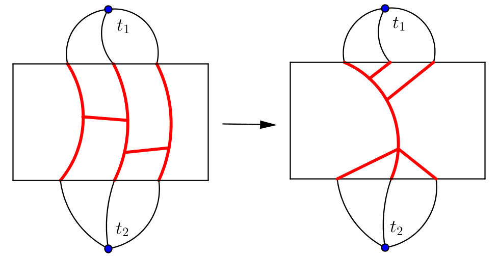
Figure 1: If the bold red tree (left) is $\mathrm{OPT}\cap\mathrm{int}(B)$ (where $B$ is denoted by the rectangle), replacing the tree with another tree spanning the same leaves (right) could destroy 3-connectivity between $t_{1}$ and $t_{2}$. We will show that such a tree cannot exist in a minimally connected graph.

Non-planar graphs

We point out that, while previously-studied problems that admit PTASes in planar graphs (e.g. independent set and vertex cover [2], TSP [21, 20, 1], Steiner tree [10] and forest [3], 2-ECP [8]) generalize to surfaces of bounded genus [6], the method presented in this paper 3-ECP cannot be generalized to higher genus surfaces. In the generalization to bounded genus surfaces, the graph is preprocessed (by removing some provably unnecessary edges) so that one can compute a mortar graph whose faces bound disks. This guarantees that even though the input graph is not planar, the bricks are; this is sufficient for proving above-numbered properties in the case of TSP, Steiner tree and forest and 2-ECP. However, for 3-ECP, in order to prove P2, we require global planarity, not just planarity of the brick. To the authors’ knowledge, this is the only problem that we know to admit a PTAS in planar graphs that does not naturally generalize to toroidal graphs.

1.2 Reduction to vertex connectivity

Here we give an overview of how we use vertex connectivity to argue about the structural properties of edge-connectivity required for the spanner properties. First some definitions. Vertices $x$ and $y$ are $k$-vertex-connected in a graph $G$ if $G$ contains $k$ pairwise vertex disjoint $x$-to-$y$ paths. If $k=3$ ($k=2$), then $x$ and $y$ are also called triconnected (biconnected). For a subset $Q$ of vertices in $G$ and a requirement function $r:Q\to\{2,3\}$, subgraph $H$ is said to be $(Q,r)$-vertex-connected if every pair of $x$ and $y$ in $Q$ is $k$-vertex-connected for $k=$min$\{r(x),r(y)\}$. We call vertices of $Q$ terminals. If $r(x)=3$ ($r(x)=2$) for all $x\in Q$, we say $H$ is $Q$-triconnected ($Q$-biconnected). We say a $(Q,r)$-vertex-connected graph is minimal, if deleting its any edge or vertex violates the connectivity requirement.

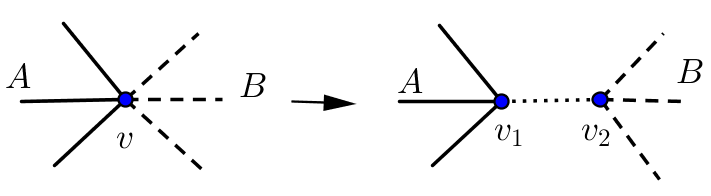
Figure 2: Vertex $v$ is cleaved into vertices $v_{1}$ and $v_{2}$. The edges incident to $v$ are partitioned into two sets $A$ and $B$ to become incident to distinct copies.

We cleave vertices to create a subgraph $\mathrm{OPT}^{\prime}$ of graph $G^{\prime}$ that is a vertex-connected version of the $\{0,1,2,3\}$-edge-connected multisubgraph $\mathrm{OPT}$ of $G$. Informally, cleaving a vertex means splitting the vertex into two copies and adding a zero-weight edge between the copies; incident edges choose between the copies in a planarity-preserving way (Figure 2). We show in Section 4.2.2 how to cleave the vertices of $\mathrm{OPT}$ so that if two terminals are $k$-edge-connected in $\mathrm{OPT}$, there are corresponding terminals in $\mathrm{OPT}^{\prime}$ that are $k$-vertex-connected. We will argue that $\mathrm{OPT}^{\prime}$ satisfies Properties P1 and P2 and these two properties also hold for OPT, since OPT^′ is obtained from OPT by cleavings.

To prove that $\mathrm{OPT}^{\prime}$ satisfies Property P1, we show that every cycle in OPT^′ contains at least one terminal (Section 2). To prove that $\mathrm{OPT}^{\prime}$ satisfies Property P2, we define the notion of a terminal-bounded component: a connected subgraph is a terminal-bounded component if it is an edge between two terminals or obtained from a maximal terminal-free subgraph $S$ (a subgraph containing no terminals), by adding edges from $S$ to its neighbors (which are all terminals by maximality of $S$). We prove that in a minimal $Q$-triconnected graph any terminal-bounded component is a tree whose leaves are terminals and the following Connectivity Separation Theorem in Section 3:

Theorem 4 (Connectivity Separation Theorem).

Given a minimal $(Q,r)$-vertex-connected planar graph, for any pair of terminals $x$ and $y$ that require triconnectivity (biconnectivity), there are three (two) vertex disjoint paths from $x$ to $y$ in $G$ such that any two of them do not contain edges of the same terminal-bounded tree.

Corollary 5.

Given a minimal $(Q,r)$-vertex-connected planar graph, for any pair of terminals $x$ and $y$ that require triconnectivity (biconnectivity), there exist three (two) vertex disjoint $x$-to-$y$ paths such that any path that connects any two of those $x$-to-$y$ paths contains a terminal.

This can be viewed as a generalization of the following by Borradaile and Klein for 2-ECP [9]:

Theorem 6.

(Theorem 2.8 [9]). Given a graph that minimally biconnects a set of terminals, for any pair of terminals $x$ and $y$ and for any two vertex disjoint $x$-to-$y$ paths, any path that connects these paths must contain a terminal.

Note that Theorem 6 holds for general graphs while Corollary 5 only holds for planar graphs. This again underscores why our PTAS does not generalize to higher-genus graphs. Further, Theorem 6 implies that for biconnectivity any pair of disjoint $x$-to-$y$ paths has the stated property, while for triconnectivity there can be a pair of $x$-to-$y$ paths that does not have the property (See Figure 3). So Corollary 5 is the best that we can hope, since it shows there exists a set of disjoint paths that has the stated property; higher connectivity comes at a price.

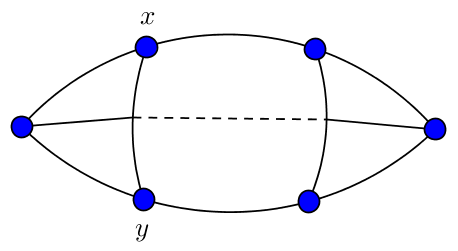
Figure 3: A minimal $Q$-triconnected graph. The bold vertices are terminals. The dashed path connects two $x$-to-$y$ paths but it does not contain any terminal.

For OPT^′, Corollary 5 implies Property P2. Consider the set of disjoint paths guaranteed by Corollary 5. If any tree replacement in a brick merges any two disjoint paths, say $P_{1}$ and $P_{2}$, in the set (the replacement in Figure 1 merges three paths), then the replaced tree must contain at least one vertex of $P_{1}$ and one vertex of $P_{2}$. This implies the replaced tree contains a $P_{1}$-to-$P_{2}$ path $P$ such that each vertex in $P$ has degree at least two in the replaced tree. Further, $P$ contains a terminal by Corollary 5. However, all the terminals are in mortar graph, which forms the boundaries of the bricks. So $P$ must have a common vertex with the boundary of the brick. By Property P1, the replaced tree, which is in the intersection of $\mathrm{OPT}^{\prime}$ with the interior of the brick, can only contain leaves on the boundary of the brick. Therefore, the replaced tree can not contain such a $P_{1}$-to-$P_{2}$ path, otherwise there is a vertex in $P$ that has degree one in the tree. We give the complete proof in Section 4.

2 Vertex-connectivity basics

In this section, we consider minimal $(Q,r)$-vertex-connected graphs for a subset $Q$ of vertices and a requirement function $r:Q\to\{2,3\}$. A subgraph induced by $S\subseteq V(G)$ or $S\subseteq E(G)$ in $G$ is denoted by $G[S]$. The degree of vertex $v$ in $G$ is denoted by $d_{G}(v)$. By $P[a,b]$ or $T[a,b]$ we denote the $a$-to-$b$ subpath of path $P$ or tree $T$.

Lemma 7.

A minimal $(Q,r)$-vertex-connected graph is biconnected.

Proof.

For a contradiction, assume that a minimal $(Q,r)$-vertex-connected graph $H$ has a cut-vertex $u$ and let the subgraphs be $H_{i}$ for $0<i\leq k$ and $k\geq 2$ after removing $u$. Then for any vertex $x\in H_{i}$ and $y\in H_{j}$ ($i\neq j$), every $x$-to-$y$ path must contain $u$. If $H_{i}$ and $H_{j}$ ($i\neq j$) both have terminals, then terminals in those different subgraphs do not achieve the required vertex-connectivity. It follows that there exists one subgraph $H_{i}\cup\{u\}$ that contains all the terminals. For any two terminals $x,y\in H_{i}\cup\{u\}$, the paths witnessing their connectivity are simple and so can only visit $u$ once. Therefore, $H_{i}\cup\{u\}$ is a smaller subgraph that is $(Q,r)$-vertex-connected, contradicting the minimality. ∎

2.1 Ear decompositions

An ear decomposition of a graph is a partition of its edges into a sequences of cycles and paths (the ears of the decomposition) such that the endpoints of each ear belong to union of earlier ears in the decomposition. An ear is open if its two endpoints are distinct from each other. An ear decomposition is open if all ears but the first are open. A graph containing more than one vertex is biconnected if and only if it has an open ear decomposition [25]. Ear decompositions can be found greedily starting with any cycle as the first ear. It is easy to see that a more general ear decomposition can start with any biconnected subgraph:

Observation 1.

For any biconnected subgraph $H$ of a biconnected graph $G$, there exists an open ear decomposition $E_{1},E_{2},\dots,E_{k}$ of $G$ such that $H=\bigcup_{i\leq j}E_{i}$ for some $j\leq k$.

Let $G$ be a minimal $(Q,r)$-vertex-connected graph, and let $H$ be a minimal $Q_{3}$-triconnected subgraph of $G$ where $Q_{3}=r^{-1}(3)$. Then more strongly, we can assume that each ear of $G$ that are within the parts of $G\setminus H$ contains a terminal. ($G$ is biconnected by Lemma 7.) We do so by starting with an open ear decomposition of $H$ and then for each terminal that is not yet spanned in turn, we add an ear through it; such an ear exists because these terminals require biconnectivity and must have two disjoint paths to the partially constructed ear decomposition. Any remaining edges after the terminals have been spanned would contradict the minimality of $G$. Formally and more specifically:

Observation 2.

For $G$ and $H$, there is an open ear decomposition $E_{1},E_{2},\dots,E_{k}$ of $G$ such that for any component $\chi$ of $G\setminus H$, $\chi=\bigcup_{i=a}^{b}E_{i}$ for some $a\leq b\leq k$ and $E_{i}$ contains a terminal for $i=a,\ldots,b$.

Lemma 8.

For $G$ and $H$, there is an open ear decomposition $E_{1},E_{2},\dots,E_{k}$ of $G$ such that for any component $\chi=\bigcup_{i=a}^{b}E_{i}$ of $G\setminus H$, any path in $\chi$ (or $\chi\setminus E_{a}$) with both endpoints in $H$ (or $H\cup E_{a}$) strictly contains a vertex of $Q$.

Proof.

We prove the lemma for the path in $\chi$ with endpoints in $H$; the other case can be proved similarly. We prove this by induction on the index of the ear decomposition guaranteed by Observation 2. A path $P$ in $G\setminus H$ with both endpoints in $H$ belongs to a component $\chi$ of $G\setminus H$. Suppose that the lemma is true for every $H$-to-$H$ path in $\bigcup_{i=a}^{c}E_{i}$; we prove the lemma true for such a path in $\bigcup_{i=a}^{c+1}E_{i}$. Since $E_{c+1}$ is an open ear, any path with two endpoints in $H$ that uses an edge of $E_{c+1}$ would have to contain the entirety of $E_{c+1}$, which contains a terminal. ∎

2.2 Removable edges

Holton, Jackson, Saito and Wormald study the removability of edges in triconnected graphs [16]. For an edge $uv$ of a simple, triconnected graph $G$, removing $e$ consists of:

• Deleting $uv$ from $G$.

• If $u$ or $v$ now have degree 2, contract incident edges.

• If there are now parallel edges, replace them with a single edge.

The resulting graph is denoted by $G\ominus e$. If $G\ominus e$ is triconnected, then $e$ is said to be removable. We use the following theorems of Holton et al. [16].

Theorem 9 (Theorem 1 [16]).

Let $G$ be a triconnected graph of order at least six and $e\in E(G)$. Then $e$ is nonremovable if and only if there exists a set $S$ containing exactly two vertices such that $G\setminus\{e,S\}$ has exactly two components $A,B$ with $|A|\geq 2$ and $|B|\geq 2$.

In the above theorem, we call $(e,S)$ a separating pair. For a separating pair $(e,S)$ of $G$, we say $S$ is the separating set for $e$.

Theorem 10 (Theorem 2 [16]).

Let $G$ be a triconnected graph of order at least six, and let $(e,S)$ be a separating pair of $G$. Let $e=xy$, and let $A$ and $B$ be the two components of $G\setminus\{e,S\}$, $x\in A$, and $y\in B$. Then every edge joining $S$ and $\{x,y\}$ is removable.

Theorem 11 (Theorem 6 part (a) [16]).

Let $G$ be a triconnected graph of order at least six and $C$ be a cycle of $G$. Suppose that no edges of $C$ are removable. Then there is an edge $yz$ in $C$ and a vertex $x$ of $G$ such that $xy$ and $xz$ are removable edges of $G$, $d_{G}(y)=d_{G}(z)=3$ and $d_{G}(x)\geq 4$.

2.3 Properties of minimal $(Q,r)$-vertex-connected graphs

For a $Q$-triconnected graph $H$, we can obtain another graph $H^{\prime}$ by contracting all the edges incident to the vertices of degree two in $H$. We say $H^{\prime}$ is contracted version of $H$ and, alternatively, is contracted $Q$-triconnected.

Lemma 12.

A contracted minimal $Q$-triconnected graph is triconnected.

Proof.

For a contradiction, we assume that a contracted minimal $Q$-triconnected graph $H$ has a pair of cut-vertices $\{u,v\}$ and let the subgraphs be $H_{i}$ for $0<i\leq k$ and $k\geq 2$ after removing $\{u,v\}$. Then for any vertices $x\in H_{i}$ and $y\in H_{j}$ ($i\neq j$), every $x$-to-$y$ path must use either $u$ or $v$. If $H_{i}$ and $H_{j}$ ($i\neq j$) both contain terminals, then terminals in those different subgraphs do not satisfy the triconnectivity. It follows there exists one strict subgraph $H_{i}\cup\{u,v\}$ containing all the terminals. For any two terminals $x,y\in H_{i}\cup\{u,v\}$, the paths witnessing their connnectivity are simple and can only visit $u$ and $v$ once. So $H_{i}\cup\{u,v\}$ is a smaller subgraph that is $Q$-triconnected, which contradicts the minimality. ∎

Lemma 13.

If $H$ is a minimal $Q$-triconnected graph, then the contracted version of $H$ is also a minimal $Q$-triconnected graph.

Proof.

Let $H^{\prime}$ be the contracted $Q$-triconnected graph obtained from $H$. For a contradiction, assume $H^{\prime}$ is not minimal $Q$-triconnected. Then we can delete at least one edge, say $e$, in $H^{\prime}$ while maintaining $Q$-triconnectivity. Then $e$ corresponds a path in $H$, deleting which will not affect the $Q$-triconnectivity. This contradicts the minimality of $H$. ∎

Lemma 14.

For $|Q|=3$, a contracted minimal $Q$-triconnected graph is simple or a triangle with three pairs of parallel edges. For $|Q|>3$, a contracted minimal $Q$-triconnected graph is simple.

Proof.

Let $H$ be a minimal $Q$-triconnected graph, and $H^{\prime}$ the contracted graph. We have the following observation.

Observation 3.

If there are parallel edges between any pair of vertices in $H^{\prime}$, the paths witnessing the vertex-connectivity between any other pair of terminals can only use one of the parallel edges.

By the above observation, the parallel edges can only be between terminals in $H^{\prime}$.

Claim 15.

For $|Q|>2$, there can not exist three parallel edges between any two terminals in $H^{\prime}$.

Proof.

Let $t_{1}$, $t_{2}$ and $t_{3}$ be three terminals and assume there are three parallel edges, say $e_{1}$, $e_{2}$ and $e_{3}$, between $t_{1}$ and $t_{2}$. Let $P_{1}$ be the path in $H$ corresponding to $e_{1}$. We will argue that $H\setminus P_{1}$ is $Q$-triconnnected by showing that $H^{\prime}-e_{1}$ is $Q$-triconnected. There must be a path in $H^{\prime}$ from $t_{1}$ to $t_{3}$ that does not use $e_{1}$, $e_{2}$ and $e_{3}$ by Observation 3 and a path in $H^{\prime}$ from $t_{2}$ to $t_{3}$ that does not use $e_{1}$, $e_{2}$ and $e_{3}$. These paths witness a $t_{1}$ to $t_{2}$ path $R$ in $H^{\prime}$ that does not use $e_{1}$, $e_{2}$ and $e_{3}$. So after deleting $e_{1}$, $t_{1}$ and $t_{2}$ are still triconnected by $e_{2}$, $e_{3}$ and $R$. By Observation 3, deleting $e_{1}$ does not affect the triconnectivity of other pairs of terminals. ∎

We first prove the first statement of Lemma 14. Let $t_{1}$, $t_{2}$ and $t_{3}$ be the three terminals, and suppose $H^{\prime}$ is not simple; let $e_{1}$ and $e_{2}$ be parallel edges w.l.o.g. between $t_{1}$ and $t_{2}$. By Observation 3, there must be two disjoint paths in $H^{\prime}$ from $t_{1}$ to $t_{3}$ that do not use $e_{1}$ and $e_{2}$. Therefore, there is a simple cycle, called $C_{13}$, through $t_{1}$ and $t_{3}$. Similarly, there is another cycle, called $C_{23}$, through $t_{2}$ and $t_{3}$. If $C_{13}$ and $C_{23}$ have only one common vertex $t_{3}$, then $C_{13}\cup C_{23}\cup\{e_{1},e_{2}\}$ is a subgraph of $H^{\prime}$ that is $Q$-triconnected, and must be a triangle with three pairs of parallel edges by the minimality of $H^{\prime}$ and Lemma 13. If $C_{13}$ and $C_{23}$ have more than one common vertex, then $C_{13}\cup C_{23}$ contains a simple cycle through $t_{1}$ and $t_{2}$. So $H^{\prime}-e_{1}$ will be a smaller $Q$-triconnected graph, contradicting the minimality of $H^{\prime}$.

Now we prove the second statement. For any four terminals $t_{1},t_{2},t_{3},t_{4}\in Q$, without loss of generality, assume there are two parallel edges $e_{1}$ and $e_{2}$ between $t_{1}$ and $t_{2}$ in $H^{\prime}$ by Claim 15. We will prove that $H^{\prime}-e_{1}$ is also $Q$-triconnected, contradicting the minimality of $H$. To prove this, we argue that $t_{1}$ and $t_{2}$ are four-vertex-connected in $H^{\prime}$ and biconnected in $H^{\prime}\setminus\{e_{1},e_{2}\}$.

For a contradiction, we assume $t_{1}$ and $t_{2}$ are simply connected but not biconnected in $H^{\prime}\setminus\{e_{1},e_{2}\}$. By Claim 15, every other pair of terminals is at least biconnected in $H^{\prime}\setminus\{e_{1},e_{2}\}$. Consider the block-cut tree of $H^{\prime}-e_{1}$, the tree whose vertices represent maximal biconnected components and whose edges represent shared vertices between those components [14].

The biconnectivity of $t_{1}$ and $t_{3}$ implies $t_{1}$ and $t_{3}$ are in a common block $B_{13}$ in the block-cut tree. Likewise, $t_{2}$ and $t_{3}$ are in a common block $B_{23}$. If $t_{2}\in B_{13}$ then $t_{1}$ and $t_{2}$ are biconnected, a contradiction. Now we have $B_{13}\cap B_{23}=\{t_{3}\}$. The biconnectivity of $t_{1}$ and $t_{4}$ implies that $t_{1}$ and $t_{4}$ are in the same block. Since $t_{3}$ is a cut for $t_{1}$ and $t_{2}$, $t_{3}$ is also a cut for $t_{4}$ and $t_{2}$, which contradicts the biconnectivity of $t_{2}$ and $t_{4}$. So $t_{1}$ and $t_{2}$ are biconnected in $H^{\prime}\setminus\{e_{1},e_{2}\}$. ∎

Lemma 16.

Let $H$ be a contracted minimal $Q$-triconnected simple graph. Then for any $e\in E(H)$, if neither of the two endpoints of $e$ are terminals, $e$ is nonremovable.

Proof.

By Lemma 12, $H$ is triconnected. Let $e\in H$ be an edge, neither of whose endpoints are terminals. For a contradiction, suppose $e$ is removable, then $H\ominus e$ is triconnected. Since neither of the two endpoints of $e$ are terminals, $Q\subseteq V(H\ominus e)$. So $H\ominus e$ is a smaller $Q$-triconnected graph than $H$, contradicting minimality of $H$. ∎

2.4 Cycles must contain terminals

Borradaile and Klein proved that in a minimal $Q$-biconnected graph, every cycle contains a terminal (Theorem 2.5 [9]). We prove similar properties here.

Lemma 17.

Let $H$ be a contracted minimal $Q$-triconnected graph. Then every cycle in $H$ contains a vertex of $Q$.

Proof.

$H$ is triconnected by Lemma 12. If $H$ is not simple, then either $|Q|=2$ or $|Q|=3$. If $|Q|=2$, then by the minimality of $H$, $H$ consists of three parallel edges. If $|Q|=3$, then by Lemma 14, $H$ is a triangle with three pairs of parallel edges.

Now we assume $H$ is a simple graph and by Lemma 14, $|Q|\geq 3$. For a contradiction, assume there is a cycle $C$ in $H$ on which there is no terminal. Since $H$ is simple, by Lemma 16, every edge on $C$ will be nonremovable. Since $|C|\geq 3$ and $|Q|\geq 3$, $|V(H)|\geq 6$. By Theorem 11 if there is no removable edges on $C$, then there exists an edge $yz$ on $C$ and another vertex $x$ of $H$ such that $xy$ and $xz$ are removable, $d_{H}(y)=d_{H}(z)=3$ and $d_{H}(x)\geq 4$. In $H-xy$, $y$ is the only possible degree 2 vertex, and contracting $yz$ does not introduce any parallel edges, so $H\ominus xy$ contains $Q$ and is $Q$-triconnected, which contradicts the minimality of $H$. ∎

Theorem 18.

For a requirement function $r:Q\to\{2,3\}$, let $G$ be a minimal $(Q,r)$-vertex-connected graph. Then every cycle in $G$ contains a vertex of $Q$.

Proof.

Let $G^{\prime}$ be a minimal $Q$-triconnected graph that is a supergraph of $G$. Let $G^{\prime\prime}$ be the contracted minimal $Q$-triconnected graph obtained from $G^{\prime}$. Then by Lemma 17, every cycle in $G^{\prime\prime}$ contains a vertex of $Q$; $G^{\prime}$ also has this property since $G^{\prime}$ is a subdivision of $G^{\prime\prime}$ and clearly, $G$ as a subgraph of $G^{\prime}$, also has this property. ∎

Lemma 19.

Let $H$ be a contracted minimal $Q$-triconnected graph. If a cycle in $H$ only contains one vertex $v$ of $Q$, then one edge of that cycle incident to $v$ is removable.

Proof.

For a contradiction, assume both edges in the cycle incident to $v$ are nonremovable. By Lemma 16 all the other edges in the cycle are also nonremovable, so all the edges in the cycle are nonremovable. By Theorem 11, there is an edge $yz$ in the cycle and a vertex $x$ in $H$ such that $xy$ and $xz$ are removable, $d_{H}(y)=d_{H}(z)=3$ and $d_{H}(x)\geq 4$. Then one of $y$ and $z$ can not be in $Q$. W.l.o.g. assume $y$ is not in $Q$. In $H-xy$, $y$ is the only possible degree 2 vertex, and contracting $yz$ does not introduce any parallel edges, so $H\ominus xy$ contains $Q$ and is $Q$-triconnected, which contradicts the minimality of $H$. ∎

3 Connectivity Separation

In this section we continue to focus on vertex connectivity and prove the Connectivity Separation Theorem. The Connectivity Separation Theorem for biconnectivity follows easily from Theorem 6. To see why, consider two paths $P_{1}$ and $P_{2}$ that witness the biconnectivity of two terminals $x$ and $y$. For an edge of $P_{1}$ to be in the same terminal-bounded component as an edge of $P_{2}$, there would need to be a $P_{1}$-to-$P_{2}$ path that is terminal-free. However, such a path must contain a terminal by Theorem 6. Herein we mainly focus on triconnectivity.

For a requirement function $r:Q\to\{2,3\}$, let $G$ be a minimal $(Q,r)$-vertex-connected planar graph. We say a subgraph is terminal-free if it is connected and does not contain any terminals. It follows from Theorem 18 that any terminal-free subgraph of $G$ is a tree. We partition the edges of $G$ into terminal-bounded components as follows: a terminal-bounded component is either an edge connecting two terminals or is obtained from a maximal terminal-free tree $T$ by adding the edges from $T$ to its neighbors, all of which are terminals. Theorem 20 will also show that any terminal-bounded subgraph is also a tree.

For a connected subgraph $\chi$ and an embedding with outer face containing no edge of $\chi$, let $C(\chi)$ be the simple cycle that strictly encloses the fewest faces and all edges of $\chi$, if such a cycle exists. (Note that $C(\chi)$ does not exist if there is no such choice for an outer face.) In order to prove the Connectivity Separation Theorem for bi- and triconnectivity, we start with the following theorem:

Theorem 20 (Tree Cycle Theorem).

Let $T$ be a terminal-bounded component in a minimal $Q$-triconnected planar graph $H$. Then $T$ is a tree and $C(T)$ exists with the following properties

$(a)$

The internal vertices of $T$ are strictly inside of $C(T)$.

$(b)$

All vertices strictly inside of $C(T)$ are on $T$.

$(c)$

All leaves of $T$ are in $C(T)$.

$(d)$

Any pair of distinct maximal terminal-free subpaths of $C(T)$ does not contain vertices of the same terminal-bounded tree.

Theorem 2 follows from the Tree Cycle Theorem.

Proof of Theorem 2.

For a contradiction, assume there is a cycle in $H$ that only containing one terminal, then there is a terminal-bounded component containing that cycle, which can not be a tree, contradicting Tree Cycle Theorem. ∎

We give an overview of the proof the Tree Cycle Theorem in Subsection 3.2. First, let us see how the Tree Cycle Theorem implies the Connectivity Separation Theorem.

3.1 The Tree Cycle Theorem implies the Connectivity Separation Theorem

For a requirement function $r:Q\to\{2,3\}$, let $G$ be a minimal $(Q,r)$-vertex-connected planar graph. Let $Q_{3}$ be the set of terminals requiring triconnectivity, and let $H$ be a minimal $Q_{3}$-triconnected subgraph of $G$. Let $Q_{2}=Q\setminus Q_{3}$. We will prove the theorem for different types of pairs of terminals, based on their connectivity requirement. Lemma 8 allows us to focus on $H$ when considering terminals in $H$ (note that terminals of $Q_{2}$ may be in $H$), for a simple corollary of Lemma 8 is that if two trees are terminal-bounded in $H$, then they cannot be subtrees of the same terminal-bounded tree in $G$. Note that if we consider a subset of the terminals in defining free-ness of terminals, the same properties will hold for $Q$, as adding terminals only further partitions terminal-bounded trees.

3.1.1 Connectivity Separation for $\mathbf{x,y\in Q_{3}}$

For now, we consider only $Q_{3}$ to be terminals. We say connected components share a terminal-bounded tree if they contain edges (and so internal vertices) of that tree. We prove the following lemma which can be seen as a generalization of Connectivity Separation for contracted triconnected graphs. We use this generalization to prove Connectivity Separation for terminals both of which may not be in $Q_{3}$. Connectivity Separation for terminals in $Q_{3}$ follows from this lemma by considering three vertex disjoint paths paths matching $A$ to $B$ where $A=\{x,x,x\}$ and $B=\{y,y,y\}$. Note that the lemma may swap endpoints of paths; in particular, for vertex disjoint $a$-to-$b$ and $c$-to-$d$ paths, the lemma may only guarantee $a$-to-$d$ and $c$-to-$b$ paths that do not share terminal-bounded trees.

Lemma 21.

If two multisets of vertices $A$ and $B$ (where $|A|=|B|=2$, resp. $3$) satisfy the following conditions, then there are two (resp. three) internally vertex-disjoint paths from $A$ to $B$ such that no two of them share the same terminal-bounded tree.

1. Distinct vertices in $A$ are in distinct terminal-bounded trees and distinct vertices in $B$ are in distinct terminal-bounded trees.

2. There are two (resp. three) vertex-disjoint paths from $A$ to $B$.

Proof.

We prove the lemma for three paths as the two-paths version is proved by the first case of three-paths version. Let $P_{1}$, $P_{2}$ and $P_{3}$ be the three vertex disjoint paths whose endpoints are in different terminal-bounded trees. For $i=1,2,3$, let $a_{i}$ and $b_{i}$ be the endpoints of $P_{i}$. Let $\mathcal{T}$ be the collection of terminal-bounded trees shared by two or more of $P_{1},P_{2}$ and $P_{3}$. We prove, by induction on the size of $\mathcal{T}$, that we can modify the paths to satisfy Connectivity Separation. We pick a tree $T\in\mathcal{T}$ shared by (w.l.o.g.) $P_{1}$ and modify the paths so that $T$ is not shared by the new paths; further, we show that the terminal-bounded trees shared by the new paths are a subset of $\mathcal{T}\setminus\{T\}$.

We order the vertices of $P_{i}$ from $a_{i}$ to $b_{i}$ for $i=1,2,3$. Among all the trees in $\mathcal{T}$ shared by $P_{1}$, let $T$ be the tree sharing the first vertex from $a_{1}$ to $b_{1}$ along $P_{1}$. Without loss of generality, assume that $T$ is shared by $P_{2}$. ($P_{3}$ may also share $T$.) Let $C$ be the cycle guaranteed by the Tree Cycle Theorem for $T$ in $H$. Since $x$ and $y$ are terminals, they are not strictly enclosed by $C$ (property (b)). Further, $P_{1}$ and $P_{2}$ must both contain vertices of $C$ because $P_{1}$ and $P_{2}$ both contain internal vertices of $T$ and the internal vertices of $T$ are strictly enclosed by $C$ (property (a)).

Augmenting the paths First we augment each path to simplify the construction, but may make the paths non-simple. If there is a terminal-bounded tree shared by only $P_{i}$ and $C$ (and not $P_{j}$, $j\neq i$), then there is a terminal-free path from $P_{i}$ to $C$; add two copies of this path to $P_{i}$ ($P_{i}$ travels back and forth along this path). We repeat this for every possible shared tree and $i=1,2,3$. We let $P_{1},P_{2},P_{3}$ be the resulting paths. Note that adding such paths does not introduce any new shared terminal-bounded trees between $P_{1},P_{2},P_{3}$ and $P_{1},P_{2},P_{3}$ are still vertex-disjoint.

Let $u_{i}$ and $v_{i}$ be the first and last vertex of $P_{i}$ that is in $C$. There are two cases:

Case 1: $\mathbf{P_{3}}$ is disjoint from $\mathbf{C}$. In this case there were no applicable augmentations to $P_{3}$ as described above (and $u_{3}$ and $v_{3}$ are undefined). Since $T$ is the first tree in $\mathcal{T}$ along $P_{1}$, $u_{1}$ and $u_{2}$ cannot be internal vertices of the same terminal-bounded tree. Further, by planarity and disjointness of the three paths, $\{u_{1},v_{1}\}$ and $\{u_{2},v_{2}\}$ do not interleave around $C$. Let $C_{i}$ be the $u_{i}$-to-$v_{i}$ subpath of $C$ disjoint from $\{u_{3-i},v_{3-i}\}$ for $i=1,2$: $C_{1}$ and $C_{2}$ are disjoint. By construction, $P_{1}\cup P_{2}\cup C_{1}\cup C_{2}\setminus\{P_{1}[u_{1},v_{1}],P_{2}[u_{2},v_{2}]\}$ contains two disjoint $A$-to-$B$ paths; these paths replace $P_{1}$ and $P_{2}$. By the definition of $u_{i}$ and $v_{i}$ for $i=1,2$ and the above-described path augmentation, if $C_{i}$ shares a terminal-bounded tree with another path, then that tree was already in $\mathcal{T}$. Therefore we have reduced the number of shared terminal-bounded trees (since $T$ is no longer shared) without introducing any new shared terminal-bounded trees.

Case 2: $\mathbf{P_{3}}$ and $\mathbf{C}$ have at least one common vertex. In this case, $P_{3}$ may or may not contain internal vertices of $T$. By planarity and disjointness of the paths, the sets $\{u_{1},u_{2},u_{3}\}$ and $\{v_{1},v_{2},v_{3}\}$ do not interleave around $C$. Let $C_{u}$ and $C_{v}$ be the minimal subpaths of $C$ that span $\{u_{1},u_{2},u_{3}\}$ and $\{v_{1},v_{2},v_{3}\}$, respectively. Let $C_{1}$ and $C_{2}$ be the components of $C\setminus\{C_{u},C_{v}\}$. Then $C_{1}$ and $C_{2}$ are disjoint paths that connect two vertices of $\{u_{1},u_{2},u_{3}\}$ to two vertices of $\{v_{1},v_{2},v_{3}\}$.

By planarity and disjointness of the paths, there must be a leaf of $T$ that is an internal vertex of $C_{u}$ in order for paths to reach $T$ from that leaf of $T$; the same property holds for $C_{v}$. Let $C_{3}$ be the simple path from the middle vertex of $\{u_{1},u_{2},u_{3}\}$ to the middle vertex of $\{v_{1},v_{2},v_{3}\}$ in $C_{u}\cup C_{v}\cup T$. Then the to-$C$ prefices of $P_{i}$, $C_{i}$ and the from-$C$ suffices of $P_{i}$ (for $i=1,2,3$) together form three vertex-disjoint paths between the same endpoints.

The resulting path that contains $C_{3}$ is the only of the three resulting paths that contains internal vertices of $T$ since $C_{1}$ and $C_{2}$ do not share the same terminal-bounded tree because the endpoints of $C_{3}\cap T$ are terminals (property (d) of the Tree Cycle Theorem).

By the definition of $u_{i}$ and $v_{i}$ and the above-described path augmentation, if $C_{i}$ shares a terminal-bounded tree with another path, then that tree was already in $\mathcal{T}$. Therefore we have reduced the number of shared terminal-bounded trees (since $T$ is no longer shared) without introducing any new shared terminal-bounded trees. ∎

3.1.2 Connectivity Separation for $\mathbf{x,y\in H\cap Q}$

Note that $H$ may span vertices of $Q_{2}$. Let $P_{1}$ and $P_{2}$ be vertex-disjoint $x$-to-$y$ paths. The first and last edges of $P_{1}$ and $P_{2}$ are in different terminal-bounded trees, since $x$ and $y$ are terminals. If either $P_{1}$ or $P_{2}$ is an edge, then we could obtain Connectivity Separation for $x$ and $y$. Otherwise, let $x_{1}$ and $x_{2}$ be $x$’s neighbors on $P_{1}$ and $P_{2}$ respectively; similarly define $y_{1}$ and $y_{2}$. Let $P_{1}^{\prime}$ and $P_{2}^{\prime}$ be the paths guaranteed by Lemma 21 when applied to $P_{1}[x_{1},y_{1}]$ and $P_{2}[x_{2},y_{2}]$. Then $P_{1}^{\prime}\cup P_{2}^{\prime}\cup\{xx_{1},xx_{2},yy_{1},yy_{2}\}$ contain vertex disjoint $x$-to-$y$ paths that satisfy the requirements of Connectivity Separation Theorem.

3.1.3 Connectivity Separation for $\mathbf{x\in Q_{2}\setminus H,y\in Q}$

Since $x$ and $y$ only require biconnectivity, we will prove that there exists a simple cycle $C$ containing $x$ and $y$, such that every $C$-to-$C$ path strictly contains a terminal, from which Connectivity Separation follows as argued in the beginning of Section 3. The following claim gives a sufficient condition for such cycle $C$.

Claim 22.

If every terminal-bounded tree of $H$ and every component of $G\setminus E(H)$ contain at most one strict subpath of $C$, then every $C$-to-$C$ path contains a terminal.

Proof.

Let $P$ be a $C$-to-$C$ path and let $C_{\chi}$ be the subpath of $C$ in the component $\chi$ of $G\setminus H$. Then $C_{\chi}$ has two endpoints in $H$ and it must contain a terminal by Lemma 8. Every subpath of $P$ in $\chi$ has endpoints in $H\cup C_{\chi}$. We can take $C_{\chi}$ as the first ear for $\chi$, and then every subpath of $P$ in $\chi$ contains a terminal by Lemma 8. So if $P$ contains an edge of $\chi$, we have the claim.

If $P$ does not contain an edge in $G\setminus H$, then $P\subseteq H$. Further, if $P$ does not contain any terminal, then it must be in some terminal-free tree $T$ by condition of the claim $T$ contains only one subpath $C_{T}$ of $C$. Since $P$ is a $C$-to-$C$ path, $C_{T}$ and $P$ form a cycle in $T$, which contradicts $T$ is a tree. So $P$ must contain a terminal. ∎

The following claim will allow us to use Lemma 21 on parts of the $x$-to-$y$ paths.

Claim 23.

Each connected component of $G\setminus H$ has at most one non-terminal vertex in common with any terminal-bounded tree of $H$.

Proof.

For a contradiction, suppose $a$ and $b$ are two non-terminal vertices of component $\chi$ of $G\setminus H$ that are both in some terminal-bounded tree $T$ of $H$. Let $P$ be an $a$-to-$b$ path in $\chi$ and let $R$ be a maximal suffix of $T[a,b]$ every internal vertex of which has degree 2 in $G$. We show that deleting $R$ maintains the required connectivity of $G$ and this contradicts minimality of $G$.

Let $H^{\prime}=(H\setminus R)\cup P$. First we show that $H^{\prime}$ is $Q_{3}$-triconnected. Since $a$ and $b$ are not terminals, they are not leaves of $T$. Then $(T\setminus R)\cup P$ is a tree that contains all the terminals of $T$ as leaves. Since $H$ satisfies Connectivity Separation, as argued (Section 3.1.1 and 3.1.2), any two terminals have three vertex disjoint paths, no two of which contain edges from the same terminal-bounded tree. Therefore replacing $T$ with $(T\setminus R)\cup P$ will preserve the connectivity.

To prove $G\setminus R$ is biconnected, we construct an open ear decomposition. Let $R^{\prime}$ be the maximal superpath of $R$ in $H$ every internal vertex of which has degree 2 in $H$. (Note that the endpoints of $R$ need not have degree $>2$ in $H$.) Since the contracted version of $H$ is triconnected, the endpoints of $R^{\prime}$ are triconnected in $H$ and $R^{\prime}$ becomes an edge in the contracted version of $H$. Therefore $H\setminus R^{\prime}$ is biconnected. Consider an ear decomposition of $G$ that starts with an ear decomposition of $H\setminus R^{\prime}$ as guaranteed by Observation 1. Since every internal vertex of $R$ has degree 2 in $G$ and since the endpoints of $R$ have degree $>2$ in $G$, we can greedily select ears of $(G\setminus H)\cup(R^{\prime}\setminus R)$ to span the resting vertices. ∎

Let $\chi$ be the component of $G\setminus H$ that contains $x$, and let $a$ and $b$ be two vertices of $\chi\cap H$. Then $a$ and $b$ are in distinct terminal-bounded trees of $H$: if either of $a$ and $b$ is terminal, then it could be in at least two terminal-bounded trees; otherwise by Claim 23 they can not be in the same terminal-bounded tree. We consider an ear decomposition of $G$ that is guaranteed by Lemma 8, starting with an ear decomposition of $H$ with consecutive ears composing $\chi$. There are two cases.

Case 1: $\mathbf{y\in H}$ In this case we construct a simple cycle $C$ to satisfy Claim 22 containing $x$ and $y$ as follows. We first find an $a$-to-$b$ path $P_{1}$ of $H$ that contains $y$: add another new vertex $t$ and two new edges $ta$ and $tb$ into $H$, then $H\cup\{ta,tb\}$ is biconnected and there exist two vertex disjoint paths from $t$ to $y$ through $a$ and $b$ respectively. So there exist two disjoint paths $P_{a}$ and $P_{b}$ from $A=\{y,y\}$ and $B=\{a,b\}$, and let $P_{1}=P_{a}\cup P_{b}$. Let $P_{2}$ be the $a$-to-$b$ path that is taken as the first ear of $\chi$. If $P_{a}$ and $P_{b}$ share any terminal-bounded trees, we could modify the two paths by Lemma 21 for $A=\{y,y\}$ and $B=\{a,b\}$ such that the new paths $P_{a}^{\prime}$ and $P_{b}^{\prime}$ from $A$ to $B$ are vertex disjoint and do not share any terminal-bounded tree. Further, we shortcut $P_{a}^{\prime}$ and $P_{b}^{\prime}$ such that they have at most one subpath in each terminal-bounded tree. Since $y$ is a terminal, $C=P_{a}^{\prime}\cup P_{b}^{\prime}\cup P_{2}$ satisfies the conditions of Claim 22, giving the Connectivity Separation.

Case 2: $\mathbf{y\in G\setminus H}$ In this case $x$ and $y$ may or may not be in the same component of $G\setminus H$.

Suppose $x$ and $y$ are in the same component $\chi$ of $G\setminus H$.

If there is an $a$-to-$b$ path $P_{1}$ in $\chi$ that contains both of $x$ and $y$, we take $P_{1}$ as the first ear of $\chi$. Let $P_{2}$ be an $a$-to-$b$ path in $H$. We shortcut $P_{2}$ in each terminal-bounded tree such that each terminal-bounded tree contains at most one subpath of $P_{2}$. Let the cycle $C$ be composed by $P_{1}$ and $P_{2}$. Then by Claim 22, every $C$-to-$C$ path contains a terminal, giving the Connectivity Separation.

If there is no such $P_{1}$, we take as the first ear of $\chi$ an $a$-to-$b$ path that contains $x$, and take the second ear containing $y$. Then there is a cycle $C$ containing $x$ and $y$ in the first two ears. Let $P$ be any $C$-to-$C$ path. Since any pair of vertices in $\chi\cap H$ are not in the same terminal-bounded tree (as argued for $a$ and $b$), $P$ will contain a terminal if it contains an edge in $H$. If $P$ does not contain an edge of $H$, then $P$ will contain a terminal by a similar proof of Lemma 8. So $P$ always contains a terminal, giving the Connectivity Separation.

Suppose $x$ and $y$ are not in the same component. Let $\chi^{\prime}$ be the component of $G\setminus H$ that contains $y$ and let $a^{\prime}$ and $b^{\prime}$ be two common vertices of $\chi^{\prime}$ and $H$. Then $a^{\prime}$ and $b^{\prime}$ are not in the same terminal-bounded tree of $H$ as previously argued. We argue there exist two disjoint paths from $A=\{a,b\}$ to $B=\{a^{\prime},b^{\prime}\}$ in $H$: add two new vertices $s$ and $t$, and four new edges $sa$, $sb$, $ta^{\prime}$ and $tb^{\prime}$ into $H$, then $H\cup\{sa,sb,ta^{\prime},tb^{\prime}\}$ is biconnected and there are two vertex disjoint paths from $s$ to $t$ that contains two paths $P_{a}$ and $P_{b}$ from $A$ to $B$. Let $P_{1}$ (or $P_{2}$) be the $a$-to-$b$ (or $a^{\prime}$-to-$b^{\prime}$) path that is taken as the first ear of $\chi$ (or $\chi^{\prime}$). If $P_{a}$ and $P_{b}$ share any terminal-bounded trees, we can modify them by Lemma 21 for $A$ and $B$ such that the new paths $P_{a}^{\prime}$ and $P_{b}^{\prime}$ from $A$ to $B$ are vertex disjoint and share no terminal-bounded tree. Further, we can shortcut $P_{a}^{\prime}$ and $P_{b}^{\prime}$ such that each terminal-bounded tree contains at most one subpath of $P_{a}^{\prime}$ and $P_{b}^{\prime}$. Let the cycle $C$ be composed by $P_{a}^{\prime}$, $P_{b}^{\prime}$, $P_{1}$ and $P_{2}$. Then every terminal-bounded tree of $H$ and every component of $G\setminus H$ contain at most one strict subpath of $C$. By Claim 22 every $C$-to-$C$ path contains a terminal, giving the Connectivity Separation.

This completes the proof of the Connectivity Separation Theorem.

3.2 Proof of Tree Cycle Theorem

Let $G$ be a minimal $Q_{3}$-triconnected planar graph. We prove the Tree Cycle Theorem for the contracted $Q_{3}$-triconnected graph $H$ obtained from $G$. If the theorem is true for $H$, then it is true for $G$ since subdivision will maintain the properties of the theorem. By Lemmas 13 and 14, if there are parallel edges in $H$, then either $|Q_{3}|=2$ and $H$ consists of three parallel edges or $|Q_{3}|=3$ and $H$ is a triangle with three pairs of parallel edges. The Tree Cycle Theorem is trivial for these two cases.

Proof Overview

We focus on a maximal terminal-free tree $T^{*}$, rooted arbitrarily, of $H$ and the corresponding terminal-bounded component $T$ (that is, $T^{*}\subset T$). We view $T^{*}$ as a set $\cal P$ of root-to-leaf paths. We show that we find a cycle for each path in $\cal P$ that strictly encloses only vertices on the paths. The outer cycle of the cycles for all the paths in $\cal P$ defines $C(T)$. See Figure 4. Property (a) directly follows from the construction. Property (b) is proved by induction on the number of root-to-leaf paths of $T$: when we add a new cycle for a path from $\cal P$, the new outer cycle will only strictly enclose vertices of the root-to-leaf paths so far considered. After that, we show any two terminals are triconnected when $T$ is a tree: by modifying the three paths between terminals in a similar way to Lemma 21, only one path will require edges in $T$. Since $T$ is connected, this proves $T$ is a tree by minimality of $H$. Combining the above properties and triconnectivity of $H$, we can obtain property (c). Property (d) is proved by contradiction: if there is another terminal-bounded tree $T^{\prime}$ that shares two terminal-free paths of $C(T)$, then there is a terminal-free path in $T^{\prime}$. We can show there is a removable edge in this path of $T^{\prime}$, contradicting Lemma 16.

Property (a)

To prove that $C(T)$ exists, we will prove the following after proving some lemmas regarding terminal-free paths (Section 3.2.1), which guarantees that there is a drawing of $H$ such that $T^{*}$ is enclosed by some cycle:

Lemma 24.

There is a face of $H$ that does not touch any internal vertex of $T^{*}$.

We will also prove the following two lemmas in Section 3.2.1:

Lemma 25.

For any terminal-free path $P$, there is a drawing of $H$ in which there is a simple cycle that strictly encloses all the vertices of $P$ and only the vertices of $P$.

Lemma 26.

Let $C_{1}$ and $C_{2}$ be two nested simple cycles of $H$ such that the edges of $C_{1}$ are enclosed by $C_{2}$, and $C_{1}$ and $C_{2}$ share at most one subpath. Let $xy$ be an edge strictly enclosed by $C_{2}$ and not enclosed by (or on) $C_{1}$. If $H$ satisfies the following conditions, then $xy$ is removable:

1.

$C(xy)$ is vertex-disjoint with the common subpath of $C_{1}$ and $C_{2}$, and consists of two vertex-disjoint $C_{1}$-to-$C_{2}$ paths, a subpath of $C_{1}$ and a subpath of $C_{2}$ respectively.

2.

For every neighbor $z$ of $xy$ in $C(xy)\setminus\{C_{1},C_{2}\}$, there is a $z$-to-$C_{i}$ path that shares only $z$ with $C(xy)$ (for $i=1$ or $i=2$).

Taking the face of $H$ guaranteed by Lemma 24 as the infinite face, for any path of $T^{*}$ this drawing guarantees a cycle as given by Lemma 25. Arbitrarily root $T^{*}$ and let $\cal P$ be a collection of root-to-leaf paths that minimally contains all the edges of $T^{*}$. For path $P\in{\cal P}$, let $C_{P}$ be the cycle that is guaranteed by Lemma 25 which encloses the fewest faces. By the maximality of $T^{*}$, the neighbors of $P$’s endpoints in $C_{P}$ are terminals. Since $P$ is a path of $T^{*}$ and $T^{*}$ is a maximal terminal-free tree and since, by Lemma 25, $C_{P}$ strictly encloses only the vertices of $P$, the neighbors of $P$ on $C_{P}$ are either terminals or vertices of $T^{*}$.

We construct $C(T)$ from $\bigcup_{P\in\cal P}C_{P}$. Consider any order $P_{1},P_{2},\dots,P_{|\cal P|}$ of the paths in $\cal P$. Let $C^{1}=C_{P_{1}}$ and let $C^{i}$ be the cycle bounding the outer face of $C^{i-1}\cup C_{P_{i}}$ for $i=2,\dots,|P|$. Inductively, $C^{i-1}$ bounds a disk, and strictly encloses $P_{1},\dots,P_{i-1}$. Also, $C_{P_{i}}$ bounds a disk that overlaps $C^{i-1}$’s disk. We define $C(T)=C^{|\cal P|}$. It follows that $C(T)$ strictly encloses $T^{*}$ (giving property (a)). That $C(T)$ encloses the fewest faces will follow from properties (b) and (c). An example is given in Figure 4.

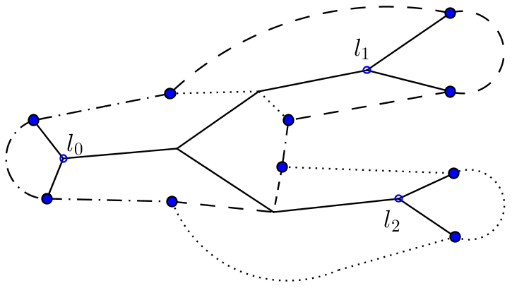
Figure 4: Illustration of $C(T)$. The dashed cycle is $C_{P}$ for $P$ from $l_{0}$ to $l_{1}$ and the dotted cycle is $C_{P^{\prime}}$ for $P^{\prime}$ from $l_{0}$ to $l_{2}$. The outer boundary forms $C(T)$.

Property (b)

We prove the following lemma and Property (b) follows from $C(T)=C^{|{\cal P}|}$.

Lemma 27.

$C^{i}$ strictly encloses only the vertices of $\bigcup_{j\leq i}P_{j}$ and encloses fewest faces.

Proof.

We prove this lemma by induction by assuming the lemma is true for $C^{i-1}$. The base case ($C^{1}$) follows from Lemma 25. Refer to Figure 5 (a). Since all the paths in $\cal P$ share the root $r$ of $T^{*}$ as one endpoint, $C^{i-1}$ and $C_{P_{i}}$ both strictly enclose $r$ and so must enclose a disk enclosing $r$. This disk is bounded by a cycle $C$ consisting of four subpaths: two vertex-disjoint subpaths $R_{1}$ and $R_{2}$ of $C^{i-1}\cap C_{P_{i}}$ and subpaths $R_{3}\subseteq C^{i-1}$ and $R_{4}\subseteq C_{P_{i}}$ each connecting $R_{1}$ and $R_{2}$.

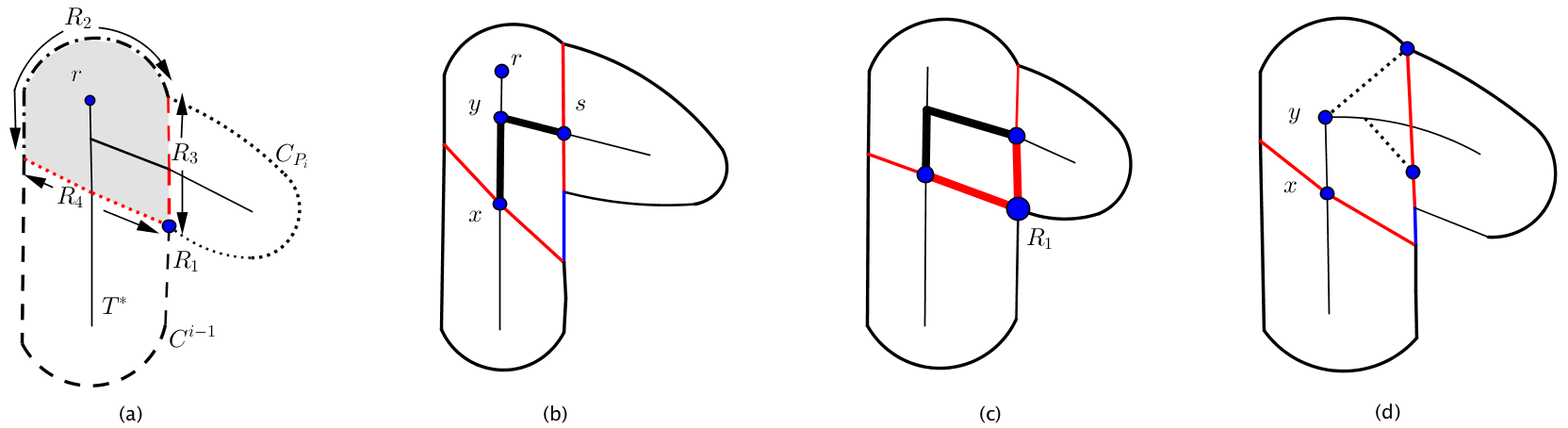
Figure 5: Examples for Lemma 27. (a) The dotted cycle is $C_{P_{i}}$ and the dashed cycle is $C^{i-1}$. The two red paths are $R_{3}$ and $R_{4}$. $R_{1}$ is trivial. The shaded region represents the common faces enclosed by $C^{i-1}$ and $C_{P_{i}}$. (b) The bold path is $P^{*}$ and $y$ is strictly inside of $C$. (c) If $R_{1}$ is a vertex, then the bold cycle only contains one terminal: $R_{1}$, which has two neighbors in $\bigcup_{j\leq i}P_{j}$. (d) The dotted paths represent possible $y$-to-$R_{3}$ paths inside of $C$ that is different from $P_{i}$.

Notice that $R_{3}$ must be enclosed by $C_{P_{i}}$ and contains a vertex of $T^{*}$, since $C^{i-1}$ strictly encloses only $\bigcup_{j<i}P_{j}$ and so is crossed by $P_{i}$ at some vertex in $R_{3}$. Similarly, $R_{4}$ must be enclosed by $C^{i-1}$ and contains a vertex in $T^{*}$. So there is an $R_{4}$-to-$R_{3}$ path $P^{*}$ in $\bigcup_{j\leq i}P_{j}$ enclosed by $C$. Let $xy$ be the first edge in $P^{*}$ with $x\in R_{4}$ (Figure 5 (b)). Then we have the following observations about $xy$:

Observation 4.

Edge $xy$ is nonremovable (since neither $x$ nor $y$ are terminals, Lemma 16).

Observation 5.

Vertex $y$ is strictly enclosed by $C$.

Proof.

Let $s$ be the endpoint of $P^{*}$ in $R_{3}$. Then $s\in P_{i}$ since $s$ is an internal vertex of $R_{3}$ and strictly enclosed by $C_{P_{i}}$. The $r$-to-$s$ path $\Psi_{1}$ of $T^{*}$ is strictly enclosed by $C_{P_{i}}$, so $\Psi_{1}$ is a subpath of $P_{i}$. The $r$-to-$x$ path $\Psi_{2}$ of $T^{*}$ is strictly enclosed by $C^{i-1}$, so $\Psi_{2}$ is a subpath of $\bigcup_{j<i}P_{j}$. Note the lowest common ancestor $LCA_{T^{*}}(x,s)$ of $x$ and $s$ in $T^{*}$ is in $\Psi_{1}\cap\Psi_{2}$. So $LCA_{T^{*}}(x,s)\neq x$ since $LCA_{T^{*}}(x,s)\in\Psi_{1}\subseteq P_{i}$ and $LCA_{T^{*}}(x,s)\neq s$ since $LCA_{T^{*}}(x,s)\in\Psi_{2}\subseteq\bigcup_{j<i}P_{j}$. See Figure 5 (b). It follows $LCA_{T^{*}}(x,s)$ is strictly enclosed by $C$. Since $y$ is between $x$ and $LCA_{T^{*}}(x,s)$ in $P^{*}$, we know $y\notin R_{3}$ and the claim follows. ∎

We argue that $R_{1}$ and $R_{2}$ must each contain at least one edge and so it will follow that $R_{3}$ and $R_{4}$ are vertex-disjoint. For a contradiction, assume $R_{1}$ is a vertex. Refer to Figure 5 (c). Consider the cycle $C^{*}$ formed by $\bigcup_{j\leq i}P_{j}$, a subpath of $R_{3}$, $R_{1}$ and a subpath of $R_{4}$. By Theorem 18, $C^{*}$ must contain a terminal. By construction, any terminal in $C^{*}$ must be in $R_{1}$. So $R_{1}$ is a terminal $t$. Since $t$ is the crossing of $C^{i-1}$ and $C_{P_{i}}$, $t$’s degree is at least four. By Lemma 19, there is an edge in $C$ incident to $t$ that is removable, which contradicts the minimality of $H$. The same argument holds for $R_{2}$. By the same reasoning, we have the following observation.

Observation 6.

Any vertex in $(C^{i-1}\cup C_{P_{i}})\setminus\bigcup_{j\leq i}P_{j}$ has at most one neighbor in $\bigcup_{j\leq i}P_{i}$.

Next, we will prove by contradiction that the subpath $S=C_{P_{i}}\setminus E(\bigcup_{j}R_{j})$ only shares endpoints with $C^{i-1}$. This will imply that $C^{i}$ strictly encloses only vertices of $P_{i}$ and vertices strictly inside of $C^{i-1}$. Further, this will also imply that $C^{i}$ encloses fewest faces. If there is another cycle $C^{I}$ that strictly encloses all vertices of $\bigcup_{j\leq i}P_{j}$ and fewer faces than $C^{i}$, then there is some face that is enclosed by $C^{i}$ but not enclosed by $C^{I}$. If that face is inside of $C^{i-1}$, then $C^{i-1}$ is not the cycle that encloses $\bigcup_{j<i}P_{j}$ and fewest faces, contradicting our inductive hypothesis; if that face is inside of $C_{P_{i}}$, then $C_{P_{i}}$ is not the cycle that encloses $P_{i}$ and fewest face, contradicting our choice of $C_{P_{i}}$. So there can not be such cycle $C^{I}$, giving the lemma.

To prove that $S$ only shares endpoints with $C^{i-1}$, we first have some claims.

Claim 28.

The $y$-to-$R_{3}$ subpath of $P_{i}$ is the only one $y$-to-$R_{3}$ path whose edges are strictly enclosed by $C$.

Proof.

By Observation 5, $y$ is strictly enclosed by $C$. For a contradiction, assume there is another $y$-to-$R_{3}$ path $\Psi$ enclosed by $C$ that is not a subpath of $P_{i}$. Notice that the endpoint of $\Psi$ in $R_{3}$ can not be an endpoint of $R_{3}$, for otherwise this endpoint of $R_{3}$ has two neighbors in $\bigcup_{j\leq i}P_{j}$, contradicting Observation 6. Then we know $\Psi\subseteq T^{*}$, and we have two $y$-to-$R_{3}$ paths in $T^{*}$, which together with $R_{3}$ form a cycle without any terminals, contradicting Theorem 18. See Figure 5 (d). ∎

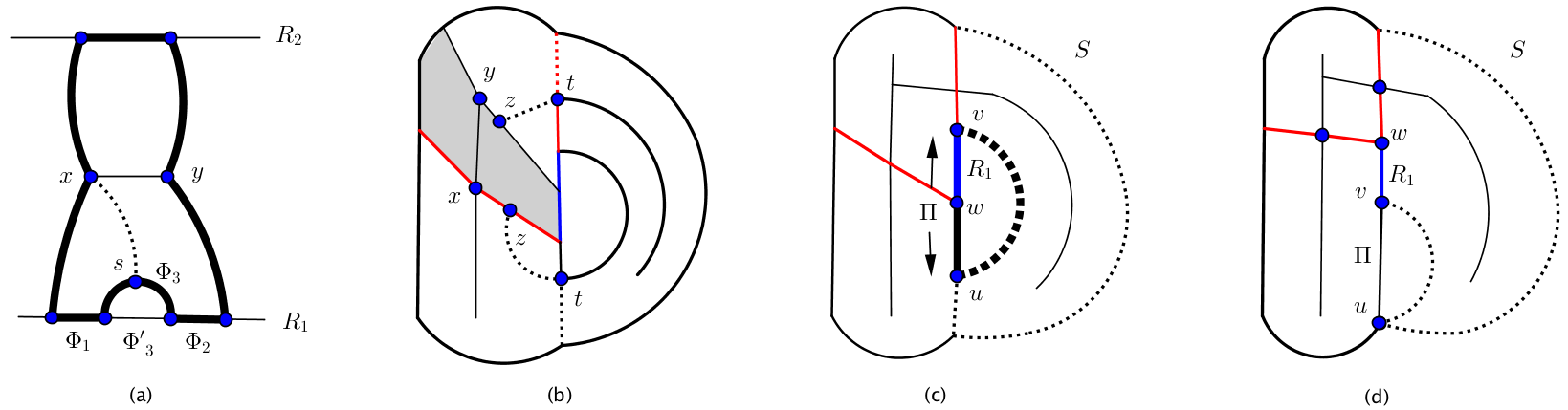
Figure 6: Examples for Lemma 27. (a) The bold cycle is $C(xy)$. (b) $C(xy)$ bounds the shaded region contains. The dotted paths are some possible examples for $\Phi$. (c) The dotted path is $S$, which shares a subpath with $C^{i-1}$. The bold cycle is $C^{\prime}$. $R_{3}$ and $R_{4}$ are disjoint. $\Pi$ contains $R_{1}$. (d) $\Pi$ does not contain $R_{1}$, and the endpoint $w$ of $R_{1}$ has two neighbors in $\bigcup_{j\leq i}P_{j}$.

Claim 29.

$C(xy)$ consists of two vertex-disjoint $R_{1}$-to-$R_{2}$ paths, a subpath of $R_{1}$ and a subpath of $R_{2}$.

Proof.

We show the two $x$-to-$y$ subpaths of $C(xy)$ share at least an edge with $R_{1}$ and $R_{2}$ respectively, that implies $C(xy)$ must contain two disjoint $R_{1}$-to-$R_{2}$ paths: one through $x$ and the other through $y$.

We first argue that the two $x$-to-$y$ paths in $C(xy)$ must each contain at least one terminal in $R_{1}\cup R_{2}$. $C(xy)\cup xy$ contains two cycles whose intersection is $xy$. By Theorem 18, each of these cycles must contain a terminal. Since neither $x$ nor $y$ are terminals, each of the $x$-to-$y$ paths in $C(xy)$ must contain a terminal. Note that $C(xy)$ is enclosed by $C$ and there is no terminal strictly enclosed by $C$. Further, since $R_{3}$ is enclosed by $C_{P_{i}}$, all its internal vertices are not terminals. Similarly, all internal vertices of $R_{4}$ are not terminals. So all the terminals in $C$ are either in $R_{1}$ or $R_{2}$, and each $x$-to-$y$ path in $C(xy)$ contains at least one terminal in $R_{1}\cup R_{2}$.

Next, we show the two terminals can not be both in $R_{1}$ or $R_{2}$, which implies the two paths must share vertices with $R_{1}$ and $R_{2}$ respectively. Notice that $P^{*}$ divides the region inside of $C$ into two parts, each of which has $R_{1}$ and $R_{2}$ in the bounding cycle respectively. If $C(xy)$ only contains vertices in $R_{1}$ or $R_{2}$, then $C(xy)$ must cross $P^{*}$ and there is another cycle that encloses $xy$ and fewer faces than $C(xy)$, contradicting the definition of $C(xy)$. Then $C(xy)$ must contain two $R_{1}$-to-$R_{2}$ paths: one through $x$ and the other through $y$.

Both of $C(xy)\cap R_{1}$ and $C(xy)\cap R_{2}$ can not be a vertex, for otherwise the vertex has two neighbors in $\bigcup_{j\leq i}P_{j}$, contradicting Observation 6. So the two $R_{1}$-to-$R_{2}$ paths are vertex disjoint.

We then argue that $C(xy)$ could only share one subpath with $R_{1}$, and the same argument holds for $R_{2}$. For a contradiction, assume there are more than one subpath of $C(xy)$ in $R_{1}$. Then let $\Phi_{1}$ and $\Phi_{2}$ be two such subpaths that are connected by a subpath $\Phi_{3}$ of $C(xy)$ that is not in $R_{1}$. Refer to Figure 6 (a). Notice that $\Phi_{3}$ is enclosed by a cycle $C^{\prime}$ consisting of $R_{1}$, an $x$-to-$R_{1}$ subpath of $C(xy)$, an $y$-to-$R_{1}$ subpath of $C(xy)$ and edge $xy$. Let $\Phi^{\prime}_{3}$ be the subpath of $R_{1}$ that has the same endpoints as $\Phi_{3}$. If $\Phi_{3}$ is an edge, then $(C^{i-1}\cup\Phi_{3})\setminus\Phi^{\prime}_{3}$ is a cycle that strictly encloses $\bigcup_{j<i}P_{j}$ and fewer faces than $C^{i-1}$, contradicting our inductive hypothesis. If $\Phi_{3}$ contains an internal vertex $s$, then $s\in\bigcup_{j<i}P_{j}$ since it is strictly enclosed by $C^{i-1}$. So there is an $s$-to-$x$ path in $\bigcup_{j<i}P_{j}$ whose edges must be enclosed by $C^{\prime}$. And then by replacing the $x$-to-$R_{1}$ subpath of $C(xy)$ with the $s$-to-$x$ path, we obtain a cycle that encloses $xy$ and fewer faces than $C(xy)$, contradicting the definition of $C(xy)$. ∎

Claim 30.

For every neighbor $z$ of $xy$ in $C(xy)\setminus\{R_{1},R_{2}\}$, there is a $z$-to-$(C^{i}\cup R_{1})$ path that shares only $z$ with $C(xy)$.

Proof.

If any neighbor $z$ of $xy$ in $C(xy)$ is not in $R_{1}\cup R_{2}$, then $z$ must be on an $R_{1}$-to-$R_{2}$ subpath of $C(xy)$, whose internal vertices are in $\bigcup_{j\leq i}P_{j}$. We construct a $z$-to-$(C^{i}\cup R_{1})$ path $\Phi$ as follows: first find a $z$-to-$C^{i-1}$ subpath $\Phi_{1}$ through $\bigcup_{j<i}P_{j}$, and then find a subpath $\Phi_{2}$ of $C^{i-1}$ that connects $\Phi_{1}$ with $C^{i}\cup R_{1}$ and is disjoint with $C(xy)$. Let $t$ be the endpoint of $\Phi_{1}$ in $C^{i-1}$. If $z\in C^{i-1}$, then $\Phi_{1}$ is empty and $t=z$. If $t\in C^{i}\cup R_{1}$, then $\Phi_{2}$ is empty. We define $\Phi=\Phi_{1}\cup\Phi_{2}$. In the following, we first argue that if $\Phi_{1}$ is not empty then it only shares $z$ with $C(xy)$, and then show that if $\Phi_{2}$ is not empty, then $\Phi$ only shares $z$ with $C(xy)$.

Assume $\Phi_{1}$ is not empty. Since $H$ is triconnected and $C(xy)$ encloses fewest faces, there exists a path $\Phi_{1}$ from $z$ to $C^{i-1}$ that is outside of $C(xy)$. Since $(\Phi_{1}\setminus\{t\})\subseteq\bigcup_{j<i}P_{j}$, $\Phi_{1}$ can not share any internal vertex with $C(xy)$. Further, $\Phi_{1}$ and $C(xy)$ can not share $t$, for otherwise $t$ will be an endpoint of $C(xy)\cap R_{1}$ or $C(xy)\cap R_{2}$ and it has two neighbors in $\bigcup_{j\leq i}P_{j}$: one via $\Phi_{1}$ and the other via $C(xy)$, contradicting Observation 6. So $\Phi_{1}$ only shares $z$ with $C(xy)$.

Consider the possible position of $t$ in $C^{i-1}$. If it is in $C^{i}\cup R_{1}$, then $\Phi_{2}$ is empty. If not, then it will be strictly enclosed by $C^{i}$. Refer to Figure 6 (b). There are two cases.

Case 1.

If $t$ is in $R_{3}$, then we choose as $\Phi_{2}$ a subpath of $R_{3}$.

Note that in this case $z$ could only be $y$’s neighbor by planarity and Claim 29. Consider the position of $z$.

If $z\notin R_{3}$, we argue $R_{3}$ and $C(xy)$ are vertex-disjoint, which will imply that there always exists a $t$-to-$C^{i}$ subpath of $R_{3}$. For a contradiction, assume $R_{3}$ and $C(xy)$ are not disjoint. Then $C(xy)$ must contains a $y$-to-$R_{3}$ subpath by planarity. Further, $\{yz\}\cup\Phi_{1}$ witnesses another $y$-to-$R_{3}$ path whose edges are strictly enclosed by $C$, contradicting Claim 28. So $R_{3}$ and $C(xy)$ are vertex-disjoint.

If $z\in R_{3}$, we argue $R_{3}$ contains a $z$-to-$(C^{i}\cup R_{1})$ subpath, which shares only $z$ with $C(xy)$. By Claim 29, $C(xy)$ contains two $R_{1}$-to-$R_{2}$ paths, one of which contains $y$. Then there are two $y$-to-$C$ subpaths of $C(xy)$: an $y$-to-$R_{1}$ subpath and an $y$-to-$R_{2}$ subpath, which are in distinct regions divided by $P^{*}$ and enclosed by $C$. By Claim 28, there is only one $y$-to-$R_{3}$ path whose edges are strictly enclosed by $C$. So only one of the $y$-to-$C$ subpath of $C(xy)$ shares vertices with $R_{3}$, and the other one is vertex-disjoint with $R_{3}$. If the $y$-to-$R_{i}$ subpath is disjoint with $R_{3}$ for $i=1$ or $i=2$, then there is a $z$-to-$R_{i}$ subpath of $R_{3}$ that shares only $z$ with $C(xy)$. Since $R_{2}\subseteq C^{i}$, we have the $z$-to-$(C^{i}\cup R_{1})$ subpath of $R_{3}$ that shares only $z$ with $C(xy)$.

Case 2.

If $t$ is not in $R_{3}$, then we choose as $\Phi_{2}$ the $t$-to-$C^{i}$ subpath of $C^{i-1}$ that is enclosed in $C^{i}$. This subpath always exists and is disjoint with $C(xy)$.

∎

Now we prove that $S$ only shares endpoints with $C^{i-1}$. For a contradiction, assume $S$ has an internal vertex that is in $C^{i-1}$. Then by construction $C^{i}$ would enclose either $R_{1}$ or $R_{2}$; w.l.o.g. assume $R_{1}$ is enclosed by $C^{i}$. Let $\Pi$ be the minimal subpath of $C^{i-1}$ that is enclosed by $C^{i}$ and connects an internal vertex $u$ of $S$ with the common endpoint $v$ of $R_{1}$ and $S$. Let $w$ be the other endpoint of $R_{1}$. There is a simple cycle $C^{\prime}$ consisting of two $u$-to-$v$ subpaths: one is $\Pi$ and the other is a subpath of $S$. See Figure 6 (c). Further, $\Pi$, and also $C^{\prime}$, contains $R_{1}$, for otherwise $R_{3}$ and $R_{4}$ share $w$ as an endpoint and $w$ has two neighbors in $\bigcup_{j\leq i}P_{j}$: one via $R_{3}$ and the other via $R_{4}$, contradicting Observation 6. See Figure 6 (d). It follows that $R_{3}$ and $R_{4}$ are vertex disjoint $C^{\prime}$-to-$C^{i}$ paths.

We argue $H$ and $xy$ satisfy the conditions of Lemma 26 with $C_{1}=C^{\prime}$ and $C_{2}=C^{i}$, which shows $xy$ is removable, giving a contradiction to Observation 4:

Condition 1.

Note that $C_{1}$ and $C_{2}$ could only share at most one vertex which is $u$ and shown in Figure 6 (d). Since $C_{P_{i}}$ is simple, $u\neq w$, so $u\notin C$. Since $C(xy)$ is enclosed by $C$, $u\notin C(xy)$. So $C(xy)$ does not contain the common vertex of $C_{1}$ and $C_{2}$. Then the first condition in Lemma 26 follows from Claim 29.

Condition 2.

Since $R_{1}\subseteq C_{1}$, the second condition follows from Claim 30. Note that the $z$-to-$C^{i}$ path $\Phi$ constructed in Claim 30 may contain a $z$-to-$C_{1}$ subpath, which shares only $z$ with $C(xy)$.

∎

$T$ is a tree

To prove this, we show that when $T$ is a tree, $H$ is $Q_{3}$-triconnected. That is, for any pair of terminals $x$ and $y$, there are three $x$-to-$y$ internally vertex-disjoint paths only one of which contains internal vertices of $T$ when $T$ is a tree. Since $T$ is connected, this implies $T$ can not contain any cycle, for otherwise $H$ is not minimal. The proof is similar to that of Lemma 21 but simpler: we modify the paths between $x$ and $y$ such that only one of them contains internal vertices of $T$ while maintaining them internally vertex-disjoint.

Let $R_{1},R_{2}$ and $R_{3}$ be three $x$-to-$y$ disjoint paths. If there is only one path containing internal vertices of $T$, then it is sufficient for $T$ to be simply connected for triconnectivity between $x$ and $y$. So we assume there are at least two paths containing internal vertices of $T$. By Lemma 27, $C(T)$ strictly encloses all internal vertices of $T$, so any path that contains an internal vertex of $T$ must touch $C(T)$. We order the vertices of the three paths from $x$ to $y$. Let $u_{i}$ and $v_{i}$ be the first and last vertex of $R_{i}$ that is in $C(T)$ for $i=1,2,3$. If $R_{i}$ is disjoint from $C(T)$, we say $u_{i}$ and $v_{i}$ is undefined. Let $C_{1}$ and $C_{2}$ be the disjoint minimum paths of $C(T)$ that connect $\{u_{1},u_{2},u_{3}\}$ and $\{v_{1},v_{2},v_{3}\}$. If there are only two paths, say $R_{1}$ and $R_{2}$, containing vertices of $C(T)$, we can replace $R_{1}[u_{1},v_{1}]\cup R_{2}[u_{2},v_{2}]$ with $C_{1}\cup C_{2}$. Then the new paths are disjoint and do not contain any internal vertex of $T$. If all the three paths contain vertices of $C(T)$, then let $C_{3}$ be the simple path from the middle vertex of $\{u_{1},u_{2},u_{3}\}$ to the middle vertex of $\{v_{1},v_{2},v_{3}\}$ in $(C(T)\cup T)\setminus(C_{1}\cup C_{2})$. Now the to-$C(T)$ prefices of $R_{i}$, $C_{i}$ and the from-$C(T)$ suffices of $R_{i}$ (for $i=1,2,3$) together form three vertex-disjoint paths between $x$ and $y$. Further, among the three resulting paths, only the path containing $C_{3}$ contains internal vertices of $T$. Therefore, it is sufficient for $T$ to be simply connected for $H$ to be $Q_{3}$-triconnected.

Property (c)

By triconnectivity, every leaf of $T^{*}$ has at least two neighbors on $T$ that are terminals. So each leaf of $T^{*}$ can not be a leaf of $T$ and then all leaves of $T$ are terminals. By Lemma 27, $C(T)$ only strictly encloses all vertices of $T^{*}$. So all its neighbors, which are terminals in $T$ by the maximality of $T^{*}$, are on $C(T)$, giving property (c).

Since each terminal-bounded component is a tree, any terminal on $T$ must be a leaf by the construction of terminal-bounded component. Therefore, we have the following lemma.

Lemma 31.

A vertex of a terminal-bounded tree $T$ is a terminal if and only if it is a leaf of $T$.

Property (d)

Let $T_{1}$ be any terminal-bounded tree. For a contradiction, assume there is a terminal-bounded tree $T_{2}$ whose vertices are in distinct maximal terminal-free paths of $C(T_{1})$. By Lemma 31, the leaves of $T_{2}$ are terminals. So each component of $C(T_{1})\cap T_{2}$ is a terminal-to-terminal path and contains at most one maximal terminal-free path. Then by the assumption for the contradiction, there are two vertex-disjoint non-trivial components (paths) $\Pi_{1}$ and $\Pi_{2}$ of $C(T_{1})\cap T_{2}$.

Since $C(T_{2})$ strictly encloses only internal vertices of $T_{2}$, the interiors of $C(T_{2})$ and $C(T_{1})$ overlap, and so $C(T_{2})\cap T_{1}\neq\emptyset$. Then $C(T_{2})\cap T_{1}$ contains only paths whose endpoints are terminals on $C(T_{1})$. Let $\cal R$ be the set consisting of all maximal paths of $C(T_{2})\cap T_{1}$. Refer to Figure 7 (a) and (b). Since $C(T_{2})$ is simple, and since the endpoints of paths in $\cal R$ are leaves of $T_{1}$, we have

Observation 7.

Any two paths in $\cal R$ are vertex disjoint.

Note that if $T_{1}$ is an edge or a star, $|{\cal R}|\leq 1$ and so we would already have our contradiction.

For any path $R_{i}\in\cal R$ with endpoints $u_{i}$ and $v_{i}$, there is an $u_{i}$-to-$v_{i}$ subpath $R^{\prime}_{i}$ of $C(T_{1})$ such that $R_{i}$ and $R^{\prime}_{i}$ form a cycle enclosing a region that is enclosed by both of $C(T_{1})$ and $C(T_{2})$. Since $C(T_{1})$ and $C(T_{2})$ only strictly enclose edges of $T_{1}$ and $T_{2}$ respectively, and since $T_{1}\neq T_{2}$, this region must be a face. Notice that any path of $C(T_{1})\cap T_{2}$ could only be subpath of $R^{\prime}_{i}$ for some $R_{i}\in\cal R$ for $C(T_{2})$ encloses $T_{2}$. By the following observation, there exist $R_{1}$ and $R_{2}$ such that $\Pi_{1}\subseteq R^{\prime}_{1}$ and $\Pi_{2}\subseteq R^{\prime}_{2}$.

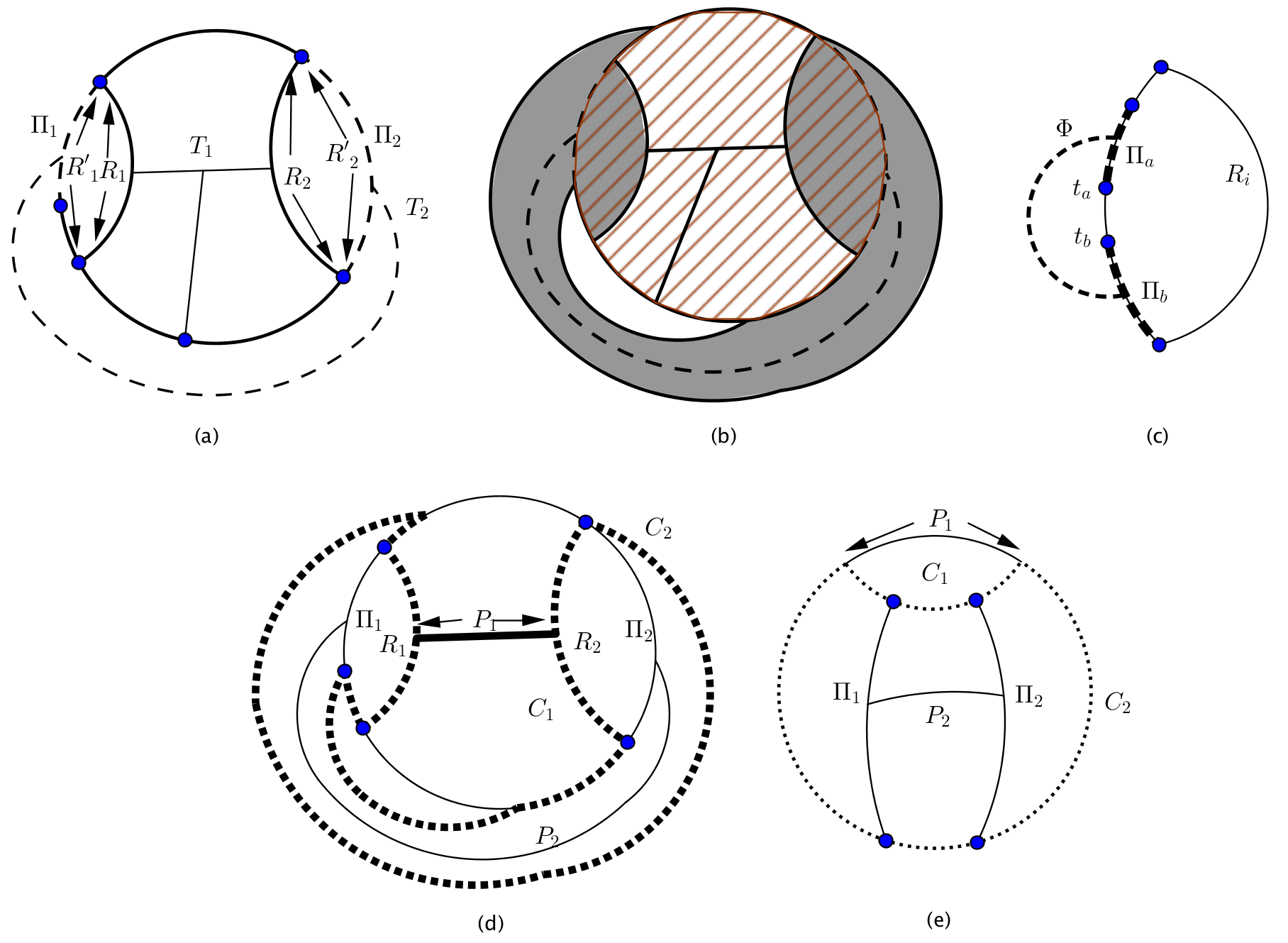
Figure 7: (a) The dashed tree is $T_{2}$ and there are two paths $\Pi_{1}$ and $\Pi_{2}$ of $T_{2}$ on $C(T_{1})$. The blue vertices are terminals. (b) The two shaded cycles are $(T_{1})$ and $C(T_{2})$, which shares two regions enclosed by $R_{i}$ and $R^{\prime}_{i}$ for $i=1,2$. (c) The dashed subtree is in $T_{2}$. $R^{\prime}_{i}$ contains two subpaths of $T_{2}$ and two terminals $t_{a}$ and $t_{b}$ are enclosed. (d) The dotted cycle is $C(T_{2})$. The bold cycles $C_{1}$ and $C_{2}$ share $P_{1}$. (e) An example for Simplified $C_{1}$ and $C_{2}$ in (d). The dotted cycle is $C(T_{2})$ and the outer cycle is $C_{2}$. $C_{1}$ and $C_{2}$ share $P_{1}$.

Observation 8.

Every $R^{\prime}_{i}$ contains at most one maximal path of $T_{2}$.

Proof.

For a contradiction, assume there is a path $R^{\prime}_{i}$ that contains more than one maximal path of $T_{2}$. Let $\Pi_{a}$ and $\Pi_{b}$ be two successive such paths. By the concept of terminal-bounded tree, there is a terminal-free path $\Phi$ of $T_{2}$ connecting $\Pi_{a}$ with $\Pi_{b}$ that only share endpoints with $C(T_{1})$. Refer to Figure 7 (c). So $\Phi$, $R_{i}$ and $R^{\prime}_{i}$ (which contains two $R_{i}$-to-$\Phi$ paths) witness a cycle $C$ that strictly encloses an endpoint $t_{a}$ of $\Pi_{a}$ and an endpoint $t_{b}$ of $\Pi_{b}$. Since the endpoints of $\Pi_{a}$ and $\Pi_{b}$ are leaves of $T_{2}$, $t_{a}$ and $t_{b}$ should be in $C(T_{2})$ by Property (c). So there is a subpath $P$ of $C(T_{2})$ that is enclosed by $C$ such that $t_{a}\in P$. Since the region enclosed by $C$ is divided into two parts by a subpath $\Phi^{\prime}$ of $R^{\prime}_{i}$ (which have the same endpoints as $\Phi$), and since one of the two parts is the face enclosed by $R_{i}$ and $R^{\prime}_{i}$, we know $P$ could only be in the region bounded by $\Phi^{\prime}$ and $\Phi$. However, $P$ can not cross $\Phi$ by Property (a) since $\Phi$ is terminal-free and every vertex of $\Phi$ is an internal vertex of $T_{2}$; and $P$ can not cross any internal vertex of $\Phi^{\prime}$ for otherwise $P$ will enter the face enclosed by $R_{i}$ and $R^{\prime}_{i}$. Therefore, $P$ and $R_{i}$ can not be connected, contradicting $P$ is a subpath of $C(T_{2})$. ∎

Next, we construct two cycles $C_{1}$ and $C_{2}$ that share a subpath. Refer to Figure 7 (d). Since $T_{1}$ is a tree and $R_{1}$ and $R_{2}$ are vertex disjoint by Observation 7, there is an $R_{1}$-to-$R_{2}$ subpath $P_{1}$ in $T_{1}$. Since $C(T_{2})$ is simple and contains $R_{1}$ and $R_{2}$, $C(T_{1})\cup P_{1}$ contains two simple cycles $C_{1}$ and $C_{2}$ whose intersection is $P_{1}$. W.l.o.g. assume $C_{1}$ is enclosed by $C_{2}$.

Since $T_{2}$ is a tree and $\Pi_{1}$ and $\Pi_{2}$ are vertex disjoint, there is a $\Pi_{1}$-to-$\Pi_{2}$ path $P_{2}$ in $T_{2}$. Note that $P_{2}$ is terminal-free, since $P_{2}$ does not contain any leaf of $T_{2}$ and terminals in $T_{2}$ are leaves by Lemma 31. Let $xy$ be an edge of $P_{2}$. Then by Lemma 16, $xy$ is nonremovable. However, $H$ and $xy$ also satisfy Lemma 26 with $C_{1}$ and $C_{2}$, which shows $xy$ is removable, giving a contradiction.

Condition 1.

Note that $C(xy)$ is enclosed by the cycle $C$ consisting of $\Pi_{1}$, $\Pi_{2}$, and two $\Pi_{1}$-to-$\Pi_{2}$ subpaths of $C(T_{2})$: one is of $C_{1}$ and the other is of $C_{2}$. Refer to Figure 7 (d) and (e). Since $C$ is disjoint with the common subpath $P_{1}$ of $C_{1}$ and $C_{2}$, $C(xy)$ is also disjoint with $P_{1}$.

Showing the remainder of the first condition of Lemma 26 is similar to that of Claim 29 if we replace $R_{1}$ and $R_{2}$ with the two $\Pi_{1}$-to-$\Pi_{2}$ subpaths of $C_{1}$ and $C_{2}$. Note that we have a stronger version of Observation 6 here, since $T_{2}$ is a tree.

Condition 2.

If any neighbor $z$ of $xy$ in $C(xy)$ is not in $C_{1}\cup C_{2}$, it will be a non-leaf vertex in $T_{2}$, since all leaves of $T_{2}$ are in $C(T_{2})\subseteq C_{1}\cup C_{2}$. Then $z$ is not a terminal by Lemma 31. We find a subpath $\Phi$ in $T_{2}$ from $z$ to $C(T_{2})\subseteq C_{1}\cup C_{2}$ such that $\Phi$ only shares $z$ with $C(xy)$. By triconnectivity, there are at least three disjoint paths from $z$ to $C(T_{2})$. Since $C(xy)$ contains two such paths and encloses the fewest faces, there is a path $\Phi$ from $z$ to $C(T_{2})$ outside of $C(xy)$. If $\Phi$ shares any vertex with $C(xy)$ other than $z$, then $\Phi$ and the $C_{1}$-to-$C_{2}$ path that contains $z$ witness a cycle in $T_{2}$, a contradiction.

This proves the Tree Cycle Theorem.

3.2.1 Terminal-free paths

Let $P$ be a terminal-free $a$-to-$b$ path of $H$ such that there exists a cycle that strictly encloses the internal vertices of $P$. Then $a,b\in C(P)$, since $H$ is triconnected by Lemma 12. Let $P_{1}(P)$ and $P_{2}(P)$ be the two $a$-to-$b$ subpaths of $C(P)$.

Lemma 32.

If for every edge $e\in P$ there is a separating set $S_{e}\in C(P)$, then all the vertices inside of $C(P)$ are in $P$.

Proof.

For a contradiction, assume there is a vertex $u$ strictly inside of $C(P)$ that is not on $P$. There can not be more than one path from $u$ to $C(P)$ disjoint from $P$, otherwise there will be another cycle which encloses fewer faces than $C(P)$ (Figure 8 (a)). By Lemma 12, $H$ is triconnected, so there are at least two disjoint paths $R_{1}$ and $R_{2}$ from $u$ to $v_{1}$ and $v_{2}$ on $P$ disjoint from $C(P)$ (Figure 8 (b)). For an edge $e$ on $P$ between $v_{1}$ and $v_{2}$, every separating set for $e$ must include a vertex on the path $R_{1}\cup R_{2}$, however, this contradicts the assumption that there is a separating set for $e$ in $C(P)$.

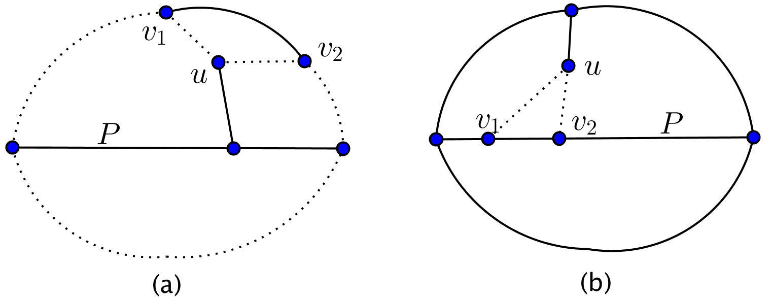
Figure 8: (a) If vertex $u$ has two paths to $v_{1}$ and $v_{2}$ on $C(P)$ that are disjoint from $P$, then there is a smaller cycle (dotted) through $v_{1},u,v_{2}$ that encloses $P$. (b) The separating set for an edge $e$ on $P$ between $v_{1}$ and $v_{2}$ must include a vertex of the path (dotted) strictly enclosed by $C(P)$, contradicting there is a separating set for $e$ in $C(P)$.

∎

Lemma 33.

No pair of adjacent vertices in $P$ has a common neighbor in $C(P)$.

Proof.

For a contradiction, assume there are adjacent vertices $u$ and $v$ with a common neighbor $z$ in $C(P)$. Since $u,v,z$ forms a cycle, $S_{uv}$ must contain $z$. Therefore, by Theorem 10, $uz$ is removable. Further, both components of $H\setminus\{uv,S_{uv}\}$ must contain a vertex distinct from $u$ and $v$ and each of those vertices must have vertex disjoint paths to $S_{uv}$ and $uv$; therefore the degree of $z$ is at least 4. Therefore, removing $uz$ will not result in contracting any edges incident to $z$ and so will preserve triconnectivity of the terminals, contradicting the minimality of $H$. ∎

For a separating pair $(e,S_{e})$, let $\Sigma(e,S_{e})$ be a closed curve that only intersects the drawing of $H$ in an interior point of $e$ and two vertices of $S_{e}$ and partitions the plane according to the components of $H\setminus(\{e\}\cup S_{e})$. Each portion of $\Sigma(e,S_{e})\setminus H$ is contained in a face of $H$. Since this is true for any $\Sigma(e,S_{e})$, for two separating pairs $(e_{1},S_{e_{1}})$ and $(e_{2},S_{e_{2}})$ we may assume that the curves $\Sigma(e_{1},S_{e_{1}})$ and $\Sigma(e_{2},S_{e_{2}})$ are drawn so they cross each other at most 3 times. $\Sigma(e_{1},S_{e_{1}})$ and $\Sigma(e_{2},S_{e_{2}})$ cross either at a point that is interior to a face of $H$ or at one vertex of $S_{e_{1}}\cup S_{e_{2}}$. Since they are simple closed curves, they cross each other twice or not at all.

Lemma 34.

For every edge $e$ in $P$, there exists a separating set for $e$ in $C(P)$.

Proof.

We prove by induction on the subpaths of $P$: we assume the lemma is true for every strict subpath of $P$. The base case is when $P$ is one edge $xy$: $S_{xy}$ must include one vertex of $P_{1}(xy)$ and one vertex of $P_{2}(xy)$ but does not include $x$ or $y$, giving the lemma.

Let $xy$ be any edge of $P$. Without loss of generality, we assume $x\neq a$ and $y\notin P[a,x]$. By the inductive hypothesis, there exists a separating set $S_{xy}=\{s_{1},s_{2}\}$ in $C(P[x,b])$. The following claim simplifies our proof, which we prove after using this claim to prove that $S_{xy}\in C(P)$.

Claim 35.

$S_{xy}$ does not contain an internal vertex of $P$.

There are two cases:

1. If $b\in S_{xy}$, w.l.o.g. assume $b=s_{1}$. Then we only need to show $s_{2}$ is in $C(P)$. By the induction hypothesis, $s_{2}\in C(P[x,b])$. By Claim 35, $s_{2}$ can not be internal vertex of $P[a,y]$, so $a$ and $x$ must be in the same component of $H\setminus\{xy,S_{xy}\}$. Then $C(P[a,y])$ must contain $s_{2}$ since $C(P[a,y])$ must intersect $\Sigma(xy,S_{xy})$ in vertices of $S_{xy}$. Therefore, $s_{2}$ is in both of $C(P[a,y])$ and $C(P[x,b])$. By planarity, it must be in $C(P)$, for otherwise there will be other cycles which enclose fewer faces than $C(P[a,y])$ and $C(P[x,b])$ and do not contain $s_{2}$.

2. If $b\notin S_{xy}$, by Claim 35, $S_{xy}$ is not in $P$, so $a$ and $b$ are in the distinct components of $H\setminus\{xy,S_{xy}\}$ since they are connected to $x$ and $y$ by $P[a,x]$ and $P[y,b]$ respectively. That is, $b$ is strictly inside of $\Sigma(xy,S_{xy})$ and $a$ is outside of $\Sigma(xy,S_{xy})$. Then $C(P)$ must intersect $\Sigma(xy,S_{xy})$ twice in vertices of $S_{xy}$. Because $C(P)$ is simple, it can not intersect $\Sigma(xy,S_{xy})$ in the same vertex of $S_{xy}$. Therefore, both vertices of $S_{xy}$ are in $C(P)$.

This completes the proof of Lemma 34. ∎

Proof of Claim 35.

For a contradiction, assume $s_{1}$ is an internal vertex of $P$. Then it must in $P[a,x]$ since $S_{xy}$ is in $C(P[x,b])$. Further, $s_{2}$ can not be also in $P[a,x]$ since $x$ and $y$ are triconnected to $C(P)$, and then $C(P)$ and the paths from $x$ and $y$ to $C(P)$ contains a path from $x$ to $y$ disjoint from $P[a,x]$.

Since $a$ and $x$ are on different sides of $\Sigma(xy,S_{xy})$, $C(P[a,x])$ must cross $\Sigma(xy,S_{xy})$ twice. $\Sigma(xy,S_{xy})$ could only intersect $H$ at $xy$ and $S_{xy}$, so $C(P[a,x])$ must cross $\Sigma(xy,S_{xy})$ at $xy$ and $s_{2}$, for $s_{1}$ is in $P[a,x]$ and $C(P[a,x])$ is simple; w.l.o.g. assume $P_{1}(P[a,x])$ contains $s_{2}$.

In $P[s_{1},x]$, there must be a vertex between $s_{1}$ and $x$, for otherwise by Theorem 10 edge $s_{1}x$ is removable, which contradicts Lemma 16. Let $zx$ be an edge of $P[s_{1},x]$. Then there exists a separating set $S_{zx}$ for $zx$ in $C(P[a,x])$ by induction hypothesis. We claim $\Sigma(zx,S_{zx})$ must intersect $P_{1}(P[a,x])$ between $s_{2}$ and $x$. If not, then it will intersect $P_{1}(P[a,x])$ outside of $\Sigma(xy,S_{xy})$. However, the $z$-to-$s_{2}$ path, together with the $s_{2}$-to-$x$ subpath of $P_{1}(P[a,x])$ and edge $zx$ form a cycle inside of $\Sigma(xy,S_{xy})$. See Figure 9 (a). Since $\Sigma(zx,S_{zx})$ must cross the edge $zx$, it must intersect the described cycle twice. Note that cycle is disjoint from $P_{2}(P[a,x])$. So $\Sigma(zx,S_{zx})$ will intersect the drawing of $H$ four times: twice at the described cycle inside of $\Sigma(xy,S_{xy})$, once at $P_{1}(P[a,x])$ outside of $\Sigma(xy,S_{xy})$ and once at $P_{2}(P[a,x])$. This contradicts the definition of $\Sigma(zx,S_{zx})$. Let $s$ be the vertex of $S_{zx}$ in $P_{1}(P[a,x])$. By the above argument, $s$ is between $s_{2}$ and $x$. There are two cases.

1. If $s=s_{2}$, the only vertex of $P_{1}(P[a,x])$ inside both of $\Sigma(zx,S_{zx})$ and $\Sigma(xy,S_{xy})$ is $s_{2}$. Then there is a path between $z$ and $s_{2}$ edge disjoint from $C(P[a,x])$ and $P$. By Lemma 32, all vertices inside of $C(P[a,x])$ are in $P[a,x]$, so $z$ and $s_{2}$ are adjacent and this edge is the only path between $z$ and $s_{2}$ disjoint from $P$ in $\Sigma(xy,S_{xy})$. Consider $C(P[z,b])$. It must intersect $\Sigma(xy,S_{xy})$ at $s_{1}$ and $s_{2}$. Then edge $zs_{2}$ must be in $C(P[z,b])$ since it is the only path between $z$ and $s_{2}$ disjoint from $P$ in $\Sigma(xy,S_{xy})$. By Lemma 32, the $x$-to-$s_{2}$ path disjoint from $P$ in $\Sigma(xy,S_{xy})$ is an edge. However, the two edges $zs_{2}$ and $xs_{2}$ contradict Lemma 33.

2. If $s\neq s_{2}$, $S_{zx}$ must contain vertex $a$, for otherwise $\Sigma(zx,S_{zx})$ will intersect $P_{1}[a,x]$ between $a$ and $s_{2}$, which is the second intersection for $\Sigma(zx,S_{zx})$ and $P_{1}[a,x]$ and the fourth for $\Sigma(zx,S_{zx})$ and $H$. Then $s_{1}$ and $z$ are both connected to $s$ by paths edge disjoint from $C(P[a,x])$ and $P$ since they are inside of $\Sigma(zx,S_{zx})$. By Lemma 32 they are both adjacent to $s$. See Figure 9 (c). However, this contradicts Lemma 33. ∎

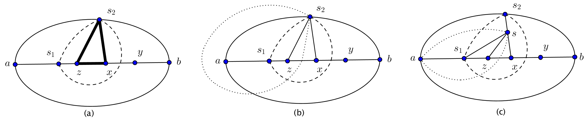
Figure 9: $\Sigma(xy,S_{xy})$ is the dashed cycle and $\Sigma(zx,S_{zx})$ is the dotted cycle. (a) The bold cycle must be intersected by $\Sigma(zx,S_{zx})$ twice. (b) $\Sigma(zx,S_{zx})$ intersects the drawing of $H$ at $s_{2}$. (c) $\Sigma(zx,S_{zx})$ intersects the drawing of $H$ at $s$ and $a$.

Lemma 36.

Let $u_{1}$ and $u_{2}$ be the neighbors of an endpoint of $P$ on $C(P)$. Then there is a $u_{1}$-to-$u_{2}$ path whose internal vertices are strictly outside of $C(P)$.

Proof.

Without loss of generality, let $u_{i}$ be the neighbor of $a$ on $P_{i}(P)$, $i=1,2$. Let $\{s_{1},s_{2}\}$ be the separating set for $ac\in P$ such that $s_{i}\in P_{i}(P)$, $i=1,2$, as guaranteed by Lemma 34.

If $u_{i}=s_{i}$, $i=1,2$, then the component of $H\setminus\{ac,s_{1},s_{2}\}$ that contains $a$ must contain another vertex $x$ and $x$ must have three vertex-disjoint paths to $a$, $s_{1}$ and $s_{2}$. The latter two of these witness the $u_{1}$-to-$u_{2}$ path that gives the lemma.

If $u_{1}\neq s_{1}$ and $u_{2}=s_{2}$, then the component of $H\setminus\{ac,s_{1},s_{2}\}$ that contains $u_{1}$ must have three vertex-disjoint paths to $a$, $s_{1}$ and $s_{2}$ and the latter of these paths witness the $u_{1}$-to-$u_{2}$ path that gives the lemma. The case $u_{1}=s_{1}$ and $u_{2}\neq s_{2}$ is symmetric.

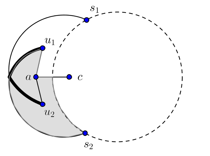
Figure 10: The construction of paths for Lemma 36. $\Sigma(ac,\{s_{1},s_{2}\})$ is the dashed cycle. The $u_{2}$ side of the cycle that separates $u_{2}$ and $s_{1}$ is shaded. The path witnessing the lemma is bold and is formed by the $u_{2}$-to-$s_{1}$ and $u_{1}$-to-$s_{2}$ paths that avoid edges $u_{1}a$ and $u_{2}a$.

If $u_{i}\neq s_{i}$, $i=1,2$, then the component of $H\setminus\{ac,s_{1},s_{2}\}$ that contains $u_{1}$ and $u_{2}$ must have three vertex-disjoint paths from $u_{i}$ to $a$, $s_{1}$ and $s_{2}$ for $i=1,2$. The first of these, we may assume is the edge $u_{i}a$. Consider the $u_{1}$-to-$s_{2}$ path; together with the edges $u_{1}a$ and $ac$ and the $s_{2}$-to-$ac$ portion of $\Sigma(ac,\{s_{1},s_{2}\})$ that does not contain $s_{1}$, these form a closed curve in the plane that separates $u_{2}$ and $s_{1}$ (see Figure 10). The above-described $u_{2}$-to-$s_{1}$ path must therefore cross the $u_{1}$-to-$s_{2}$ path; these paths witness the $u_{1}$-to-$u_{2}$ path that gives the lemma. ∎

Lemma 37.

For any terminal-free path $P$, there is a drawing of $H$ such that all internal vertices of $P$ are strictly enclosed by a simple cycle.

Proof.

For a contradiction, assume there is a terminal-free path $P$ whose internal vertices is not strictly enclosed by any cycle for any choice of infinite face of $H$: that is, every face of $H$ contains an internal vertex of $P$. Let $P$ be a minimal such path, let $a$ and $b$ be $P$’s endpoints, and let $c$ be $a$’s neighbor on $P$. Note that $b\neq c$, for otherwise $P$ is an edge and $H$ would have at most two faces (each containing $P$), but every triconnected graph has at least three faces.

First observe that there is a face $f$ whose bounding cycle strictly encloses all internal vertices of $P[c,b]$. Let $f_{1}$ and $f_{2}$ be the two faces that contains edge $ac$: $f$ is one of $f_{1}$ and $f_{2}$. One of $f_{1}$ and $f_{2}$ only contains one internal vertex, namely $c$, of $P$, for otherwise both faces would contain at least two internal vertices of $P$ and every face of $H$ would contain an internal vertex of $P[c,b]$, contradicting the minimality of $P$.

Take $f$, defined in the previous paragraph, to be the infinite face of $H$. Since $f$’s bounding cycle strictly encloses the internal vertices of $P[c,b]$, $C(P[c,b])$ exists. Let $u$ and $v$ be $c$’s neighbors in $C(P[c,b])$. Note that $ac$ may or may not be in $C(P[c,b])$. By Lemma 36, there is a $u$-to-$v$ path $R$ whose internal vertices are strictly outside of $C(P[c,b])$, so there is a drawing of $H$ so that $R\cup C(P[c,b])\setminus\{cu,cv\}$ is a cycle that strictly encloses internal vertices of $P$, a contradiction. See Figure 11 (a).

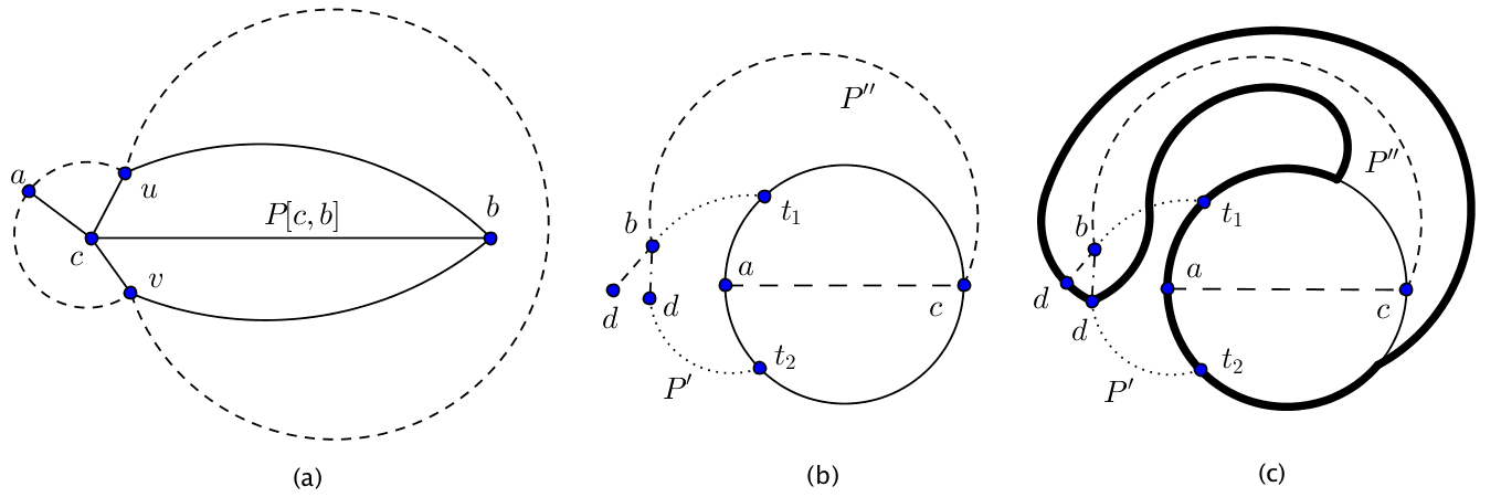
Figure 11: (a) The dashed paths show two possible $u$-to-$v$ paths $R$ outside of $C(P[c,b])$. The cycle $R\cup C(P[c,b])\setminus\{cu,cv\}$ strictly encloses a face that does not contain any internal vertex of $P$ for an appropriate choice of infinite face. (b) The dotted path is $P^{\prime}$ and dashed path is $P^{\prime\prime}$. Note that $d$ may or may not be in $P^{\prime}$. (c) The bold cycle is $C(P^{\prime\prime})$ and it crosses $P^{\prime}$.

∎

Proof of Lemma 24.

If $T^{*}$ is an edge, then this claim is trivial. Suppose otherwise.

For a contradiction, assume every face of $H$ contains an internal vertex of $T^{*}$. Let $ac$ be a leaf edge of $T^{*}$, where $a$ is a leaf of $T^{*}$. Recall that if a terminal-bounded component is not an edge, then it is obtained from a maximal terminal-free tree. By the maximality of $T^{*}$, the two neighbors, $t_{1}$ and $t_{2}$, of $a$ on $C(ac)$ are terminals. By Lemma 36, there exists a $t_{1}$-to-$t_{2}$ path $P^{\prime}$ whose internal vertices are strictly outside of $C(ac)$. Choose $P^{\prime}$ such that $C^{\prime}=P^{\prime}\cup\{at_{1},at_{2}\}$ encloses the fewest faces. Then $C^{\prime}$ does not strictly enclose any vertex since $H$ is triconnected by Lemma 12. By the assumption for the contradiction and the choice of $P^{\prime}$, $P^{\prime}$ must contain an internal vertex $b$ of $T^{*}$.

Let $P^{*}$ be the $a$-to-$d$ path of $T^{*}$ containing vertex $b$. Note that $d$ may or may not be in $P^{\prime}$ (see Figure 11 (b)). By Lemma 37, $C(P^{*})$ exists and by Lemmas 32 and 34, $C(P^{*})$ strictly encloses only internal vertices of $P^{*}$. Then $C^{\prime}$ and $C(P^{*})$ must cross each other and there exists a subpath of $C(P^{*})$ that is strictly enclosed by $C^{\prime}$, which contradicts that $C^{\prime}$ encloses fewest faces. See Figure 11 (c). ∎

Proof of Lemma 25.

By Lemma 37, $C(P)$ exists. Then $P_{1}(P)$ and $P_{2}(P)$ both contain a terminal, for otherwise there is a cycle composed by $P$ and one of $P_{1}(P)$ and $P_{2}(P)$ that does not contain any terminal, contradicting Theorem 18. We first prove that at least one of $P_{1}(P)$ and $P_{2}(P)$ contains more than one internal vertex, and then construct the cycle strictly enclosing $P$. By Lemma 32 and 34, all vertices inside of $C(P)$ are in $P$. If $P_{1}(P)$ and $P_{2}(P)$ both only contain one internal vertex, then the endpoints of the first edge of $P$ are both adjacent to the internal vertex of $P_{1}(P)$ or $P_{2}(P)$, which contradicts Lemma 33. Let $x_{a}$ and $y_{a}$ (or $x_{b}$ and $y_{b}$) be the neighbors of $a$ (or $b$) in $P_{1}(P)$ and $P_{2}(P)$ respectively. Then at least one of $\{x_{a},x_{b}\}$ and $\{y_{a},y_{b}\}$ contains two distinct vertices.

By Lemma 36, there is an $x_{a}$-to-$y_{a}$ path whose internal vertices are strictly outside of $C(P)$. We choose such an $x_{a}$-to-$y_{a}$ path $R_{a}$ such that the cycle $R_{a}\cup\{ax_{a},ay_{a}\}$ encloses fewest faces. Then this cycle does not strictly enclose any vertex, for otherwise the vertex strictly inside of the cycle is triconnected to the cycle and we can find another cycle through that vertex which could enclose fewer faces, contradicting the choice of $R_{a}$. Similarly, for $x_{b}$ and $y_{b}$, we can find an $x_{b}$-to-$y_{b}$ path $R_{b}$ such that $R_{b}\cup\{bx_{b},by_{b}\}$ does not strictly enclose any vertex. Since at least one of $\{x_{a},x_{b}\}$ and $\{y_{a},y_{b}\}$ contains two distinct vertices, $R_{1}$ and $R_{2}$ are distinct. So the cycle $(R_{a}\cup R_{b}\cup C(P))\setminus\{ax_{a},bx_{b},ay_{a},by_{b}\}$ strictly encloses all the vertices of $P$ and only the vertices of $P$. ∎

Proof of Lemma 26.

For a contradiction, assume edge $xy$ is nonremovable and consider $\Sigma(xy,S_{xy})$.

First note that $\Sigma(xy,S_{xy})$ must be enclosed by $C_{2}$ and not enclosed by $C_{1}$ for otherwise, $\Sigma(xy,S_{xy})$ would intersect $C_{1}$ and $C_{2}$ in more than one point, and since $C_{1}$ and $C_{2}$ share at most one common subpath that is vertex disjoint from $C(xy)$ (by condition of the lemma), this would result in $|S_{xy}|\geq 3$, a contradiction. Therefore $S_{xy}$ contains, w.l.o.g., two vertices of the $C_{1}$-to-$C_{2}$ path through $C(xy)$; let $a$ be the vertex of $S_{xy}$ on the $x$-to-$C_{1}$ path. Refer to Figure 12.

Next note that $a$ must be a neighbor of $x$. For otherwise the neighbor $z$ of $x$ must be on the $x$ side of $\Sigma(xy,S_{xy})$. By condition of the lemma, there is a path from $z$ to $C_{1}$ or $C_{2}$ that is disjoint from $C(xy)$, however, the only way to cross $\Sigma(xy,S_{xy})$ is via a vertex of $C(xy)$, a contradiction. Therefore $a$ is a neighbor of $x$.

Then $a$ has degree 2 in the part of $H$ on the $x$ side of $\Sigma(xy,S_{xy})$: one degree is given by the edge $ax$ and the other is given by the existence of a vertex $v\neq x$ on the $x$ side of $\Sigma(xy,S_{xy})$ which has vertex disjoint paths to $x$ and each vertex in $S_{xy}$. For the same reason, $x$ has degree 4: degree 2 via the $C_{1}$-to-$C_{2}$ path, degree 1 via $y$ and degree 1 via the $v$-to-$x$ path.

Further we will argue that $a$ has degree 2 on the $y$ side of $\Sigma(xy,S_{xy})$ as well; $a$ then has degree 4. By Theorem 10, $xa$ is removable. Since $x$ and $a$ both have degree 4, removing $xa$ will not result in any edge contractions; this maintains the triconnectivity of the terminals, and contradicts the minimality of $H$.

To show that $a$ has degree 2 on the $y$ side of $\Sigma(xy,S_{xy})$, we have two cases. If $a\in C_{1}$, then this follows from the two edges of $C_{1}$ incident to $a$. If $a\notin C_{1}$, then by condition of the lemma, there is a path from $a$ to $C_{1}$ or $C_{2}$ that is disjoint from $C(xy)$ and so must be on the $y$ side of $\Sigma(xy,S_{xy})$ and is notably disjoint from the 3 edges incident to $a$ on the $C_{1}$-to-$C_{2}$ path of $C(xy)$ and on the $v$-to-$a$ path. ∎

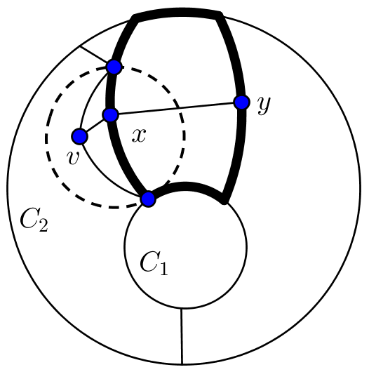
Figure 12: The bold cycle is $C(xy)$ and the dashed cycle is $\Sigma(xy,S_{xy})$.

4 Correctness of spanner

In this section, we prove the correctness of our spanner. Let $\mathrm{OPT}$ be the weight of an optimal solution for 3-ECP. Then the correctness requires two parts: (1) bounding its weight by $O(\mathrm{OPT})$ and (2) showing it contains a $(1+\epsilon)$-approximation of the optimal solution. The weight of our spanner is bounded by the weight of mortar graph, which we briefly introduce in Subsection 4.1.

The following Structure Theorem guarantees that there is a nearly-optimal solution in our spanner and completes the correctness of our spanner:

Theorem 38 (Structure Theorem).

For any $\epsilon>0$ and any planar graph instance $(G,w,r)$ of 3-ECP, there exists a feasible solution $S$ in our spanner such that

• the weight of $S$ is at most $(1+c\epsilon)\mathrm{OPT}$ where $c$ is an absolute constant, and

• the intersection of $S$ with the interior of any brick is a set of trees whose leaves are on the boundary of the brick and each tree has a number of leaves depending only on $\epsilon$.

We prove the Structure Theorem in Subsection 4.2. The idea is similar to that for 2-ECP, that is we transform an optimal solution to a feasible solution satisfying the theorem. Throughout we indicate where the transformation for 3-ECP departs from those of 2-ECP. In the following, we denote by $Q$ the set of terminals, which are the vertices with positive requirement.

4.1 Mortar graph, bricks and portals

The Mortar graph is a grid-like subgraph of $G$ that (1) spans $Q$ and (2) has weight at most $9\epsilon^{-1}$ times the weight of a minimum Steiner tree that spans $Q$. Since the weight of minimum Steiner tree is no more than OPT, the weight of mortar graph is no more than $9\epsilon^{-1}\mathrm{OPT}$. A brick $B$ is the subgraph of $G$ that is enclosed by a face of the mortar graph (including the boundary of the face); it has boundary $\partial B$ and interior $\mathrm{int}(B)=G[E(B)\setminus E(\partial B)]$. Further, bricks have the following property:

Lemma 39.

(Lemma 6.10 [10]) The boundary of a brick $B$, in counterclockwise order, is the concatenation of four paths $W_{B}$, $S_{B}$, $E_{B}$ and $N_{B}$ (west, south, east and north) such that:

1. The set of edges $B\setminus\partial B$ is nonempty.

2. Every vertex of $Q\cap B$ is in $N_{B}$ and $S_{B}$.

3. $N_{B}$ is 0-short and every proper subpath of $S_{B}$ is $\epsilon$-short.

4. There exists a number $t\leq\kappa(\epsilon)$ and vertices $s_{0},s_{1},\dots,s_{t}$ ordered from west to east along $S_{B}$ such that for any vertex $x$ of $S_{B}[s_{i},s_{i+1})$, the distance from $x$ to $s_{i}$ along $S_{B}$ is less than $\epsilon$ times the distance from $x$ to $N_{B}$ in $B$.

For the above lemma, a path is $\epsilon$-short if the distance between every pair of vertices on that path is at most $(1+\epsilon)$ times the distance between them in $G$ and $\kappa(\epsilon)=4\epsilon^{-2}(1+\epsilon^{-1})$. The paths that forms eastern and western boundaries of bricks are called supercolumns, and further satisfy:

Lemma 40.

(Lemma 6.6 [10]) The sum of the weight of all edges in supercolumns is at most $\epsilon\mathrm{OPT}$.

To obtain the spanner, we add a set of Steiner trees in each brick $B$ whose terminals are vertices of $\partial B$. The terminals are drawn from a subset of portal vertices evenly spaced on the boundary of each brick. We bound the number of portals per brick by $\theta(\epsilon)=O(\epsilon^{-2}\alpha(\epsilon))$ and $\alpha(\epsilon)$ in turn depends on the number of connections required to allow a nearly optimal solution, which is bounded by $o(\epsilon^{-5.5})$. The portals satisfy:

Lemma 41.

(Lemma 7.1 [10]) For any vertex $x$ on $\partial B$, there is a portal $y$ such that the weight of $x$-to-$y$ subpath of $\partial B$ is at most $1/\theta(\epsilon)$ times the weight of $\partial B$.

Since the weight of each Steiner tree in a brick $B$ can be bounded by the weight of the weight of $\partial B$, and since there are only constant number (that is $2^{\theta(\epsilon)}$) of such Steiner trees, the weight of all trees we add in $B$ is at most $f(\epsilon)$ times the weight of $\partial B$. So the total weight of our spanner is bounded by $(2f(\epsilon)+9\epsilon^{-1})$ times the weight of $MG$, which is $O(\mathrm{OPT})$.

4.2 Proof of the Structure Theorem

We transform $\mathrm{OPT}$ for the instance $(G,Q,r)$ so that it satisfies the following properties (repeated from the introduction):

P1:

$\mathrm{OPT}\cap\mathrm{int}(B)$ can be partitioned into a set of trees $\mathcal{T}$ whose leaves are on the boundary of $B$.

P2:

If we replace any tree in $\mathcal{T}$ with another tree spanning the same leaves, the result is a feasible solution.

P3:

There is another set of $O(1)$ trees $\mathcal{T}^{\prime}$ that costs at most a $1+\epsilon$ factor more than $\mathcal{T}$, such that each tree of $\mathcal{T}^{\prime}$ has $O(1)$ leaves and $(\mathrm{OPT}\setminus{\mathcal{T}})\cup{\mathcal{T}}^{\prime}$ is a feasible solution.

To argue about the leaves of trees on the boundary of bricks, we use the following definition:

Definition 1.

(Joining vertex [9]). Let $H$ be a subgraph of $G$ and $P$ be a subpath of $\partial G$. A joining vertex of $H$ with $P$ is a vertex of $P$ that is the endpoint of an edge of $H-P$.

The transformation consists of the following steps:

Augment

We add four copies of each supercolumn; we take two copies each to be interior to the two adjacent bricks. After this, connectivity between the east and west boundaries of a brick will be transformed to that between the north and south boundaries. By Lemma 40, this only increases the weight by an small fraction of $\mathrm{OPT}$.

Cleave

By cleaving a vertex, we split it into multiple copies while keeping the connectivity as required by adding artificial edges of weight zero between two copies and maintaining a planar embedding. We call the resulting solution $\mathrm{OPT}_{C}$. In this step, we turn $k$-edge-connectivity into $k$-vertex-connectivity for $k=1,2,3$. By Theorem 18, we can obtain Property P1: $\mathrm{OPT}_{C}\cap\mathrm{int}(B)$ can be partitioned into a set $\cal T$ of trees whose leaves are in $\partial B$. By Corollary 5, we can obtain Property P2: we can obtain another feasible solution by replacing any tree in $\cal T$ with another tree spanning the same leaves.

Flatten

For each brick $B$, we consider the connected components of $\mathrm{OPT}_{C}\cap\mathrm{int}(B)$. If the component only spans vertices in the north or south boundary, we replace it with the minimum subpath of the boundary that spans the same vertices. This will not increase the weight much by the $\epsilon$-shortness of the north and south boundaries. Note that vertex-connectivity may bread as a result, but edge-connectivity is maintained. In the remainder, we only maintain edge-connectivity. We call the resulting solution $\mathrm{OPT}_{F}$.

Restructure

For each brick $B$, we consider the connected components of $\mathrm{OPT}_{F}\cap\mathrm{int}(B)$. We replace each component with a subgraph through a mapping $\phi$. The new subgraph may be a tree or a subgraph $\widehat{C}$ given by Lemma 43. The mapping $\phi$ has the following properties:

1. For any component $\chi$ of $\mathrm{OPT}_{M}\cap\mathrm{int}(B)$, $\phi(\chi)$ is connected and spans $\chi\cap\partial B$.

2. For two components $\chi_{1}$ and $\chi_{2}$ of $\mathrm{OPT}_{M}\cap\mathrm{int}(B)$, if $\phi(\chi_{i})\neq\widehat{C}$ for at least one of $i=1,2$, then $\phi(\chi_{1})$ and $\phi(\chi_{2})$ are edge-disjoint, taking into account edge multiplicities.

3. The new subgraph $\phi($OPT${}_{M}\cap\mathrm{int}(B))$ has $\alpha(\epsilon)=o(\epsilon^{-5.5})$ joining vertices with $\partial B$.

We can prove that the total weight is increased by at most $\epsilon\mathrm{OPT}_{F}$, giving Property P3. We call the resulting solution $\mathrm{OPT}_{R}$.

Redirect

We connect each joining vertex $j$ of $\mathrm{OPT}_{R}\cap\mathrm{int}(B)$ to the nearest portal $p$ on $\partial B$ by adding multiple copies of the short $j$-to-$p$ subpath of $\partial B$. We call the resulting solution $\widehat{OPT}$.

We give more details of these transformations in the following subsections and argue that the transformations guarantee the required connectivity as we do so. These details are very similar to that used for 2-ECP; we note the differences. The Restructure step which requires a different structural lemma than used for Borradaile and Klein’s PTAS for 2-ECP [8]; the difference between Lemma 43 and that used by Borradaile and Klein is that $\widehat{C}$ need only be a cycle for the 2-ECP, whereas to maintain 3-edge connectivity, a more complicated subgraph $\widehat{C}$ is required. We borrow the following lemma from [8] to prove Lemma 43.

Lemma 42.

(Simplifying a tree with one root, Lemma 10.4 [10]). Let $r$ be a vertex of $T$. There is another tree $\widehat{T}$ that spans $r$ and the vertices of $T\bigcap P$ such that $w(\widehat{T})\leq(1+4\epsilon)w(T)$ and $\widehat{T}$ has at most $11\epsilon^{-1.45}$ joining vertices with $P$.

Lemma 43.

Let $\mathcal{F}$ be a set of non-crossing trees whose leaves are joining vertices with $\epsilon$-short paths $P_{1}$ and $P_{2}$ on the boundary of the graph, and each tree in $\mathcal{F}$ has leaves on both paths. Then there is a subgraph or empty set $\widehat{C}$, a set $\widehat{\mathcal{F}}$ of trees, and a mapping $\phi:\mathcal{F}\to\widehat{\mathcal{F}}\cup\widehat{C}$ with the following properties

• For every tree $T$ in $\mathcal{F}$, $\phi(T)$ spans $T$’s leaves.

• For two trees $T_{1}$ and $T_{2}$ in $\mathcal{F}$, if $\phi(T_{i})\neq\widehat{C}$ for at least one of $i=1,2$ then $\phi(T_{1})$ and $\phi(T_{2})$ are edge-disjoint (taking into account edge multiplicities).

• The subgraph $\bigcup\widehat{\mathcal{F}}\cup\{\widehat{C}\}$ has $o(\epsilon^{-2.5})$ joining vertices with $P_{1}\cup P_{2}$.

• $w(\widehat{C})+w(\widehat{\mathcal{F}})\leq 6w(P_{2})+(1+d\cdot\epsilon)w(\mathcal{F})$, where $d$ is an absolute constant.

• Any two vertices of $\widehat{C}\cap(P_{1}\cup P_{2})$ are three-edge-connected.

• For any three pairs of vertices of $\widehat{C}\cap(P_{1}\cup P_{2})$ (where vertices may be repeated), $\widehat{C}$ contains three edge-disjoint paths connecting them respectively.

Proof.

Call $P_{1}$ the top path and $P_{2}$ the bottom path. Order the trees of $\mathcal{F}$: $T_{1},T_{2},\ldots,T_{k}$ according to their leaves on $P_{2}$ from left-to-right; the trees are well ordered since they are non-crossing and have leaves on both paths. There are two cases:

$k>\epsilon^{-1}$:

In this case we reduce the number of trees by incorporating a subgraph $\widehat{C}$. Let $a$ be the smallest index such that $w(T_{a})\leq\epsilon w(\mathcal{F})$ and $b$ the largest index such that $w(T_{b})\leq\epsilon w(\mathcal{F})$. We replace trees $T_{a},T_{a+1},\dots,T_{b}$ with a subgraph $\widehat{C}$. Let $P^{\prime}_{1}$ be the minimal subpath of $P_{1}$ that spans all the leaves of tree $T_{i}$ for $a\leq i\leq b$. $P^{\prime}_{2}$ is likewise the minimal subpath on $P_{2}$. Let $u_{i}$ and $v_{i}$ be $P^{\prime}_{i}$’s endpoints (with $u_{i}$ the left end) for $i=1,2$. Let $P_{a}$ ($P_{b}$) be the $u_{1}$-to-$u_{2}$ ($v_{1}$-to-$v_{2}$) subpath in $T_{a}$ ($T_{b}$). Since $P_{1}$ is $\epsilon$-short, we have

$$w(P^{\prime}_{1})\leq(1+\epsilon)w(P_{a}\cup P_{b}\cup P^{\prime}_{2}).$$

Let $\widehat{C}$ be the multisubgraph $\{P_{a},P_{a},P_{b},P^{\prime}_{1},P^{\prime}_{1},P^{\prime}_{2},P^{\prime}_{2}\}$. We replace $\bigcup_{i=a}^{b}T_{i}$ with $\widehat{C}$ and set $\phi(T_{i})=\widehat{C}$ for $a\leq i\leq b$.

$k\leq\epsilon^{-1}$:

In this case, the number of trees is already bounded and we set $\widehat{C}=\emptyset$.

In both cases, we transform the remaining trees $T_{i}$ ($i\neq a,a+1,\dots,b$) as follows. Let $T^{\prime}_{i}$ be a minimal subtree of $T_{i}$ that spans all leaves of $T_{i}$ on $P_{1}$ and exactly one vertex $r$ on $P_{2}$. Let $R_{i}$ be the minimal subpath on $P_{2}$ that spans all leaves of $T_{i}$ on $P_{2}$. By Lemma 42, there is another tree, say $T^{\prime\prime}_{i}$, for $T^{\prime}_{i}$ with root $r$ and path $P_{1}$. We replace $T_{i}$ with $\widehat{T_{i}}=T^{\prime\prime}_{i}\cup R_{i}$, and set $\phi(T_{i})=\widehat{T_{i}}$ for $i\neq a,\dots,b$. Then $\widehat{T_{i}}$ spans all leaves of $T_{i}$.

$\widehat{C}$ (if non-empty) has six joining vertices with $P_{1}\cup P_{2}$. Each tree $\widehat{T_{i}}$ has one joining vertex with $P_{2}$ and by Lemma 42 $o(\epsilon^{-1.5})$ joining vertices with $P_{1}$. By the choice of $a$ and $b$, there are at most $\epsilon^{-1}$ trees mapped to $\widehat{T_{i}}$. So $\widehat{\mathcal{F}}\cup\{\widehat{C}\}$ has totally at most $o(\epsilon^{-2.5})$ joining vertices with $P_{1}\cup P_{2}$.

The total weight of $\widehat{C}$ is

$$\begin{array}[]{llll}w(\widehat{C})&\leq 2w(P^{\prime}_{1})+2w(P^{\prime}_{2})+2w(P_{a})+w(P_{b})\\ &\leq 2(1+\epsilon)[w(P_{a})+w(P_{b})+w(P^{\prime}_{2})]+2w(P^{\prime}_{2})+2w(P_{a})+w(P_{b})\\ &\leq(4+2\epsilon)w(P_{a})+(3+2\epsilon)w(P_{b})+(4+2\epsilon)w(P^{\prime}_{2})\\ &\leq(7+4\epsilon)\epsilon\cdot w(\mathcal{F})+(4+2\epsilon)w(P^{\prime}_{2}).\\ \end{array}$$

And the total weight of $\widehat{T_{i}}$ is

$$\begin{array}[]{llll}\sum_{i=1,\dots,a-1,b+1,\dots,k}w(\widehat{T_{i}})&\leq\sum_{i=1,\dots,a-1,b+1,\dots,k}(w(R_{i})+(1+4\epsilon)w(T_{i})).\end{array}$$

Since all the trees in $\mathcal{F}$ are non-crossing, $R_{i}$ and $P^{\prime}_{2}$ are disjoint. The total weight of our replacement is at most $6w(P_{2})+(1+O(\epsilon))w(\mathcal{F})$.

Now we prove the connectivity properties for $\widehat{C}$. By its construction, $\widehat{C}$ spans all the leaves of tree $T_{i}$ for $a\leq i\leq b$ and vertices of $\widehat{C}\cap(P_{1}\cup P_{2})$ are three-edge-connected. So we only need to prove $\widehat{C}$ contains three edge-disjoint paths connecting any three pair of vertices of $\widehat{C}\cap(P_{1}\cup P_{2})$ respectively. This can be seen by case analysis, as described and illustrated below. Let $P^{*}=P_{a}\cup P^{\prime}_{1}\cup P^{\prime}_{2}$, then every edge of $P^{*}$ has multiplicity of two in $\widehat{C}$ by construction.

We first consider the case that any two pairs do not contain identical vertex. For $i=1,2$ let $x_{i}$, $y_{i}$ and $z_{i}$ be the three pair of vertices. If there are two pairs of vertices are not interleaving in $P^{*}$, then we could connect these two pairs by $P^{*}\cup P_{b}$, which is a cycle. And the other pair could be connected by a subpath of $P^{*}$ which is edge-disjoint from the other two paths in $\widehat{C}$. Otherwise, we have the two sets, $\{x_{i},y_{j},z_{l}\}$ and $\{x_{3-i},y_{3-j},z_{3-l}\}$, which do not interleave each other and appear in the same order in $P^{*}$. See Figure 13: there are three edge-disjoint paths connecting the three pairs respectively.

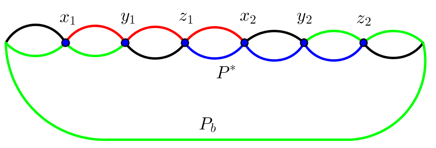
Figure 13: If every two pairs of the three interleave, there are three edge-disjoint paths, shown in different colors, connecting them respectively in $\widehat{C}$.

If there are two pairs containing identical vertices, we could connect these two pairs by $P^{*}\cup P_{b}$ and then connect the other pair by another subpath of $P^{*}$. Since every edge in $P^{*}$ is multiple in $\widehat{C}$, these paths are edge-disjoint. ∎

4.2.1 Augment

For each supercolumn $P$ common to two bricks $B_{1}$ and $B_{2}$, we do the following:

• Add four copies of $P$, $P_{1},P_{2},P_{3},P_{4}$ to $\mathrm{OPT}$. We consider $P_{1}$ and $P_{2}$ to be internal to $B_{1}$, and $P_{3}$ and $P_{4}$ to be internal to $B_{2}$. We also cut open the graph along $P$, creating a new face between $P_{2}$ and $P_{3}$. Call the result $\mathrm{OPT}^{\prime}_{A}$.

• Remove edges from $\mathrm{OPT}^{\prime}_{A}$ until what remains a minimal subgraph satisfying the connectivity requirements. Similar to the argument illustrated in Figure 13, maintaining connectivity in the presence of this new face is achievable.

Let the resulting solution be $\mathrm{OPT}_{A}$. By this construction, $\mathrm{OPT}_{A}$ has no joining vertices with internal vertices of the supercolumns:

Lemma 44.

For every brick $B$, the joining vertices of OPT${}_{A}\cap B$ with $\partial B$ belong to $N_{B}$ and $S_{B}$.

4.2.2 Cleave

In this part, we call the vertices with positive requirement terminals. Given a vertex $v$ with a non-interleaving bipartition $A$ and $B$ of the edges incident to $v$, we define cleaving $v$ as the following: split $v$ into two copies $v_{1}$ and $v_{2}$, such that all the edges in $A$ ($B$) are incident to $v_{1}$ ($v_{2}$); and then we add one zero-weight edge between $v_{1}$ and $v_{2}$. See Figure 14. We have two types of cleavings:

Simplifying cleavings Let $C$ be a non-self-crossing, non-simple cycle that visits vertex $v$ twice. For $1\leq i\leq 4$, let $e_{i}$ be the edge of $C$ incident to $v$ such that $e_{1}$, $e_{2}$, $e_{3}$ and $e_{4}$ are embedded clockwise and $e_{1}$ and $e_{4}$ are in the same subcycle of $C$. Define a bipartition $A$, $B$ of the edges incident to $v$ as follows: given the clockwise embedding of those edges, let $A$ contain $e_{1}$, $e_{2}$ and all the edges between them clockwise.

Lengthening cleavings Let $C$ be a cycle and $v$ a vertex on $C$. Let $e_{1}$ and $e_{2}$ be the edges incident to $v$ strictly inside of $C$, and let $e^{\prime}_{1}$ and $e^{\prime}_{2}$ be the edges of $C$ incident to $v$. Define a bipartition $A$ and $B$ of the edges incident to $v$ as follows: given the embedding of those edges with $e_{1}$, $e_{2}$, $e^{\prime}_{2}$ and $e^{\prime}_{1}$ in the clockwise order, $A$ contains $e_{1}$, $e^{\prime}_{1}$ and all the edges from $e^{\prime}_{1}$ to $e_{1}$ clockwise.

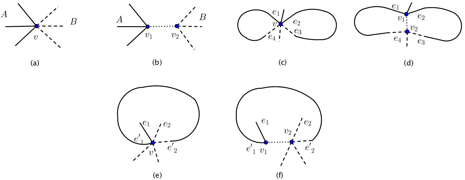
Figure 14: Cleaving examples. The bipartition of edges incident to $v$ is illustrated by solid edges $A$ and dashed edges $B$, and the added artificial edge is illustrated by the dotted edge. (a) and (b) give an example before and after a cleaving. (c) and (d) illustrate a simplifying cleaving. (e) and (f) show a lengthening cleaving.

We perform simplifying cleavings for all the non-simple cycles of OPT_A until every cycle is simple and call the resulting solution OPT${}^{\prime}_{S}$ and the resulting graph $G_{S}$. Note that after simplifying cleaving a terminal, we take only one copy that is in the mortar graph as the terminal. These cleavings will reduce edge-connectivity to vertex-connectivity by the following lemmas.

Lemma 45.

For the cleaved vertex $v$, the copies of $v$ are three-edge-connected in OPT${}^{\prime}_{S}$.

Proof.

The original cycle will give two edge-disjoint paths between the two copies. And the artificial edge will be the third path. ∎

Lemma 46.

Let $\widehat{H}$ be the graph obtained from $H$ by a simplifying cleaving a vertex $v$. Then for $k=1,2,3$, if a vertex $u$ and $v$ are $k$-edge-connected in $H$, then $u$ and any copy of $v$ are $k$-edge-connected in $\widehat{H}$.

Proof.

If $u$ and $v$ are $k$-edge-connected, then there are $k$ edge-disjoint paths from $u$ to $\{v_{1},v_{2}\}$. Since $k$ is no more than three, and $v_{1}$ and $v_{2}$ are three-edge-connected by Lemma 45, $u$ and $v_{1}$ are $k$-edge-connected. Similarly, $u$ and $v_{2}$ are $k$-edge-connected. ∎

Corollary 47.

For $k=1,2,3$, if two vertices are $k$-edge-connected in OPT_A, then any of their copies are $k$-edge-connected in OPT${}^{\prime}_{S}$.

We then remove edges from OPT${}^{\prime}_{S}$ until the rest is a minimal subgraph satisfying the connectivity requirement. We call the resulting solution OPT_S. Since every cycle in OPT_S is simple, we have the following lemma:

Lemma 48.

For $k=1,2,3$, if two terminals are $k$-edge-connected in OPT_A, then they are $k$-vertex-connected OPT_S.

Let $Q_{23}$ be set of terminals whose requirement is at least two and $H$ be the minimal $(Q_{23},r)$-vertex-connected subgraph in $\mathrm{OPT}_{S}$. Since every cycle in OPT_S is simple, we know that $H$ also has this property. It follows that the degree of any vertex $v$ of $H$ is no more than three, since $H$ is biconnected by Lemma 7: for otherwise, let the first ear (a cycle) contain $v$ and let the second and third ear start with the next two edges incident to $v$ – from these ears it is easy to construct two cycles that only meet at $v$, witnessing a non-simple cycle.

We perform lengthening cleavings w.r.t. the boundary of each brick and the edges of $\mathrm{OPT}_{S}$ that are incident to a boundary vertex in that brick until the vertices of the brick boundaries have at most one edge in the solution in the interior of each incident brick. We add the introduced zero-length edges to the solution. Call the new solution $\mathrm{OPT}_{C}$ and the new graph and mortar graph $G_{C}$ and $MG_{C}$, respectively.

For each cleaved terminal, we assign only one copy to be the terminal: we pick the copy of highest degree in $\mathrm{OPT}_{C}$ to be the terminal; note that terminals are still in the mortar graph. Although the flatten, restructure and redirect steps may break the vertex connectivity guaranteed by Lemma 45, the following lemmas will guarantee that edge-connectivity will not be preserved.

Lemma 49.

For $k=1,2,3$, if terminals are $k$-vertex-connected in $\mathrm{OPT}_{S}$, then they are $k$-vertex-connected $\mathrm{OPT}_{C}$. Further, $\mathrm{OPT}_{C}$ is minimal.

Proof.

Borradaile and Klein prove (Lemma 5.9 [9]) that lengthening cleavings maintain biconnectivity, so we need only argue that terminals $a$ and $b$ that are triconnected in $\mathrm{OPT}_{S}$ have terminal copies $a^{\prime}$ and $b^{\prime}$ that are triconnected in $\mathrm{OPT}_{C}$.

Consider three, vertex-disjoint $a$-to-$b$ paths $P_{1},P_{2},P_{3}$ in $\mathrm{OPT}_{S}$. As argued earlier, the degrees of $a$ and $b$ in $\mathrm{OPT}_{S}$ are three. The terminal copy $a^{\prime}$ of $a$ likewise has degree 3 in $\mathrm{OPT}_{C}$: if $a$ is lengthening cleaved, then there is a copy of $a$ that has degree 3.

The paths $P_{1},P_{2},P_{3}$ map to paths $P_{1}^{\prime},P_{2}^{\prime},P_{3}^{\prime}$ between copies of $a$ and $b$ in $\mathrm{OPT}_{C}$: if an internal vertex of $P_{i}$ is lengthening cleaved, then include the introduced edge in the path. The endpoints of $P_{i}^{\prime}$ that map to copies of, w.l.o.g., $a$ are likewise connected by introduced edges (if $a$ is subject to a lengthening cleaving). Let $a^{\prime}$ be the terminal copy of $a$; we augment the paths $P_{i}^{\prime}$ to connect to $a^{\prime}$ via an introduced, zero-weight edge. Doing so for $b^{\prime}$ as well gives three vertex disjoint $a^{\prime}$-to-$b^{\prime}$ paths in $\mathrm{OPT}_{C}$.

That $\mathrm{OPT}_{C}$ is minimal follows directly from the fact that $\mathrm{OPT}_{S}$ is minimal. ∎

The following lemma was proved by Borradaile and Klein for 2-ECP (Lemma 5.10 [9]); their proof only relied on the fact that every cycle contains a terminal. Since this is true for the 3-ECP too (Theorem 18), we get the same lemma:

Lemma 50.

Let $B$ be a brick in $G_{C}$ with respect to $MG_{C}$. The intersection OPT${}_{C}\cap\mathrm{int}(B)$ is a forest whose joining vertices with $\partial B$ are all the leaves of the forest.

Lemma 51.

Let $x$ and $y$ be two terminals in OPT_C such that $k=\min\{r(x),r(y)\}\geq 2$ and let $B$ be a brick. There exist $k$ vertex-disjoint paths from $x$ to $y$ such that for any two such paths $P_{1}$ and $P_{2}$, any connected component of $P_{1}\cap\mathrm{int}(B)$ and any connected component of $P_{2}\cap\mathrm{int}(B)$ belong to distinct components of OPT${}_{C}\cap\mathrm{int}(B)$.

Proof.

Let $H_{C}$ be the minimal $(Q_{23},r)$-vertex-connected subgraph in OPT_C. Then each connected component of OPT${}_{C}\setminus H_{C}$ is a tree and is connected to $H_{C}$ by one edge. By Corollary 5, there are $min\{r(x),r(y)\}$ vertex-disjoint paths from $x$ to $y$ in $H_{C}$ (and then in OPT_C) such that any path connecting any two of those $x$-to-$y$ paths contains a terminal. Let $P_{1}$ and $P_{2}$ be any two such $x$-to-$y$ paths. Since all terminals are on the boundaries of bricks, any $P_{1}$-to-$P_{2}$ path in $\mathrm{int}(B)$ will be divided into two subpaths by some lengthening cleaving. So any connected component of OPT${}_{C}\cap\mathrm{int}(B)$ can not contain the components of both $P_{1}\cap\mathrm{int}(B)$ and $P_{2}\cap\mathrm{int}(B)$. ∎

4.2.3 Flatten

This step is the same as described by Borradaile and Klein for 2-ECP [9]. For each brick $B$, consider the edges of OPT${}_{C}\cap\mathrm{int}(B)$. By Lemma 50, the connected components of OPT${}_{C}\cap\mathrm{int}(B)$ are trees. By Lemma 44, every leaf is either on $N_{B}$ or $S_{B}$. For every tree whose leaves are all on $N_{B}$ ($S_{B}$), we replace the tree with the minimal subpath of $N_{B}$ ($S_{B}$) that contains all its leaves. Let the resulting solution be OPT_F. By Lemma 51, this guarantees 2- and 3-edge-connectivity between terminals as required; trees may be flattened against a common $\epsilon$-short path that is the northern boundary of one brick and the southern boundary of another, so vertex-connectivity gets broken at this stage.

4.2.4 Restructure

This step is the same as described by Borradaile and Klein for 2-ECP [9], except we apply our 3-ECP specific lemma (Lemma 43). Restructuring replaces $\mathrm{OPT}_{F}\cap\mathrm{int}(B)$, which is a set of non-crossing trees (Lemma 50) with leaves on the $\epsilon$-short north and south brick boundaries (Lemma 44), with subgraphs guaranteed by Lemma 43. The resulting solution is $\mathrm{OPT}_{R}$.

Let ${\cal P}_{xy}$ be a set of 2 (3) vertex disjoint paths in $\mathrm{OPT}_{F}$ for terminals $x,y$ requiring bi- (tri-)connectivity. Each path in ${\cal P}_{xy}$ is broken into a sequence of small paths, each of which is either entirely in the interior of a brick or entirely in the mortar graph. Let ${\cal P}_{xy}^{\prime}$ be the set of these path sequences.

We define a map $\hat{\phi}$ for the paths in ${\cal P}_{xy}^{\prime}$. For a path $P$ of $\mathcal{P}^{\prime}_{xy}$, if $P$ is on mortar graph, we define $\hat{\phi}(P)=P$; otherwise we define $\hat{\phi}(P)=\phi(T)$ where $T$ is the tree in OPT_M containing $P$. Since $\phi(T)$ spans all leaves of $T$, $\hat{\phi}(P)$ also spans leaves of $T$ and connects endpoints of $P$.

Let $P_{1}$ and $P_{2}$ be any two paths from distinct path-sequences inside of the same brick $B$. By Lemma 51, $P_{1}$ and $P_{2}$ can not belong to the same component of OPT${}_{M}\cap\mathrm{int}(B)$. So if $\hat{\phi}(P_{1})\neq\hat{\phi}(P_{2})$, then $\hat{\phi}(P_{1})$ and $\hat{\phi}(P_{2})$ are edge disjoint by the constructions of $\phi$ and $\hat{\phi}$. Otherwise, we know the image is a subgraph $\widehat{C}$ which guarantees triconnectivity for all vertices of $\widehat{C}\cap\partial B$ by Lemma 43. However, there may be more than one paths from any path-sequence whose image is $\widehat{C}$, and the new $x$-to-$y$ paths may not be edge-disjoint in $\widehat{C}$. For this situation, we could shortcut the paths in $\widehat{C}$ such that each new $x$-to-$y$ path only contain one subpath in $\widehat{C}$. Since there are at most three such subpaths and there endpoints are in $\partial B$, $\widehat{C}$ contains edge-disjoint paths connecting the endpoints of those subpaths by the last property of Lemma 43.

Therefore, the restructure step maintains that if terminals were 1-, 2- or 3-edge connected in $\mathrm{OPT}_{F}$, then they still are in $\mathrm{OPT}_{R}$. We also see that, by construction of Lemma 43, the intersection $\mathrm{OPT}_{R}$ with the interior of a brick $B$ is a set of trees with leaves on $\partial B$. Since the Redirect step will only add edges of $\partial B$, this property does not change, proving one of the guarantees of the Structure Theorem.

Further, the number of joining vertices is guaranteed by Lemma 43 and the construction that is used for 2-ECP. The number of joining vertices is on the same order as for 2-ECP, which depends only on $\epsilon$ as required.

4.2.5 Redirect

For every joining vertex $j$ of $\mathrm{OPT}_{R}\cap B$ with $\partial B$ for a brick $B$, we add the path from $j$ to the nearest portal $p$ on $\partial B$. This guarantees that the trees guaranteed by the Restructure step have leaves that are portals: this allows us to efficiently enumerate all possible Steiner trees in bricks whose terminals are portals to compute the spanner graph.

4.2.6 Analysis of weight increase

The analysis of the weight increase is exactly the same as for 2-ECP by Borradaile and Klein; the only difference are the weight in Lemma 43 which is on the order of the weight in the equivalent Lemma used in 2-ECP.

This completes the proof of the Structure Theorem.

5 Dynamic programming for $k$-ECP on graphs with bounded branchwidth

In this section, we give a dynamic program to compute the optimal solution of $k$-ECP problem on graphs with bounded branchwidth. This is inspired by the work of Czumaj and Lingas [11, 12]. Note that such graphs need not be planar. This can be used in our PTAS after the contraction step of the framework.

A branch decomposition of a graph $G=(V(G),E(G))$ is a hierarchical clustering of $E(G)$. It can be represented by a binary tree, called the decomposition tree, the leaves of which are in bijection with the edges of $G$. After deleting an edge $e$ of this decomposition tree, $E(G)$ is partitioned into two parts $E_{1}$ and $E_{2}$ according to the edges mapped to the leaves of the two subtrees. All the vertices common to $E_{1}$ and $E_{2}$ comprise the separator corresponding to $e$ in the decomposition. The width of the decomposition is the maximum size of the separator in that decomposition. The branchwidth of $G$ is the minimum width of any branch decomposition of $G$.

Let $G=(V(G),E(G),r)$ be an instance of $k$-ECP. Then $r\in\{0,1,\cdots,k\}$. We call a vertex a terminal if its requirement is positive. We first augment $G$ such that each edge becomes $k$ parallel edges. Our dynamic programming will work on this new graph $G$. Given a branch decomposition of $G$, root the decomposition tree $T$ at an arbitrary leaf. For any node $q$ in $T$, let $L$ be the separator corresponding to its parent edge, and $E_{1}$ be the subset of $E(G)$ mapped to the leaves in the subtree rooted at $q$. Let $H$ be a subgraph of $G[E_{1}]$ such that it contains all terminals in $G[E_{1}]$. An separator completion of $L$ is a multiset of edges between vertices of $L$, each of which may appear up to $k$ times. A configuration of a terminal $v$ of $H$ in $L$ is a tuple $(A,B,r(v))$, where $A$ is a tuple $(a_{1},a_{2},\dots,a_{|L|})$, representing that there are $a_{i}$ edge-disjoint paths from $v$ to the $i$th vertex of $L$ in $H$, and $B$ is a set of tuples $(x_{i},y_{i},b_{i})$, representing that there are $b_{i}$ edge-disjoint paths between the vertices $x_{i}$ and $y_{i}$ of $L$ in $H$. All the $\sum_{i=1}^{|L|}a_{i}+\sum_{i}b_{i}$ paths in a configuration are mutually edge-disjoint in $H$. We adapt a definition of Czumaj and Lingas [11, 12]:

Definition 2.

For any pair of terminals $u$ and $v$ in $H$, let $Com_{H}(u,v)$ be the set of separator completions of $H$ each of which augments $H$ to a graph where $u$ and $v$ satisfy the edge-connectivity requirement. For each terminal $v$ in $H$, let $Path_{H}(v)$ be a set of configurations of $v$ on $L$. Let $Path_{H}$ be the set of all the non-empty $B$ in which all tuples can be satisfied in $H$. Let $C_{H}$ be the set consisting of one value in each $Com_{H}(u,v)$ for all pairs of terminals $u$ and $v$ in $H$, and $P_{H}$ be the set consisting of one value in each $Path_{H}(v)$ for all terminal $v$ in $H$. We call the tuple $(C_{H},P_{H},Path_{H})$ the connectivity characteristic of $H$, and denote it by $Char(H)$.

Let $w$ be the width of the decomposition. Then $|L|\leq w$. Note that $H$ may correspond to multiple $C_{H}$ and $P_{H}$, so $H$ may have multiple connectivity characteristics. Further, each value in $P_{H}$ represents at least one terminal. For any $L$, there are at most $k^{O(w^{2})}$ distinct separator completions ($O(w^{2})$ pairs of vertices, each of which can be connected by at most $k$ parallel edges) and at most $2^{k^{O(w^{2})}}$ distinct sets $C_{H}$ of separator completions. For any $L$, there are at most $k^{O(w^{2})}$ different configurations for any terminal in $H$ since the number of different sets $A$ is at most $k^{w}$, the number of different sets $B$ is at most $k^{O(w^{2})}$ (the same as the number of separator completions) and $k$ different choices for $r(v)$. So there are at most $2^{k^{O(w^{2})}}$ different sets of configurations $P_{H}$, and at most $2^{k^{O(w^{2})}}$ different sets $B$. Therefore, there are at most $2^{k^{O(w^{2})}}$ distinct connectivity characteristics for a fixed $L$.

Definition 3.

A configuration of $v$ on $L$ is connecting if for any terminal $u$ in $V(G)\setminus V(H)$ the inequality $\sum_{i=1}^{|L|}a_{i}\geq\min\{r(v),r(u)\}$ holds where $a_{i}$ is the $i$th coordinate in $A$. That is, there are enough edge-disjoint paths from $v$ to the separator which can connect $u$ and $v$. $Char(H)$ is connecting if all configurations in its $P_{H}$ set are connecting. $H$ is connecting if at least one of $Char(H)$ is connecting. In the following, we only consider connecting connectivity characteristics and subgraphs.

In the following, we need as a subroutine an algorithm to solve the following problem: when given a set of demands $(x_{i},y_{i},b_{i})$ and a multigraph, we want to decide if there exist $b_{i}$ edge-disjoint paths between vertices $x_{i}$ and $y_{i}$ in the graph and all the $\sum_{i}b_{i}$ paths are mutually edge-disjoint. Although we do not have a polynomial time algorithm for this problem, we only need to solve this on graphs with $O(w)$ vertices, $O(kw^{2})$ edges and $O(w^{2})$ demands. So even an exponential time algorithm is acceptable for our purpose here. Let $ALG$ be an algorithm for this problem, whose running time is bounded by a function $f(k,w)$, which may be exponential in both $k$ and $w$.

For a node $p$ of degree three in the decomposition tree $T$, let $q_{1}$ and $q_{2}$ be its two children and $q$ be its parent. Let $T_{i}$ be the subtree of $T$ rooted at $q_{i}$, let $E_{i}$ be the subset of $E(G)$ corresponding to $T_{i}$ and let $L_{i}$ be the separator corresponding to the edge $pq_{i}$ for $i=1,2$. Let $L$ be the separator corresponding to $pq$. For $i=1,2$, let $H_{i}$ be a subgraph of $G[E_{i}]$ that contains all the terminals. Let $H=H_{1}\cup H_{2}$. Then we have the following lemma.

Lemma 52.

For any pair of $Char(H_{1})$ and $Char(H_{2})$, all the possible $Char(H)$ that could be obtained from $Char(H_{1})$ and $Char(H_{2})$ can be computed in $O(k^{w^{2}}f(k,w)+k^{w^{2}k^{w^{2}}})$ time.

Proof.

We compute all the possible sets for the three components of $Char(H)$.

Compute all possible $\mathbf{C_{H}}$ $C_{H}$ contains two parts: the first part covers all pairs of terminals in the same $H_{i}$ for $i=1,2$ and the second part covers all pairs of terminals from distinct subgraphs.

For the first part, we generalize each value $C\in C_{H_{i}}$ for $i=1,2$ into a possible set $X_{C}$. Notice that each separator completion can be represented by a set of demands $(x,y,b)$. For a candidate separator completion $C^{\prime}$ on $L$, we combine $C^{\prime}$ with each $B\in Path_{H_{3-i}}$ to construct a graph $H^{\prime}$ and define the demand set the same as $C$. By running $ALG$ on this instance, we can check if $C^{\prime}$ is a legal generalization for $C$. This may be computed in $k^{O(w^{2})}w^{2}+k^{O(w^{2})}f(k,w)$ time for each $C$. All the legal generalizations for $C$ form $X_{C}$.

Now we compute the second part. For any pair of configurations $(A^{1},B^{1},r(u))\in P_{H_{1}}$ and $(A^{2},B^{2},r(v))\in P_{H_{2}}$ for $u\in H_{1}$ and $v\in H_{2}$, we compute possible $Com_{H}(u,v)$. Let $L^{\prime}=L_{1}\cap L_{2}$. We first count how many edge-disjoint paths between $u$ and $v$ could go through $L^{\prime}$ by checking $A^{1}$ and $A^{2}$, and then check if a candidate separator completion $C^{\prime}$ on $L$ can provide the remaining paths. All those $C^{\prime}$ that are capable of providing enough paths form $Com_{H}(u,v)$. This can be computed in $w^{2}k^{O(w^{2})}$ time for each pair of values.

A possible $C_{H}$ consists of each value in $X_{C}$ for every $C\in C_{H_{i}}$ for $i=1,2$ and each value in $Com_{H}(u,v)$ for all pairs of configurations of $P_{H_{1}}$ and $P_{H_{2}}$. To compute all the sets, we need at most $k^{O(w^{2})}w^{2}+k^{O(w^{2})}f(k,w)$ time. There are at most $k^{O(w^{2})}$ sets and each may contain at most $k^{O(w^{2})}$ values. Therefore, to generate all the possible $C_{H}$ from those sets, we need at most $k^{w^{2}k^{O(w^{2})}}$ time.

Compute all possible $\mathbf{P_{H}}$ We generalize each configuration $(A,B,r(v))$ of $v$ in $P_{H_{i}}$ into a possible set $Y_{v}$. For each set $B^{\prime}$ in $Path_{H_{3-i}}$, we construct a graph $H^{\prime}$ by $A$, $B$ and $B^{\prime}$ on vertex set $L_{1}\cup L_{2}\cup\{v\}$: if there are $b$ disjoint paths between a pair of vertices represented in $A$, $B$ or $B^{\prime}$, we add $b$ parallel edges between the same pair of vertices in $H^{\prime}$, taking $O(w^{2})$ time. For a candidate value $(A^{*},B^{*},r(v))$ corresponding to $L$, we define a set of demands according to $A^{*}$ and $B^{*}$ and run $ALG$ on all the possible $H^{\prime}$ we construct for sets in $Path_{H_{3-i}}$. If there exists one such graph that satisfies all the demands, then we add this candidate value into $Y_{v}$. We can therefore compute each set $Y_{v}$ in $k^{O(w^{2})}w^{2}+k^{O(w^{2})}f(k,w)$ time. A possible $P_{H}$ consists of each value in $Y_{v}$. There are at most $k^{O(w^{2})}$ such sets and each may contain at most $k^{O(w^{2})}$ values. So we can generate all possible $P_{H}$ from those sets in $k^{w^{2}k^{O(w^{2})}}$ time.

Compute $\mathbf{Path_{H}}$ For each pair of $B^{1}\in Path_{H_{1}}$ and $B^{2}\in Path_{H_{2}}$, we construct a graph $H^{\prime}$ on vertex set $L_{1}\cup L_{2}$: if two vertices are connected by $b$ disjoint paths, we add $b$ parallel edges between those vertices in $H^{\prime}$. Since each candidate $B^{\prime}$ on $L$ can be represented by a set of demands, we only need to run $ALG$ on all possible $H^{\prime}$ to check if $B^{\prime}$ can be satisfied. We add all satisfied candidates $B^{\prime}$ into $Path_{H}$. This can be computed in $k^{O(w^{2})}w^{2}+k^{O(w^{2})}f(k,w)$ time.

Therefore, the total running time is $O(k^{w^{2}}f(k,w)+k^{w^{2}k^{w^{2}}})$. For each component we enumerate all possible cases, and the correctness follows. ∎

Our dynamic programming is guided by the decomposition tree $T$ from leaves to root. For any node $q$ in $T$, let $T_{q}$ be the subtree of $T$ rooted at $q$ and $L_{q}$ be the separator corresponding $q$’s parent edge. Let $E_{q}$ be the subset of $E(G)$ corresponding to $T_{q}$. For each node $q$, our dynamic programming table is indexed by all the possible connectivity characteristics on the corresponding separator $L_{q}$. Each entry indexed by the connectivity characteristic $Char$ in the table is the weight of the minimum-weight subgraph of $G[E_{q}]$ that contains all the terminals in $G[E_{q}]$ and has $Char$ as its connectivity characteristic.

Base case

For each leaf of $T$, the only subgraph $H$ is the edge $uv$ contained in the leaf and the separator only contains its endpoints $u$ and $v$. There are three cases.

1. Both $u$ and $v$ are not terminals. $Com_{H}(u,v)$ contains all subsets of the multiset of edge $uv$ (up to $k$ times), including the empty set. $P_{H}$ is empty since there is no terminal. $Path_{H}$ contains one set: $\{(u,v,1)\}$.

2. Only one of $u$ and $v$ is a terminal. W.l.o.g. assume $u$ is the terminal. $Com_{H}(u,v)$ contains all subsets of the multiset of edge $uv$ (up to $k$ times), including the empty set. $Path_{H}(u)$ contains two configurations: $((k,0),\{(u,v,1)\},r(u))$ and $((k,1),\emptyset,r(u))$. $Path_{H}$ contains one set: $\{(u,v,1)\}$.

3. Both $u$ and $v$ are terminals. $Com_{H}(u,v)$ contains the multisets of edge $uv$ that appears at least $\min\{r(u),r(v)\}-1$ times. $Path_{H}(u)$ contains two configurations: $((k,0),\{(u,v,1)\},r(u))$ and $((k,1),\emptyset,r(u))$, and $Path_{H}(v)$ contains two configurations: $((0,k),\{(u,v,1)\},r(v))$ and $((1,k),\emptyset,r(v))$. $Path_{H}$ contains one set: $\{(u,v,1)\}$.

For each non-leaf node $q$ in $T$, we combine every pair of connectivity characteristics from its two children to fill in the dynamic programming table for $q$. The root can be seen as a base case, and we can combine it with the computed results. The final result will be the entry indexed by $(\emptyset,\emptyset,\emptyset)$ in the table of the root. If $E(G)=km$, then the size of the decomposition tree $T$ is $O(km)$. By Lemma 52, we need $O(k^{w^{2}}f(k,w)+k^{w^{2}k^{w^{2}}})$ time to combine each pair of connectivity characteristics. Since there are at most $2^{k^{O(w^{2})}}$ connectivity characteristics for each node, the total time will be $O(2^{k^{w^{2}}}k^{w^{2}}f(k,w)m+2^{k^{w^{2}}}k^{w^{2}k^{w^{2}}}m)$.

Correctness

The separator completions guarantee the connectivity for the terminals in $H$, and the connecting configurations enumerate all the possible ways to connect terminals in $H$ and terminals of $V(G)\setminus V(H)$. So the connectivity requirement is satisfied . The correctness of the procedure follows from Lemma 52.

Acknowledgements

We thank Hung Le, Amir Nayyeri and David Pritchard for helpful discussions.

References

- [1] S. Arora, M. Grigni, D. Karger, P. Klein, and A. Woloszyn. A polynomial-time approximation scheme for weighted planar graph TSP. In Proceedings of the 9th Annual ACM-SIAM Symposium on Discrete Algorithms, pages 33–41, 1998.
- [2] B. Baker. Approximation algorithms for NP-complete problems on planar graphs. Journal of the ACM, 41(1):153–180, 1994.
- [3] M. Bateni, M. Hajiaghayi, and D. Marx. Approximation schemes for Steiner forest on planar graphs and graphs of bounded treewidth. J. ACM, 58(5):21, 2011.
- [4] A. Berger, A. Czumaj, M. Grigni, and H. Zhao. Approximation schemes for minimum 2-connected spanning subgraphs in weighted planar graphs. In Proceedings of the 13th European Symposium on Algorithms, volume 3669 of Lecture Notes in Computer Science, pages 472–483, 2005.
- [5] A. Berger and M. Grigni. Minimum weight 2-edge-connected spanning subgraphs in planar graphs. In Proceedings of the 34th International Colloquium on Automata, Languages and Programming, volume 4596 of Lecture Notes in Computer Science, pages 90–101, 2007.
- [6] G. Borradaile, E. Demaine, and S. Tazari. Polynomial-time approximation schemes for subset-connectivity problems in bounded-genus graphs. Algorithmica, 2012. Online.
- [7] G. Borradaile, C. Kenyon-Mathieu, and P. Klein. A polynomial-time approximation scheme for Steiner tree in planar graphs. In Proceedings of the 18th Annual ACM-SIAM Symposium on Discrete Algorithms, volume 7, pages 1285–1294, 2007.
- [8] G. Borradaile and P. Klein. The two-edge connectivity survivable network problem in planar graphs. In Proceedings of the 35th International Colloquium on Automata, Languages and Programming, pages 485–501, 2008.
- [9] G. Borradaile and P. Klein. The two-edge connectivity survivable-network design problem in planar graphs. ACM Transactions on Algorithms, 12(3):30, 2016. To appear.
- [10] G. Borradaile, P. Klein, and C. Mathieu. An approximation scheme for Steiner tree in planar graphs. ACM Transactions on Algorithms, 5(3):1–31, 2009.
- [11] A. Czumaj and A. Lingas. A polynomial time approximation scheme for euclidean minimum cost k-connectivity. In Automata, Languages and Programming, pages 682–694. Springer, 1998.
- [12] A. Czumaj and A. Lingas. On approximability of the minimum cost k-connected spanning subgraph problem. In Proceedings of the 10th Annual ACM-SIAM Symposium on Discrete Algorithms, pages 281–290, 1999.
- [13] R. Erickson, C. Monma, and A. Veinott. Send-and-split method for minimum-concave-cost network flows. Mathematics of Operations Research, 12:634–664, 1987.
- [14] K. Eswaran and R. Tarjan. Augmentation problems. SIAM Journal on Computing, 5(4):653–665, 1976.
- [15] G. Frederickson and J. Jájá. Approximation algorithms for several graph augmentation problems. SIAM Journal on Computing, 10(2):270–283, 1981.
- [16] D. A. Holton, B. Jackson, A. Saito, and N. C. Wormald. Removable edges in 3-connected graphs. J. Graph Theory, 14:465–475, 1990.
- [17] K. Jain. A factor 2 approximation algorithm for the generalized Steiner network problem. Combinatorica, 2001(1):39–60, 21.
- [18] R. Jothi, B. Raghavachari, and S. Varadarajan. A 5/4-approximation algorithm for minimum 2-edge-connectivity. In Proceedings of the 14th Annual ACM-SIAM Symposium on Discrete Algorithms, pages 725–734, 2003.
- [19] S. Khuller and U. Vishkin. Biconnectivity approximations and graph carvings. Journal of the ACM, 41(2):214–235, 1994.
- [20] P. Klein. A subset spanner for planar graphs, with application to subset TSP. In Proceedings of the 38th Annual ACM Symposium on Theory of Computing, pages 749–756, 2006.
- [21] P. Klein. A linear-time approximation scheme for TSP in undirected planar graphs with edge-weights. SIAM Journal on Computing, 37(6):1926–1952, 2008.
- [22] P. Klein, C. Mathieu, and H. Zhou. Correlation clustering and two-edge-connected augmentation for planar graphs. In Ernst W. Mayr and Nicolas Ollinger, editors, 32nd International Symposium on Theoretical Aspects of Computer Science (STACS 2015), volume 30 of Leibniz International Proceedings in Informatics (LIPIcs), pages 554–567. Schloss Dagstuhl–Leibniz-Zentrum fuer Informatik, 2015.
- [23] P. Klein and R. Ravi. When cycles collapse: A general approximation technique for constraind two-connectivity problems. In Proceedings of the 3rd International Conference on Integer Programming and Combinatorial Optimization, pages 39–55, 1993.
- [24] R. Ravi. Approximation algorithms for Steiner augmentations for two-connectivity. Technical Report TR-CS-92-21, Brown University, 1992.
- [25] H. Whitney. Non-separable and planar graphs. Trans. Amer. Math. Soc., 34:339–362, 1932.