Measurement of the ratio h/e with a photomultiplier tube and a set of LEDs

Abstract

We propose a laboratory experience aimed at undergraduate physics students to understand the main features of the photoelectric effect and to perform a measurement of the ratio $h/e$, where $h$ is the Planck’s constant and $e$ is the electron charge. The experience is based on the method developed by Millikan for his measurements on the photoelectric effect in the years from 1912 to 1915. The experimental setup consists of a photomultiplier tube (PMT) equipped with a voltage divider properly modified to set variable retarding potentials between the photocathode and the first dynode, and a set of LEDs emitting at different wavelengths. The photocathode is illuminated with the various LEDs and, for each wavelength of the incident light, the output anode current is measured as a function of the retarding potential applied between the cathode and the first dynode. From each measurement, a value of the stopping potential for the anode current is derived. Finally, the stopping potentials are plotted as a function of the frequency of the incident light, and a linear fit is performed. The slope and the intercept of the line allow respectively to evaluate the ratio $h/e$ and the ratio $W/e$, where $W$ is the work function of the photocathode.

I Introduction

The Planck’s constant $h$ plays a central role in quantum mechanics. It was first introduced in 1900 by Max Planck in his study on the blackbody radiation planck as the proportionality constant between the minimal increment of energy of a charged oscillator in a cavity hosting blackbody radiation and the frequency of its associated electromagnetic wave. In 1905 Albert Einstein explained the photoelectric effect postulating that luminous energy can be absorbed or emitted only in discrete amounts, called quanta einstein . The light quantum behaved as an electrically neutral particle and was called “photon”. The Planck-Einstein relation, $E=h\nu$, connects the photon energy with its associated wave frequency.

Nowadays, the measurement of the Planck’s constant is ordinarily performed by physics students in many educational laboratories, both in universities and in high schools. The most common techniques exploit the blackbody radiation (see refs. george ; manikopoulos ; crandall ; dryzek ; brizuela ), the emission of light by LEDs when a forward bias is applied (see ref. nieves ) or the photoelectric effect (see refs. oleary ; hall ; bobst ; barnett ; garver ).

Almost all measurements of $h$ exploiting the photoelectric effect are based on the principle of the experiment carried out by Millikan in the years from 1912 to 1915 millikan . It is worth here to point out that, although the title of his 1916 article is “A direct photoelectric determination of Planck’s $h$”, in his experiment Millikan could not measure $h$, but he measured the ratio $h/e$ between the Planck’s constant and the electron charge; then, using the value of $e$ that he had previously measured millikan2 ; millikan3 , he was able to evaluate $h$ .

Although the apparatus used by Millikan was rather complex, the method chosen for the measurement of $h/e$ is quite simple. The detectors basically consisted of a metal surface, which was illuminated with different monochromatic light sources, and a collector electrode, kept at a lower potential with respect to the metal. For each frequency of the incident light, the potential was adjusted until no current flowed through the collector, thus allowing to evaluate the “stopping potential”. It is straightforward to show that the stopping potential increases linearly with the frequency of the incident light, and the slope of the straight line is given by $h/e$. A linear fit of the stopping potentials at different frequencies allows therefore to evaluate Planck’s constant if the value of the electric unit charge $e$ is known.

In the various didactic experiments proposed to measure the ratio $h/e$ exploiting photoelectric effect, a variety of devices and light sources are used (see again the examples in refs. oleary ; hall ; bobst ; barnett ; garver ). In this paper we present a novel didactic experience for measuring $h/e$ using a photomultiplier tube (PMT) and a set of light emitting diodes (LEDs). We propose this experience to undergraduate physics students attending our introductory laboratory course to quantum physics. PMTs are very common devices in atomic and nuclear physics, and can be easily available in a didactic laboratory. The main advantage of a PMT with respect to a conventional photoelectric cell resides in the fact that photoelectrons extracted at the cathode are considerably amplified (the typical gain is of $\sim 10^{5}\div 10^{6}$), thus providing detectable output currents even when a large fraction of them is repelled back to the photocathode. This feature will help in evaluating the stopping potential as we will discuss later in Sec. III.

The paper is organized as follows: in Sec. II we describe the instrumentation and the theoretical principles of the measurement; in Sec. III we propose a method to analyze the data collected in the experiment; finally in Sec. IV we discuss the results obtained and some possible strategies to improve the experiment.

II Experimental setup

PMTs are widely used in many fields of physics to convert an incident flux of light into an electric signal. A PMT is a vacuum tube consisting of a photocathode and an electron multiplier, composed by a set of electrodes called “dynodes” at increasing potentials. Incident light enters into the tube through the photocathode, and the electrons are extracted as a consequence of photoelectric effect (photoelectrons). Photoelectrons are accelerated by an appropriate electric field towards the first dynode of the multiplier, where a few secondary electrons are extracted. The multiplication process is repeated through all the dynodes, until the electrons ejected from the last dynode are finally collected by the anode, which produces the current signal that can be read out. A PMT can be operated either in pulsed mode or with a continuous light flux.

In our experience we used a Philips XP 2008 PMT philips . The photocathode is a thin film (a few $\,{\rm nm}$ thick) made of a Sb-Cs alloy deposited over a glass window, and is sensitive to a range of wavelengths that extends from approximately $280\hbox{$\,{\rm nm}$}$ to $700\hbox{$\,{\rm nm}$}$. The upper limit of this interval is set by the work function of the metal alloy, while the lower limit is set by the glass of the window, which is opaque to UV photons. The photocathode works in transmission mode, i.e. photoelectrons are collected from the opposite side of incident light. The electron multiplier consists of a set of $10$ dynodes, each made of a Be-Cu alloy.

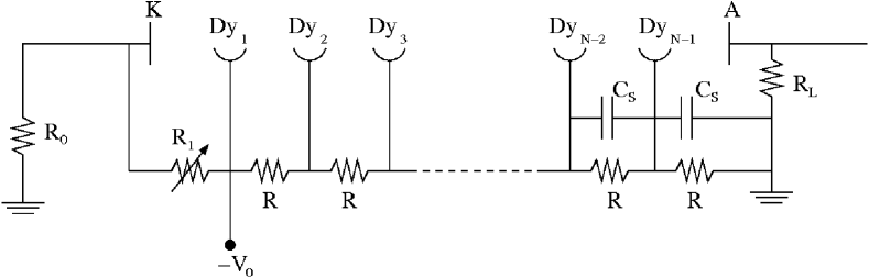
Figure 1: Electric scheme of the voltage divider of the Philips XP 2008 PMT used in the experiment. The photocathode is indicated with K, the anode with A and the various dynodes with Dy_i. The values of the resistances are $R_{0}=1\hbox{$\,{\rm M\Omega}$}$, $R=150\hbox{$\,{\rm k\Omega}$}$ and $R_{L}=100\hbox{$\,{\rm k\Omega}$}$. The resistance $R_{1}$ of the potentiometer connecting the cathode with the first dynode is allowed to vary in the range $[0,10]\hbox{$\,{\rm k\Omega}$}$. The capacitors in the last stages are used to keep the voltage differences stable, and their capacitance is $C_{S}=0.01\hbox{$\,{\rm nF}$}$.

Fig. 1 shows the electric scheme of the voltage divider used to provide the voltage differences to the dynodes. Unlike a standard PMT voltage divider, here the negative high voltage is supplied to the first dynode (not to the photocathode, which is grounded through the resistor $R_{0}$), thus ensuring that the photocathode K is kept at higher voltage with respect to the first dynode Dy1. The voltage difference between the two electrodes can be adjusted by changing the variable resistance $R_{1}$, and is given by:

$$V_{K}-V_{Dy1}=\frac{R_{1}V_{0}}{R_{0}+R_{1}}\approx\frac{R_{1}}{R_{0}}V_{0}.$$ (1)

In writing eq. 1 we took into account the fact that $R_{1}\ll R_{0}$ (see Fig. 1). If a high voltage $V_{0}=1000\hbox{$\,{\rm V}$}$ is supplied to the PMT, a maximum voltage difference of $10\hbox{$\,{\rm V}$}$ can be applied between K and Dy1. Since $V_{K}>V_{Dy1}$, photoelectrons extracted from K will be slowed down in their motion towards Dy1 and eventually sent back to K. On the other hand, like in standard PMT voltage dividers, the dynodes and the anode are kept at increasing potentials (if $V_{0}=1000\hbox{$\,{\rm V}$}$, the average voltage differences between each pair of dynodes will be of the order of $100\hbox{$\,{\rm V}$}$). In this way, photoelectrons eventually reaching Dy1 will be multiplied, producing a detectable current signal at the anode A, and consequently a voltage difference across the load resistor $R_{L}$.

LED	Peak wavelength ($\,{\rm nm}$)	Peak frequency ($\,{\rm 10^{14}Hz}$)
red	$631(17)$	$4.75(0.13)$
yellow	$585(15)$	$5.11(0.13)$
green	$563(12)$	$5.32(0.11)$
blue	$472(14)$	$6.34(0.18)$
violet	$403(6)$	$7.42(0.08)$

Table 1: Main features of the emission spectra of the LEDs used in the measurement. The wavelength and frequency spectra $(dN/d\nu\propto(1/\nu^{2})dN/d\lambda)$ have been fitted with gaussian functions. Here we report the mean values and, in brackets, the standard deviations of each fit function.

To perform our measurements we used five LEDs, emitting visible light of different colors ranging from red to violet. We preliminarily measured their emission spectra using an OCEAN OPTICS HR2000+ spectrometer ocean . Tab. 1 shows the peak values of the wavelengths and frequencies of each LED. The emission spectra of each LED have been fitted with gaussian functions. The values of the peak wavelengths (frequencies) and the corresponding standard deviations are reported in Tab. 1.

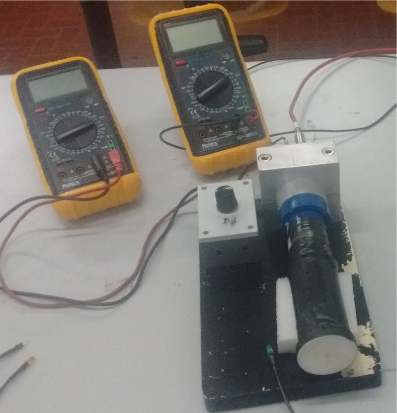
Figure 2: Photo of the experimental setup. The window of the photocathode is coupled to a plastic support with a hole drilled at its center, in which the different LEDs can be inserted. The PMT and the support are wrapped with black tape, to prevent external light entering in the device. Two digital multimeters are used to measure the voltage differences between the photocathode and the first dynode and across the load resistor. The knob on the left of the PMT is connected to a potentiometer, which allows to adjust the voltage of the first dynode.

Fig. 2 shows the experimental setup. The photocathode window is coupled to a plastic support with a hole drilled at its center where the different LEDs can be inserted. The PMT and the support are wrapped with black tape, to prevent external light entering into the device. The hole is also covered with black tape when a LED is inserted to perform a measurement. The voltage differences between K and Dy1 and across the load resistor $R_{L}$ are measured by two digital multimeters. The knob placed on the left of the PMT is connected to a potentiometer which allows the user to adjust the value of $R_{1}$ and consequently the voltage $V_{K}-V_{Dy1}$. The high voltage is supplied to the PMT by means of a CAEN N471A NIM power supply module caen (not shown in the figure). In our measurements we operated the PMT with high voltages in the range $700-1000\hbox{$\,{\rm V}$}$. This choice allows to keep a high PMT gain without incurring saturation effects due to large number of electrons flowing across the last dynodes.

The students should investigate the dependence of the voltage difference $V_{L}$ across the load resistor on the retarding potential $V_{R}=V_{K}-V_{Dy1}$ for the various LEDs. The value of $V_{L}$ is proportional to the anode current and consequently to the rate of photoelectrons collected by Dy1. During a measurement, the voltage across the LED must be kept constant, thus ensuring that the intensity of the light entering the PMT is also constant.

Photoelectrons extracted from the photocathode will have different initial kinetic energies up to a maximum value given by:

$$E_{K,max}=h\nu-W$$ (2)

where $h\nu$ is the energy of incident photons and $W$ is the work function of the photocathode. If $V_{R}=0$, all the photoelectrons extracted from K will be able to reach Dy1, and a current will flow through $R_{L}$. If $V_{R}$ is increased, only the more energetic photoelectrons will be collected by Dy1 and therefore the output current will decrease. When $eV_{R}\geq E_{K,max}$ the photoelectrons will not be allowed to reach Dy1 and the current flowing through $R_{L}$ is expected to vanish. The value

$$V_{S}=\frac{E_{K,max}}{e}=\frac{h\nu-W}{e}$$ (3)

represents the stopping potential, that depends on the energy of incident photons and on the work function of the photocathode.

From the plots of $V_{L}$ as a function of $V_{S}$ (hereafter we will refer to these plots as “photoelectric curves”), the students will be able to evaluate the stopping potential $V_{S}$ for each LED. The values of $V_{S}$ will then be plotted against the frequency $\nu$ of the incident light, and the data will be fitted with a straight line. According to equation 3, the value of $h/e$ will be derived from the slope of the line, while the value of $W/e$ will be derived from the intercept.

III Data analysis

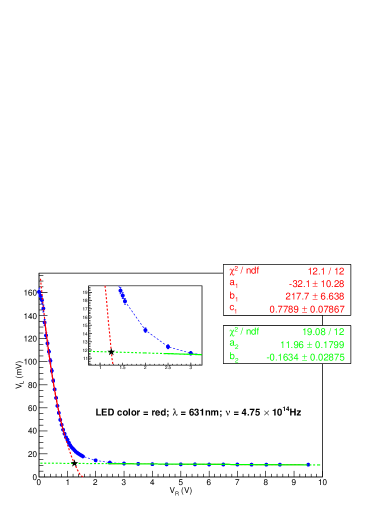
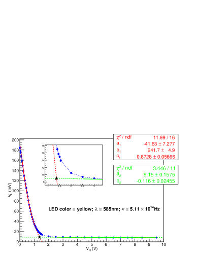
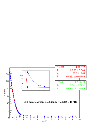
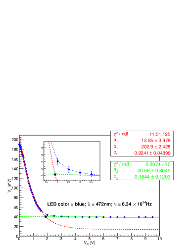
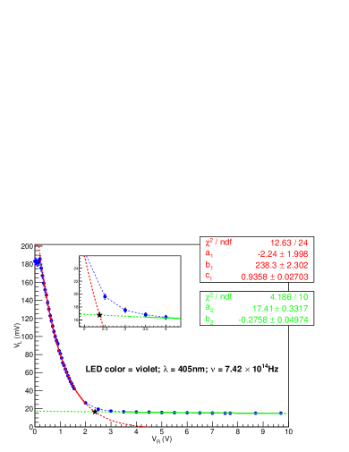
Figure 3: Examples of photoelectric curves obtained with the various LEDs. The continuous red and green lines represent the fits of the regions $V_{R}<V_{S}$ and $V_{R}>V_{S}$ with the two functions in eq. 4. The values of the fitted parameters and of the $\chi^{2}$ are shown in the top right panels of each plot, with the same color code. The dashed lines are obtained extrapolating the two fit functions outside the corresponding fit regions. A black star is drawn at the intersection point between the two fit functions. The abscissa of the intersection point provides the estimate of the stopping potential. A zoom of the region where the stopping potential is found is shown in the inset of each plot.

Fig. 3 shows some examples of photoelectric curves obtained when the PMT is illuminated with the various LEDs. As expected, the value of $V_{L}$ decreases with increasing $V_{R}$, but never drops to zero. This behavior can be explained by taking into account that a fraction of the incident photons can pass through the photocathode without interacting, and can extract photoelectrons from the first dynode. These electrons are accelerated towards Dy2, thus contributing to the output signal because of the high PMT gain. Hence, even when $V_{R}>V_{S}$, a background current will flow through the load resistor $R_{L}$, and consequently a steady positive value of $V_{L}$ will be measured. The fraction of photons extracting photoelectrons from the first dynode changes with the photon energy, as the absorption probabilities in the photocathode and in the first dynode are strongly dependent on the photon energy. Another possible contribution to the background anode current could be due to ambient light entering into the device, but we ruled out this contribution performing a preliminary set of measurements with the LEDs being turned off, in which we observed $V_{L}=0$ for any value of $V_{R}$. Finally, it is also worth to point out here that the electron optics of a PMT is designed for electrodes kept at increasing potentials. Therefore electrons emitted from the photocathode are accelerated towards the first dynode and are focused onto its center regardless their emission angle, thus ensuring optimal collection efficiency. Setting in our device a retarding potential between K and Dy1, we introduce a distortion in the electron optics of the PMT, that affects the trajectories of photoelectrons preventing them to reach the first dynode. However, even when $V_{R}>V_{S}$, some photoelectrons travelling in weaker field regions might be able to reach the first dynode, contributing to the output signal.

We performed several sets of measurements, changing either the high voltage $V_{0}$ supplied to the PMT or the intensity of the light emitted by the various LEDs. An increase of $V_{0}$ will result in an increase of the gain of the electron multiplier, while an increase of the light intensity will result in an increase of the number of photoelectrons. In particular, we observe that, if the light intensity is kept constant and $V_{0}$ is changed, the shape of the photoelectric curves does not change, but the values of $V_{L}$ corresponding to a given $V_{R}$ increase with increasing $V_{0}$. Similarly, if $V_{0}$ is kept constant and the light intensity is changed, the shape of the photoelectric curves does not change, but the values of $V_{L}$ increase with increasing light intensity. This behavior is observed for a wide range of high voltages ($V_{0}\sim 700\div 1100\hbox{$\,{\rm V}$}$) and LED intensities (here the range depends on the color of the LEDs). However, if the voltage across the load resistor becomes too large ($V_{L}\gtrsim 1\hbox{$\,{\rm V}$}$), saturation effects might occur due to the large number of electrons moving across the last dynodes because the capacitors in the last stages of the voltage divider could not be able to keep the voltage differences stable.

Another feature of the photoelectric curves shown in Fig. 3 is that the transition between the regime in which photoelectrons emitted from K are collected by Dy1 and the regime in which photoelectrons are repelled is not sharp, i.e. the slope of the photoelectric curve changes smoothly with $V_{R}$, thus making the determination of $V_{S}$ not straightforward. This behavior is due to the spread in the photoelectron kinetic energies when they are emitted from the photocathode. It is also worth to point out here that, since photons emitted by LEDs are not monochromatic (as shown in Tab. 1 the widths of the frequency spectra are $\sim 2\div 3\%$ of the corresponding peak values), the photoelectric curves cannot be described in terms of a single value of the stopping potential, but it would be more appropriate to take into account the dependence of the stopping potential on the frequency. Hereafter we will neglect this depencence and we will assume that each photoelectric curve can be described in terms of the stopping potential $V_{S}$ corresponding to the peak frequency of the LED.

The determination of either an analytical or a numerical model of the photoelectric curves would be rather complex and perhaps would go beyond the scope of an introductory laboratory course for undergraduate students. Therefore, to analyze the data collected by the students carrying out the experiment, we developed a phenomenological approach. After the analysis of many photoelectric curves obtained in different conditions (different LED intensities and different PMT high voltages), we noticed that the asymptotic behavior of all photoelectric curves can be adequately described by the following functions:

$$V_{L}=\left\{\begin{array}[]{ll}a_{1}+b_{1}e^{-\frac{V_{R}}{c_{1}}}&\textrm{for}~{}V_{R}<V_{S}\\ a_{2}+b_{2}V_{R}&\textrm{for}~{}V_{R}>V_{S}\\ \end{array}\right.$$ (4)

For each photoelectric curve we select two sets of points, belonging to the regions $V_{R}<V_{S}$ and $V_{R}>V_{S}$, and we fit these points with the functions in eq. 4, thus determining the parameters $a_{1}$, $b_{1}$, $c_{1}$, $a_{2}$ and $b_{2}$. The fits are performed using the free data analysis software ROOT root , provided by CERN. We then define the value of the stopping potential $V_{S}$ as the abscissa of the intersection point of the two curves, which can be evaluated solving the following non-linear equation:

$$a_{1}+b_{1}e^{-\frac{V_{S}}{c_{1}}}=a_{2}+b_{2}V_{S}.$$ (5)

The previous equation, which gives $V_{S}$ as a function of the parameters $a_{1}$, $b_{1}$, $c_{1}$, $a_{2}$ and $b_{2}$, cannot be solved analytically, but can be easily solved in a numerical way, for instance using the bisection method. This procedure is graphically illustrated in the plots of Fig. 3, where we superimposed to each photoelectric curve the functions obtained from the two fits, also showing the position of the intersection between the two curves. As we anticipated in Sec. I, it is worth to point out here that the detection of a significant steady background current instead of a slowly vanishing current helps to better define the stopping potential.

To evaluate the error on $V_{S}$ we use the standard error propagation formula, starting from the errors on $a_{1}$, $b_{1}$, $c_{1}$, $a_{2}$ and $b_{2}$, which are computed by the ROOT software when performing the fits. However, since $V_{S}$ is an implicit function of the parameters, a numerical approach is also needed to evaluate its partial derivatives with respect to the various parameters. For instance, to evaluate the partial derivative $\partial V_{S}/\partial a_{1}$, we start from the set of fitted parameters and we change $a_{1}$ into $a_{1}^{\prime}=a_{1}+\delta a_{1}$ ; then we solve eq. 5 with the value of $a_{1}^{\prime}$, obtaining a new solution $V_{S}^{\prime}$ and finally we evaluate the partial derivative as $\partial V_{S}/\partial a_{1}\approx\delta V_{S}/\delta a_{1}$, where $\delta V_{S}=V_{S}^{\prime}-V_{S}$. In the same way we calculate the partial derivatives of $V_{S}$ with respect to the other parameters.

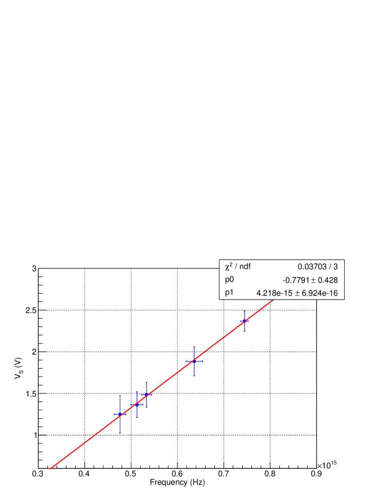
Figure 4: Stopping potentials for the various LEDs as a function of frequency. The horizontal error bars represent the width of the spectra shown in Tab. 1, while the vertical error bars represent the uncertainties on the stopping potentials, evaluated as discussed in sec. III. The points are well fitted with a straight line. The fit results are summarized in the top panel (the parameters $p_{0}$ and $p_{1}$ are respectively the intercept the slope), where the $\chi^{2}$ of the fit is also shown.

The procedure used to evaluate $h/e$ from the measured stopping potentials is illustrated in Fig. 4, where the stopping potentials obtained from the analysis of the photoelectric curves shown in Fig. 3 are plotted against the frequency of the incident light. The error bars associated to the LED frequencies are the widths of their emission spectra, which are taken from Tab. 1, while those associated to the stopping potentials are calculated following the approach described above. A linear fit of the experimental points is then performed. In the example shown in Fig. 4, the fit procedure yields a $\chi^{2}/d.o.f.=0.037/3$, which suggests that the error bars associated to the stopping potentials are overestimated, a feature which might be a consequence of the phenomenological model that we adopted to describe the photoelectric curves. According to eq. 3, the slope of the line corresponds to $h/e$, while its intercept corresponds to $W/e$. Assuming for the electron charge the current value $e=1.60\times 10^{-19}\hbox{$\,{\rm C}$}$, the fit of the data shown in Fig. 4 yields for the Planck’s constant a value $h=(6.75\pm 1.11)\times 10^{-34}\hbox{$\,{\rm J\cdot s}$}$ and for the work function of the photocathode a value $W=(0.78\pm 0.43)\hbox{$\,{\rm eV}$}$.

IV Discussion and conclusions

The measurement of $h/e$ proposed in the present paper yields an uncertainty of about $20\%$ on the value of $h/e$ and an uncertainty larger than $50\%$ on $W/e$. The main sources of error are the spreads on the LED frequencies and the uncertainties on the values of the stopping potentials. To mitigate the effects of the frequency spreads, one could use monochromatic light sources coupling the LEDs to appropriate filters, or even using laser sources. The uncertainties on the stopping potentials could also be reduced with a more appropriate modeling of the photoelectric curves, which goes beyond the scope of an introductory laboratory course.

Despite the poor precision attained, we strongly believe that this measurement of $h/e$ is extremely useful from the educational point of view, because not only it allows to understand the main features of the photoelectric effect, but it also stimulates further considerations about the physics involved in the measurement and on the technique adopted.

References

- (1) M. Planck, “On the distribution law of energy in the normal spectrum”, Annalen der Physik IV, 7, 553-563 (1901).
- (2) A. Einstein, “On a Heuristic Point of View about the Creation and Conversion of Light”, Annalen der Physik 17, 6, 132–148 (1905).
- (3) S. George et al., “Planck’s Constant from Wien’s Displacement Law”, AJP 40, 621 (1972).
- (4) C. N. Manikopoulos and J. F. Aquirre, “Determination of the blackbody radiation constant hc/k in the modern physics Laboratory”, AJP 45, 576 (1977).
- (5) R. E. Crandall and J. F. Delord, “Minimal apparatus for determination of Planck’s constant”, AJP 51, 90 (1983).
- (6) J. Dryzek and K. Ruebenbauer, “Planck’s constant determination from black‐body radiation”, AJP 60, 251 (1992).
- (7) G. Brizuela and A. Juan, “Planck’s constant determination using a light bulb”, AJP 64, 819 (1996).
- (8) L. Nieves et al., “Measuring the Planck constant with LED’s”, The Physics Teacher 35, 108 (1997).
- (9) A. J. O’Leary, “Two Elementary Experiments to Demonstrate the Photoelectric Law and Measure the Planck Constant”, AJP 14, 245 (1946).
- (10) H. Hall and R. P. Tuttle, “Photoelectric Effect and Planck’s Constant in the Introductory Laboratory”, AJP 39, 50 (1971).
- (11) R. L. Bobst and E. A. Karlow, “A direct potential measurement in the photoelectric effect experiment”, AJP 53, 911 (1985).
- (12) J. Dean Barnett and H. T. Stokes, “Improved student laboratory on the measurement of Planck’s constant using the photoelectric effect”, AJP 56, 86 (1988).
- (13) W. P. Garver, “The Photoelectric Effect Using LEDs as Light Sources”, The Physics Teacher 44, 272 (2006).
- (14) R. A. Millikan, “A direct photoelectric determination of Planck’s h”, Phys. Rev. 7, 355-388 (1916).
- (15) R. A. Millikan, “The isolation of an ion, a precision measurement of its charge, and the correction of Stokes’s law”, Phys. Rev. (Series I) 32, 349-397 (1911).
- (16) R. A. Millikan,“On the Elementary Electrical Charge and The Avogadro Constant”, Phys. Rev. 2, 109-143 (1913).
- (17) Philips Photomultipliers: Data Handbook, PC04 (1990).
- (18) http://www.oceanoptics.com/Products/benchoptions_hr.asp
- (19) http://www.caen.it/csite/CaenProd.jsp?parent=21&idmod=240
- (20) https://root.cern.ch/ see also R. Brun and F. Rademakers, “ROOT - An Object Oriented Data Analysis Framework”, Proceedings AIHENP’96 Workshop, Lausanne, Sep. 1996, Nucl. Inst. & Meth. in Phys. Res. A 389, 81-86 (1997).
- (21) G. F. Knoll, “Radiation Detection and Measurement”, Wiley (1999).