Weakly Learning to Match Experts in Online Community

Abstract

In online question-and-answer (QA) websites like Quora, one central issue is to find (invite) users who are able to provide answers to a given question and at the same time would be unlikely to say “no” to the invitation. The challenge is how to trade off the matching degree between users’ expertise and the question topic, and the likelihood of positive response from the invited users. In this paper, we formally formulate the problem and develop a weakly supervised factor graph (WeakFG) model to address the problem. The model explicitly captures expertise matching degree between questions and users. To model the likelihood that an invited user is willing to answer a specific question, we incorporate a set of correlations based on social identity theory into the WeakFG model. We use two different genres of datasets: QA-Expert and Paper-Reviewer, to validate the proposed model. Our experimental results show that the proposed model can significantly outperform (+1.5-10.7% by MAP) the state-of-the-art algorithms for matching users (experts) with community questions. We have also developed an online system to further demonstrate the advantages of the proposed method.

1 Introduction

Led by technology innovation, the global economy is in transition to a “knowledge economy”. It is common to post a question on knowledge sharing or question-and-answer websites such as Quora and invite “experts” to help answer the question. Thus, finding appropriate experts for the given question becomes a central task. In the past, related research including experts finding for community-based questions Riahi et al. (2012); Zhao et al. (2015), peer reviewer recommendations for papers Deng et al. (2008); Djupe (2015); Dumais and Nielsen (1992); Goldsmith and Sloan (2007); Long et al. (2013); Tang et al. (2012), and expertise modeling Han et al. (2016); Mimno and McCallum (2007); Zhang et al. (2007) has been conducted. A survey can be also found in Balog et al. (2012). However, most existing research does not consider the second half of the problem — the probability of whether the invited experts would accept to answer the question. Indeed, the subproblem is even more serious—e.g. more than half of the questions on Quora only have one or do not have any answer.

These QA websites such as Quora are now striving to match questions with the right experts and seek the best respondent to provide an answer. The problem can be formalized as follows: Given a query (i.e., question/document) $q$, one of the goals is to find experts with sufficient knowledge. We consider a set of $N$ candidate experts $E=\{e_{1},\cdots,e_{N}\}$. We use function $R(q,e_{i})$ to measure the extent to which expert $e_{i}$ has the knowledge on query $q$. The other goal here is to estimate how likely expert $e_{i}$ would accept to answer the query $q$. We use function $R^{\prime}(q,e_{i})$ to quantify the probability of acceptance. Finally, the above problem can be defined as: given a query $q$ and a set of experts $E=\{e_{1},\cdots,e_{N}\}$, the goal is to maximize the utility function:

$$S_{qi}=\alpha R(q,e_{i})+(1-\alpha)R^{\prime}(q,e_{i})$$ (1)

where $\alpha$ is a tunable parameter to trade off the importance between the matching degree of expert $e_{i}$ with query $q$ and the acceptance probability of expert $e_{i}$ to answer $q$. Setting $\alpha=1$ would reduce the problem to the traditional expert finding problem without considering the acceptance probability of the invited expert.

The problem defined in Eq. (1) is much more challenging than the traditional expert finding problem. This is because factors that affect an expert to accept (or reject) an answer invitation are very complicated. For example, it might be because the expert is overloaded or simply due to the unpopularity of the topic. Moreover, how to instantiate the function $R^{\prime}(q,e_{i})$ in oder to quantify the acceptance probability is another challenge. From the algorithm perspective, we can feed some training data to a machine learning algorithm to learn a predictive model; however, the trouble is how to collect sufficiently labeled data. The last challenge is how to evaluate the performance of a potential solution, in particular in an online fashion.

Our Solution and Contributions. In this paper, we formalize the problem into a weakly supervised factor graph (WeakFG) model to address the aforementioned challenges. We introduce embedding-based metrics to measure the matching degree between queries and experts. WeakFG is able to learn from response logs to predict who are more likely to accept/decline an answer invitation. To address the problem of lacking labeled data, WeakFG defines a set of correlation functions and uses the correlations to propagate the labeled information to unlabeled data.

To validate the effectiveness of the proposed model, we conduct both offline and online evaluations. For the offline evaluation, we first use the data from an international competition in 2016. The task is to predict the probability that an expert answers a given question in online communities. Experimental results show that the proposed model can achieve better performance (1.5-10.7% by MAP) than several state-of-the-art algorithms. To validate the generality of the proposed model, we applied it to a related, but somehow different, setting: peer-reviewer recommendation — recommending reviewers to scientific articles. We use the bidding information of a major computer science conference with $\sim 1,000$ submissions and $440$ program committee members to evaluate the prediction on acceptance of review invitation. We achieve the same better performance than several comparison methods. For online evaluation, we developed a Chrome Extension of reviewer recommendation and deployed it in the Google Chrome Web Store. About 50 journal editors downloaded the extension and used it for reviewer recommendations. Feedbacks from users also demonstrate the effectiveness of the proposed method.

2 Related Work

Related research can be traced back to 30 years ago. We briefly survey existing literature from three aspects: expert finding, expert matching, and expertise modeling.

Expert finding aims to identify experts for given topic/query. Applications include finding experts to answer question in online communities Liu et al. (2005); Riahi et al. (2012); Zhao et al. (2015), finding experts to review scientific articles Yang et al. (2009); Djupe (2015); Haym et al. (1999), finding experts from bibliography data Deng et al. (2008); Zhang et al. (2008), or finding software developers to fix a bug Xia et al. (2017). This category of research is closely related to our work. Those methods can be used to instantiate the left term in Eq. (1). The second category of related research is expert matching. The goal is to assign a list of experts to a list of queries by considering matching degree, load balance, and other constraints. There was a bunch of research on this topic, probably starting from conference-paper-reviewer assignment Benferhat and Lang (2001); Dumais and Nielsen (1992); Goldsmith and Sloan (2007); Karimzadehgan and Zhai (2009); Kou et al. (2015); Long et al. (2013); Tang et al. (2012) to recently studies for online community and crowdsourcing Hung et al. (2015). One problem which has long been criticized Ishiyama (2014, 2015) in expert matching is that it does not consider the expert’s willingness likelihood, i.e., the second term in Eq. (1). The study of expertise modeling focuses on mining experts’ interests or expertise. Methods using probabilistic model Mimno and McCallum (2007), network analysis Zhang et al. (2007), and embedding Han et al. (2016) have been developed. However, they did not consider the experts’ acceptance probability.

A few systems have been developed to make reviewer recommendations, e.g., AMiner Tang et al. (2008). Toutiao organized a data challenge to predict the probability that an expert would accept the invitation to answer specific questions.

Figure 1: Decline probability of an expert conditioned on whether or not the expert has a correlated “friend” who has already declined on two datasets: QA-Expert and Paper-Reviewer, and our online evaluation of journal reviewer recommendation.

3 Methodologies

Given a query (e.g., question/paper) $q$, our goal is to find experts with sufficient knowledge who are willing to answer the question or review the paper, with limited amount of labeled data. Let us consider a set of $N$ candidate experts $E=\{e_{1},\cdots,e_{N}\}$. The general problem can be then formalized as seeking a ranking function to quantify each expert $e_{i}$’s expertise degree and acceptance probability simultaneously.

The ranking score $S_{qi}$ was defined by only considering the expertise matching degree between $q$ and the expert $e_{i}$ (Cf. the first term in Eq. (1)). One method is to use language models Zhai and Lafferty (2001), which estimates the generative probability of a query given each document (expert-related document here) using a smoothed word distribution. Afterwards, topic models have been used to model latent topics in order to improve the matching accuracy Mimno and McCallum (2007); Riahi et al. (2012); Tang et al. (2008).

However, all these models do not consider the probability that expert $e_{i}$ accepts to answer the query $q$. Algorithmically, the difficulty is how to define the second term in Eq. (1). Another challenge, in practical scenarios, is the lack of sufficient labeled data. One potential solution to this end is weakly supervised learning Crandall and Huttenlocher (2006), which essentially leverages some kind of correlation between training instances to propagate the labeled information to unlabeled instances. Widely used correlations include similarity and links (e.g., friend or coauthor relationships). Figure 1 shows the decline probability of an expert, conditioned on whether or not the expert has a “friend” who has already declined. We see correlation indeed exists in all the datasets used in our experiments (Cf. §4 for details of the datasets).

Now, finding useful correlations becomes an important issue. Social relationships like friendships can be considered as correlations, but are still sparse. We present an interesting idea of defining correlations using social identify theory Turner and Oakes (1986); Tajfel and Turner (2004), which suggests that people with the same social identity (e.g., position, affiliation, age, etc.) tend to share the same social behavior. For example, in an online community, users with the same job tend to accept/decline the same question invitation; in the paper-reviewer recommendation setting, researchers from the same organization are more likely to decline an invitation at the same time. We formalize the social identify-based correlations into a weakly supervised factor graph (WeakFG) model, to simultaneously learn the expertise matching degree and the acceptance probability with limited labeled data.

3.1 WeakFG: Weakly Supervised Factor Graph

We now explain how WeakFG works. In WeakFG, we first use the embedding technologies Mikolov et al. (2013) to capture semantics of expertise matching and then use a semi-supervised graph model to predict whether expert $e_{i}$ will accept or decline an invitation, by considering both local similarity and correlation between experts.

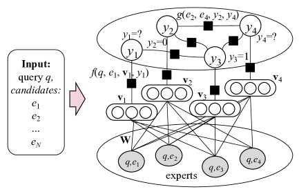
Figure 2: Graphical representation of the WeakFG model. Variable $y_{i}$ indicates whether expert $e_{i}$ declines the invitation; $\textbf{v}_{i}$ indicates the embedding for expert $e_{i}$; $f(q,e_{i},\textbf{v}_{i},y_{i})$ and $g(e_{i},e_{j},y_{i},y_{j})$ represent the local factor function defined for expert $e_{i}$ on query $q$, and the correlation factor function defined between experts $e_{i}$ and $e_{j}$.

An example is illustrated in Figure 2. Given a query $q$ and candidate experts $\{e_{1},e_{2},e_{3},e_{4}\}$, we first generate the embedding-based representation for each expert, i.e., $\{\textbf{v}_{1},\textbf{v}_{2},\textbf{v}_{3},\textbf{v}_{4}\}$. A factor graph is then constructed by defining local factor function $f(q,e_{i},\textbf{v}_{i},y_{i})$ to capture local attributes of each query-expert pair, and correlation factor function $g(e_{i},e_{j},y_{i},y_{j})$ to capture potential correlation between different experts. Variable $y_{i}$ indicates whether expert $e_{i}$ accepts (=0) the invitation or declines (=1) it. For example, in Figure 2, expert $e_{3}$ has a correlation with each other expert. For training the factor graph model, we have two labeled instances ($y_{2}=0$ and $y_{3}=1$), thus our goal is to infer the other two unlabeled instances ($y_{1}$ and $y_{4}$).

It should be noted that each observation node $e_{i}$ in WeakFG actually encodes information related to both query $q$ and $e_{i}$. Essentially, the local factor function $f(q,e_{i},\textbf{v}_{i},y_{i})$ aims to model the expertise matching degree, while the correlation factor function aims to propagate the labeled information in the graph in order to help infer acceptance probabilities of unlabeled instances. Now we introduce how we calculate the expertise matching degree, and explain how we instantiate the factor functions in WeakFG.

Expertise Matching. We define local factor functions to capture the expertise matching degree between expert and query. Given a query $q$ and an expert $e$, we calculate the expertise matching score $R(q,e)$. The matching score can be defined based on various methods. For example, one can use the keyword based model, e.g., vector-space model or language model Zhai and Lafferty (2001). To further capture the semantic information, we can use the recently developed embedding method Mikolov et al. (2013), which has shown promising results in many fields such as natural language processing, image processing, and speech recognition.

More specifically, a query $q$ can be considered as a document, and an expert $e$ can be considered as a document set $\{d_{k}\},k\in\{1,\cdots,N_{e}\}$, where each $d_{k}$ represents a document authored by $e$, e.g., an answer provided by $e$ or a paper published by $e$. We define the expertise matching score $R(q,e)$ as the similarity between query document $q$ and the document set $\{d_{k}\}$,

$$R(q,e)=\bigoplus_{k\in\{1,\cdots,N_{e}\}}\mathrm{Sim}(q,d_{k})$$ (2)

where $\bigoplus$ is an aggregation function, e.g., $max$ or $avg$.

We use embedding to calculate the similarity between query $q$ and document $d_{k}$, i.e., $\mathrm{Sim}(q,d_{k})$. To do this, we first learn a numeric vector representation (i.e., word embedding) for each word. We use Word2Vec with Skip-gram Mikolov et al. (2013) to learn the word embeddings. Word2Vec is a shallow neural network architecture consisting of an input layer, a projection layer, and an output layer. The training objective is to use an input word $w$ to predict surrounding words in its context. After the embedding training, we obtain an embedding vector $\mathbf{v}_{w}$ for each word $w$. Then we estimate $\mathrm{Sim}(q,d_{k})$ using two embedding-based algorithms: WMD and D2V.

Word Mover’s Distance (WMD). WMD is a distance function Kusner et al. (2015). Specifically, each document $d$ can be represented as a normalized bag-of-words (nBOW) vector $\boldsymbol{\tau}\in\mathbb{R}^{n}$, with each element $\boldsymbol{\tau}_{i}=\frac{\mathcal{N}^{i}_{d}}{{\sum_{j=1}^{n}\mathcal{N}^{j}_{d}}}$ standing for the weight of word $i$ and $\mathcal{N}^{i}_{d}$ indicating the occurrence times of word $i$ in the document. The similarity between documents $q$ and $d$ can be defined by the following linear program,

$$\small\begin{split}&\mathrm{Sim}_{\mathrm{WMD}}(q,d)=-\min_{\mathbf{W}_{ij}\geq 0}\sum_{i=1}^{n}\sum_{j=1}^{n}\mathbf{W}_{ij}\|\mathbf{v}_{i}-\mathbf{v}_{j}\|_{2}\\ &\text{s.t. }\sum_{j=1}^{n}\mathbf{W}_{ij}=\boldsymbol{\tau}_{i}^{q},\ \sum_{i=1}^{n}\mathbf{W}_{ij}=\boldsymbol{\tau}_{j}^{d},\ \forall i,j\in\{1,\dots,n\}\end{split}\normalsize$$ (3)

where the linear program aims to find an optimal matching between words in $q$ and those in $d$; $\boldsymbol{\tau}^{q}$ and $\boldsymbol{\tau}^{d}$ are the nBOW vectors for $q$ and $d$. Mathematically, each word $w_{i}$ in $q$ can be matched to any word $w_{j}$ in $d$ with the weight $\mathbf{W}_{ij}$. The distance between two specific words is defined as Euclidean distance $\|\cdot\|_{2}$ of their embeddings $\mathbf{v}_{i}$ and $\mathbf{v}_{j}$. We use the negative value of the distance as the similarity.

Document Vector (D2V). D2V aims to directly learn an embedding vector for each document. The document vectors can be learned by predicting all words in the document Le and Mikolov (2014). In this paper, we use the distributed bag of words idea. Specifically, given a document, we use stochastic gradient descent to learn the embedding vector, where in each iteration we sample a random word from the context and predict the word with the embedding vector. For the prediction, we use the softmax function:

$$p(w|d)=\frac{\exp\left({\mathbf{v}_{w}}^{\top}\mathbf{\hat{v}}_{d}\right)}{\sum_{w^{\prime}=1}^{n}\exp\left({\mathbf{v}_{w^{\prime}}}^{\top}\mathbf{\hat{v}}_{d}\right)}$$

where $\mathbf{\hat{v}}_{d}$ indicates the document vector and $\mathbf{v}_{w}$ indicates the word vector. After learning the document vectors, the similarity between documents $q$ and $d$ can be defined as:

$$\mathrm{Sim}_{\mathrm{D2V}}(q,d)=\frac{{\mathbf{\hat{v}}_{q}}{{}^{\top}}\mathbf{\hat{v}}_{d}}{\|\mathbf{\hat{v}}_{q}\|_{2}\cdot\|\mathbf{\hat{v}}_{d}\|_{2}}$$ (4)

WeakFG Formalization. Based on the learned embeddings (by either WMD or D2V), we estimate the expertise matching scores between query and experts, and then construct the WeakFG model by defining Local factor function and Correlation factor function.

Local factor function: It captures any attributes for each query-expert pair, including expertise matching score between the query and the expert, and any other attributes associated with them. We define local factor as

$$f(q,e_{i},\textbf{v}_{i},y_{i})=\exp\left\{{\boldsymbol{\alpha}_{y_{i}}}^{\top}\boldsymbol{\psi}(q,\textbf{v}_{i},e_{i})\right\}$$ (5)

where $\boldsymbol{\psi}(.)$ is a set of feature functions defined for $q$ and $e_{i}$. For example, a potential function $\psi(.)$ can be defined as the expertise matching score $R(q,e_{i})$ (Eq. (2)). $\boldsymbol{\alpha}=(\boldsymbol{\alpha}_{0}^{\top},\boldsymbol{\alpha}_{1}^{\top})^{\top}$ is the weight vector of the defined features.

We can define domain-specific statistics as feature functions for each candidate expert. For example, in the QA expert finding task, we can define the number of questions answered by the expert as a feature, while in the paper-reviewer recommendation task, we can define features based on the expert’s $h$-index, position, publication number, and citation number. The feature functions can be either binary or real-valued.

Correlation factor function: The correlation between experts can be used to help infer experts’ acceptance probability. It is modeled as correlation factor functions among latent variables $\{y_{i}\}$. Formally, it can be also defined as:

$$g(e_{i},e_{j},y_{i},y_{j})=\exp\{{\boldsymbol{\beta}_{y_{i},y_{j}}}^{\top}\boldsymbol{\phi}(e_{i},e_{j})\}$$ (6)

where $\boldsymbol{\phi}(.)$ is a set of indicator functions to model whether specific correlation exists between experts $e_{i}$ and $e_{j}$; $\boldsymbol{\beta}$ indicates the weights of different factors.

In different applications, there are different types of correlations between experts. For example, in QA expert finding, we can define correlation as co-reply, corresponding to the situation when two users have replied to the same question. In paper-reviewer recommendation, we can consider co-author relationship. However, as shown in Figure 1, such kinds of correlations might be still insufficient. We further define some other social identity Tajfel and Turner (2004) based correlations. Social identity theory introduced a way to explain intergroup behavior, in particular to predict certain intergroup behavior on the basis of the perceived group status difference. For example, in the QA expert finding task, users of the same position (e.g., CFO) may tend to decline the same question, e.g., about specific technique. For correlation factors, we use binary functions, i.e., $\phi_{l}(e_{i},e_{j})=1$ if and only if a specific correlation exists.

Objective Function. Let $G$ denote all the observation variables, including the experts and their relations, and $Y=\{y_{1},\dots,y_{N}\}$ denote the latent variables. We define the joint probability of latent variables conditioned on the observations by integrating the two factor functions:

$$\small\begin{split}&P(Y|G)=\frac{1}{Z}\prod_{e_{i}}f(q,e_{i},\textbf{v}_{i},y_{i})\prod_{(e_{i},e_{j})}g(e_{i},e_{j},y_{i},y_{j})\\ &=\frac{1}{Z}\exp(\sum_{e_{i}}{\boldsymbol{\alpha}_{y_{i}}}^{\top}\boldsymbol{\psi}(q,\textbf{v}_{i},e_{i})+\sum_{(e_{i},e_{j})}{\boldsymbol{\beta}_{y_{i},y_{j}}}^{\top}\boldsymbol{\phi}(e_{i},e_{j}))\end{split}$$ (7)

where $Z$ is a normalization factor to ensure $\sum_{Y}P(Y|G)=1$; and $\boldsymbol{\theta}=\{\boldsymbol{\alpha},\boldsymbol{\beta}\}$ are the model parameters to estimate.

3.2 Model Learning

We now discuss how to estimate the model parameters $\boldsymbol{\theta}=\{\boldsymbol{\alpha},\boldsymbol{\beta}\}$ in WeakFG. Our goal is to find a parameter configuration $\boldsymbol{\theta}$ from a given training dataset $(\tilde{Y},G)$, such that the log-likelihood objective function $L(\boldsymbol{\theta})=\log P(\tilde{Y}|G)$ can be maximized, i.e.,

$$\boldsymbol{\theta}^{*}=\arg\max_{\boldsymbol{\theta}}\log P(\tilde{Y}|G)$$ (8)

The optimization can be solved using a gradient ascent algorithm. As an example, we derive the gradient of $\boldsymbol{\alpha}_{0}$ (the gradients of other parameters can be derived analogously):

$$\frac{\partial L(\boldsymbol{\theta})}{\partial\boldsymbol{\alpha}_{0}}=\sum_{e_{i}}\boldsymbol{\psi}(q,\textbf{v}_{i},e_{i})\cdot\left[\mathbb{1}(\tilde{y}_{i}=0)-P(y_{i}=0|G)\right]$$ (9)

where $\mathbb{1}(\tilde{y}_{i}=0)$ is an indicator function which equals to $1$ if the label $\tilde{y}_{i}=0$, and $0$ otherwise. The above gradient is intractable due to the difficulty to determine the marginal probability $P(y_{i}|G)$. There are several approximation methods. In our work, we choose Loop Belief Propagation (LBP) Yedidia et al. (2000). We first derive a factor graph from the original graph $G$, representing the factorization of the likelihood $P(Y|G)$. In each iteration, LBP performs message passing on the factor graph based on sum-product algorithm Kschischang et al. (2001), and compute the approximate marginal distributions. Then we compute the gradients and update the parameters with learning rate $\eta$.

Prediction. Given the input network $G$ and the parameters $\boldsymbol{\theta}$, the prediction task is to find the most likely configuration $Y_{q}$ for a given query $q$, i.e., $Y_{q}=\arg\max_{Y}P(Y|G).$

For prediction, we use the max-sum algorithm to find the values of $Y_{q}$ that maximize the likelihood. The max-sum algorithm is similar to the sum-product algorithm, except for calculating the message according to $max$ instead of $sum$ in message passing functions.

Candidate Generation. Finally, we discuss a bit about the candidate generation, as it does matter in real applications. When looking for experts for a query, we would first select candidate experts by a coarse-level matching algorithm. This is necessary to reduce the computational cost. Specifically, given a query $q$, we use all words in the query to select candidate experts. We use language model (LM) to retrieve relevant experts from $V$. LM interprets the relevance between a document and a query word as a generative probability $p(w|d)$. For details, please refer to Zhai and Lafferty (2001).

4 Experiments

We performed both offline and online evaluations to demonstrate the effectiveness of the proposed model. The code for this paper is publicly available.

Table 1: Performance comparison of different methods.

		QA-Expert					Paper-Reviewer
Method		P@1	P@3	P@5	MAP	Rprec	P@3	P@5	P@10	MAP	Rprec
LM	max	36.8	34.9	33.2	57.4	55.7	66.5	61.6	54.7	76.7	67.2
	avg	37.5	36.8	33.2	57.9	55.6	69.9	63.3	54.9	78.2	68.3
BM25	max	33.6	33.6	33.3	55.1	53.5	67.1	61.8	54.8	77.0	67.1
	avg	41.4	34.6	33.3	59.1	56.5	70.2	63.9	55.1	78.1	68.4
LDA	max	37.5	35.3	33.2	56.7	53.9	63.0	59.3	54.1	72.8	65.6
	avg	32.9	33.8	32.9	53.6	51.4	66.3	62.6	55.2	75.8	67.9
WMD	max	40.8	36.4	34.0	59.5	56.2	67.3	61.5	54.6	76.3	67.2
	avg	38.2	38.2	34.1	58.8	55.6	64.2	59.3	53.0	73.7	63.5
D2V	max	36.2	34.4	33.2	57.3	55.6	69.6	62.5	55.1	77.7	68.3
	avg	29.6	32.7	33.3	53.9	53.0	72.3	65.4	56.2	80.5	71.3
RankSVM		49.8	38.5	33.7	65.5	63.1	70.6	64.8	56.0	81.0	72.7
WeakFG		52.8	39.6	34.1	67.4	64.5	71.9	65.5	56.3	82.0	73.8

4.1 Experimental Setup

Datasets. We conducted experiments on two datasets.

QA-Expert: this dataset is from an online international QA challenge${}^{\text{2}}$.  It consists of 87,988 users and 47,656 questions with 43,913 invitations and 9,561 responses. To reduce noise, we select those questions with at least 5 invited users and 1 response in our experiment. This results in 182 questions and 599 users. In this dataset, we aim to evaluate how can our method improve the performance of predicting users’ responses to answer invitations in the online QA system.

Paper-Reviewer: this dataset comes from the reviewer bidding of a major CS conference in 2016. It contains 935 submissions and 440 Program Committee members. PC members placed bids for the papers they are interested to review. For each paper, we consider PC’s bids as a positive response to the invitation, and randomly sample the same number of PCs who do not bid for this paper as negative.

In each dataset, we randomly select 60% as the training data and the remaining as test data. We perform experiments on each dataset for 10 times and report the average results.

Comparison Methods. We compare the following methods:

Language Model (LM) Zhai and Lafferty (2001): We employ language model to calculate the document similarity. We compare $max$ and $avg$ to derive $R(q,e)$ in the experiments.

BM25 Robertson et al. (2009): A widely used ranking function in information retrieval. The similarity score is defined as

$$\mathrm{Sim}(q,d)=\sum_{w\in q}\mathit{IDF}(w)\cdot\frac{\mathcal{N}_{d}^{w}\cdot(k_{1}+1)}{\mathcal{N}_{d}^{w}+k_{1}\cdot(1-b+b\cdot\frac{\mathcal{N}_{d}}{\lambda})}$$

where $\mathit{IDF}(\cdot)$ is inverse document frequency; $\mathcal{N}_{d}^{w}$ is word $w$’s frequency in document $d$, and $\mathcal{N}_{d}$ is the length of $d$. We set $k=2$, $b=0.75$, and $\lambda$ as the average document length.

Latent Dirichlet Allocation (LDA) Blei et al. (2003): We use LDA to extract the topic vectors of papers/questions, and compute the cosine similarity to get the similarity. We empirically set the number of topics to $30$.

Word Mover’s Distance (WMD) Kusner et al. (2015): The similarity measure is defined in Eq. (3).

Document Vector (D2V) Le and Mikolov (2014): The similarity measure is defined in Eq. (4).

RankSVM Joachims (2002): We consider a learning to rank approach with the same feature set as WeakFG. For SVM, we use SVM-Rank implemented in SVM-Light (https://svmlight.joachims.org). RankSVM also uses the accept/reject feedback to learn the prediction model.

WeakFG: The proposed method, which trains a WeakFG model to rank the experts. For example, in QA-Expert, as the co-reply relationship is very sparse, we define correlation as “the number of both-interested topics $\geq 6$” (each user has about 10 interested topics).

Evaluation Measures. We consider the problem as a ranking problem and evaluate different methods by Precision of the top-$N$ results (P@$N$), Mean Average Precision (MAP), and R-prec Buckley and Voorhees (2004).

4.2 Experimental Results

Table 1 lists the performance of all methods on the datasets. Overall, the proposed WeakFG clearly outperforms all the comparison methods by 1.5-10.7% in terms of MAP.

How embeddings help? Taking a closer look, we observed that the embedding-based methods (WMD and D2V) perform better than the other methods (LM and BM25) using only keywords. LDA can be also considered as an embedding-like algorithm by using topics. However its performance is not as good as expected. Both RankSVM and WeakFG leverage the embedding results and improve the prediction performance.

How correlations help? One advantage of our model is the incorporation of correlations to deal with the sparsity problem. As the comparison, RankSVM considers users’ responses, but does not consider correlations. WeakFG incorporates various correlations to propagate the responses throughout the graph model, and thus achieves better performance.

Factor Contributions Analysis. We analyze how different factors contribute in WeakFG. We examine the contribution of different factors by removing each of them from our model. Figure 3(a) shows the result by using MAP as the evaluation metric. We can see especially in Paper-Reviewer, expertise matching is an important factor. In both datasets, statistical features play an important role in the prediction. It confirms the finding in a recent survey Djupe (2015), which says “decline” is related to the expert’s academic status (corresponding to statistics here). Again, the results verify that correlations are very important for prediction—without correlations, the performance of WeakFG drops 4.0% on QA-Expert.

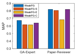
(a)

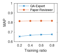
(b)

Figure 3: (a) Factor contribution analysis. WeakFG-S, WeakFG-E and WeakFG-C each stands for removing statistics, expertise matching scores, or correlations. (b) Training/test ratio analysis.

Training/Test Ratio Analysis. We further analysis on the effect of the training ratio on our WeakFG model. Figure 3(b) shows the experiment results when varying the percentage of training data. In general, we see that WeakFG’s performance stably improves by adding more training data.

Complexity and Convergence. The complexity of the proposed model is $\mathcal{O}(KNM)$, where $K$ is the number of iterations before the learning algorithm converges, $N$ is the number of nodes in the constructed factor graph, and $M$ is the number of features. The complexity is a bit higher than the comparison methods, but practically acceptable. The learning algorithm shows a very good convergent property. It takes 1,000-2,000 iterations to converge in our datasets.

4.3 Online Evaluation

Finally, we discuss the online evaluation. We developed an online reviewer recommendation system and put it into operation since early 2016. The system helps journal editors to find qualified reviewers who would accept to review manuscripts submitted to the journal. It has already been used by ten international journals.

We first evaluated its performance from a traditional expertise matching perspective. We collected 86 published papers and 2,048 candidate experts, and deployed our system to recommend reviewers to each paper. Then we asked five PhD students from the author’s lab to make relevance judgments. Basically, experts who have publication in similar topics or at least 3 papers in a related conference will be considered as relevant. Agreements of over 80% among the annotators will be taken as ground truth. In this evaluation, our system achieves comparable performance as standard expertise matching methods ($\text{P@3}=66.2\%$, where the best baseline is 69.1%). However, this evaluation did not consider whether the expert would agree to review.

We conducted another experiment to validate the system’s ability to reduce the declination rate of review invitations. The system log has recorded 2,359 review invitations for 540 papers submitted to the ten different journals until now. Figure 4(a) shows the declination rate of the ten journals. Among all the responses, 953 are “agree”, while the rest are viewed as “decline” (including “unavailable” and “no response”). Figure 4(b) shows the performance comparison between the baseline Language Model and the proposed WeakFG model. WeakFG shows clearly better performance than Language Model.

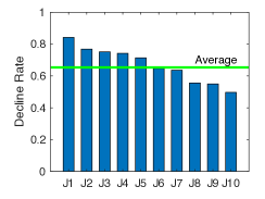
(a)

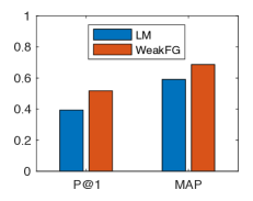
(b)

Figure 4: (a) Decline rate of paper review invitations in our data (J1-J10 represents different journals). (b) Online evaluation result of journal reviewer recommendation.

5 Conclusions

In this paper, we study an interesting problem of matching experts in online community. We propose a weakly supervised factor graph (WeakFG) model to formalize the entire problem into a principled framework. WeakFG combines expertise matching and correlations between experts using local and correlation factor functions. Our experiments on two different genres of datasets validate the effectiveness of the proposed model. We also deployed an online system to further demonstrate the advantages of the proposed model.

Acknowledgements. The work is supported by the National Basic Research Program of China (2014CB340506), the Open Project of the State Key Laboratory of Mathematical Engineering and Advanced Computing (2016A07), and the Royal Society-Newton Advanced Fellowship. Jie Tang is the corresponding author.

References

- Balog et al. [2012] Krisztian Balog, Yi Fang, Maarten de Rijke, Pavel Serdyukov, Luo Si, et al. Expertise retrieval. Foundations and Trends in Information Retrieval, 6(2–3):127–256, 2012.
- Benferhat and Lang [2001] Salem Benferhat and Jérôme Lang. Conference paper assignment. International Journal of Intelligent Systems, 16(10):1183–1192, 2001.
- Blei et al. [2003] David M Blei, Andrew Y Ng, and Michael I Jordan. Latent dirichlet allocation. Journal of Machine Learning Research, 3:993–1022, 2003.
- Buckley and Voorhees [2004] Chris Buckley and Ellen M. Voorhees. Retrieval evaluation with incomplete information. In SIGIR, 2004.
- Crandall and Huttenlocher [2006] David J Crandall and Daniel P Huttenlocher. Weakly supervised learning of part-based spatial models for visual object recognition. In ECCV, 2006.
- Deng et al. [2008] Hongbo Deng, Irwin King, and Michael R Lyu. Formal models for expert finding on dblp bibliography data. In ICDM, 2008.
- Djupe [2015] Paul A Djupe. Peer reviewing in political science: New survey results. PS: Political Science & Politics, 48(02):346–352, 2015.
- Dumais and Nielsen [1992] Susan T. Dumais and Jakob Nielsen. Automating the assignment of submitted manuscripts to reviewers. In SIGIR, 1992.
- Goldsmith and Sloan [2007] Judy Goldsmith and Robert H Sloan. The ai conference paper assignment problem. In AAAI, 2007.
- Han et al. [2016] Fangqiu Han, Shulong Tan, Huan Sun, Mudhakar Srivatsa, Deng Cai, and Xifeng Yan. Distributed representations of expertise. In SDM, 2016.
- Haym et al. [1999] Chumki Basu Haym, Haym Hirsh, William W. Cohen, and Craig Nevill-manning. Recommending papers by mining the web. In IJCAI, 1999.
- Hung et al. [2015] Nguyen Quoc Viet Hung, Duong Chi Thang, Matthias Weidlich, and Karl Aberer. Minimizing efforts in validating crowd answers. In SIGMOD, 2015.
- Ishiyama [2014] John Ishiyama. Annual report of the editors of the american political science review, 2012–2013. PS: Political Science & Politics, 47(02):542–545, 2014.
- Ishiyama [2015] John Ishiyama. Report of the editors of the american political science review, 2013–2014. PS: Political Science & Politics, 48(02):396–399, 2015.
- Joachims [2002] Thorsten Joachims. Optimizing search engines using clickthrough data. In KDD, 2002.
- Karimzadehgan and Zhai [2009] Maryam Karimzadehgan and ChengXiang Zhai. Constrained multi-aspect expertise matching for committee review assignment. In CIKM, 2009.
- Kou et al. [2015] Ngai Meng Kou, U Leong Hou, Nikos Mamoulis, and Zhiguo Gong. Weighted coverage based reviewer assignment. In SIGMOD, 2015.
- Kschischang et al. [2001] Frank R Kschischang, Brendan J Frey, and Hans-Andrea Loeliger. Factor graphs and the sum-product algorithm. IEEE Transactions on Information Theory, 47(2):498–519, 2001.
- Kusner et al. [2015] Matt J Kusner, Yu Sun, Nicholas I Kolkin, Kilian Q Weinberger, et al. From word embeddings to document distances. In ICML, 2015.
- Le and Mikolov [2014] Quoc V Le and Tomas Mikolov. Distributed representations of sentences and documents. In ICML, 2014.
- Liu et al. [2005] Xiaoyong Liu, W Bruce Croft, and Matthew Koll. Finding experts in community-based question-answering services. In CIKM, 2005.
- Long et al. [2013] Cheng Long, Raymond Chi-Wing Wong, Yu Peng, and Liangliang Ye. On good and fair paper-reviewer assignment. In ICDM, 2013.
- Mikolov et al. [2013] Tomas Mikolov, Ilya Sutskever, Kai Chen, Greg S Corrado, and Jeff Dean. Distributed representations of words and phrases and their compositionality. In NIPS, 2013.
- Mimno and McCallum [2007] David Mimno and Andrew McCallum. Expertise modeling for matching papers with reviewers. In KDD, 2007.
- Riahi et al. [2012] Fatemeh Riahi, Zainab Zolaktaf, Mahdi Shafiei, and Evangelos Milios. Finding expert users in community question answering. In WWW, 2012.
- Robertson et al. [2009] Stephen Robertson, Hugo Zaragoza, et al. The probabilistic relevance framework: Bm25 and beyond. Foundations and Trends in Information Retrieval, 3(4):333–389, 2009.
- Tajfel and Turner [2004] Henri Tajfel and John C Turner. The social identity theory of intergroup behavior. 2004.
- Tang et al. [2008] Jie Tang, Jing Zhang, Limin Yao, Juanzi Li, Li Zhang, and Zhong Su. Arnetminer: Extraction and mining of academic social networks. In KDD, 2008.
- Tang et al. [2012] Wenbin Tang, Jie Tang, Tao Lei, Chenhao Tan, Bo Gao, and Tian Li. On optimization of expertise matching with various constraints. Neurocomputing, 76(1):71–83, 2012.
- Turner and Oakes [1986] John C Turner and Penelope J Oakes. The significance of the social identity concept for social psychology with reference to individualism, interactionism and social influence. British Journal of Social Psychology, 25(3):237–252, 1986.
- Xia et al. [2017] Xin Xia, David Lo, Ying Ding, Jafar M Al-Kofahi, Tien N Nguyen, and Xinyu Wang. Improving automated bug triaging with specialized topic model. IEEE Transactions on Software Engineering, 43(3):272–297, 2017.
- Yang et al. [2009] Kai-Hsiang Yang, Tai-Liang Kuo, Hahn-Ming Lee, and Jan-Ming Ho. A reviewer recommendation system based on collaborative intelligence. In WI-IAT, 2009.
- Yedidia et al. [2000] Jonathan S Yedidia, William T Freeman, Yair Weiss, et al. Generalized belief propagation. In NIPS, 2000.
- Zhai and Lafferty [2001] Chengxiang Zhai and John Lafferty. A study of smoothing methods for language models applied to ad hoc information retrieval. In SIGIR, 2001.
- Zhang et al. [2007] Jun Zhang, Mark S. Ackerman, and Lada Adamic. Expertise networks in online communities: Structure and algorithms. In WWW, 2007.
- Zhang et al. [2008] Jing Zhang, Jie Tang, Liu Liu, and Juanzi Li. A mixture model for expert finding. In PAKDD, 2008.
- Zhao et al. [2015] Zhou Zhao, Lijun Zhang, Xiaofei He, and Wilfred Ng. Expert finding for question answering via graph regularized matrix completion. IEEE Transactions on Knowledge and Data Engineering, 27(4):993–1004, 2015.