Discontinuous polaron transition in a two-band model

Abstract

We present exact diagonalization and momentum average approximation (MA) results for the single polaron properties of a one-dimensional two-band model with phonon-modulated hopping. At strong electron-phonon coupling, we find a novel type of sharp transition, where the polaron ground state momentum jumps discontinuously from $k=\pi$ to $k=0$. The nature and origin of this transition is investigated and compared to that of the Su-Schrieffer-Heeger (SSH) model, where a sharp but smooth transition was previously reported. We argue that such discontinuous transitions are a consequence of the multi-band nature of the model, and are unlikely to be observed in one-band models. We also show that MA describes qualitatively and even quantitatively accurately this polaron and its transition. Given its computationally efficient generalization to higher dimensions, MA thus promises to allow for accurate studies of electron-phonon coupling in multi-band models in higher dimensions.

I Introduction

The coupling between carriers and phonons is known or believed to be important for many materials, including cuprates,Rösch and Gunnarsson (2004); Müller (1999); Driza et al. (2012); Gunnarsson and Rösch (2008) manganites, Müller (1999); Driza et al. (2012); Edwards (2002), nickelates Johnston et al. (2014); Müller (1999); Gou et al. (2011); Zaanen and Littlewood (1994) and bismuth perovskites.Foyevtsova et al. (2015); Franchini et al. (2009) These materials display a variety of interesting phenomena, including, but not limited to, high-temperature superconductivity (cuprates, BaBiO₃), layered ferromagnetism (manganites) and a spin/charge density wave (nickelates).

The carrier-phonon coupling leads to the formation of a polaron, a coherent quasi-particle (QP) consisting of the charge carrier and the cloud of phonons surrounding it and moving coherently with it. Polarons have been studied extensively especially in the Holstein model, Bonča et al. (1999); Ku et al. (2002); Vidmar et al. (2010); Li et al. (2010); Alvermann et al. (2010); Chandler and Marsiglio (2014); Berciu (2006); Berciu and Goodvin (2007) the simplest model where local phonons modify the on-site energy of the carrier, but also to generalizations with short-range and long-range couplings of similar origin, such as the breathing-mode (BM) model Lau et al. (2007); Pankaj and Yarlagadda (2012); Goodvin and Berciu (2008), the double-well potential modelAdolphs and Berciu (2014a, b) and the Fröhlich model Fröhlich et al. (1950); Fröhlich (1954).

The other possibility is that the coupling to phonons modulates the carrier’s hopping integrals, a scenario described by the SSH model, Su et al. (1979) which has seen an increased amount of interest in recent years.Marchand et al. (2010); Zhang et al. (2012); Herrera et al. (2013) This is because the SSH model exhibits a sharp transition in the properties of its polaron, one signature being the change of the polaron ground state (GS) momentum from $k=0$ (at weak coupling) to a finite value that smoothly evolves toward $k=\pi/2$ (at strong coupling). Such transitions were shown to be impossible for models where the phonons modulate the on-site energy Gerlach and Löwen (1991).A study of a model which includes both types of carrier-phonon coupling was carried out by Herrera et. al Herrera et al. (2013) and found that in addition to the transition observed in the SSH model, a second transition of the GS momentum also takes place. Whether other such transitions can occur and what are their characteristics, is currently an open question.

Efforts to understand polaron physics have, so far, focused almost exclusively on single-band models. It is therefore a natural question to ask whether the polaron properties of multi-band models are similar, or whether they are qualitatively different from those of single band models. In this Article, we answer this question based on a study of the single polaron properties of the two-band model depicted in Fig. 1, with two different atoms per unit cell, one of which is light and thus supports lattice vibrations (optical phonons). The coupling to this phonon mode modulates the hopping integrals, in direct analogy with the one-band SSH model.(For the vanishing carrier concentration of interest to us, the SSH-model is a one-band model because the Peierls dimerization only occurs at half-filling Marchand et al. (2010)).

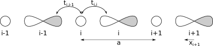
Figure 1: Sketch of the model, including the convention we use for indexing the sites and for the orientation of the lobes. The sign convention for the displacement $x_{i+1}$ due to a phonon on site $i+1$ is also shown.

Given this similarity, one may expect our two-band model to behave like the SSH model, and indeed we find a sharp transition at strong carrier-hole coupling, where the polaron GS momentum changes its value. However, unlike in the one-band SSH model where the GS momentum changes continuously with coupling, in our model the GS momentum jumps discontinuously from $k=\pi/a$ to $k=0$. Furthermore, this transition leads to an extreme flattening of the polaron band, unlike in the SSH model. We conclude that this transition is qualitatively different from that of the one-band SSH model. We argue that the mechanism for the transition is a competition between the bare carrier hopping which favors a GS momentum $k=\pi/a$, and the phonon-modulated hopping which favors $k=0$. While some of this physics is similar to that explaining the transition in the SSH model, we find strong indications that the two-band nature of our model plays a vital role. This makes it unlikely that such a discontinuous transition can occur in a one-band model. The physics described in this article is therefore, to our knowledge, fundamentally new and our findings hint at the possibility that there is still more, new polaron physics to be discovered in other multi-band models.

The physical inspiration for our model is the perovskite BaBiO₃, which is known to have strong electron-phonon coupling and to exhibit superconductivity up to surprisingly high temperatures upon hole doping ($T_{C}\sim 30K$ in the case of Ba_1-xK_xBiO₃ Cava et al. (1988) and $T_{C}\sim 13K$ for BaPb_1-xBi_xO₃) Sleight et al. (1975), widely believed to be due to a phononic glue Nourafkan et al. (2012); Yin et al. (2013); Bazhirov et al. (2013). The relevant valence orbitals are the Bi 6$s$ orbitals and the O 2$p$ orbitals.

Previous work on polarons and bipolarons in this material was carried out by Allen et al. Bischofs et al. (2002); Kostur and Allen (1997) and is based on the Rice-Sneddon model Rice and Sneddon (1981) which assumes that the Bi atoms undergo charge disproportionation, Bi⁴⁺Bi${}^{4+}\rightarrow$Bi³⁺Bi⁵⁺. This scenario has received wide-spread attention Cox and Sleight (1976, 1979); Rice and Sneddon (1981); Varma (1988); Hase and Yanagisawa (2007); Sleight (2015); Franchini et al. (2009); Bischofs et al. (2002); Kostur and Allen (1997), and as a consequence many model Hamiltonians only take into account the Bi 6$s$ orbitals. Polaronic signatures in agreement with this work have also been found experimentally Nishio et al. (2005); Derimow et al. (2014).

A different scenario is provided by a recent study of Foyevtsova et. al. Foyevtsova et al. (2015) and the experimental as well as theoretical work of Menushenkov et al Menushenkov and Klementev (2000); Menushenkov et al. (2001). Foyevtsova et. al. argue that the BiO₆ octahedra undergo a breathing distortion due to strong hybridization between the Bi 6$s$ and O 2$p$ orbitals, with the holes being located primarily on the O. This picture is similar to that proposed recently for the nickelates Mizokawa et al. (2000); Park et al. (2012); Lau and Millis (2013); Johnston et al. (2014) and the inspiration for our “toy model”. In this picture both the Bi 6$s$ and O 2$p$ orbitals need to be taken into account. Since O atoms are much lighter than Bi atoms, only optical phonons on the O atoms are considered and are allowed to modulate the hopping integrals.

When compared to other perovskites such as the cuprates, manganites and nickelates, BaBiO₃ is appealing because of its comparatively simple electronic structure and absence of magnetic properties. To simplify things even more, instead of considering a model describing such a material at or near half filling, as it is in reality, we investigate the single polaron physics in its almost fully compensated case, i.e. like in LaBiO₃ with one extra hole. Generalizing to one carrier (polaron) per unit cell will be left for future work. Moreover, as indicated above, we restrict ourselves to study a 1D BiO-like chain, instead of treating the full 3D system. There are two practical reasons for these simplifications: (i) they make comparison to the SSH model, where polaron results are currently available only for the 1D model, possible; (ii) they allow us to use exact diagonalization (ED) to find essentially exact results very efficiently,Bonča et al. (1999) which in turn also allows us to probe a wide range of coupling strengths and phonon frequencies to understand the relevant physics.

Beside using ED to understand the polaron properties of this model, we also develop and validate here two simple versions of the variational momentum average (MA) approximation,Berciu (2006); Berciu and Goodvin (2007); Goodvin and Berciu (2008) which capture the relevant polaronic physics qualitatively and even quantitatively. MA approaches are very useful because their accuracy improves in higher dimensions while maintaining similar computational efficiency. This is in contrast to ED and most other numerical methods that become very costly due to the significant increase of the Hilbert space in higher dimensions. This work can therefore be seen as a first step towards a study of the 3D systems. Note that apart from their usefulness in treating more complex problems, developing such approximations also leads to a better understanding of the nature of the polaron’s cloud.

To summarize, the research presented in this article serves two main purposes: (i) to reveal surprising, new polaron physics whose nature appears to be tied to the two-band nature of our model, and (ii) to serve as a test-ground for approximations which will be useful in solving the 3D many-band problem, and thus help to improve our understanding of the fascinating compound BaBiO₃, if the scenario of Foyevtsova et. al. turns out to be valid, or of other many-band materials with hopping-modulated carrier-phonon coupling.

The remainder of this article is organized as follows: in Sec. II we introduce the model and in Sec. III we introduce the ED algorithm, MA and a perturbation theory. The results are presented in Sec. IV and Sec. V contains our conclusions.

II Model

We study the single polaron properties of the 1D, two-band model sketched in Fig. 1. There are two atoms per unit cell, one hosting valence electrons in an $s$-orbital, and the other in a $p$-orbital. The latter atom is assumed to be sufficiently light so that it is a good approximation to ignore the motion of the heavier ones. In other words, we assume that the lighter atoms oscillate inside the “cage” made of heavier atoms, giving rise to an optical phonon mode that modulates the $s$-$p$ hopping of the carriers. We consider the limit of a very lightly doped insulator, i.e. all states are filled except for a single hole present on the chain. The inspiration to study such a model was discussed in the previous section.

The kinetic energy of the hole is described by a nearest neighbor tight-binding Hamiltonian:

$$\hat{T}_{\rm tot}=\sum_{i}(t_{i,i-1}s_{i}^{\dagger}p_{i-1}+t_{i,i}s_{i}^{\dagger}p_{i}+\text{h.c.}).$$ (1)

Here $s_{i}^{\dagger}\ (p_{i}^{\dagger})$ creates a hole on the $s$ ($p$) orbital of the atoms in the $i^{\text{th}}$ unit cell (the spin is an irrelevant degree of freedom here, and we do not write it explicitly). Their Fourier transforms are: $s_{k}^{\dagger}=\sum_{j}\exp(ikR_{j})/\sqrt{N}s_{j}^{\dagger}$ and $p_{k}^{\dagger}=\sum_{j}\exp(ikR_{j})/\sqrt{N}p_{j}^{\dagger}$, where $R_{j}=ja$ is the location of the unit cell $j=1,\dots,N$, and the number of unit cells $N\rightarrow\infty$ . The momentum $k$ is restricted to the first Brillouin zone (BZ), $-{\pi}<ka\leq{\pi}$.

For an undistorted chain (no phonons), and keeping in mind that $s_{i}^{\dagger}$ and $p_{i}^{\dagger}$ are hole operators, for the choice of lobe orientation shown in Fig. 1 we have $t_{ii}=-t_{i,i-1}=t$, leading to the kinetic energy:

$$\hat{T}=t\sum_{i}(-s_{i}^{\dagger}p_{i-1}+s_{i}^{\dagger}p_{i}+\text{h.c.})$$ (2)

The $t>0$ hopping parameter is given by the overlap of the $s$ and $p$-orbitals when the atoms are in their equilibrium positions. Changing its sign corresponds to changing the sign convention for the $p$-orbitals, and therefore does not have any physical effect. As a consequence, the results we present below for a hole-doped chain remain identical for an electron-doped chain as well. When phonons are excited, the hopping amplitudes change from this equilibrium value, resulting in the hole-phonon coupling term discussed below.

The hole’s on-site energy depends on whether it sits on an $s$- or a $p$-orbital and leads to a charge transfer term:

$$\hat{H}_{\text{ct}}=-\Delta\sum_{i}p_{i}^{\dagger}p_{i}.$$ (3)

The difference in on-site energies can have either sign, favoring the $p$ (if $\Delta>0$) or $s$ (if $\Delta<0$) orbitals. The on-site energy for the $s$ orbitals is set to zero.

The phonons are assumed to be described by a dispersionless Einstein mode with energy $\Omega$ (we set $\hbar=1$):

$$\hat{H}_{\text{ph}}=\Omega\sum_{i}b_{i}^{\dagger}b_{i},$$ (4)

where $b_{i}^{\dagger}$ creates a phonon on the $p$-orbital of the lighter atom of the $i^{\text{th}}$ unit cell. As discussed, the heavier atoms are taken to be frozen in their equilibrium positions.

This model allows for two types of hole-lattice coupling. One comes from the modulation of on-site energies, because when the distance between neighbor atoms changes, so do the corresponding Coulomb interactions. We are not aware of a comprehensive study of this type of coupling for this two-band model, although the asymptotic cases with $\Delta\rightarrow-\infty$ (the breathing-mode model Lau et al. (2007); Goodvin and Berciu (2008)) and $\Delta\rightarrow+\infty$ (the double-well modelAdolphs and Berciu (2014a, b)) have been studied and have revealed interesting polaronic behavior, although still rather conventional.

Instead, we focus here on the hole-lattice coupling arising from the fact that changes in the distance between adjacent atoms also modulate the hopping integrals. As we show below, this modulation of the kinetic energy leads to qualitatively new physics of a kind that, so far as we know, has not been revealed before.

Thus, the hole-phonon coupling that we study arises from the linear expansion of the hopping amplitudes $t_{i,i}$ and $t_{i,i-1}$ as a function of the small oxygen displacement $x_{i}\propto b_{i}+b_{i}^{\dagger}$. If we choose coordinates such that $x_{i}>0$ for a displacement toward the left, to linear order this expansion gives:

$$t_{i,i}\approx t[1+\alpha x_{i}]=t[1+\tilde{\alpha}(b_{i}+b_{i}^{\dagger})]$$ (5)

$$t_{i,i-1}\approx-t[1-\alpha x_{i-1}]=-t[1-\tilde{\alpha}(b_{i-1}+b_{i-1}^{\dagger})]$$ (6)

Within this approximation $\hat{T}_{\rm tot}=\hat{T}+\hat{H}_{\text{h-ph}}$, where after absorbing all the constants into the coupling $g$, we find:

$$\hat{H}_{\text{h-ph}}=g\sum_{i}\left[(s_{i}^{\dagger}p_{i}+s_{i+1}^{\dagger}p_{i})(b_{i}+b_{i}^{\dagger})+\text{h.c.}\right]$$ (7)

We choose $g>0$. Note that because the sign of $g$ is controlled by the choice of the coordinate system, a change $g\rightarrow-g$ is equivalent with choosing $x_{i}>0$ for displacements toward the right. Consequently the polaron properties only depend on the magnitude of $g$, not on its sign.

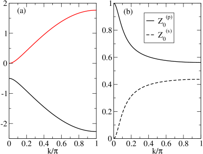
Figure 2: (color online) (a) Free hole band structure. (b) The free-hole weights $Z_{0}^{(s)}(k)$ and $Z_{0}^{(s)}(k)$ for the lower band of energy $E_{0}(k)$. In both panels $\Delta=0.5$, $t=1$ and $a=1$.

The Hamiltonian studied here is, therefore,

$$\hat{H}=\hat{T}+\hat{H}_{\text{ct}}+\hat{H}_{\text{ph}}+\hat{H}_{\text{h-ph}}.$$

Before moving on, we briefly comment on its main limitations. Keeping only linear terms in the expansion of the hopping integrals is a valid approximation when $g$ is sufficiently small, so that the polaron cloud creates rather small local distortions. For large values of $g$, the effects of higher order coupling terms $\propto(b_{i}+b_{i}^{\dagger})^{n}$ with $n>1$, need to be considered because now the local distortions become large so the displacements $x_{i}$ may no longer be assumed to be small. This is true for all models with electron-phonon coupling. For the Holstein and double-well potential models, the effect of such non-linear terms was shown to be significant in the strong coupling limit (as defined by the linear term).Adolphs and Berciu (2014a, b, 2013)

Another approximation is to consider only nearest neighbor (nn) hopping. Coming back to the inspiration for this model, for a BiO-like chain one could argue that the Bi 6$s$ orbitals are quite broad and therefore next nearest neighbor (nnn) hopping between them may play a role. Furthermore, in 3D models $t_{pp}$ hopping between nn O 2$p$ orbitals needs to be included. In 1D, however, this type of hopping is much less relevant because O atoms are separated by at least on Bi atom.

Finally, as already mentioned, hole-phonon coupling (linear or to higher order) resulting from the modulation of the on-site energies could also be included in this model. Nevertheless, here we study polaron properties for the linear model discussed above, for a wide range of $g$ values, to explore its physics and to provide a baseline from which the effect of such additional terms can be gauged. We also note that all such further extensions can be studied with the methods we use in this work.

The free-hole dispersion is obtained by diagonalizing $\hat{H}_{0}=\hat{T}+\hat{H}_{\text{ct}}$. This results in two bands with eigenenergies $-\frac{\Delta}{2}\pm\sqrt{\frac{\Delta^{2}}{4}+4t^{2}\sin^{2}{ka\over 2}}$, shown in Fig. 2(a). The lower band, which will be referred to as $E_{0}(k)$, has its minimum at $k=\pi/a$ where the hybridization between $s$ and $p$-orbitals is maximal. In contrast, the hybridization vanishes at $k=0$.

The free-hole weights $Z^{(s,p)}_{0}(k)$ are defined as

$$Z^{(s)}_{0}(k)=|\langle\Phi_{0}(k)|s_{k}^{\dagger}|0\rangle|^{2}; Z^{(p)}_{0}(k)=|\langle\Phi_{0}(k)|p_{k}^{\dagger}|0\rangle|^{2}$$ (8)

and measure the overlap between the low-energy eigenstate $|\Phi_{0}(k)\rangle$ and the free hole in a pure $s-$ or $p$-state, respectively, and are given by:

$$Z^{(s)}_{0}(k)=1-Z^{(p)}_{0}(k)=\frac{4t^{2}\sin^{2}(ka/2)}{4t^{2}\sin^{2}(ka/2)+E_{0}^{2}(k)}$$ (9)

Note that $Z^{(s)}_{0}(0)=0$ confirms that for $k=0$, the low-energy free hole sits only on the $p$-orbitals.

We are interested in the evolution of this low-energy band as the coupling to phonons is turned on, and in the nature of the resulting quasiparticle – the polaron.

III Methods

III.1 Perturbation Theory

A lot of insight can be gained from studying the anti-adiabatic limit $\Omega\gg t$, where at sufficiently small $g$ the phonon cloud of the polaron is very small, i.e. with at most one phonon present. The energy correction must be of order $g^{2}$ because $H_{\text{h-ph}}$ changes the phonon number and thus has vanishing average value in the free hole ground state.

Consider the effects of $H_{\text{h-ph}}$. For an $s$-orbital hole, it allows it to hop onto the adjacent $p$-orbital while also emitting a phonon at this $p$-orbital. The phonon needs to be reabsorbed, which can occur in two ways: (i) by hopping to the next $s$-orbital, or (ii) by hopping back to the original $s$-orbital. The first process results in an effective $s$-$s$ hopping of amplitude $-2g^{2}/\Omega\cos(ka)$, whereas the second changes the on-site $s$ energy by $-2g^{2}/\Omega$.

For a hole starting from a $p$-orbital, emission of a phonon requires the hole to hop to an adjacent $s$-orbital. From there the phonon can only be reabsorbed if the hole returns to the original $p$-orbital. This process gives an additional on-site $p$ energy of $-2g^{2}/\Omega$. Thus, the effective Hamiltonian is:

$$\hat{H}_{\text{eff}}=\left(\begin{array}[]{cc}-2t\lambda[1+\cos(ka)]&t(1-\mathrm{e}^{-ika})\\ t(1-\mathrm{e}^{ika})&-2t\lambda-\Delta\\ \end{array}\right)$$ (12)

where we introduced the dimensionless, effective coupling $\lambda=g^{2}/(\Omega t)$. The lowest eigenenergy, i.e. the polaron dispersion, is given by:

$$E_{\mathrm{P}}^{\text{eff}}(k)= -t\lambda[2+\cos(ka)]-\frac{\Delta}{2}$$

$$-\sqrt{\left[t\lambda\cos(ka)-\frac{\Delta}{2}\right]^{2}+4t^{2}\sin^{2}(\frac{ka}{2})}$$ (13)

This gives a good approximation for the polaron band in the limit $\Omega\gg t,g$, as discussed below.

III.2 Exact Diagonalization (ED)

The polaron eigenstates can also be obtained by ED. Our implementation is a direct extension of the method proposed in Ref. Bonča et al., 1999, which has already been successfully applied to a variety of polaronic models: the Holstein model in various dimensions,Bonča et al. (1999); Vidmar et al. (2010); Li et al. (2010); Ku et al. (2002); Alvermann et al. (2010) a generalized Holstein model with longer range interactions,Chandler and Marsiglio (2014) the $t$-$J$ model with hole-phonon coupling, Bonča et al. (2008) and the breathing mode model,Lau et al. (2007) to name a few. We briefly review it here.

The Hilbert space is spanned by the following translationally invariant basis states:

$$|\mathcal{C},k,\sigma\rangle=\sum_{i}\frac{\mathrm{e}^{ikR_{i}}}{\sqrt{N}}c_{i,\sigma}^{\dagger}\prod_{m\in\mathcal{C}}\frac{(b_{i+m}^{\dagger})^{n_{m}}}{\sqrt{n_{m}!}}|0\rangle$$ (14)

Here $\sigma=s,p$ is an index identifying the orbital, such that $c_{i,\text{s}}^{\dagger}=s_{i}^{\dagger}$ and $c_{i,\text{p}}^{\dagger}=p_{i}^{\dagger}$. $\mathcal{C}$ defines specific phonon cloud configurations, and $k$ is the total momentum.

Following Bonča et al., we construct the Hilbert space by acting $M$ times with the full Hamiltonian $\hat{H}$ on the free carrier states $s_{k}^{\dagger}|0\rangle$ and $p_{k}^{\dagger}|0\rangle$ and all the states which are created in this process. This quickly generates a large enough Hilbert space to accurately calculate the ground state energy of the polaron with the Lanczos technique.Dagotto (1994) Convergence is reached when an increase in the value of $M$ no longer produces a change in the eigenenergy. The number of states contained in this Hilbert subspace for different values of $M$ is listed in Table 1.

$M$	Number of states
10	4 619
11	9 227
12	18 358
13	36 314
14	71 540
15	140 943
16	276 108
17	540 923
18	1 056 244
19	2 062 913
20	4 014 953

Table 1: Number of states in the Hilbert space

III.3 Momentum average approximation (MA)

MA is an accurate variational method for calculating propagators of single polaron Hamiltonians, from which polaron properties such as its energy and quasiparticle weight can be obtained. Its simplest version was introduced for the Holstein model,Berciu (2006); Goodvin et al. (2006) and then it was shown that it can be systematically improved by increasing the size of the variational space, i.e. which phonon configurations are included.Berciu and Goodvin (2007) Apart from the Holstein model, MA has also been shown to be very accurate for many other lattice polaron models including the BM model,Goodvin and Berciu (2008) the SSH model,Marchand et al. (2010); Herrera et al. (2013) and the double-well model.Adolphs and Berciu (2014a, b)

Here we propose two versions of MA: MA⁽⁰⁾ for a variational space containing states with a one-site phonon cloud, and MA^(1r) which also includes states with one additional phonon on a site adjacent to this one-site phonon cloud. MA^(1r) is a restricted version of MA⁽¹⁾ which allows the additional phonon to be at any distance from the cloud.Berciu and Goodvin (2007) It can also be viewed as a simplified version of the two-site cloud version described in Ref. Goodvin and Berciu, 2008 for the breathing mode model. The latter can be implemented easily for this model as well but is more cumbersome to generalize to higher dimensions. As we argue below, these simpler versions already suffice for our purposes.

The Green’s functions (GF) of interest are:

$$G^{\sigma^{\prime}\sigma}(k,\omega)=\langle 0|c_{k,\sigma^{\prime}}\hat{G}(\omega)c_{k,\sigma}^{\dagger}|0\rangle,$$ (15)

where again $\sigma=s,p$ identifies the orbitals. $\hat{G}(\omega)=[\omega-\hat{H}+i\eta]^{-1}$ is the resolvent of $\hat{H}$ and $i\eta$ is a small positive imaginary number indicating that we are computing retarded GFs. A complete derivation of the MA solution can be found in Appendix A.

IV Results

We first present the ED results and discuss their meaning and implications. We then use them to gauge the accuracy of the MA⁽⁰⁾ and MA^(1r) results.

In Fig. 3 we plot the highest and lowest ED values of the polaron energy, $E_{\text{P}}(0)$ and $E_{\text{P}}(\pi)$, vs. the effective coupling $\lambda$ for two values of the phonon frequency. Results are qualitatively similar for all other tested values of $\Omega$. For small $\lambda$, the polaron GS energy (at $k=\pi$) is close to the free hole energy, $E_{\text{P}}(\pi)\approx E_{0}(\pi)=-\Delta/2-\sqrt{\Delta^{2}/4+4t^{2}}$. At $k=0$, the polaron band lies just below the polaron+phonon continuum, so $E_{\text{P}}(0)=E_{\text{P}}(\pi)+\Omega$. With increasing $\lambda$, the polaron band moves to lower energies and its bandwidth narrows considerably, as the polaron becomes heavier. All this is standard polaronic physics.

The surprise is that at sufficiently large $\lambda$, $E_{\text{P}}(0)$ and $E_{\text{P}}(\pi)$ cross, indicating that the GS momentum changes its value. For $\Omega=0.5$, in Fig. 3(a), the scale of the graph makes it difficult to see the actual crossing, but its occurrence is verified below, in Fig. 6. It is not a priori obvious that the new GS momentum is necessarily at $k=0$, but we will show below that this is the case. Consequently, we define the critical coupling $\lambda_{c}$ (or $g_{c}$) as the value for which $E_{\text{P}}(\pi)=E_{\text{P}}(0)$.

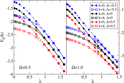
Figure 3: (color online) $E_{\text{P}}(0)$ and $E_{\text{P}}(\pi)$ vs. the effective coupling $\lambda$ for $\Omega=0.5$ (left panel), and $\Omega=1.0$ (right panel), at $\Delta=0,\pm 0.5$. Convergence was reached for $M=14,18$, respectively.

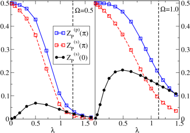
Figure 4: (color online) The QP weight $Z_{\text{P}}^{(s)}$ and $Z_{\text{P}}^{(p)}$ for $\Omega=0.5$ (left panel) and $\Omega=1.0$ (right panel). Note that $Z_{\text{P}}^{(p)}(0)=0$, because the $s$ and $p$-orbitals do not hybridize at $k=0$. The vertical, dashed line marks $\lambda_{c}$. Convergence was reached for $M=14,18$, respectively.

Changing $\Delta$ results in a shift of the polaron band. The polaron energy must be smaller than that of the free hole, and the latter is shifted downwards (upwards) for $\Delta>0$ ($\Delta<0$). A similar shift is therefore expected at least for small $\lambda$, and it is seen to appear for all $\lambda$. The effect of $\Delta$ on $\lambda_{c}$ is discussed below.

Before discussing the nature of the transition in detail, we quickly analyze the QP weight, $Z_{\text{P}}^{(s,p)}(k)$, defined as the overlap between the polaron eigenstate and the $s$ and $p$ free-hole states, respectively. They are shown in Fig. 4. Note that $Z_{\text{P}}^{(p)}(0)=0$ for any finite $\lambda$, because the $s$ and $p$ orbitals do not hybridize at $k=0$ (see Eq. (12)) and is therefore not shown. This is in stark contrast to the free hole case, where at $k=0$ all the free-hole weight is on the $p$-orbital. Consequently there is a discontinuous change in the $k=0$ QP weight when the hole-phonon coupling is turned on.

For $k=\pi$ the QP weight falls off rapidly as $\lambda$ increases, whereas for $k=0$ its projection on the $s$-orbitals first increases and then falls off more slowly. As pointed out above, this initial increase in QP weight occurs because at $k=0$ and for sufficiently small $\lambda$, the polaron band lies just below the polaron+phonon continuum.

The vertical dashed lines mark $\lambda_{c}$, the value of $\lambda$ at which the $k=\pi$ and $k=0$ polaron energies cross. Note that there is no sudden change in the QP weights at $\lambda_{c}$. This is a strong hint that the crossover is not due to a change in the nature of the phonon cloud.

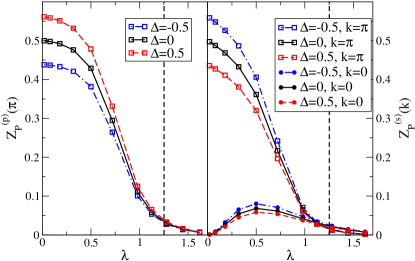
Figure 5: (color online) The QP weight $Z_{\text{P}}^{(p)}$ (left panel) and $Z_{\text{P}}^{(s)}$ (right panel) for $\Omega=0.5$. Note that $Z_{\text{P}}^{(p)}(0)=0$, because the $s$ and $p$-orbitals do not hybridize at $k=0$. The vertical, dashed line marks $\lambda_{c}$. Convergence was reached for $M=18$

The dependence of the QP weight on $\Delta$ is shown in Fig. 5 for $\Omega=0.5$. As expected, $\Delta>0$ increases the amount of $p$ character and decreases the $s$ character; $\Delta<0$ has the opposite effect. For larger values of the coupling $\lambda$, the change in QP weights due to $\Delta$ becomes negligibly small. At these values of $\lambda$ the phonon cloud is already quite sizable, as indicated by the small values of the QP weights. Together, Fig. 3 and Fig. 5 show that for strong coupling, $\Delta$ shifts the energy of the polaron but does not change the nature of its phonon cloud. This, in turn, suggests that $\hat{H}_{\text{h-ph}}$ strongly favors a specific kind of phonon cloud. In other words, there appears to be only one dominant mechanism that allows the hole to lower its energy via the emission and absorption of phonons.

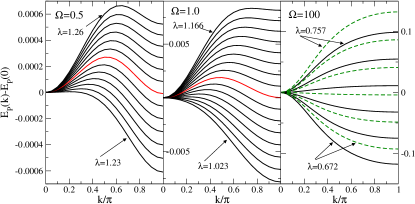
Figure 6: (color online) Polaron dispersion for $\Omega=0.5,1.0,100$ and values of $\lambda\sim\lambda_{c}$. The curves have been shifted by $E_{\text{P}}(0)$ for better comparison and the curve at $\lambda_{c}$ is highlighted in red. The green, dashed lines in the rightmost panel are the perturbative results from Eq. (13). All curves are for $\Delta=0$ and the cutoff is $M=10,14,18$, respectively.

The (shifted) polaron dispersion $E_{\text{P}}(k)-E_{\text{P}}(0)$ vs $k$, close to the critical coupling $g_{c}$, is shown in Fig. 6 for $\Omega=0.5,1.0$ and $100$. Note that close to $g_{c}$, the polaron bandwidth is extremely narrow. These results show that the GS momentum does indeed change discontinuously from $\pi$ to $0$, justifying our definition of $g_{c}$.

For $\Omega=100$, the prediction of Eq. (13) (dashed lines) agrees quite well with ED and clearly reproduces the transition. As we show now, a closer examination of this perturbative result indeed unveils a lot of the physics governing this transition. When $\lambda\ll t$, the polaron dispersion given by Eq. (13) is not much different from the free hole dispersion $E_{\text{P}}^{\text{eff}}(k)\approx E_{0}(k)$, with the ground state at $k=\pi$. For $\lambda\gg t$, on the other hand, the polaron dispersion can be approximated as:

$$E_{\text{P}}^{\text{eff}}(k)\approx-t\lambda\left[2+\cos(ka)+\left|\cos(ka)-\frac{\Delta}{2t\lambda}\right|\right]-\frac{\Delta}{2},$$ (16)

with the ground state at $k=0$ and a flat band for $ka\geq\arccos(\Delta/(2t\lambda))$. Consequently there is a critical value, $\lambda_{c}$, where the ground state momentum changes. Indeed it can be verified that for

$$\lambda_{c}=\frac{\Delta}{4t}+\sqrt{\frac{\Delta^{2}}{16t^{2}}+\frac{1}{2}},$$ (17)

the $k$-dependence in the square root of Eq. (13) exactly cancels the $-t\lambda\cos(ka)$ term and the band becomes completely flat, $E_{\text{P}}^{\text{eff}}(k)=-4t\lambda_{c}$. For $\lambda<\lambda_{c}$ the ground state is at $k=\pi$, and for $\lambda>\lambda_{c}$ it is at $k=0$.

It is clear that this change of the ground state momentum is due to a competition between the antisymmetric, bare hopping $\hat{T}$ and the symmetric, phonon-modulated hopping, $\hat{H}_{\text{h-ph}}$. To our knowledge this is the first report of a change in the ground state momentum caused by a symmetric phonon-modulated hopping; such changes have been seen before only for models with antisymmetric, phonon-modulated hopping.Zhang et al. (2012); Marchand et al. (2010) However, while for the latter case the ground-state momentum changes smoothly for $\lambda>\lambda_{c}$, here we observe a discontinuous jump from the edge to the centre of the BZ. Note, furthermore, that the hybridization between the two bands which leads to the square root in Eq. (13) plays an important role for the nature of the transition and appears to be responsible for the flatness of the band close to $\lambda_{c}$.

Although perturbation theory explains many features of the transition, there are some differences between the large $\Omega$ case and the cases where $\Omega$ is comparable to $t$. Eq. (13) predicts a completely flat band at $\lambda_{c}$. While this is seen for $\Omega=100$, it is no seen for smaller $\Omega$. Instead, here higher order processes leading to phonon-mediated, longer range effective hopping, cause the bandwidth to remain finite at all values of $\lambda$. We can attribute these processes to longer range effective hopping because they lead to a maximum at $k\approx\pi/2$, halving the BZ. Their contribution is very small, as indicated by the small bandwidth close to $\lambda_{c}$. This leads us to conclude that the phonon-assisted hopping process described in Section III.1 is indeed primarily responsible for most of the mobility of the polaron.

To make these arguments more compelling and valid for phonon clouds with more than one phonon, we now analyze the nature of the polaron cloud in more detail. For $k=0$, the polaron has QP weight on $s_{k}^{\dagger}|0\rangle$ but not $p_{k}^{\dagger}|0\rangle$. Acting with $\hat{H}_{\text{h-ph}}$ on $s_{k=0}^{\dagger}|0\rangle$ (and ignoring normalization factors) gives $\sum_{j}p_{j}^{\dagger}b_{j}^{\dagger}|0\rangle$, which we therefore expect to be a part of the polaron wavefunction. Acting on this again with $\hat{H}_{\text{h-ph}}$ gives $\sum_{j}s_{j}^{\dagger}[b_{j}^{\dagger,2}+b_{j-1}^{\dagger,2}]|0\rangle$. This pattern continues and we find that for $k=0$ the polaron eigenfunction contains states of the type $\sum_{j}p_{j}^{\dagger}b_{j}^{\dagger,2n+1}|0\rangle$, i.e. with an odd number of phonons and the hole on the same $p$-orbital, and $\sum_{j}s_{j}^{\dagger}[b_{j}^{\dagger,2n}+b_{j-1}^{\dagger,2n}]|0\rangle$, i.e. a symmetric state with an even number of phonons and the hole on the adjacent $s$-orbitals. While we only considered states with a one-site phonon cloud adjacent to the hole, this structure of the phonon cloud is indeed verified by ED, which finds very small weight for other configurations.

For $k=\pi$, $\hat{H}_{\text{h-ph}}s_{\pi}^{\dagger}|0\rangle=0$. Consequently we need to start the construction of the eigenstate from $p_{\pi}^{\dagger}|0\rangle$. Acting with $\hat{H}_{\text{h-ph}}$ gives $\sum_{j}(-1)^{j}s_{j}^{\dagger}(b_{j}^{\dagger}-b_{j-1}^{\dagger})|0\rangle$. Acting once more with $\hat{H}_{\text{h-ph}}$ gives $\sum_{j}(-1)^{j}p_{j}^{\dagger}b_{j}^{\dagger,2}|0\rangle$. This pattern generalizes and mixes states of the form $\sum_{j}(-1)^{j}p_{j}^{\dagger}b_{j}^{\dagger,2n}|0\rangle$, i.e. with an even number of phonons and the hole on the same $p$-orbital, and $\sum_{j}(-1)^{j}s_{j}^{\dagger}[b_{j}^{\dagger,2n+1}-b_{j-1}^{\dagger,2n+1}]|0\rangle$, i.e. an antisymmetric state with an odd number of phonons and the hole on the adjacent $s$-orbitals. This also is verified by ED.

Thus, the polaron cloud structure is very different at $k=0$ and $\pi$, and this has important consequences. Consider the configuration $\sum_{j}\mathrm{e}^{ikR_{j}}s_{j}^{\dagger}b_{j}^{\dagger,2n}|0\rangle$. This state can be moved by first acting $2n$ times with $\hat{H}_{\text{h-ph}}$; among other states, this links to $\sum_{j}\mathrm{e}^{ikR_{j}}s_{j+1}^{\dagger}|0\rangle$. Acting another $2n$ times with $\hat{H}_{\text{h-ph}}$ gives (among many other states) $\sum_{j}\mathrm{e}^{ikR_{j}}s_{j+1}^{\dagger}b_{j+1}^{\dagger,2n}|0\rangle$, i.e the original state translated by one site. Clearly, such processes contribute to the mobility of the polaron. Similarly, states like $\sum_{j}\mathrm{e}^{ikR_{j}}p_{j}^{\dagger}b_{j}^{\dagger,2n+1}|0\rangle$ can be moved by first acting $2n+1$ times with $\hat{H}_{\text{h-ph}}$ linking to $\sum_{j}\mathrm{e}^{ikR_{j}}s_{j+1}^{\dagger}|0\rangle$, and then to $\sum_{j}\mathrm{e}^{ikR_{j}}p_{j+1}^{\dagger}b_{j+1}^{\dagger,2n+1}|0\rangle$ after applying $\hat{H}_{\text{h-ph}}$ another $2n+1$ times. For these processes to work, it is crucial that the number of phonons is even (odd) if the carrier is on an $s(p)$ orbital. This is the case for $k=0$, but for $k=\pi$ we found that exactly the opposite is the case. This explains why the phonon-modulated effective hopping, which dominates at large couplings, favours $k=0$ and this eventually becomes the ground-state. Note, furthermore, that this discussion also illustrates why an MA version restricted to a one-site phonon cloud is expected to capture well the phenomenology of this model.

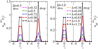
Figure 7: (color online) The phonon distribution $n_{\text{ph}}^{(\sigma)}(r_{j})$ defined in Eq. (18) for $\Omega=0.5$ (left panel) and $\Omega=1.0$ (right panel) at different values of $\lambda$. Other parameters are $k=\pi$ and $\Delta=0$. Convergence was reached for $M=14$ and $18$, respectively.

To analyze the spatial extent of the polaron cloud we calculate the phonon distribution

$$n_{\text{ph}}^{(\sigma)}(r_{j})=\sum_{i}\langle\text{P}_{\pi}|c_{i,\sigma}^{\dagger}c_{i,\sigma}b_{i+j}^{\dagger}b_{i+j}|\text{P}_{\pi}\rangle,$$ (18)

where $|\text{P}_{\pi}\rangle$ is the polaron-state with momentum $k=\pi$ and $r_{j}$ is the distance between the carrier at site $i$ and the phonon at site $i+j$. This means that $r_{j}=j$ when the carrier is on a $p$-orbital, and $r_{j}=j+1/2$ when it is on an $s$-orbital. The results are shown in Fig. 7 for $\Omega=0.5$ and $\Omega=1.0$. We see that the polaron cloud is located in the immediate vicinity of the carrier, i.e. we are dealing with a very small polaron. If the carrier is on an $s$-orbital the majority of phonons are hosted by the two oxygens next to it, while for a carrier on a $p$-orbital the three closest oxygen sites contribute. As $\lambda$ is increased past the critical coupling ($\lambda_{c}=1.25$ for $\Omega=0.5$ and $\lambda_{c}=1.13$ for $\Omega=1.0$), there is no noticeable change in the nature of the cloud. We also find that for $k=0$ and sufficiently large $\lambda$ the phonon cloud is qualitatively similar (not shown) to that for $k=\pi$. For small $\lambda$ this is not true as here the polaron state at $k=0$ is not well-separated from the polaron + phonon continuum. Reducing $\Omega$ drastically changes the overall number of phonons, but not the spatial extent of the cloud.

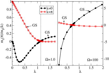
Figure 8: (color online) Inverse effective polaron mass $m_{\text{P}}^{-1}(k)$ normalized by the free hole mass $m_{0}^{-1}(\pi)$ for $\Omega=1.0$ (left panel) and $\Omega=100$ (right panel) and $\Delta=0$. The dashed line marks $\lambda_{c}$. The values of $M$ are 14 and 10, respectively.

Apart from the small bandwidth, the heavy nature of the polaron also becomes apparent from the value of its inverse effective mass, $m_{\text{P}}^{-1}(k)=\partial^{2}E_{\text{P}}/\partial k^{2}$, shown in Fig. 8 for $k=0,\pi$ at $\Omega=1.0$ and $\Omega=100$. Note that we normalize this with the free hole mass. As $\lambda\rightarrow\lambda_{c}$ from below, $m_{\text{P}}^{-1}(\pi)$ decreases indicating that the polaron becomes heavier. This is expected because as the discussion above shows, phonon-modulated hopping cannot move the polaron cloud at this momentum, and the bare hole hopping is renormalized to smaller values due to the presence of the phonon cloud. At $\lambda=\lambda_{c}$ the ground state changes momentum and consequently we now need to follow $m_{\text{P}}^{-1}(0)$ which increases because here the phonon-modulated hopping is active and increases the mobility of the polaron.

For large values of $\Omega$ the increase of $m_{\text{P}}^{-1}(0)$ for $\lambda>\lambda_{c}$ is substantial resulting in a much lighter polaron than at $\lambda<\lambda_{c}$. For smaller values of $\Omega$, on the other hand, $m_{\text{P}}^{-1}(0)$ levels off quite rapidly and the polaron remains heavy. This is to be expected because for smaller $\Omega$, the phonon cloud is quite large at $\lambda_{c}$, suppressing the polaron’s mobility. For $\Omega\gg t$, on the other hand, the average phonon number is small and an increase in $\lambda$ results in an increase of the effective hopping between $s$-orbitals. This effective hopping can become larger than the direct hopping, resulting in a lighter polaron.

A major difference between the two panels of Fig. 8 is that for $\Omega=1.0$ the inverse effective mass at $k=0$ has a minimum at finite $\lambda$. Again, this is due to the presence of the polaron+phonon continuum, which for sufficiently small $\lambda$ forces the polaron band to flatten out near $k=0$. Indeed, the location of this minimum agrees with the location of the maximum in $Z_{\text{P}}^{(s)}(0)$ in Fig. 4.

Let us now discuss the role of the charge transfer energy $\Delta$. In Fig. 9 we show the critical coupling $\lambda_{c}$ for different values of $\Delta$ and $\Omega$. The dashed lines show the perturbative result, Eq. (17), which for sufficiently large $\Omega$ is in good agreement with the ED results.

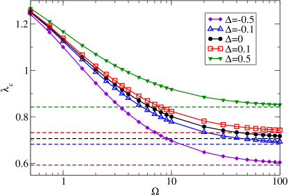
Figure 9: (color online) $\lambda_{c}$ as a function of $\Omega$ and $\Delta$. Different values of $M$ were used to ensure convergence. Dashed lines are the perturbative result from Eq. (17).

The critical coupling increases with increasing $\Delta$. This is not surprising since a large value of $\Delta$ favors the $p$ character, whereas the phonon-modulated hopping favors the $s$ character. Consequently, a negative value of $\Delta$ facilitates the transition. However, this effect is significant only for relatively large values of $\Omega$. As $\Omega$ decreases the variation of $\lambda_{c}$ with $\Delta$ becomes very small, suggesting that here $\Delta$ has little influence on the nature of the polaron cloud. This agrees with the conclusions drawn from Fig. 5. At small values of $\Omega$ the value of $\lambda_{c}$ is also much larger than that predicted by perturbation theory. However, $\lambda\propto 1/\Omega$ and in fact the transition from $k=0$ to $k=\pi$ is actually achieved at smaller values of $g$ for small $\Omega$ (see inset of Fig. 11). For these values of $\Omega$ the phonon cloud is quite large and therefore it is to be expected that the bare hopping, favoring $k=\pi$, is renormalized substantially and the phonon-modulated hopping, favoring $k=0$, wins already at smaller values of $g$.

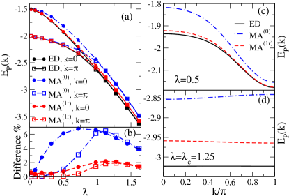
Figure 10: (color online) Comparison between ED, MA⁽⁰⁾ and MA^(1r). (a) $E_{\text{P}}(k)$ for $k=0,\ \pi$ at different values of $\lambda$. (b) The absolute value of the difference in %. (c) The dispersion $E_{\text{P}}(k)$ at $\lambda=0.5$. (d) $E_{\text{P}}(k)$ at $\lambda=\lambda_{c}=1.25$. In all cases $\Omega=0.5$ and $\Delta=0$.

This concludes our analysis of the ED results. We now briefly compare the MA predictions with the ED results, in order to validate our choice of the variational space. This is useful because MA can be much more easily and efficiently extended to higher dimensions than ED calculations. Moreover, prior workBerciu (2006); Berciu and Goodvin (2007) has shown that any version of MA becomes more accurate in higher dimensions, where the bare propagators decay faster with distance outside the free-hole continuum. Note also that MA accuracy improves with increasing phonon frequency $\Omega$;Berciu (2006); Berciu and Goodvin (2007) this is why we present results for $\Omega=0.5$ where the phonon cloud is very large at strong couplings, posing a challenging test for this (and any other) approximation.

In panel (a) of Fig. 10 we compare the MA results for the polaron energies $E_{\text{P}}(\pi),E_{\text{P}}(0)$ at different values of $\lambda$, to the ED results. As expected for a variational approach, both MA⁽⁰⁾ and MA^(1r) values are always larger than the ED ones. Panel (b) of Fig. 10 shows the relative difference between MA and ED. At small values of $\lambda$ both MA⁽⁰⁾ and MA^(1r) are very accurate, but at larger values of $\lambda$, MA^(1r) is clearly superior, showing that its additional configurations acquire finite weight. Obviously, adding more cloud configurations will further increase accuracy, but it is clear that this rather small set already suffices to capture quantitatively quite accurately the polaron properties.

A comparison for the dispersion $E_{\text{P}}(k)$ is shown in panel (c) of Fig. 10 for the intermediate coupling $\lambda=0.5$ and in panel (d) for the critical coupling $\lambda_{c}=1.25$. Panel (c) shows that both MA⁽⁰⁾ and MA^(1r) give the best results for $k=\pi$. This is probably due to the fact that at $\lambda=0.5$ the GS is still at $k=\pi$, and a variational method like MA is expected to perform best for the GS. Note that panel (b) also shows that for $\lambda<\lambda_{c}$ the relative error is smaller for $k=\pi$ than for $k=0$.

The dispersion shown in panel (d) is very narrow (on this scale). MA⁽⁰⁾ and MA^(1r) both reproduce the small bandwidth quite well, but shifted to higher energies by 2% and 6%, respectively. However, neither MA⁽⁰⁾ nor MA^(1r) predict the exact value of $\lambda_{c}=1.25$. Instead, MA⁽⁰⁾ predicts a smaller value of 1.1, whereas MA^(1r) predicts a larger value of 1.45. This trend is true for all values of $\Omega$, as shown in Fig. 11. Here we also see that MA^(1r) gives very good predictions for $\Omega>1$. The agreement becomes gradually worse as $\Omega\rightarrow 0$, where because of the low cost of phonons, the spatial extent of the phonon cloud increases beyond two sites. It also needs to be pointed out that for small values of $\Omega$ small differences in the hole-phonon coupling $g$ are amplified in the effective coupling $\lambda=g^{2}/\Omega$. For small $\Omega$ we therefore show the values of $g_{c}$ in the inset of Fig. 11.

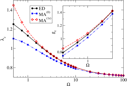
Figure 11: (color online) Comparison between the exact value of $\lambda_{c}$ obtained with ED for $\Delta=0$, and the predictions of MA⁽⁰⁾ and MA^(1r).

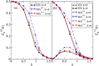
Figure 12: (color online) Comparison between ED, MA⁽⁰⁾ and MA^(1r). (a) The QP weight $Z_{\text{P}}^{(p)}(k)$ for $\pi$ for different values of $\lambda$. Note that $Z_{\text{P}}^{(p)}(0)=0$ for all $\lambda$. (b) $Z_{\text{P}}^{(p)}(k)$ for $k=0,\ \pi$. In all cases $\Omega=0.5$ and $\Delta=0$

A comparison of the QP weights obtained with MA and ED is shown in Fig. 12. Panel (a) shows $Z_{\text{P}}^{(p)}(0)$ (as pointed out above, $Z_{\text{P}}^{(p)}(\pi)=0$ for all $\lambda$). Panel (b) shows $Z_{\text{P}}^{(s)}(k)$ for $k=0$ and $k=\pi$. As expected for a variational approximation, the MA weights are larger than the ED values everywhere.

For small $\lambda$ both MA⁽⁰⁾ and MA^(1r) perform very well. The largest quantitative disagreement appears for intermediate values of $\lambda$. Here, $Z_{\text{P}}^{(s,p)}(\pi)$ falls off quite rapidly, and this is captured only qualitatively by MA. Note that MA^(1r) performs much better than MA⁽⁰⁾ in this $\lambda$-range, indicating that a further improvement of MA by adding phonons on adjacent sites is possible. The results improve substantially for $\lambda>\lambda_{c}$. At these values, the QP weight does not change as rapidly anymore. We find that here MA⁽⁰⁾ and MA^(1r) are on equal footing, with MA⁽⁰⁾ actually outperforming MA^(1r) at $\lambda=1.45$. This could be related to the fact that MA^(1r) predicts a value that is too large for $\lambda_{c}$, whereas MA⁽⁰⁾ predicts a value that is smaller than the exact result.

V Conclusions

We have investigated the effect of phonon-modulated hopping in a two-band model describing a chain with alternating atoms with $s$ and $p$ valence orbitals, respectively. As discussed in the Introduction, part of the motivation for this work is to study a toy 1D model inspired by the perovskite LaBiO₃ (or nearly fully compensated BaBiO₃) in the scenario where holes are primarily located on the O atoms, to understand the properties of the resulting polaron and to develop a good approximation that can be easily generalized for similar 3D system.

The key finding is that at sufficiently large hole-phonon coupling, the polaron undergoes a sharp transition where its GS momentum jumps from $\pi$ to $0$. Sharp polaron transitions have been observed previously in the SSH and related models with phonon-modulated hopping, Marchand et al. (2010); Zhang et al. (2012); Herrera et al. (2013) however there are qualitative differences between our results and those of these studies. In these other models the momentum changes smoothly as the effective coupling is increased. Also, the polaron mass diverges at the transition but remains finite (and can be surprisingly light) in the limit of infinite effective coupling. In our model, on the other hand, there is a discontinuous jump of the momentum from $k=\pi$ to $k=0$. To the best of our knowledge, such a discontinuous transition has not been discussed before. These results suggest that there may be more new physics to be discovered in models of carrier-phonon coupling different from that of the much studied one-band models of the Holstein and Fröhlich type.

We argued that this transition is due to a competition between the bare hopping $\hat{T}$ and the phonon-modulated hopping $\hat{H}_{\text{h-ph}}$: the former favors a $k=\pi$ ground state, while the latter increases polaron mobility at $k=0$ but not at $k=\pi$. This analysis suggests that a transition can only occur when $\hat{T}$ and $\hat{H}_{\text{h-ph}}$ have different symmetries. This is supported by the findings of Zhang et. al. Zhang et al. (2012) who report a transition in an SSH-like model for symmetric bare hopping and antisymmetric phonon-modulated hopping, but not for symmetric phonon-modulated hopping.

We have used arguments based on perturbation theory, but also more general symmetry arguments, to support the view that the discontinuous nature of this transition is closely tied to the two-band nature of the model. In perturbation theory the hybridization between the $s$ and $p$ bands leads to the square root dependence in Eq. (13), which is the main ingredient needed for this type of discontinuous jump of the GS momentum. We believe that it is highly unlikely that a transition with such a discontinuous jump can be found in a one-band model. This suggests that the polaron properties of multi-band models are qualitatively different from those of one-band models, and that more work needs to be done to exhaustively study all possible types of polaron transitions. Whether such transitions also occurs in 2D and 3D models where nn hopping between oxygens is also included is not a priori clear; we believe this to be the case and we are currently investigating such models.

When extended to one-site phonon cloud configurations with an arbitrary number of phonons, the arguments mentioned above allowed us to elucidate the mechanism behind the transition. They also suggested two types of MA variational approximations, where the phonon cloud is restricted to be one-site in extent (MA⁽⁰⁾) and one-site cloud with at most one additional phonon on an adjacent site (MA^(1r)). We find that MA⁽⁰⁾ reproduces the GS energy with an accuracy of 6% or better while MA^(1r) yields even better results with an accuracy of at least 2%. These values were found for $\Omega=0.5$ where the phonon cloud is already very large, and therefore show that MA performs well even under difficult conditions.

Of course, the MA accuracy is significantly less for the QP weights at intermediate coupling $\lambda$. This is not surprising, because the part of the eigenstates ignored by the variational calculation does contribute to the wavefunctions’ normalization (and therefore serves to lower the QP weight) even if it may not have much effect on the eigenenergy. It is important to note, however, that both MA approaches reproduce the qualitative behavior correctly, and that adding more variational states will further improve quantitative agreement. MA is also successful in predicting an accurate value for the critical coupling $\lambda_{c}$ for not too small phonon frequencies. At small $\Omega$, $\lambda_{c}$ is underestimated by MA⁽⁰⁾ and overestimated by MA^(1r), so at least they provide bounds for its true value.

The major advantage of MA, when compared to ED, is its numerical cost. For MA⁽⁰⁾ one merely needs to multiply $2\times 2$-matrices, whereas for MA^(1r) the largest matrix size is $17\times 17$. In fact one can also store all of the $\alpha_{n}$ and $\beta_{n}$ in one large sparse matrix, which further increases performance. The essential aspect is that in both cases the number of states for a given number $n$ of phonons is independent of $n$. This is why generalizing these MA approaches to 3D will be significantly more efficient than for more general MA schemes, like that of Ref. Goodvin and Berciu, 2008. We have shown that in 1D these schemes already work quite well, and since MA improves its accuracy in higher dimension, these generalizations should suffice to accurately and efficiently obtain polaron properties in the multi-band, 3D model. This work is now in progress.

Appendix A MA equations of motion

The equations of motion (eom) for $G^{\sigma^{\prime}\sigma}(k,\omega)$ can be constructed by repeatedly using Dyson’s identity $\hat{G}(\omega)=\hat{G}_{0}(\omega)+\hat{G}(\omega)\hat{V}\hat{G}_{0}(\omega)$, where $\hat{H}=\hat{H}_{0}+\hat{V}$ and $\hat{G}_{0}(\omega)$ is the resolvent for $\hat{H}_{0}$. Choosing $\hat{V}=\hat{H}_{\text{h-ph}}$ and doing this once yields:

$$G^{\sigma^{\prime}\sigma}(k,\omega)= G_{0}^{\sigma^{\prime}\sigma}(k,\omega)+g\left(1+\mathrm{e}^{ika}\right)f_{p,0}^{(1)}(k,\omega)G_{0}^{s\sigma}(k,\omega)$$

$$+\left(f_{s,0}^{(1)}(k,\omega)+f_{s,1}^{(1)}\right)G_{0}^{p\sigma}(k,\omega),$$ (19)

where we defined the generalized GFs:

$$f_{\sigma,l}^{(n)}(k,\omega)=\sum_{j}\frac{\mathrm{e}^{ikR_{j}}}{\sqrt{N}}\langle 0|c_{k,\sigma^{\prime}}\hat{G}(\omega)c_{j+l,\sigma}^{\dagger}(b_{j}^{\dagger})^{n}|0\rangle.$$ (20)

These describe the projection onto states with a one-site phonon cloud, and are therefore the only GFs included in MA⁽⁰⁾. Note that we suppressed the $\sigma^{\prime}$ index in the definition of the generalized GFs since the eom do not couple to GFs with different $\sigma^{\prime}$. For MA^(1r), we also include the contribution from the generalized GFs:

$$F_{\sigma,l}^{(1,n)}(k,\omega)=\sum_{j}\frac{\mathrm{e}^{ikR_{j}}}{\sqrt{N}}\langle 0|c_{k,\sigma^{\prime}}\hat{G}(\omega)c_{j+l,\sigma}^{\dagger}b_{j-1}^{\dagger}(b_{j}^{\dagger})^{n}|0\rangle$$

$$F_{\sigma,l}^{(n,1)}(k,\omega)=\sum_{j}\frac{\mathrm{e}^{ikR_{j+1}}}{\sqrt{N}}\langle 0|c_{k,\sigma^{\prime}}\hat{G}(\omega)c_{j+l,\sigma}^{\dagger}(b_{j}^{\dagger})^{n}b_{j+1}^{\dagger}|0\rangle$$

with one additional phonon either to the left or to the right of the phonon cloud. Note that for $n=1$, $F_{\sigma,l}^{(1,n)}(k,\omega)=F_{\sigma,l}^{(n,1)}(k,\omega)$.

We now apply Dyson’s identity again, to obtain the eom for the generalized GFs. Suppressing the $(k,\omega)$ argument for simplicity, we find:

$$f_{\sigma,l}^{(n)} =(nf_{s,0}^{(n-1)}+f_{s,0}^{(n+1)}+nf_{s,1}^{(n-1)}+f_{s,1}^{(n+1)})\bar{g}_{-l}^{p,\sigma}$$

$$+(F_{s,-1}^{(1,n)}+F_{s,0}^{(1,n)})\bar{g}_{-l-1}^{p,\sigma}+\mathrm{e}^{-ika}(F_{s,1}^{(n,1)}+F_{s,2}^{(n,1)})$$

$$\times\bar{g}_{-l+1}^{p,\sigma}+(nf_{p,0}^{(n-1)}+f_{p,0}^{(n+1)})(\bar{g}_{-l}^{s,\sigma}+\bar{g}_{-l+1}^{s,\sigma})$$

$$+F_{p,-1}^{(1,n)}(\bar{g}_{-l-1}^{s,\sigma}+\bar{g}_{-l}^{s,\sigma})+\mathrm{e}^{-ika}F_{p,1}^{(n,1)}.$$

$$\times(\bar{g}_{-l+1}^{s,\sigma}+\bar{g}_{-l+2}^{s,\sigma})$$ (21)

$$F_{\sigma,l}^{(1,n)} =(nF_{s,0}^{(1,n-1)}+F_{s,0}^{(1,n+1)}+nF_{s,1}^{(1,n-1)}+F_{s,1}^{(1,n+1)})\bar{g}_{-l}^{p,\sigma}$$

$$+(f_{s,-1}^{(n)}+f_{s,0}^{(n)})\bar{g}_{-l-1}^{p,\sigma}+(nF_{p,0}^{(1,n-1)}+F_{p,0}^{(1,n+1)})$$

$$\times(\bar{g}_{-l}^{s,\sigma}+\bar{g}_{-l+1}^{s,\sigma})+f_{p,-1}^{(n)}(\bar{g}_{-l-1}^{s,\sigma}+\bar{g}_{-l}^{s,\sigma}).$$ (22)

$$F_{\sigma,l}^{(n,1)} =(nF_{s,0}^{(n-1,1)}F_{s,0}^{(n+1,1)}+nF_{s,1}^{(n-1,1)}+F_{s,1}^{(n+1,1)})\bar{g}_{-l}^{p,\sigma}$$

$$+(\mathrm{e}^{ika}f_{s,1}^{(n)}+\mathrm{e}^{ika}f_{s,2}^{(n)})\bar{g}_{-l+1}^{p,\sigma}$$

$$+(nF_{p,0}^{(n-1,1)}+F_{p,0}^{(n+1,1)})(\bar{g}_{-l}^{s,\sigma}+\bar{g}_{-l+1}^{s,\sigma})$$

$$+\mathrm{e}^{ika}f_{p,1}^{(n)}(\bar{g}_{-l+1}^{s,\sigma}+\bar{g}_{-l+2}^{s,\sigma}),$$ (23)

where we introduced the free hole real-space GFs:

$$\bar{g}_{l}^{\sigma^{\prime},\sigma}\equiv\bar{g}_{l}^{\sigma^{\prime},\sigma}(\omega-n\Omega)={g\over N}\sum_{q}\mathrm{e}^{iqR_{l}}G_{0}^{\sigma^{\prime}\sigma}(q,\omega-n\Omega).$$

For simplicity its $(\omega-n\Omega)$ argument was again suppressed in the equations above. In 1D, these free hole real-space GFs can be obtained analytically, see Appendix B.

The right hand side of these eom only links to generalized GFs with specific values of $l$. Let us first consider the case of MA⁽⁰⁾. Here we only consider generalized GFs of the type $f_{\sigma,l}^{(n)}$. By inspection of Eq. (21) we find that the eom only link to $\tilde{f}_{s}^{(n)}=f_{s,0}^{(n)}+f_{s,1}^{(n)}$ and $\tilde{f}_{p}^{(n)}=f_{p,0}^{(n)}$. Furthermore since $\bar{g}_{0}^{p,s}+\bar{g}_{-1}^{p,s}=0$ and $g_{0}^{s,p}+g_{1}^{s,p}=0$ and $\bar{g}_{-l}^{\sigma,\sigma}=\bar{g}_{l}^{\sigma,\sigma}$ (see Appendix B) the eom simplify to:

$$\tilde{f}_{s}^{(n)}=2(\bar{g}_{0}^{s,s}+\bar{g}_{1}^{s,s})(n\tilde{f}_{p}^{(n-1)}+\tilde{f}_{p}^{(n+1)})$$ (24)

$$\tilde{f}_{p}^{(n)}=\bar{g}_{0}^{p,p}(n\tilde{f}_{s}^{(n-1)}+\tilde{f}_{s}^{(n+1)}).$$ (25)

We define the column vector $\mathbf{\tilde{v}}_{n}=(\tilde{f}_{s}^{(n)},\tilde{f}_{p}^{(n)})^{T}$ and recast the eom in the form

$$\mathbf{\tilde{v}}_{n}=\alpha_{n}\mathbf{\tilde{v}}_{n-1}+\beta_{n}\mathbf{\tilde{v}}_{n+1},$$ (26)

where $\tilde{\alpha}_{n}$ and $\tilde{\beta}_{n}$ are $2\times 2$-matrices which for $n\geq 2$ can be read off directly from the equations above. To get $\tilde{\alpha}_{1}$ we use $\tilde{f}_{s}^{(0)}=(1+\mathrm{e}^{-ika})G^{\sigma^{\prime}s}$ and $\tilde{f}_{p}^{(0)}=G^{\sigma^{\prime}p}$, where $\sigma^{\prime}$ is the same as in Eq. (19). The eom can now be solved with the ansatz $\mathbf{\tilde{v}}_{n}=\tilde{A}_{n}\mathbf{\tilde{v}}_{n-1}$, Goodvin and Berciu (2008) which is justified because for large $n$, $\bar{g}_{l}^{\sigma^{\prime},\sigma}(\omega-n\Omega)$ goes to zero and therefore $\mathbf{\tilde{v}}_{n}$ must go to zero as well. Plugging this ansatz back into Eq. (35) yields $\tilde{A}_{n}=[1-\tilde{\beta}_{n}\tilde{A}_{n+1}]^{-1}\tilde{\alpha}_{n}$ which can be calculated recursively starting with $\tilde{A}_{M_{c}+1}=0$, where $M_{c}$ is chosen sufficiently large so that its further increase has no effect on the results.

Once we have calculated $\tilde{A}_{1}$ linking $\mathbf{\tilde{v}}_{1}$ to $\mathbf{\tilde{v}}_{0}^{\sigma^{\prime}}=(G^{\sigma^{\prime}s},G^{\sigma^{\prime}p})^{T}$, we can rewrite Eq. (19) in matrix form:

$$G(k,\omega)=G_{0}(k,\omega)+gG(k,\omega)\tilde{A}_{1}^{T}\tilde{M}G_{0}(k,\omega),$$ (27)

Note that this requires identifying the first row of $G(k,\omega)$ with $(\mathbf{v}_{0}^{s})^{T}$ and the second row with $(\mathbf{v}_{0}^{p})^{T}$. $\tilde{M}$ is the $2\times 2$-matrix with $\tilde{M}_{1,1}=\tilde{M}_{2,2}=0,\tilde{M}_{1,2}=1,\tilde{M}_{2,1}=1+\mathrm{e}^{ika}$. The self-energy $\Sigma(k,\omega)$ is defined by the $2\times 2$-matrix equation $G(k,\omega)=[G_{0}(k,\omega)-\Sigma(k,\omega)]^{-1}$. In the MA⁽⁰⁾ approximation it is therefore given by:

$${\Sigma}_{(0)}(k,\omega)=g\tilde{A}_{1}^{T}\tilde{M}.$$ (28)

We now show how to use the MA⁽⁰⁾ eom to rigorously derive the perturbation result of Sec. III.1. For a cutoff of $M_{c}=1$, we find that

$$\tilde{A}_{1}=\tilde{\alpha_{1}}=\left(\begin{array}[]{cc}0&2(\bar{g}_{0}^{s,s}+\bar{g}_{1}^{s,s})\\ \bar{g}_{0}^{p,p}(1+\mathrm{e}^{-ika})&0\\ \end{array}\right)$$ (31)

and consequently

$$\tilde{\Sigma}^{(M_{c}=1)}=2g\left(\begin{array}[]{cc}(1+\cos(ka))\bar{g}_{0}^{p,p}&0\\ 0&\bar{g}_{0}^{s,s}+\bar{g}_{1}^{s,s}\\ \end{array}\right)$$ (34)

For $\Omega\gg t,\Delta$ we have $\bar{g}_{0}^{s,s}\approx\bar{g}_{0}^{p,p}\approx-g/\Omega$ and $\bar{g}_{1}^{s,s}\approx 0$ (see Appendix B) and we recover the result of Eq. (12).

The MA^(1r) case is treated in exactly the same manner, but is slightly more tedious. For $n>2$ phonons we include the following 17 GFs: $f_{s,l}^{(n)}$ with $l\in\{-1,0,1,2\}$; $f_{p,l}^{(n)}$ with $l\in\{-1,0,1\}$; $F_{s,l}^{(1,n-1)}$ with $l\in\{-1,0,1\}$; $F_{p,l}^{(1,n-1)}$ with $l\in\{-1,0\}$; $F_{s,l}^{(n-1,1)}$ with $l\in\{0,1,2\}$; and $F_{p,l}^{(n-1,1)}$ with $l\in\{0,1\}$. For $n=2$, some of these GFs are identical so that their number is reduced to 12. Similarly, for $n=1$ one only needs to keep 7 GFs.

The generalized GFs are again arranged in a vector $\mathbf{v}_{n}$ and the eom recast as a recurrence equation:

$$\mathbf{v}_{n}=\alpha_{n}\mathbf{v}_{n-1}+\beta_{n}\mathbf{v}_{n+1}.$$ (35)

The matrices $\alpha_{n}$ and $\beta_{n}$ can be read off from Eqs. (21), (22) and (23). Furthermore, Eq. (20) indicates that $(f_{s,0}^{(0)},f_{s,1}^{(0)},f_{p,0}^{0})=(G^{\sigma^{\prime}s},\mathrm{e}^{-ika}G^{\sigma^{\prime}s},G^{\sigma^{\prime}p})$ which we use to read off $\alpha_{1}$. Again the eom are solved with the ansatz $\mathbf{v}_{n}=A_{n}\mathbf{v}_{n-1}$ Goodvin and Berciu (2008), yielding $A_{n}=[1-\beta_{n}A_{n+1}]^{-1}\alpha_{n}$.

We then rewrite Eq. (19) in matrix form:

$$G(k,\omega)=G_{0}(k,\omega)+gG(k,\omega)A_{1,r}^{T}MG_{0}(k,\omega),$$ (36)

Here $A_{1,r}$ is a reduced version of $A_{1}$. It is a $3\times 2$-matrix which only contains the rows of $A_{1}$ linking $f_{s,0}^{(1)},f_{s,1}^{(1)}$ and $f_{p,0}^{(1)}$ to $\mathbf{v}_{0}$. This is necessary since the other 4 generalized GFs contained in $\mathbf{v}_{1}$ do not appear in Eq. (19). The matrix $M$ is a $3\times 2$-matrix whose only non-zero elements are $M_{3,1}=1+\mathrm{e}^{ika}$ and $M_{1,2}=M_{2,2}=1$. The self-energy $\Sigma(k,\omega)$ in the MA^(1r) approximation is, then:

$$\Sigma_{(1r)}(k,\omega)=g\tilde{A}_{1,r}^{T}M.$$ (37)

Appendix B Real-Space Green’s functions (GFs)

The real-space GFs of $\hat{H}_{0}=\hat{T}+\hat{H}_{\text{ct}}+\hat{H}_{\text{ph}}$ are defined as $g_{0}^{\sigma^{\prime},\sigma}(R_{l},\omega)=\sum_{q}\frac{\mathrm{e}^{iqR_{j+l}}}{\sqrt{N}}G_{0}(q,\omega)$. This can be rewritten as $g_{0}^{\sigma^{\prime},\sigma}(R_{l},\omega)=\langle 0|c_{\sigma^{\prime},l}\hat{G}(\omega)c_{\sigma,0}|0\rangle$, i.e. $g_{0}^{\sigma^{\prime},\sigma}(R_{l},\omega)$ measures the probability amplitude that a hole injected at site 0 will be removed at site $l$. The eom are obtained using Dyson’s identity. For $\sigma^{\prime}=p$, and suppressing the $(k,\omega)$-dependence, we find:

$$g_{0}^{p,p}(\tilde{\omega}+\Delta)=1-tg_{-1}^{p,s}+tg_{0}^{p,s}$$ (38)

$$g_{-1}^{p,s}\tilde{\omega}=-tg_{0}^{p,p}+tg_{-1}^{p,p}$$ (39)

$$g_{0}^{p,s}\tilde{\omega}=-tg_{1}^{p,p}+tg_{0}^{p,p},$$ (40)

where we defined the shorthand $\tilde{\omega}=\omega+i\eta$. For $n\neq 0,-1$, the general form of the eom is

$$g_{n}^{p,p}(\tilde{\omega}+\Delta)=-tg_{n-1}^{p,s}+tg_{n}^{p,s}$$ (41)

$$g_{n}^{p,s}\tilde{\omega}=-tg_{n+1}^{p,p}+tg_{1}^{p,p}$$ (42)

Eliminating $g_{n}^{p,s}$, the eom for $g_{n}^{p,p}$, with $n\neq 0,-1$, can be recast as

$$g_{n}^{p,p}[\tilde{\omega}(\tilde{\omega}+\Delta)-2t^{2}]=-t^{2}g_{n-1}^{p,p}-t^{2}g_{n+1}^{p,p}$$ (43)

Similarly we find

$$g_{0}^{p,p}(\tilde{\omega}(\tilde{\omega}+\Delta)-2t^{2})=\tilde{\omega}-t^{2}(g_{-1}^{p,p}+g_{1}^{p,p})$$ (44)

In the time-domain the small imaginary part $i\eta$ corresponds to a finite lifetime of the hole. Therefore the probability that a hole travels from site 0 to site $j$ falls off exponentially as $\eta j$. and we use the ansatz $g_{n}^{p,p}=zg_{n-1}^{p,p}$, for $n>0$. For $n<-1$ we need to use $g_{n}^{p,p}=zg_{n+1}^{p,p}$. In both cases, plugging the ansatz back into the eom gives:

$$z_{\pm}=-\left(\frac{\tilde{\omega}(\tilde{\omega}+\Delta)}{2t^{2}}-1\right)\pm\sqrt{\left(\frac{\tilde{\omega}(\tilde{\omega}+\Delta)}{2t^{2}}-1\right)^{2}-1},$$ (45)

We need to choose the solution which satisfies $|z|<1$. Using the ansatz in Eq. (44) we obtain

$$g_{0}^{p,p}=\frac{\tilde{\omega}}{\tilde{\omega}(\tilde{\omega}+\Delta)+2t^{2}(z-1)}$$ (46)

From this all the other $g_{n}^{p,p}$ are obtained as $g_{n}^{p,p}=z^{|n|}g_{0}^{p,p}$.

We can apply the same procedure to find analytical expressions for the $g_{n}^{p,s}$. However, we need to be careful since both $g_{-1}^{p,s}$ and $g_{0}^{p,s}$ link to $g_{0}^{pp}$ and therefore need to be treated separately. After some algebra we find

$$g_{0}^{p,s}=-g_{-1}^{p,s}=\frac{t}{\tilde{\omega}(\tilde{\omega}+\Delta)+t^{2}(z-3)}$$ (47)

$$g_{n}^{p,s}=z^{n}g_{0}^{p,s}, n>0$$ (48)

$$g_{n}^{p,s}=z^{|n|-1}g_{-1}^{p,s}, n<-1$$ (49)

Similarly one finds:

$$g_{0}^{s,s}=\frac{\tilde{\omega}+\Delta}{\tilde{\omega}(\tilde{\omega}+\Delta)+2t^{2}(z-1)}$$ (50)

$$g_{n}^{s,s}=z^{|n|}g_{0}^{s,s}$$ (51)

$$g_{0}^{s,p}=-g_{1}^{s,p}=\frac{t}{\tilde{\omega}(\tilde{\omega}+\Delta)+t^{2}(z-3)}$$ (52)

$$g_{n}^{p,s}=z^{|n|}g_{0}^{p,s}, n<0$$ (53)

$$g_{n}^{p,s}=z^{n-1}g_{1}^{p,s}, n>1$$ (54)

Note that for $|\omega|\gg t,\Delta$, Eq. (45) implies that $z\rightarrow 0$. Using this in the expressions for $g_{0,-1}^{p,s}(\omega)$ and $g_{0,1}^{s,p}(\omega)$ we find that they scale as $\pm 1/\omega^{2}$. The diagonal real-space GFs, $g_{0}^{s,s}$ and $g_{0}^{p,p}$ on the other hand scale as $1/\omega$. All real-space GFs with larger values of $|n|$ go to 0 since $z\rightarrow 0$.

References

- Rösch and Gunnarsson (2004) O. Rösch and O. Gunnarsson, Phys. Rev. Lett. 92, 146403 (2004).
- Müller (1999) K. Müller, Journal of Superconductivity 12, 3 (1999).
- Driza et al. (2012) N. Driza, S. Blanco-Canosa, M. Bakr, S. Soltan, M. Khalid, L. Mustafa, K. Kawashima, G. Christiani, H.-U. Habermeier, G. Khaliullin, C. Ulrich, M. Le Tacon, and B. Keimer, Nat Mater 11, 675 (2012).
- Gunnarsson and Rösch (2008) O. Gunnarsson and O. Rösch, Journal of Physics: Condensed Matter 20, 043201 (2008).
- Edwards (2002) D. M. Edwards, Advances in Physics 51, 1259 (2002).
- Johnston et al. (2014) S. Johnston, A. Mukherjee, I. Elfimov, M. Berciu, and G. A. Sawatzky, Phys. Rev. Lett. 112, 106404 (2014).
- Gou et al. (2011) G. Gou, I. Grinberg, A. M. Rappe, and J. M. Rondinelli, Phys. Rev. B 84, 144101 (2011).
- Zaanen and Littlewood (1994) J. Zaanen and P. B. Littlewood, Phys. Rev. B 50, 7222 (1994).
- Foyevtsova et al. (2015) K. Foyevtsova, A. Khazraie, I. Elfimov, and G. A. Sawatzky, Phys. Rev. B 91, 121114 (2015).
- Franchini et al. (2009) C. Franchini, G. Kresse, and R. Podloucky, Phys. Rev. Lett. 102, 256402 (2009).
- Bonča et al. (1999) J. Bonča, S. A. Trugman, and I. Batistić, Phys. Rev. B 60, 1633 (1999).
- Ku et al. (2002) L.-C. Ku, S. A. Trugman, and J. Bonča, Phys. Rev. B 65, 174306 (2002).
- Vidmar et al. (2010) L. Vidmar, J. Bonča, and S. A. Trugman, Phys. Rev. B 82, 104304 (2010).
- Li et al. (2010) Z. Li, D. Baillie, C. Blois, and F. Marsiglio, Phys. Rev. B 81, 115114 (2010).
- Alvermann et al. (2010) A. Alvermann, H. Fehske, and S. A. Trugman, Phys. Rev. B 81, 165113 (2010).
- Chandler and Marsiglio (2014) C. J. Chandler and F. Marsiglio, Phys. Rev. B 90, 125131 (2014).
- Berciu (2006) M. Berciu, Phys. Rev. Lett. 97, 036402 (2006).
- Berciu and Goodvin (2007) M. Berciu and G. L. Goodvin, Phys. Rev. B 76, 165109 (2007).
- Lau et al. (2007) B. Lau, M. Berciu, and G. A. Sawatzky, Phys. Rev. B 76, 174305 (2007).
- Pankaj and Yarlagadda (2012) R. Pankaj and S. Yarlagadda, Phys. Rev. B 86, 035453 (2012).
- Goodvin and Berciu (2008) G. L. Goodvin and M. Berciu, Phys. Rev. B 78, 235120 (2008).
- Adolphs and Berciu (2014a) C. P. J. Adolphs and M. Berciu, Phys. Rev. B 89, 035122 (2014a).
- Adolphs and Berciu (2014b) C. P. J. Adolphs and M. Berciu, Phys. Rev. B 90, 085149 (2014b).
- Fröhlich et al. (1950) H. Fröhlich, H. Pelzer, and S. Zienau, The London, Edinburgh, and Dublin Philosophical Magazine and Journal of Science 41, 221 (1950).
- Fröhlich (1954) H. Fröhlich, Advances in Physics 3, 325 (1954).
- Su et al. (1979) W. P. Su, J. R. Schrieffer, and A. J. Heeger, Phys. Rev. Lett. 42, 1698 (1979).
- Marchand et al. (2010) D. J. J. Marchand, G. De Filippis, V. Cataudella, M. Berciu, N. Nagaosa, N. V. Prokof’ev, A. S. Mishchenko, and P. C. E. Stamp, Phys. Rev. Lett. 105, 266605 (2010).
- Zhang et al. (2012) Y. Zhang, L. Duan, Q. Chen, and Y. Zhao, The Journal of Chemical Physics 137, 034108 (2012).
- Herrera et al. (2013) F. Herrera, K. W. Madison, R. V. Krems, and M. Berciu, Phys. Rev. Lett. 110, 223002 (2013).
- Gerlach and Löwen (1991) B. Gerlach and H. Löwen, Rev. Mod. Phys. 63, 63 (1991).
- Cava et al. (1988) R. J. Cava, B. Batlogg, J. J. Krajewski, R. Farrow, L. W. Rupp, A. E. White, K. Short, W. F. Peck, and T. Kometani, Nature 332, 814 (1988).
- Sleight et al. (1975) A. Sleight, J. Gillson, and P. Bierstedt, Solid State Communications 17, 27 (1975).
- Nourafkan et al. (2012) R. Nourafkan, F. Marsiglio, and G. Kotliar, Phys. Rev. Lett. 109, 017001 (2012).
- Yin et al. (2013) Z. P. Yin, A. Kutepov, and G. Kotliar, Phys. Rev. X 3, 021011 (2013).
- Bazhirov et al. (2013) T. Bazhirov, S. Coh, S. G. Louie, and M. L. Cohen, Phys. Rev. B 88, 224509 (2013).
- Bischofs et al. (2002) I. B. Bischofs, V. N. Kostur, and P. B. Allen, Phys. Rev. B 65, 115112 (2002).
- Kostur and Allen (1997) V. N. Kostur and P. B. Allen, Phys. Rev. B 56, 3105 (1997).
- Rice and Sneddon (1981) T. M. Rice and L. Sneddon, Phys. Rev. Lett. 47, 689 (1981).
- Cox and Sleight (1976) D. Cox and A. Sleight, Solid State Communications 19, 969 (1976).
- Cox and Sleight (1979) D. E. Cox and A. W. Sleight, Acta Crystallographica Section B 35, 1 (1979).
- Varma (1988) C. M. Varma, Phys. Rev. Lett. 61, 2713 (1988).
- Hase and Yanagisawa (2007) I. Hase and T. Yanagisawa, Phys. Rev. B 76, 174103 (2007).
- Sleight (2015) A. W. Sleight, Physica C: Superconductivity and its Applications 514, 152 (2015), superconducting Materials: Conventional, Unconventional and Undetermined.
- Nishio et al. (2005) T. Nishio, J. Ahmad, and H. Uwe, Phys. Rev. Lett. 95, 176403 (2005).
- Derimow et al. (2014) N. Derimow, J. Labry, A. Khodagulyan, J. Wang, and G.-m. Zhao, ArXiv e-prints (2014), arXiv:1410.4100 [cond-mat.supr-con] .
- Menushenkov and Klementev (2000) A. P. Menushenkov and K. V. Klementev, Journal of Physics: Condensed Matter 12, 3767 (2000).
- Menushenkov et al. (2001) A. Menushenkov, K. Klementev, A. Kuznetsov, and M. Kagan, Journal of Experimental and Theoretical Physics 93, 615 (2001).
- Mizokawa et al. (2000) T. Mizokawa, D. I. Khomskii, and G. A. Sawatzky, Phys. Rev. B 61, 11263 (2000).
- Park et al. (2012) H. Park, A. J. Millis, and C. A. Marianetti, Phys. Rev. Lett. 109, 156402 (2012).
- Lau and Millis (2013) B. Lau and A. J. Millis, Phys. Rev. Lett. 110, 126404 (2013).
- Adolphs and Berciu (2013) C. P. J. Adolphs and M. Berciu, EPL (Europhysics Letters) 102, 47003 (2013).
- Bonča et al. (2008) J. Bonča, S. Maekawa, T. Tohyama, and P. Prelovšek, Phys. Rev. B 77, 054519 (2008).
- Dagotto (1994) E. Dagotto, Rev. Mod. Phys. 66, 763 (1994).
- Goodvin et al. (2006) G. L. Goodvin, M. Berciu, and G. A. Sawatzky, Phys. Rev. B 74, 245104 (2006).