Entangled state teleportation through a couple of quantum channels composed of $XXZ$ dimers in an Ising-$XXZ$ diamond chain

Abstract

The quantum teleportation plays an important role in quantum information process, in this sense, the quantum entanglement properties involving an infinite chain structure is quite remarkable because real materials could be well represented by an infinite chain. We study the teleportation of an entangled state through a couple of quantum channels, composed by Heisenberg dimers in an infinite Ising-Heisenberg diamond chain, the couple of chains are considered sufciently far away from each other to be ignored the any interaction between them . To teleporting a couple of qubits through the quantum channel, we need to find the average density operator for Heisenberg spin dimers, which will be used as quantum channels. Assuming the input state as a pure state, we can apply the concept of fidelity as a useful measurement of teleportation performance of a quantum channel. Using the standard teleportation protocol, we have derived an analytical expression for the output concurrence, fidelity, and average fidelity. We study in detail the effects of coupling parameters, external magnetic field and temperature dependence of quantum teleportation. Finally, we explore the relations between entanglement of the quantum channel, the output entanglement and the average fidelity of the system. Through a kind of phase diagram as a function of Ising-Heisenberg diamond chain model parameters, we illustrate where the quantum teleportation will succeed and a region where the quantum teleportation could fail.

I Introduction

The nonlocal quantum correlation property is one of the most wonderful types of correlation that can be shared only among quantum systems AmicoHorod . In recent years, many efforts have been devoted to characterizing qualitatively and quantitatively the entanglement properties of condensed matter systems, and has been regarded as an essential physical resource for quantum computation and quantum communication. In this sense, it is relevant to study the entanglement of solid state systems such as spin chains qubit-Heisnb . The Heisenberg spin chain is one of the simplest quantum systems, which could exhibits the entanglement; due to the Heisenberg exchange interaction is not localized in the spin system.

On the other hand, in the quantum information process, the quantum teleportation plays an important role. Since, the seminal work of the quantum teleportation originally proposed by Bennett Bennet , has received extensive investigations both theoretically pope and experimentally Bouw in the past few years. The quantum teleportation is a fascinating phenomenon based on a weird nonlocal quantum property. Many schemes were proposed for teleportation, so the system based on Heisenberg spin chain can serve as an efficient communication channel for quantum teleportation Yeo and reference therein, the state of two qubits Heisenberg model has been considered as a quantum channel in the presence and absence of an external magnetic field. Furthermore, the quantum correlations and teleportation through the Heisenberg $XX$ spin chain have been discussed in wan .

It is interesting to consider the quantum antiferromagnetic Heisenberg model on a generalized diamond chain, because this model describes real materials such as $\mathrm{Cu_{3}(CO_{3})_{2}(OH)_{2}}$, known as natural azurite kikuchi05 . One can associate this compound with the model of the spin system composed of geometrically frustrated spin on a diamond chain. In this sense, in the last decade, several Ising-Heisenberg diamond chain structures have been discussed. There are several approximate methods applied in Heisenberg model to explain the experimental measurements in the natural mineral azurite Lau . Recently, Honecker et al. honecker studied the dynamic and thermodynamic properties for this model. Furthermore, thermodynamics of the Ising-Heisenberg model on a diamond-like chain was also widely discussed in the references Cano ; orojas ; valverde ; lis-1 .

Recently, in references mrojas ; mrojas-1 , was investigated the thermal entanglement in some exactly solvable infinite Ising-Heisenberg diamond chain. Later, was also calculated the entanglement for the hybrid diamond chain with Ising spins and electrons mobile mrojas2 . Inspired by this works, was investigated the quantum teleportation of two qubits in an arbitrary pure entangled state via two infinite Ising-$XXZ$ diamond chain as quantum channel in thermal equilibrium, studying quantities such as the output entanglement, fidelity and average fidelity of teleportation.

The paper is organized as follows: In Sec. II, we present the Ising-$XXZ$ model on a diamond chain. Subsequently in Sec. III, we present a brief review of the exact solution of the model via the transfer-matrix approach and its dimer reduced density operator. In Sec. IV, we study analytically and numerically the fidelity, average fidelity, the concurrence of teleported state or output state, and quantum channel concurrence. Finally in Sec. V, is presented our conclusion.

II Quantum channel $XXZ$ dimer in an Ising-$XXZ$ diamond chain

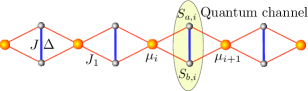
Figure 1: (Color online) Schematic representation of Ising-$XXZ$ diamond chain. The blue line represents the bipartite quantum coupling which serves as a quantum channel. The red line corresponds to Ising spin couplings.

We consider as a quantum channel the Ising-$XXZ$ model with nodal Ising spins and anisotropic Heisenberg spins on a diamond-like chain in the presence of an external magnetic field, schematically illustrated in Fig. 1. Thus, the corresponding Hamiltonian operator can be expressed as follow

$$\mathcal{H}= \sum_{i=1}^{N}[J\left(\boldsymbol{S}_{a,i},\boldsymbol{S}_{b,i}\right)_{\Delta}+J_{1}\left(S_{a,i}^{z}+S_{b,i}^{z}\right)\left(\mu_{i}+\mu_{i+1}\right)+$$

$$-h\left(S_{a,i}^{z}+S_{b,i}^{z}\right)-\frac{h}{2}\left(\mu_{i}+\mu_{i+1}\right)],$$ (1)

where $\left(\boldsymbol{S}_{a,i},\boldsymbol{S}_{b,i}\right)_{\Delta}=S_{a,i}^{x}S_{b,i}^{x}+S_{a,i}^{y}S_{b,i}^{y}+\Delta S_{a,i}^{z}S_{b,i}^{z}$ corresponds to the interstitial anisotropic Heisenberg spins coupling $J$ and $\Delta$, whereas the nodal-interstitial spins $\mu_{i}$ are representing the Ising-type exchanges $J_{1}$. The system is under longitudinal external magnetic field $h$ acting on Heisenberg spins and Ising spins.

The quantum Heisenberg spin coupling can be expressed using matrix notation in the standard basis $\{|\uparrow\uparrow\rangle,|\uparrow\downarrow\rangle,|\downarrow\uparrow\rangle,|\downarrow\downarrow\rangle\}$, where $|\uparrow\rangle$ and $|\downarrow\rangle$ denote the spin-up and spin-down states, respectively. Thus, we have

$$\left(\boldsymbol{S}_{a,i},\boldsymbol{S}_{b,i}\right)_{\Delta}=\left[\begin{array}[]{cccc}\frac{\Delta}{4}&0&0&0\\ 0&-\frac{\Delta}{4}&\frac{1}{2}&0\\ 0&\frac{1}{2}&-\frac{\Delta}{4}&0\\ 0&0&0&\frac{\Delta}{4}\end{array}\right],$$ (2)

and

$$S_{a,i}^{z}+S_{b,i}^{z}=\left[\begin{array}[]{cccc}1&0&0&0\\ 0&0&0&0\\ 0&0&0&0\\ 0&0&0&-1\end{array}\right].$$ (3)

Thus, we obtain the following eigenvalues after the diagonalization of Heisenberg spins dimer (sites $a$ and $b$), and assuming fixed values for $\mu_{i}$ and $\mu_{i+1}$, we have

$$\mathcal{E}_{1}(\mu_{i},\mu_{i+1})= \frac{J\Delta}{4}+\left(J_{1}-\frac{h}{2}\right)\left(\mu_{i}+\mu_{i+1}\right)-h,$$

$$\mathcal{E}_{2}(\mu_{i},\mu_{i+1})= \frac{J}{2}-\frac{J\Delta}{4}-\frac{h}{2}\left(\mu_{i}+\mu_{i+1}\right),$$

$$\mathcal{E}_{3}(\mu_{i},\mu_{i+1})= -\frac{J}{2}-\frac{J\Delta}{4}-\frac{h}{2}\left(\mu_{i}+\mu_{i+1}\right),$$

$$\mathcal{E}_{4}(\mu_{i},\mu_{i+1})= \frac{J\Delta}{4}-\left(J_{1}+\frac{h}{2}\right)\left(\mu_{i}+\mu_{i+1}\right)+h.$$ (4)

Where their corresponding eigenstates are obtained using standard basis respectively by

$$|\varphi_{1}\rangle= |\uparrow\uparrow\rangle,$$ (5)

$$|\varphi_{2}\rangle= \frac{1}{\sqrt{2}}\left(|\uparrow\downarrow\rangle+|\downarrow\uparrow\rangle\right),$$ (6)

$$|\varphi_{3}\rangle= \frac{1}{\sqrt{2}}\left(|\uparrow\downarrow\rangle-|\downarrow\uparrow\rangle\right),$$ (7)

$$|\varphi_{4}\rangle= |\downarrow\downarrow\rangle.$$ (8)

II.1 Quantum channel density operator

The Ising-$XXZ$ diamond chain was recently studied mrojas , through a decoration transformation phys-A-09-1 ; strecka pla-1 and a transfer-matrix approach baxter-book-1 .

Guided by that solution, the local density operator for dimer operator (site $a$ and $b$) bonded by Ising particles $\mu$ and $\mu^{\prime}$, can be expressed by

$$\varrho(\mu,\mu^{\prime})=\sum_{i=1}^{4}\mathrm{e}^{-\beta\varepsilon_{i}(\mu,\mu^{\prime})}|\varphi_{i}\rangle\langle\varphi_{i}|.$$ (9)

Here, $\beta=1/(k_{B}T)$, $k_{B}$ is being the Boltzmann‘s, constant and $T$ being the absolute temperature.

Thus, the density operator in the natural basis can be expressed by

$$\varrho=\left[\begin{array}[]{cccc}\varrho_{1,1}&0&0&0\\ 0&\varrho_{2,2}&\varrho_{2,3}&0\\ 0&\varrho_{3,2}&\varrho_{3,3}&0\\ 0&0&0&\varrho_{4,4}\end{array}\right],$$ (10)

where the elements of the two qubits operator are

$$\varrho_{1,1}(\mu,\mu^{\prime})= \mathrm{e}^{-\beta\varepsilon_{1}(\mu,\mu^{\prime})},$$

$$\varrho_{2,2}(\mu,\mu^{\prime})= \frac{1}{2}\left(\mathrm{e}^{-\beta\varepsilon_{2}(\mu,\mu^{\prime})}+\mathrm{e}^{-\beta\varepsilon_{3}(\mu,\mu^{\prime})}\right),$$

$$\varrho_{2,3}(\mu,\mu^{\prime})= \frac{1}{2}\left(\mathrm{e}^{-\beta\varepsilon_{2}(\mu,\mu^{\prime})}-\mathrm{e}^{-\beta\varepsilon_{3}(\mu,\mu^{\prime})}\right),$$

$$\varrho_{4,4}(\mu,\mu^{\prime})= \mathrm{e}^{-\beta\varepsilon_{4}(\mu,\mu^{\prime})}.$$ (11)

II.2 Average density operator of Heisenberg spin dimer

Following the result obtained in reference mrojas , the average density operator of Heisenberg spin dimer, is given by

$$\rho_{ch}=\left[\begin{array}[]{cccc}\rho_{1,1}&0&0&0\\ 0&\rho_{2,2}&\rho_{2,3}&0\\ 0&\rho_{3,2}&\rho_{3,3}&0\\ 0&0&0&\rho_{4,4}\end{array}\right],$$ (12)

where elements of quantum channel density operator, in the thermodynamic limit, are expressed

$$\rho_{i,j}= \frac{1}{\Lambda_{+}}\left\{\tfrac{\varrho_{i,j}(\tfrac{1}{2},\tfrac{1}{2})+\varrho_{i,j}(-\tfrac{1}{2},-\tfrac{1}{2})}{2}+\tfrac{2\varrho_{i,j}(\tfrac{1}{2},-\tfrac{1}{2})w_{+-}}{\sqrt{\left(w_{++}-w_{--}\right)^{2}+4w_{+-}^{2}}}\right.$$

$$\left.+\tfrac{\left(\varrho_{i,j}(\tfrac{1}{2},\tfrac{1}{2})-\varrho_{i,j}(-\tfrac{1}{2},-\tfrac{1}{2})\right)\left(w_{++}-w_{--}\right)}{2\sqrt{\left(w_{++}-w_{--}\right)^{2}+4w_{+-}^{2}}}\right\}.$$ (13)

where the Boltzmann factor is given by

$$w(\mu,\mu^{\prime})=\mathrm{tr}_{ab}\left(\varrho(\mu,\mu^{\prime})\right)=\sum_{i=1}^{4}\mathrm{e}^{-\beta\varepsilon_{i}(\mu,\mu^{\prime})}.$$ (14)

Defining conveniently $w_{\pm\pm}\equiv w(\pm\frac{1}{2},\pm\frac{1}{2})$ and $w_{+-}\equiv w(\frac{1}{2},-\frac{1}{2})$. Whereas, $\Lambda_{+}$ is the largest eigenvalue

$$\Lambda_{+}=\tfrac{w_{++}+w_{--}+\sqrt{\left(w_{++}-w_{--}\right)^{2}+4w_{+-}^{2}}}{2}.$$ (15)

The average density operator (12) of Heisenberg spin dimer, will be useful to study quantum teleportation through the Heisenberg dimers.

III Entangled state teleportation

In this section, we study the quantum teleportation using as quantum channel a couple of Heisenberg dimer in the Ising-Heisenberg diamond chain discussed above, considering the standard teleportation protocol Bennet . The couple of quantum channels are considered sufficiently far away from each other, thus we ignore any possible coupling between each diamond chains. The standard teleportation of two qubits through a mixed entangled state; can be viewed as a generalized depolarizing channel bowen ; horo . The input state $\rho_{in}=|\psi_{in}\rangle\langle\psi_{in}|$ depicted in figure 2 is destroyed and its output state $\rho_{out}$ appears on another side of the diamond chain after applying a local measurement in the form of linear operators.

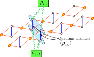
Figure 2: Schematic representation for teleportation of input state $\rho_{in}$, through a couple of independent Heisenberg dimers (blue lines) in an Ising-Heisenberg diamond chain, and the teleported output state is denoted by $\rho_{out}$.

Let us consider an initial state of two qubits in the natural basis of qubits $\{|0\rangle,|1\rangle\}$, note that this basis cannot be confused with Heisenberg dimer natural basis, defined previously. Thus, the initial unknown pure state is expressed by

$$\begin{array}[]{ccc}\mid\psi_{in}\rangle&=&\cos(\frac{\theta}{2})|10\rangle+{\rm e}^{i\phi}\sin(\frac{\theta}{2})|01\rangle,\end{array}$$ (16)

where $0\leqslant\theta\leqslant\pi$ and $0\leqslant\phi\leqslant 2\pi$. Here, $\theta$ describes an arbitrary state and $\phi$ is the corresponding phase of this state.

Surely, the initial state $\rho_{in}$ concurrence, can be obtained easily, which becomes

$$\mathcal{C}_{in}=2\left|e^{i\phi}\sin\left(\tfrac{\theta}{2}\right)\cos\left(\tfrac{\theta}{2}\right)\right|=|\sin\left(\theta\right)|.$$ (17)

To study the output state $\rho_{out}$, we need to use the well known Bell states given by

$$|\Phi^{\pm}\rangle= \tfrac{1}{\sqrt{2}}\left(|00\rangle\pm|11\rangle\right),$$ (18)

$$|\Psi^{\pm}\rangle= \tfrac{1}{\sqrt{2}}\left(|01\rangle\pm|10\rangle\right),$$ (19)

with these states, we can construct the projection operator for each Bell states: $E^{0}=|\Psi^{-}\rangle\langle\Psi^{-}|$, $E^{1}=|\Phi^{-}\rangle\langle\Phi^{-}|$, $E^{2}=|\Phi^{+}\rangle\langle\Phi^{+}|$ and $E^{3}=|\Psi^{+}\rangle\langle\Psi^{+}|$. Besides, the probability to find a Bell state is given by $p_{i}={\rm tr}\left[E^{i}\rho_{ch}\right]$. Obviously, we can verify that $\underset{i}{\sum}p_{i}=1$.

Therefore, it is possible to express the output state $|\rho_{out}\rangle$ using the density operator bowen defined by,

$$\rho_{out}=\underset{i,j=\{0,x,y,z\}}{\sum}p_{i}p_{j}(\sigma_{i}\otimes\sigma_{j})\rho_{in}(\sigma_{i}\otimes\sigma_{j}),$$ (20)

where $\sigma_{0}$ is the identity matrix and $\sigma_{\alpha}$ $(\alpha=x,y,z)$ are the three components of the Pauli matrices.

Now, let us express the elements of density operator $\rho_{out}$, which has the following structure

$$\rho_{out}=\left[\begin{array}[]{cccc}\alpha&0&0&0\\ 0&a&b&0\\ 0&b^{*}&d&0\\ 0&0&0&\alpha\end{array}\right].$$ (21)

Where the elements of average density operator can be expressed by,

$$\alpha=\> 2\rho_{2,2}\left(\rho_{1,1}+\rho_{4,4}\right),$$

$$a=\> \left(\rho_{1,1}+\rho_{4,4}\right)^{2}\cos^{2}\left(\tfrac{\theta}{2}\right)+4\rho_{2,2}^{2}\sin^{2}\left(\tfrac{\theta}{2}\right),$$

$$b=\> 2e^{i\phi}\rho_{2,3}^{2}\sin\theta,$$

$$d=\> 4\rho_{2,2}^{2}\cos^{2}\left(\tfrac{\theta}{2}\right)+\left(\rho_{1,1}+\rho_{4,4}\right)^{2}\sin^{2}\left(\tfrac{\theta}{2}\right).$$ (22)

To describe the thermal entanglement of the output state $\rho_{out}$, we use the concurrence defined by Wootters wootters ; hill , which is given by

$$\mathcal{C}_{out}=\mathrm{max}\{\sqrt{\lambda_{1}}-\sqrt{\lambda_{2}}-\sqrt{\lambda_{3}}-\sqrt{\lambda_{4}},0\},$$ (23)

assuming $\lambda_{i}$ are the eigenvalues in decreasing order of the matrix

$$R_{out}=\rho_{out}\left(\sigma^{y}\otimes\sigma^{y}\right)\rho_{out}^{*}\left(\sigma^{y}\otimes\sigma^{y}\right),$$ (24)

where $\rho_{out}^{*}$ denotes the complex conjugation of $\rho_{out}$.

It is easy to show, that the eigenvalues of Eq. (24), are given by

$$\lambda_{1(2)}= \left(\sqrt{ad}\pm\sqrt{bb^{*}}\right)^{2},\; \lambda_{3(4)}=\alpha^{2},$$ (25)

with

$$ad= \left(\tfrac{\left(\rho_{1,1}+\rho_{4,4}\right)^{2}}{2}+2\rho_{2,2}^{2}\right)^{2}-$$

$$\left(\tfrac{\left(\rho_{1,1}+\rho_{4,4}\right)^{2}}{2}-2\rho_{2,2}^{2}\right)^{2}\left(1-\mathcal{C}_{in}^{2}\right),$$ (26)

$$bb^{*}= 4\rho_{2,3}^{4}\mathcal{C}_{in}^{2}.$$ (27)

Using the result Eq. (25), the concurrence of the output state can be obtained from Eq. (23), which results in

$$\mathcal{C}_{out}=2\mathrm{max}\left\{2\rho_{2,3}^{2}\mathcal{C}_{in}-2\mid\rho_{2,2}\mid\mid\rho_{1,1}+\rho_{4,4}\mid,0\right\}.$$ (28)

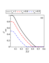
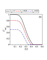
Figure 3: (Color online) Output concurrence $\mathcal{C}_{out}$ as a function of $T/J$ for $J_{1}/J=1$, $\Delta=1.5$ and different values of $\mathcal{C}_{in}$. In (a) we display $\mathcal{C}_{out}$ in the absence of the magnetic field and in (b) we display $\mathcal{C}_{out}$ for magnetic field $h/J=1$.

In what follows, study the effects of the output entanglement as a function of the concurrence and quantum channel condition (the Ising-Heisenberg parameters). In Fig. 3(a) is illustrated the output concurrence $\mathcal{C}_{out}$ as a function of the $T/J$ for different values of input concurrence $\mathcal{C}_{in}$, assuming null magnetic field. We observe the output concurrence decreases as soon as the temperature increases and for temperature higher than the threshold temperature, the output concurrence becomes null indicating there is no entanglement for temperature above than threshold temperature. In the low-temperature limit, we can also observe the output concurrence and input concurrence is closely related. Whereas, in Fig. 3(b) is illustrated for $h/J=1$, observing the output concurrence is enhanced in the low temperature region due to de presence of magnetic field. Although for higher temperature the entanglement is also destroyed.

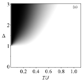
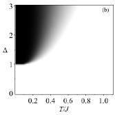
Figure 4: Density plot of output concurrence $\mathcal{C}_{out}$ as a function of $T/J$ and $\Delta$. In (a) we display $\mathcal{C}_{out}$ in the absence of the magnetic field. In (b) we display $\mathcal{C}_{out}$ for $h/J=1$, the black (white) region corresponds to $\mathcal{C}_{out}=1(0)$ and by gray regions we indicate a concurrence $0<\mathcal{C}_{out}<1$.

Now we can start our discussion regarding quantum teleportation of the entangled input state. From Eq. (28) we can analyze the behavior of teleported state $\rho_{out}$, for a range of parameters assuming the state $\rho_{in}$ is maximally entangled ($\theta=\pi/2$).

In Fig. 4, we illustrate the density plot of output concurrence $\mathcal{C}_{out}$ as a function of $T/J$ and $\Delta$ for a fixed value of $J_{1}/J$=1. The black region corresponds to the maximum entangled region ($\mathcal{C}_{out}=1$), whereas the white region corresponds to the unentangled region ($\mathcal{C}_{out}=0$). The gray region means the different degrees of entanglement ($0<\mathcal{C}_{out}<1$). In Fig. 4(a) it is shown that the model is maximally entangled only for $\Delta\geqslant 1$ in the absence of the magnetic field, while the concurrence $\mathcal{C}_{out}$ is always null for $\Delta<1$. The concurrence $\mathcal{C}_{out}$ becomes smaller when increasing the temperature and as expected the entanglement vanishes at high temperature. In Fig. 4(b), we display $\mathcal{C}_{out}$ for $h/J=1$, where the concurrence behaves similar to Fig. 4(a), also the concurrence is enhanced up to higher temperature.

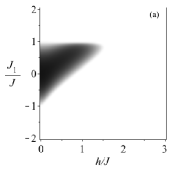
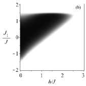
Figure 5: Density plot of output concurrence $\mathcal{C}_{out}$ as a function of $h/J$ and $J_{1}/J$ . In (a) we display of $\Delta=1$ and in (b) is for $\Delta=2$.

In Fig. 5 is shown another density plot of concurrence $\mathcal{C}_{out}$ as a function of magnetic field $h/J$ and $J_{1}/J$. To represent the concurrence, we use the same representation as in Fig. 4, assuming fixed value of $T/J=0.2$. In Fig. 5(a), we display $\mathcal{C}_{out}$ for $\Delta=1$, thus, we can illustrate that the concurrence is always less than $\mathcal{C}_{out}\lesssim 0.9$. The largest concurrence occurs for $|J_{1}/J|\lesssim 1$ and magnetic field $h/J\lesssim 1.5$. Whereas, in Fig. 5(b), we display $\mathcal{C}_{out}$ for $\Delta=2$, and we observe that, the output concurrence is enhanced by increasing the anisotropy $\Delta$. Therefore, the teleportation is more efficient in the environment with a high magnetic field and strong anisotropy parameter of Ising-Heisenberg chain (quantum channel condition).

IV Fidelity of entangled state teleportation

To describe the quality of the process of teleportation, it is quite relevant to study the fidelity between $\rho_{in}$ and $\rho_{out}$ to characterizes the success of teleported state. When the input state is a pure state, we can apply the concept of fidelity as a useful indicator of teleportation performance of a quantum channel. The fidelity of $\rho_{out}$ was defined Joz as

$$F = \langle\psi_{in}|\rho_{out}|\psi_{in}\rangle,$$ (29)

$$= \left\{{\rm tr}\left[\sqrt{\sqrt{\rho_{in}}\rho_{out}\sqrt{\rho_{in}}}\right]\right\}^{2}.$$

After a straightforward calculation, the fidelity becomes

$$F=\tfrac{\sin^{2}\theta}{2}\left[\left(\rho_{1,1}+\rho_{4,4}\right)^{2}+4\rho_{2,3}^{2}-4\rho_{2,2}^{2}\right]+4\rho_{2,2}^{2}.$$ (30)

When the input state is a pure state, the efficiency of quantum communication is characterized by the average fidelity Joz . The average fidelity $F_{A}$ of teleportation can be formulated as

$$F_{A}=\frac{1}{4\pi}\intop_{0}^{2\pi}d\phi\intop_{0}^{\pi}F\sin\theta d\theta.$$ (31)

After integrating the average fidelity $F_{A}$ we obtain

$$F_{A}=\frac{1}{3}\left[\left(\rho_{1,1}+\rho_{4,4}\right)^{2}+4\rho_{2,3}^{2}-4\rho_{2,2}^{2}\right]+4\rho_{2,2}^{2}.$$ (32)

To transmit a quantum state $|\psi_{in}\rangle$ better than any classical communication protocol, $F_{A}$ must be greater than $\frac{2}{3}$ which is the best fidelity in the classical world Joz .

To describe the behavior of the average fidelity in the standard teleportation protocol, some plots are given below.

In Fig. 6 we depict the average fidelity as a function of $\Delta$ and $T/J$ for a fixed value of $J_{1}/J=1$. The black region correspond to the maximum average fidelity $\left(F_{A}=1\right)$, while the white region corresponds to $F_{A}=0$. The yellow curve surrounding the dark region ($F_{A}>2/3$) means the region in which the quantum teleportation will become successful, whereas the outside means the quantum teleportation fails and becoming classical communication region. From Fig. 6(a), we can see that when $\Delta\geqslant 1$ the average fidelity is maximum in the absence of magnetic field, while for $\Delta<1$ the average fidelity is always less than or equal to $2/3$. In Fig. 6(b), we display $F_{A}$ for $h/J=1$, where the average fidelity behaves similar to Fig. 6(a). However, the Fig. 6(b) clearly shows that, when $\Delta\thickapprox 1$ and at temperatures less than $T/J\approx 0.1$, the average fidelity is maximum.

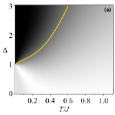
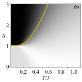
Figure 6: Density plot average of fidelity $F_{A}$ as a function of $T/J$ versus $\Delta$ for $J_{1}/J=1.0$. In (a) we display $F_{A}$ for a $h/J=0$ and in (b) we display $F_{A}$ for $h/J=1$. For both figures, the yellow curve is the contour for $F_{A}=2/3$.

In Fig. 7, we show the properties of the average fidelity $F_{A}$ versus parameter $J_{1}/J$ and magnetic field $h/J$. From the Fig. 7(a), we note that the average fidelity becomes $F_{A}>\frac{2}{3}$ for $|\frac{J_{1}}{J}|\lesssim 0.84$ and magnetic field $h/J\lesssim 1.33$. In Fig. 7 (b), it is shown that the model is acceptable for teleportation when $|\frac{J_{1}}{J}|\lesssim 1.33$ and $\frac{h}{J}\lesssim 2.35$. Similar to the previous case, the surrounding yellow curve is the boundary between quantum teleportation would be successful or not.

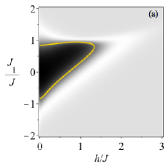
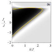
Figure 7: Density plot of average fidelity $F_{A}$ as a function of $h/J$ versus $J_{1}/J$ for $T/J=0.2$. (a) $\Delta=1$. (b) $\Delta=2$. For both figures, the yellow curve is the contour for $F_{A}=2/3$.

On the other hand, in Fig. 8 is shown the average fidelity $F_{A}$ as a function of the temperature $T/J$ for different values of $h/J$ and $\Delta$, assuming fixed values $J_{1}/J=1$. In the figures the horizontal dashed lines at $F_{A}=2/3$ denote the limit of quantum fidelities. The Fig. 8(a) shows clearly that, the magnetic field can enhance the average fidelity in interval $0\leqslant h/J<2.5$. Furthermore, the plot also shows that when increasing the magnetic field $h/J\geqslant 2.5$, the teleportation will not succeed since $F_{A}\leqslant 2/3$. This occurs because the systems is in the interphase between the entangled state and the unentangled state at zero temperature (see Ref. mrojas ). Whereas, in Fig. 8(b), we can notice that the average fidelity gradually decreases below $2/3$, when increases $\Delta$ up to $\Delta=1$. For $\Delta=1.1$, the average fidelity leads to a fixed value $1$, in the low temperature region, when temperature increases, the value of $F_{A}$ quickly decays below $2/3$. With the increase of the anisotropy parameter to $\Delta=3$, the average fidelity $F_{A}$ enhances and then decreases monotonically as soon as the $T/J$ increase. Thus, we conclude the quantum teleportation protocol will succeed for large $\Delta$ and for a given magnetic field.

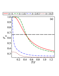
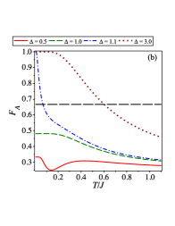
Figure 8: (Color online) Average fidelity $F_{A}$ is plotted as a function of the temperature $T/J$ for $J_{1}/J=1$. (a) For $\Delta=2$. (b) For $h/J=0$. Horizontal dashed line indicates the 2/3 constant line.

Furthermore, to illustrate the effect of the magnetic field $h/J$ on the average fidelity, we plot $F_{A}$ as a function of $h/J$ at different temperature $T/J$. In Fig. 9(a), we can observe that for $\Delta=1.1$, the average fidelity is constant and equal to $F_{A}=1$, for temperature close to zero $T/J=0.01$, and then drops suddenly to $F_{A}\approx 0.25$ at a critical value $h/J=2.06$. For $h/J>2.06$, the average fidelity gains an asymptotic revitalization up to $F_{A}\rightarrow 1/3$, after reaching to its minimum value. For temperature $T/J\gtrsim 0.1$ the average fidelity is less than $2/3$ in $h/J=0$. When the magnetic field is introduced, the average fidelity attain the maximum and then, the average fidelity $F_{A}$ decreases leading to $F_{A}\approx 0.25$. However, there is a revival of average fidelity reaching value $F_{A}\rightarrow 1/3$.

On the other hand, we can observe clearly that when $T/J\geq 0.3$, the average fidelity is always smaller than $2/3$. In Fig. 9(b), we plot the average fidelity as a function of the magnetic field, for $\Delta=2$. One can find when $T/J$ is equal to $0.5$, it is no longer possible to observe the quantum communication in absence of magnetic field $h/J=0$. Here, the average fidelity also presents the same interesting feature, the curves almost vanishes and recovery the average fidelity for a particular value of the magnetic field $h$. After achieving the minimum value, the average fidelity increases monotonically when increasing the magnetic field up to $F_{A}\rightarrow 1/3$.

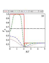
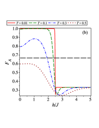
Figure 9: (Color online) Average fidelity $F_{A}$ is plotted as a function of the magnetic field $h/J$ for different values of temperature and $J_{1}/J=1$. (a) For $\Delta=1.1$. (b) For $\Delta=2$. Horizontal dashed line indicates the 2/3 constant line.

Finally, to observe the effects of output concurrences and average fidelity of quantum teleportation. We plot the quantum channel concurrence $\text{$\mathcal{C}$}_{ch}$ (yellow curves), output concurrence $\mathcal{C}_{out}$ (red curves) and average fidelity $F_{A}$ (black curves) as a function of temperature $T/J$ for different values of the $h/J$ and $\Delta$. In Fig. 10(a) are displayed $\text{$\mathcal{C}$}_{ch}$, $\text{$\mathcal{C}$}_{out}$ and $F_{A}$ versus $T/J$. For null magnetic field $h/J=0$ and fixed $\Delta=1.1$ (solid lines), the quantum channel concurrence and output concurrence disappears in the threshold temperature $T_{th}/J\approx 0.74$ and $T_{th}/J\approx 0.3$ respectively. While the average fidelity is successful up to temperature $T/J\approx 0.1$, and $F_{A}$ gradually decreases when increases $T/J$ until reaching $F_{A}\approx 0.25$. For $\Delta=2$ (dashed line), the quantum channel concurrence $\text{$\mathcal{C}$}_{ch}$ vanishes for $T_{th}/J\gtrapprox 1.07$. The threshold temperature for output concurrence $\text{$\mathcal{C}$}_{out}$ occurs at $T_{th}/J\gtrapprox 0.58$. It is also observed that the quantum communication is enhanced with the increase of $\Delta$ ($F_{A}>\frac{2}{3}$, represented as dash-doted line). On the other hand, for higher temperature, $F_{A}$ decays monotonically and it approaches to $0.25$. In Fig. 10(b) for a fixed value of $h/J=2$, we display $\text{$\mathcal{C}$}_{ch}$, $\text{$\mathcal{C}$}_{out}$ and $F_{A}$ as functions of $T/J$ and fixed $\Delta=1.1$ (solid lines). One can notice that, the quantum channel concurrence and output concurrence disappears in the threshold temperature $T_{th}/J\approx 0.84$ and $T_{th}/J\approx 0.043$ respectively. While $F_{A}$ decreases monotonically until $F_{A}\approx 0.25$ as soon as the temperature increases. On the other hand, for $\Delta=2$ (dashed lines) the threshold temperature for $\text{$\mathcal{C}$}_{ch}$ is $T_{th}/J=1.12$ and for $\text{$\mathcal{C}$}_{out}$ becomes $T_{th}/J=0.37$. However the average fidelity leads asymptotically to $F_{A}\approx 0.25$.

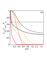
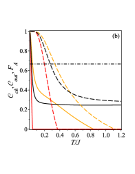
Figure 10: (Color online) Comparison of quantum channel concurrence (yellow), output concurrence (red) and average fidelity (black) versus $T/J$ for $J_{1}/J=1$, $\Delta=1.1$ (solid line) and $\Delta=2$ (dashed line). (a) For $h/J=0$. (b) For $h/J=2$. Horizontal dashed line indicates the 2/3 constant line.

V Conclusions

In this article, we have studied the quantum teleportation of two qubits. The quantum teleportation performing through a quantum channel composed by a couple of Heisenberg dimers in an Ising-$XXZ$ diamond chain structure. When the input state is a pure state, we can apply the concept of fidelity as a useful quantity to study the of teleportation performance by a quantum channel horo . Assuming the teleported qubits in an arbitrary state, we have obtained analytical results for the quantum channel concurrence, output concurrence, and the average fidelity. We discussed in detail the effects of coupling parameters of the Ising-Heisenberg diamond chain (quantum channel), as a function of magnetic field and temperature dependence for the output concurrence, quantum channel concurrence, and average fidelity. Displaying the results as a function of the anisotropy coupling $\Delta$ and external magnetic field $h$. Therefore, we observe the magnetic field $h$ and the anisotropy parameter $\Delta$ influence strongly in the output concurrence and average fidelity. Thus, when the magnetic field increased, the output concurrence is stimulated favoring the teleportation success for a larger region. However, for a sufficiently strong magnetic field, the output concurrence gradually decreases, and the entangled state teleportation will not succeed anymore. In figures 6 and 7 have illustrated this effect, the darkest region contoured by a solid line shows the region in which the quantum teleportation could well succeed, whereas for the outside of this curves means the quantum teleportation would fail.

On the other hand, we observe the quantum teleportation increases when increases of anisotropy parameter $\Delta$, then we conclude the parameter $\Delta$ is the more efficient control parameter of quantum communications illustrated in figures 9 and 10.

References

• (1) L. Amico, R. Fazio, A. Osterloh and V. Vedral, Rev. Mod. Phys. 80, 517 (2008); R. Horodecki et al., Rev. Mod. Phys. 81, 865 (2009); O. GΓΌhne and G. TΓ³th, Phys. Rep. 474, 1 (2009).
• (2) K. M. O’Connor and W. K. Wootters, Phys. Rev. A 63, 052302 (2001); Y. Sun, Y. Chen and H. Chen, Phys. Rev. A 68, 044301 (2003); G. L. Kamta and A. F. Starace, Phys. Rev. Lett. 88, 107901 (2002).
• (3) C. H. Bennett, G. Brassard, S. CrΓ©peau, R. Jozsa, A. Peres and W. K. Wootters, Phys. Rev. Lett. 70, 1895 (1993).
• (4) S. Popescu, Phys. Rev. Lett. 72, 797 (1994); M. Horodecki, P. Horodecki and R. Horodecki, Phys. Rev. A 60, 1888 (1999).
• (5) D. Bouwmeester, J. W. Pan, K. Mattle, M. Eibl, H. Weinfurter and A. Zeilinger, Nature (London) 390, 575 (1997); D. Boschi, S. Branca, F. de Martini, L. Hardy and S. Popescu, Phys. Rev. Lett. 80, 1121 (1998).
• (6) Y. Yeo, Phys. Rev. A 66, 062312 (2002); G. F. Zhang, Phys. Rev. A 75, 034304 (2007); F. Kheirandish, S. J. Akhtarshenas and H. Mohammadi, Phys. Rev. A 77, 042309 (2008); Y. Zhou, G. F. Zhang, Euro. Phys. J. D 47, 227 (2008).
• (7) Wan Qin and Jin-Liang Guo, Int. J. Theor. Phys. 54, 2386 (2015).
• (8) H. Kikuchi, Y. Fujii, M. Chiba, S. Mitsudo, T. Idehara, T. Tonegawa, K. Okamoto, T. Sakai, T. Kuwai, and H. Ohta, Phys. Rev. Lett. 94, 227201 (2005).
• (9) A. Honecker and A. Lauchli. Phys. Rev. B 63, 174407 (2001); H. Jeschke et al., Phys. Rev. Lett. 106, 217201 (2011); N. Ananikian, H. Lazaryan, and M. Nalbandyan, Eur. Phys. J. B 85, 223 (2012).
• (10) A. Honecker, S. Hu, R. Peters J. Ritcher, J. Phys.: Condens. Matter 23, 164211 (2011).
• (11) L. Canova, J. Strecka, and M. Jascur, J. Phys: Condens. Matter 18, 4967 (2006).
• (12) O. Rojas, S. M. de Souza, V. Ohanyan, M. Khurshudyan, Phys. Rev. B 83 , 094430 (2011).
• (13) J. S. Valverde, O. Rojas, S. M. de Souza, J. Phys. Condens. Matter 20, 345208 (2008); O. Rojas, S. M. de Souza, Phys. Lett. A 375, 1295 (2011).
• (14) B. M. Lisnii, Ukrainian Journal of Physics 56, 1237 (2011).
• (15) O. Rojas, M. Rojas, N. S. Ananikian and S. M. de Souza, Phys. Rev. A 86, 042330 (2012).
• (16) J. Torrico, M. Rojas, S. M. de Souza, Onofre Rojas and N. S. Ananikian, Europhysics Letters 108, 50007 (2014).
• (17) J. Torrico, M. Rojas, M. S. S. Pereira, J. Strecka and M. L. Lyra, Phys. Rev. B 93, 014428 (2016).
• (18) O. Rojas, J. S. Valverde, S. M. de Souza, Physica A 388, 1419 (2009); O. Rojas, S. M. de Souza, J. Phys. A: Math. Theor. 44, 245001 (2011).
• (19) J. Strečka, Phys. Lett. A 374, 3718 (2010).
• (20) R. J. Baxter, Exactly Solved Models in Statistical Mechanics, (Academic Press, New York, 1982).
• (21) W. K. Wootters, Phys. Rev. Lett. 80, 2245 (1998).
• (22) S. Hill and W. K. Wootters, Phys. Rev. Lett. 78, 5022 (1997).
• (23) G. Bowen and S. Bose, Phys. Rev. Lett. 87, 267901 (2001).
• (24) M. Horodecki, P. Horodecki and R. Horodecki, Phys. Rev. A 60, 1888 (1999).
• (25) R. Jozsa, J. Mod. Opt. 41, 2315 (1994); M. Bowdrey, A. Short, K. Banaszek and J. A. Jones, Phys. Lett. A 294, 258 (2002).