trlib: A vector-free implementation of the GLTR method for iterative solution of the trust region problem

Abstract

We describe trlib, a library that implements a variant of Gould’s Generalized Lanczos method (Gould et al. in SIAM J. Opt. 9(2), 504–525, 1999) for solving the trust region problem.

Our implementation has several distinct features that set it apart from preexisting ones. We implement both conjugate gradient (CG) and Lanczos iterations for assembly of Krylov subspaces. A vector- and matrix-free reverse communication interface allows the use of most general data structures, such as those arising after discretization of function space problems. The hard case of the trust region problem frequently arises in sequential methods for nonlinear optimization. In this implementation, we made an effort to fully address the hard case in an exact way by considering all invariant Krylov subspaces.

We investigate the numerical performance of trlib on the full subset of unconstrained problems of the CUTEst benchmark set. In addition to this, interfacing the PDE discretization toolkit FEniCS with trlib using the vector-free reverse communication interface is demonstrated for a family of PDE-constrained control trust region problems adapted from the OPTPDE collection.

Keywords: trust-region subproblem, iterative method, Krylov subspace method, PDE constrained optimization

AMS subject classification. 35Q90, 65K05, 90C20, 90C30, 97N90

1 Introduction

In this article, we are concerned with solving the trust region problem, as it frequently arises as a subproblem in sequential algorithms for nonlinear optimization.

For this, let $\mathcal{H}$ denote a Hilbert space with inner product $\langle\cdot,\cdot\rangle$ and norm $\|\cdot\|$. Then, $H:\mathcal{H}\to\mathcal{H}$ denotes a self-adjoint, bounded operator on $\mathcal{H}$. We assume that $H$ has compact negative part, which implies sequential weak lower semicontinuity of the mapping $x\mapsto\langle x,Hx\rangle$, cf. [25] for details and a motivation. In particular, we assume that self-adjoint, bounded operators $P$ and $K$ exist on $\mathcal{H}$, such that $H=P-K$, that $K$ is compact, and that $\langle x,Px\rangle\geq 0$ for all $x\in\mathcal{H}$. The operator $M:\mathcal{H}\to\mathcal{H}$ is self-adjoint, bounded and coercive such that it induces an inner product $\langle\cdot,\cdot\rangle_{M}$ with corresponding norm $\|\cdot\|_{M}$ via $\langle x,y\rangle_{M}:=\langle x,My\rangle$ and $\|x\|_{M}:=\sqrt{\langle x,x\rangle_{M}}$. Furthermore, let $\mathcal{X}\subseteq\mathcal{H}$ be a closed subspace.

The trust region subproblem we are interested in reads

$$\left\{\quad\begin{array}[]{cl}\displaystyle\min_{x\in\mathcal{H}}&\tfrac{1}{2}\langle x,Hx\rangle+\langle x,g\rangle\\ \textup{s.t.}&\|x\|_{M}\leq\Delta,\\ &x\in\mathcal{X},\end{array}\right.$$ (4)

with $g\in\mathcal{H}$, objective function $q(x):=\tfrac{1}{2}\langle x,Hx\rangle+\langle x,g\rangle$, and trust region radius $\Delta>0$. Usually we take $\mathcal{X}=\mathcal{H}$ but will also consider truncated versions where $\mathcal{X}$ is a finite dimensional subspace of $\mathcal{H}$.

Readers who are less comfortable with the function space setting may think of $H$ as a symmetric positive definite matrix, of $\mathcal{H}$ as $\mathbb{R}^{n}$, and of $M$ as the identity on $\mathbb{R}^{n}$ inducing the standard scalar product and the euclidean norm $\|\cdot\|_{2}$. We follow the convention to indicate coordinate vectors $\bm{x}\in\mathbb{R}^{n}$ with boldface letters.

Related Work

Trust Region Subproblems are an important ingredient in modern optimization algorithms as globalization mechanism. The monography [9] provides an exhaustive overview on Trust Region Methods for nonlinear programming, mainly for problems formulated in finite-dimensional spaces. For trust region algorithms in Hilbert spaces, we refer to [26, 51, 23, 52] and for Krylov subspace methods in Hilbert space [24]. In [1] applications of trust region subproblems formulated on Riemannian manifolds are considered. Recently, trust region-like algorithms with guaranteed complexity estimates in relation to the KKT tolerance have been proposed [5, 6, 10]. The necessary ingredients in the subproblem solver for the algorithm investiged by Curtis and Samadi [10] have been implemented in trlib as well.

Solution algorithms for trust region problems can be classified into direct algorithms that make use of matrix factorizations and iterative methods that access the operators $H$ and $M$ only via evaluations $x\mapsto Hx$ and $x\mapsto Mx$ or $x\mapsto M^{-1}x$. For the Hilbert space context, we are interested in the latter class of algorithms. We refer to [9] and the references therein for a survey of direct algorithms, but point out the algorithm of Moré and Sorensen [36] that will be used on a specific tridiagonal subproblem, as well as the work of Gould et al. [21], who use higher order Taylor models to obtain high order convergence results. The first iterative method was based on the conjugate gradient process, and was proposed independently by Toint [50] and Steihaug [49]. Gould et al. [19] proposed an extension of the Steihaug-Toint algorithm. There, the Lanczos algorithm is used to build up a nested sequence of Krylov spaces, and tri-diagonal trust region subproblems are solved with a direct method. This idea also forms the basis for our implementation. Hager [22] considers an approach that builds on solving the problem restricted to a sequence of subspaces that use SQP iterates to accelerate and ensure quadratic convergence. Erway et al. [13, 14] investigate a method that also builds on a sequence of subspaces built from accelerator directions satisfying optimality conditions of a primal-dual interior point method. In the methods of Steihaug-Toint and Gould, the operator $M$ is used to define the trust region norm and acts as preconditioner in the Krylov subspace algorithm. The method of Erway et al. allows to use a preconditioner that is independent of the operator used for defining the trust region norm. The trust region problem can equivalently be stated as generalized eigenvalue problem. Approaches based on this characterization are studied by Sorensen [48], Rendl and Wolkowicz [44], and Rojas et al. [46, 47].

Contributions

We introduce trlib which is a new vector-free implementation of the GLTR (Generalized Lanczos Trust Region) method for solving the trust region subproblem. We assess the performance of this implementation on trust region problems obtained from the set of unconstrained nonlinear minimization problems of the CUTEst benchmark library, as well as on a number of examples formulated in Hilbert space that arise from PDE-constrained optimal control.

Structure of the Article

The remainder of this article is structured as follows. In §2, we briefly review conditions for existence and uniqueness of minimizers. The GLTR methods for iteratively solving the trust region problem is presented in §3 in detail. Our implementation, trlib is introduced in §4. Numerical results for trust-region problems arising in nonlinear programming and in PDE-constrained control are presented in §5. Finally, we offer a summary and conclusions in §6.

2 Existence and Uniqueness of Minimizers

In this section, we briefly summarize the main results about existence and uniqueness of solutions of the trust region subproblem. We first note that our introductory setting implies the following fundamental properties:

Lemma 1 (Properties of (4)).

1. The mapping $x\mapsto\langle x,Hx\rangle$ is sequentially weakly lower semicontinuous, and Fréchet differentiable for every $x\in\mathcal{H}$.

2. The feasible set $\mathcal{F}:=\{x\in\mathcal{H}\,|\,\|x\|_{M}\leq\Delta\}$ is bounded and weakly closed.

3. The operator $M$ is surjective.

Proof.

$H{{}=P-K}$ with compact $K$, so (1) follows from [25, Thm 8.2]. Fréchet differentiability follows from boundedness of $H$. Boundedness of $\mathcal{F}$ follows from coercivity of $M$. Furthermore, $\mathcal{F}$ is obviously convex and strongly closed, hence weakly closed. Finally, (3) follows by the Lax-Milgram theorem [8, ex. 7.19]: By boundedness of $M$, there is $C>0$ with $|\langle x,My\rangle|\leq C\|x\|\,\|y\|$. The coercitivity assumption implies existence of $c>0$ such that $\langle x,Mx\rangle\geq c\|x\|^{2}$ for $x,y\in\mathcal{H}$. Then, $M$ satisfies the assumptions of the Lax-Milgram theorem. Given $z\in\mathcal{H}$, application of this theorem yields $\xi\in\mathcal{H}$ with $\langle x,M\xi\rangle=\langle x,z\rangle$ for all $x\in\mathcal{H}$. Thus $M\xi=z$. ∎

Lemma 2 (Existence of a solution).

Problem (4) has a solution.

Proof.

By Lemma 1, the objecive functional $q$ is sequentially weakly lower semicontinuous and the feasible set $\mathcal{F}$ is weakly closed and bounded, the claim follows then from a generalized Weierstrass Theorem [27, Ch. 7]. ∎

To present optimality conditions for the trust region subproblem, we first present a helpful lemma on the change of the objective function between two points on the trust region boundary.

Lemma 3 (Objective Change on Trust Region Boundary).

Let $x^{0},x^{1}\in\mathcal{H}$ with $\|x^{i}\|_{M}=\Delta$ for $i=0,1$ be boundary points of (4), and let $\lambda\geq 0$ satisfy $(H+\lambda M)x^{0}+g=0$. Then $d=x^{1}-x^{0}$ satisfies $q(x^{1})-q(x^{0})=\tfrac{1}{2}\langle d,(H+\lambda M)d\rangle$.

Proof.

Using $0=\|x^{1}\|^{2}_{M}-\|x^{0}\|^{2}_{M}=\langle x^{0}+d,M(x^{0}+d)\rangle-\langle x^{0},Mx^{0}\rangle=\langle d,Md\rangle+2\langle x^{0},Md\rangle$ and $g=-(H+\lambda M)x^{0}$ we find

$$q(x^{1})-q(x^{0}) =\tfrac{1}{2}\langle d,Hd\rangle+\langle d,Hx^{0}\rangle+\langle g,d\rangle=\tfrac{1}{2}\langle d,Hd\rangle-\overbrace{\lambda\langle x^{0},Md\rangle}^{-\tfrac{1}{2}\lambda\langle d,Md\rangle}$$

$$=\tfrac{1}{2}\langle d,(H+\lambda M)d\rangle.\qed$$

Necessary optimality conditions for the finite dimensional problem, see e.g. [9], generalize in a natural way to the Hilbert space context.

Theorem 4 (Necessary Optimality Conditions).

Let $x^{*}\in\mathcal{H}$ be a global solution of $(\textup{TR}(H,g,M,\Delta,\mathcal{H}))$. Then there is $\lambda^{*}\geq 0$ such that

1. $(H+\lambda^{*}M)x^{*}+g=0$,

2. $\|x^{*}\|_{M}-\Delta\leq 0$,

3. $\lambda^{*}(\|x^{*}\|_{M}-\Delta)=0$,

4. $\langle d,(H+\lambda^{*}M)d\rangle\geq 0$ for all $d\in\mathcal{H}$.

Proof.

Let $\sigma:\mathcal{H}\to\mathbb{R},\sigma(x):=\langle x,Mx\rangle-\Delta^{2}$, so that the trust region constraint becomes $\sigma(x)\leq 0$. The function $\sigma$ is Fréchet-differentiable for all $x\in\mathcal{H}$ with surjective differential provided $x\neq 0$ and satisfies constraint qualifications in that case. We may assume $x^{*}\neq 0$ as the theorem holds for $x^{*}=0$ (then $g=0$) for elementary reasons.

Now if $x^{*}$ is a global solution of $(\textup{TR}(H,g,M,\Delta,\mathcal{H}))$, conditions (a)–(c) are necessary optimality conditions, cf. [8, Thm 9.1].

To prove (d), we distinguish three cases:

• $\|x\|_{M}=\Delta$ and $d\in\mathcal{H}$ with $\langle d,Mx^{*}\rangle\neq 0$: Given such $d$, there is $\alpha\in\mathbb{R}\setminus\{0\}$ with $\|x^{*}+\alpha d\|_{M}=\Delta$. Using Lemma 3 yields $\langle d,(H+\lambda^{*}M)d\rangle=\tfrac{2}{\alpha^{2}}(q(x^{*}+\alpha d)-q(x^{*}))\geq 0$ since $x^{*}$ is a global solution.

• $\|x\|_{M}=\Delta$ and $d\in\mathcal{H}$ with $\langle d,Mx^{*}\rangle=0$: Since $x^{*}\neq 0$ and $M$ is surjective, there is $p\in H$ with $\langle p,Mx^{*}\rangle\neq 0$, let $d(\tau):=d+\tau p$ for $\tau\in\mathbb{R}$. Then $\langle d(\tau),Mx^{*}\rangle\neq 0$ for $\tau\neq 0$, by the previous case

  $$0 \leq\langle d(\tau),(H+\lambda^{*}M)d(\tau)\rangle$$

  $$=\langle d,(H+\lambda^{*}M)d\rangle+\tau\langle p,(H+\lambda^{*}M)d\rangle+\tau^{2}\langle p,(H+\lambda^{*}M)p\rangle.$$

  Passing to the limit $\tau\to 0$ shows $\langle d,(H+\lambda^{*}M)d\rangle\geq 0$.

• $\|x\|_{M}<\Delta$: Then $\lambda^{*}=0$ by (c). Let $d\in\mathcal{H}$ and consider $x(\tau)=x^{*}+\tau d$, which is feasible for sufficiently small $\tau$. By optimality and stationarity (a):

  $$0\leq q(x(\tau))-q(x^{*})=\tau\langle x^{*},Hd\rangle+\tfrac{\tau^{2}}{2}\langle d,Hd\rangle+\tau\langle g,d\rangle=\tfrac{\tau^{2}}{2}\langle d,Hd\rangle,$$

  thus $\langle d,Hd\rangle\geq 0$. ∎

Corollary 5 (Sufficient Optimality Condition).

Let $x^{*}\in\mathcal{H}$ and $\lambda^{*}\geq 0$ such that (a)–(c) of Thm. 4 hold and $\langle d,(H+\lambda^{*}M)d\rangle>0$ holds for all $d\in\mathcal{H}$. Then $x^{*}$ is the unique global solution of $(\textup{TR}(H,g,M,\Delta,\mathcal{H}))$.

Proof.

This is an immediate consequence of Lemma 3. ∎

3 The GLTR Method

The GLTR (Generalized Lanczos Trust Region) method is an iterative method to approximatively solve $(\textup{TR}(H,g,M,\Delta,\mathcal{H}))$ and has first been described in Gould et al. [19]. Our presentation follows the presentation there and only deviates in minor details.

In every iteration of the GLTR process, problem $(\textup{TR}(H,g,M,\Delta,\mathcal{H}))$ is restricted to the Krylov subspace $\mathcal{K}_{i}:=\text{span}\{(M^{-1}H)^{j}M^{-1}g\,|\,0\leq j\leq i\}$,

$$\left\{\quad\begin{array}[]{cl}\displaystyle\min_{x\in\mathcal{H}}&\tfrac{1}{2}\langle x,Hx\rangle+\langle x,g\rangle\\ \textup{s.t.}&\|x\|_{M}\leq\Delta,\\ &x\in\mathcal{K}_{i}.\end{array}\right.$$ (8)

The following Lemma relates solutions of (8) to those of $(\textup{TR}(H,g,M,\Delta,\mathcal{H}))$.

Lemma 6 (Solution of the Krylov subspace trust region problem).

Let $x^{i}$ be a global minimizer of (8) and $\lambda^{i}$ the corresponding Lagrange multiplier. Then $(x^{i},\lambda^{i})$ satisfies the global optimality conditions of $(\textup{TR}(H,g,M,\Delta,\mathcal{H}))$ (Thm. 4) in the following sense:

1. $(H+\lambda^{i}M)x^{i}+g\,\perp_{M}\,\mathcal{K}_{i}$,

2. $\|x^{i}\|_{M}-\Delta\leq 0$,

3. $\lambda^{i}(\|x^{i}\|_{M}-\Delta)=0$,

4. $\langle d,(H+\lambda^{i}M)d\rangle\geq 0$ for all $d\in\mathcal{K}_{i}$.

Proof.

(b)–(d) are immediately obtained from Thm. 4 as $\mathcal{K}_{i}\subseteq\mathcal{H}$ is a Hilbert space. Assertion (a) follows from $x^{\ast}=x^{i}+x^{\perp}$ with $x^{i}\in\mathcal{K}_{i}$, $x^{\perp}\perp\mathcal{K}_{i}$ and Thm. 4 for $x^{i}$. ∎

Solving problem $(\textup{TR}(H,g,M,\Delta,\mathcal{H}))$ may thus be achieved by iterating the following Krylov subspace process. Each iteration requires the solution of an instance of the truncated trust region subproblem (8).

input : $H$, $M$, $g$, $\Delta$, tol

output : $i$, $x^{i}$, $\lambda^{i}$

for $i\geq 0$ do

       Construct a basis for the $i$-th Krylov subspace $\mathcal{K}_{i}$

       Compute a representation of $q(x)$ restricted to $\mathcal{K}_{i}$

       Solve the subproblem (8) to obtain $(x^{i},\lambda^{i})$

       if $\|(H+\lambda^{i}M)x^{i}+g\|_{M^{-1}}\leq\texttt{tol}$ then return

      

end for

Algorithm 1 Krylov subspace process for solving $(\textup{TR}(H,g,M,\Delta,\mathcal{H}))$.

Algorithm 1 stops the subspace iteration as soon as $\|(H+\lambda^{i}M)x^{i}+g\|_{M^{-1}}$ is small enough. The norm $\|\cdot\|_{M^{-1}}$ is used in the termination criterion since it is the norm belonging to the dual of $(\mathcal{H},\|\cdot\|_{M})$ and the Lagrange derivative representation $(H+\lambda^{i}M)x^{i}+g$ should be regarded as element of the dual.

3.1 Krylov Subspace Buildup

In this section, we present the preconditioned conjugate gradient (pCG) process and the preconditioned Lanczos process (pL) for construction of Krylov subspace bases. We discuss the transition from pCG to pL upon breakdown of the pCG process.

3.1.1 Preconditioned Conjugate Gradient Process

An $H$-conjugate basis $(\hat{p}_{j})_{0\leq j\leq i}$ of $\mathcal{K}_{i}$ may be obtained using preconditioned conjugate gradient (pCG) iterations, Algorithm 2.

input : $H$, $M$, $g^{0}$, $i\in\mathbb{N}$

output : $v^{i}$, $g^{i}$, $p^{i}$, $\alpha^{i-1}$, $\beta^{i-1}$

Initialize $\hat{v}^{0}\leftarrow M^{-1}g^{0}$, $\hat{p}^{0}\leftarrow-\hat{v}^{0}$

for $j\leftarrow 0$ to $i-1$ do

       $\alpha^{j}\leftarrow{\langle\hat{g}^{j},\hat{v}^{j}\rangle}/{\langle\hat{p}^{j},H\hat{p}^{j}\rangle}={\|\hat{v}^{j}\|_{M}}/{\langle\hat{p}^{j},H\hat{p}^{j}\rangle}$

       $\hat{g}^{j+1}\leftarrow\hat{g}^{j}+\alpha^{j}H\hat{p}_{j}$

       $\hat{v}^{j+1}\leftarrow M^{-1}\hat{g}^{j+1}$

       $\beta^{j}\leftarrow{\langle\hat{g}^{j+1},\hat{v}^{j+1}\rangle}/{\langle\hat{g}^{j},\hat{v}^{j}\rangle}={\|\hat{v}^{j+1}\|_{M}^{2}}/{\|\hat{v}^{j}\|_{M}^{2}}$

       $\hat{p}^{j+1}\leftarrow-\hat{v}^{j+1}+\beta^{j}\hat{p}^{j}$

      

end for

Algorithm 2 Preconditioned conjugate gradient (pCG) process.

The stationary point $s^{i}$ of $q(x)$ restricted to the Krylov subspace $\mathcal{K}_{i}$ is given by $s^{i}=\sum_{j=0}^{i}\alpha^{j}\hat{p}^{j}$ and can thus be computed using the recurrence

$$s^{0}\leftarrow\alpha^{0}\hat{p}^{0},\quad s^{j+1}\leftarrow s^{j}+\alpha^{j+1}\hat{p}^{j+1},\ 0\leq j\leq N-1$$

as an extension of Algorithm 2. The iterates’ $M$-norms $\|s^{i}\|_{M}$ are monotonically increasing [49, Thm 2.1]. Hence, as long as $H$ is coercive on the subspace $\mathcal{K}_{i}$ (this implies $\alpha_{j}>0$ for $0\leq j\leq i$) and $\|s^{i}\|_{M}\leq\Delta$, the solution to (8) is directly given by $s^{i}$. Breakdown of the pCG process occurs if $\alpha^{i}=0$. In computational practice, if the criterion $|\alpha^{i}|\leq\varepsilon$ is violated, where $\varepsilon\geq 0$ is a suitable small tolerance, it is possible – and necessary – to continue with Lanczos iterations, described next.

3.1.2 Preconditioned Lanczos Process

An $M$-orthogonal basis $(p_{j})_{0\leq j\leq i}$ of $\mathcal{K}_{i}$ may be obtained using the preconditioned Lanczos (pL) process, Algorithm 3, and permits to continue subspace iterations even after pCG breakdown.

input : $H$, $M$, $g^{0}$, $j\in\mathbb{N}$

output : $v^{i}$, $g^{i}$, $p^{i-1}$, $\gamma^{i-1}$, $\delta^{i-1}$

Initialize $g^{-1}\leftarrow 0$, $\gamma^{-1}\leftarrow 1$, $v^{0}\leftarrow M^{-1}g^{0}$, $p^{0}\leftarrow v^{0}$

for $i\leftarrow 0$ to $j-1$ do

       $\gamma^{j}\leftarrow\sqrt{\langle g^{j},v^{j}\rangle}=\|g^{j}\|_{M^{-1}}=\|v^{j}\|_{M}$

       $p^{j}\leftarrow(1/{\gamma^{j}})v^{j}=(1/{\|v^{j}\|_{M}})v^{j}$

       $\delta^{j}\leftarrow\langle p^{j},Hp^{j}\rangle$

       $g^{j+1}\leftarrow Hp^{j}-({\delta^{j}}/{\gamma^{j}})g^{j}-({\gamma^{j}}/{\gamma^{j-1}})g^{j-1}$

       $v^{j+1}\leftarrow M^{-1}g^{j+1}$

end for

Algorithm 3 Preconditioned Lanczos (pL) process.

The following simple relationship holds between the Lanczos iteration data and the pCG iteration data, and may be used to initialize the pL process from the final pCG iterate before breakdown:

$$\gamma^{i} =\begin{cases}\|\hat{v}^{0}\|_{M},&i=0\\ {\sqrt{\beta^{i-1}}}/{|\alpha^{i-1}|},&i\geq 1\end{cases},\qquad \delta^{i} =\begin{cases}1/{\alpha^{0}},&i=0\\ 1/{\alpha^{i}}+{\beta^{i-1}}/{\alpha^{i}},&i\geq 1\end{cases},$$

$$p^{i} =1/{\|\hat{v}_{i}\|_{M}}{\left[\prod_{j=0}^{i-1}(-\text{sign}\,\alpha^{j})\right]}\,\hat{v}_{i},\qquad g^{i} =\gamma^{j}/{\|\hat{v}_{i}\|_{M}}\left[\prod_{j=0}^{i-1}(-\text{sign}\,\alpha^{j})\right]\,\hat{g}_{i}.$$

In turn, breakdown of the pL process occurs if an invariant subspace of $H$ is exhausted, in which case $\gamma^{i}=0$. If this subspace does not span $\mathcal{H}$, the pL process may be restarted if provided with a vector $g^{0}$ that is $M$-orthogonal to the exhausted subspace.

The pL process may also be expressed in compact matrix form as

$$HP_{i}-MP_{i}T_{i}=g^{i+1}\bm{e_{i+1}}^{T},\ \langle P_{i},MP_{i}\rangle=I,$$

with $P_{i}$ being the matrix composed from columns $p_{0},\ldots,p_{i}$, and $T_{i}$ the symmetric tridiagonal matrix with diagonal elements $\delta^{0},\ldots,\delta^{i}$ and off-diagonal elements $\gamma^{1},\ldots,\gamma^{i}$.

As $P_{i}$ is a basis for $\mathcal{K}_{i}$, every $x\in\mathcal{K}_{i}$ can be written as $x=P_{i}\bm{h}$ with a coordinate vector $\bm{h}\in\mathbb{R}^{i+1}$. Using the compact form of the Lanczos iteration, one can immediately express the quadratic form in this basis as $q(x)=\tfrac{1}{2}\langle\bm{h},T_{i}\bm{h}\rangle+\gamma^{0}\langle\bm{e_{1}},\bm{h}\rangle$. Similarly, $\|x\|_{M}=\|\bm{h}\|_{2}$. Solving (8) thus reduces to solving $\textup{TR}(T_{i},\gamma^{0}\bm{e_{1}},I,\Delta,\mathbb{R}^{i+1})$ on $\mathbb{R}^{i+1}$ and recovering $x=P_{i}\bm{h}$.

3.2 Easy and Hard case of the Tridiagonal Subproblem

As just described, using the tridiagonal representation $T_{i}$ of $H$ on the basis $P_{i}$ of the $i$-th iteration of the pL process, the trust-region subproblem $\text{TR}(T_{i},\gamma^{0}\bm{e_{1}},I,\Delta,\mathbb{R}^{i+1})$ needs to be solved. For notational convenience, we drop the iteration index $i$ from $T_{i}$ in the following. Considering the necessary optimality conditions of Thm. 4, it is natural to define the mapping

$$\lambda\mapsto\bm{x}(\lambda):=(T+\lambda I)^{+}(-\gamma^{0}\bm{e_{1}})\textup{ for }\lambda\in I:=[\max\{0,-\theta_{\min}\},\infty),$$

where $\theta_{\min}$ denotes the smallest eigenvalue of $T$, and the superscript $+$ denotes the Moore-Penrose pseudo-inverse. On $I$, $T+\lambda I$ is positive semidefinite. The following definition relates $\bm{x}(\lambda^{\ast})$ to a global minimizer $(\bm{x^{*}},\lambda^{*})$ of $\textup{TR}(T_{i},\gamma^{0}\bm{e_{1}},I,\Delta,\mathbb{R}^{i+1})$.

Definition 7 (Easy Case and Hard Case).

Let $(\bm{x^{*}},\lambda^{*})$ satisfy the necessary optimality conditions of Thm. 4.
If $\langle\gamma^{0}\bm{e_{1}},\textup{Eig}(\theta_{\min})\rangle\neq 0$, we say that $T$ satisfies the easy case. Then, $\bm{x^{*}}=\bm{x}(\lambda^{*})$.
If $\langle\gamma^{0}\bm{e_{1}},\textup{Eig}(\theta_{\min})\rangle=0$, we say that $T$ satisfies the hard case. Then, $\bm{x^{*}}=\bm{x}(\lambda^{*})+\bm{v}$ with suitable $\bm{v}\in\textup{Eig}(\theta_{\min})$. Here $\textup{Eig}(\theta)=\{\bm{v}\in\mathbb{R}^{i+1}\,|\,T\bm{v}=\theta\bm{v}\}$ denotes the eigenspace of $T$ associated to $\theta$.

With the following theorem, Gould et al. in [19] use the the irreducible components of $T$ to give a full description of the solution $x(\lambda^{*})+v$ in the hard case.

Theorem 8 (Global Minimizer in the Hard Case).

Let $T=\textup{diag}(R_{1},\ldots,R_{k})$ with irreducible tridiagonal matrices $R_{j}$ and let $1\leq\ell\leq k$ be the smallest index for which $\theta_{\min}(R_{\ell})=\theta_{\min}(T)$ holds. Further, let $\bm{x_{1}}(\theta)=(R_{1}+\theta I)^{+}(-\gamma^{0}\bm{e_{1}})$ and let $(\bm{x_{1}^{*}},\lambda_{1}^{*})$ be a KKT-tuple corresponding to a global minimum of $\textup{TR}(R_{1},\gamma^{0}\bm{e_{1}},I,\Delta,\mathbb{R}^{r_{1}})$, $\bm{x_{1}^{*}}=\bm{x_{1}}(\lambda_{1}^{*})$.
If $\lambda_{1}^{*}\geq-\theta_{\min}$, then $x^{*}=(\bm{x_{1}}(\lambda_{1}^{*})^{T},\ \bm{0},\ \ldots,\ \bm{0})^{T}$ satisfies Thm. 4 for $\text{TR}(T,\gamma^{0}\bm{e_{1}},I,\Delta,\mathbb{R}^{i+1})$.
If $\lambda_{1}^{*}<-\theta_{\min}$, then $x^{*}=(\bm{x_{1}}(-\theta_{\min})^{T},\ \bm{0},\ \ldots,\ \bm{0},\ \bm{v}^{T},\bm{0},\ \ldots,\ \bm{0})^{T}$, with $v\in\textup{Eig}(R_{\ell},\theta_{\min})$ such that $\|\bm{x^{*}}\|^{2}_{2}=\|\bm{x_{1}}(-\theta_{\min})\|^{2}_{2}+\|\bm{v}\|^{2}_{2}=\Delta^{2}$ satisfies Thm. 4 for $\text{TR}(T,\gamma^{0}\bm{e_{1}},I,\Delta,\mathbb{R}^{i+1})$.

In particular, as long as $T$ is irreducible, the hard case does not occur. A symmetric tridiagonal matrix $T$ is irreducible, if and only if all it’s offdiagonal elements are non-zero. For the tridiagonal matrices arising from Krylov subspace iterations, this is the case as long as the pL process does not break down.

3.3 Solving the Tridiagonal Subproblem in the Easy Case

Assume that $T$ is irreducible, and thus satisfies the easy case.. Solving the tridiagonal subproblem amounts to checking whether the problem admits an interior solution and, if not, to finding a value $\lambda^{*}\geq\max\{0,-\theta_{\min}\}$ with $\|x(\lambda^{*})\|=\Delta$.

We follow Moré and Sorensen [36], who define $\sigma_{p}(\lambda):=\|\bm{x}(\lambda)\|^{p}-\Delta^{p}$ and propose the Newton iteration

$$\lambda^{i+1}\leftarrow\lambda^{i}-{\sigma_{p}(\lambda^{i})}/{\sigma_{p}^{\prime}(\lambda^{i})}=\lambda^{i}-\frac{\|\bm{x}(\lambda^{i})\|^{p}-\Delta^{p}}{{p\|\bm{x}(\lambda^{i})\|^{p-2}\langle\bm{x}(\lambda^{i}),\bm{x}^{\prime}(\lambda^{i})\rangle}},\ i\geq 0,$$

with $\bm{x}^{\prime}(\lambda)=-(T+\lambda I)^{+}\bm{x}(\lambda)$, to find a root of $\sigma_{-1}(\lambda)$. Provided that the initial value $\lambda^{0}$ lies in the interval $[\max\{0,-\theta_{\min}\},\lambda^{*}]$, such that $(T+\lambda^{0}I)$ is positive semidefinite, $\|\bm{x}(\lambda^{0})\|\geq\Delta$, and no safeguarding of the Newton iteration is necessary, it can be shown that this leads to a sequence of iterates in the same interval that converges to $\lambda^{*}$ at globally linear and locally quadratic rate, cf. [19].

Note that $\lambda^{*}>-\theta_{\min}$ as $\sigma_{-1}(\lambda)$ has a singularity in $-\theta_{\min}$ but $\sigma_{-1}(\lambda^{*})=1/\Delta$ and it thus suffices to consider $\lambda>\max\{0,-\theta_{\min}\}$.

Both the function value and derivative require the solution of a linear system of the form $(T+\lambda I)\bm{w}=\bm{b}$. As $T+\lambda I$ is tridiagonal, symmetric positive definite, and of reasonably small dimension, it is computationally feasible to use a tridiagonal Cholesky decomposition for this.

Gould et al. in [21] improve upon the convergence result by considering higher order Taylor expansions of $\sigma_{p}(\lambda)$ and values $p\neq-1$ to obtain a method with locally quartic convergence.

3.4 The Newton initializer

Cheap oracles for a suitable initial value $\lambda^{0}$ may be available, including, for example, zero or the value $\lambda^{*}$ of the previous iteration of the pL process. If these fail, it becomes necessary to compute $\theta_{\min}$. To this end, we follow Gould et al. [19] and Parlett and Reid [41], who define the Parlett-Reid Last-Pivot function $d(\theta)$:

Definition 9 (Parlett-Reid Last-Pivot Function).

$$d(\theta):=\begin{cases}d_{i},&\parbox{303.53267pt}{$\text{if there exists }(d_{0},\ldots,d_{i})\in(0,\infty)^{i}\times\mathbb{R}$, and $L$ unit lower triangular {such that} $T-\theta I=L\,\textup{diag}(d_{0},\ldots,d_{i})\,L^{T}$}\\ -\infty,&{otherwise.}\end{cases}$$

Since $T$ is irreducible, its eigenvalues are simple [18, Thm 8.5.1] and $\theta_{\min}$ is given by the unique value $\theta\in\mathbb{R}$ with $T-\theta I$ singular and positive semidefinite, or, equivalently, $d(\theta)=0$.

A safeguarded root-finding method is used to determine $\theta_{\min}$ by finding the root of $d(\theta)$. An interval of safety $[\theta^{k}_{\ell},\theta^{k}_{\textup{u}}]$ is used in each iteration and a guess $\theta^{k}\in[\theta^{k}_{\ell},\theta^{k}_{\textup{u}}]$ is chosen. Gershgorin bounds may be used to provide an initial interval [18, Thm 7.2.1]. Depending on the sign of $d(\theta)$ the interval of safety is then contracted to $[\theta^{k}_{\ell},\theta^{k}]$ if $d(\theta^{k})<0$ and to $[\theta^{k},\theta^{k}_{\textup{u}}]$ if $d(\theta^{k})\geq 0$ as the interval of safety for the next iteration. One choice for $\theta^{k}$ is bisection. Newton steps as previously described may be taken advantage of if they remain inside the interval of safety.

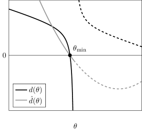
Figure 1: The Parlett-Reid last-pivot function $d(\theta)$ and the lifted function $\hat{d}(\theta)$ have the common zero $\theta_{\min}$. Dashed lines show the analytic continuation of the right hand side of $d(\theta)=\prod_{j}(\theta-\theta_{j})/\prod_{j}(\theta-\hat{\theta}_{j})$ into the region where $d(\theta)=-\infty$.

For sucessive pL iterations, the fact that the tridiagonal matrices grow by one column and row in each iteration may be exploited to save most of the computational effort involved. As noted by Parlett and Reid [41], the reccurence to compute the $d_{i}$ via Cholesky decomposition of $T-\theta I$ in Def. 9 is identical with the recurrence that results from applying a Laplace expansion for the determinant of tridiagonal matrices [18, §2.1.4]. Comparing the recurrences thus yields the explicit formula

$$d(\theta)=\frac{\det(T-\theta I)}{\det(\hat{T}-\theta I)}={-}\frac{\prod_{j}(\theta-\theta_{j})}{\prod_{j}(\theta-\hat{\theta}_{j})},$$ (9)

where $\hat{T}$ denotes the principal submatrix of $T$ obtained by erasing the last column and row, and $\theta_{j}$ and $\hat{\theta}_{j}$ enumerate the eigenvalues of $T$ and $\hat{T}$, respectively. The right hand side is obtained by identifying numerator and denominator with the characteristic polynomials of $T$ and $\hat{T}$, and by factorizing these.

It becomes apparent that $d(\theta)$ has a pole of first order in $\hat{\theta}_{\min}$. After lifting this pole, the function $\hat{d}(\theta):=(\theta-\hat{\theta}_{\min})d(\theta)$ is smooth on a larger interval. When iteratively constructing the tridiagonal matrices in successive pL iterations, the value $\hat{\theta}_{\min}$ is readily available and it becomes preferrable to use $\hat{d}(\theta)$ instead of $d(\theta)$ for root finding.

3.5 Solving the Tridiagonal Subproblem in the Hard Case

If the hard case is present, the decomposition of $T$ into irreducible components has to be determined. This is given in a natural way by Lanczos breakdown. Every time the Lanczos process breaks down and is restarted with a vector $M$-orthogonal to the previously considered Krylov subspaces, a new tridiagonal block is obtained. Solving the problem in the hard case then amounts to applying Theorem 8: First all smallest eigenvalue $\theta_{i}$ of the irreducible blocks $R_{i}$ have to be determined as well as the KKT tuple $(\bm{x_{1}^{*}},\lambda_{1}^{*})$ by solving the easy case for $\text{TR}(R_{1},\gamma^{0}\bm{e_{1}},I,\Delta,\mathbb{R}^{r_{1}})$. Again, let $\ell$ be the smallest index $i$ with minimial $\theta_{i}$. In the case $\lambda_{1}^{*}\geq-\theta_{\ell}$, the global solution is given by $x^{*}=((\bm{x_{1}^{*}})^{T},\ \bm{0},\ \ldots,\bm{0})^{T}$. On the other hand if $\lambda_{1}^{*}<-\theta_{\ell}$ the eigenspace of $R_{\ell}$ corresponding to $\theta_{\ell}$ has to be obtained. As $R_{\ell}$ is irreducible, all eigenvalues of $R_{\ell}$ are simple and an eigenvector $\bm{\tilde{v}}$ spanning the desired eigenspace can be obtained for example by inverse iteration [18, §8.2.2]. The solution is now given by $\bm{x^{*}}=(\bm{x_{1}(-\theta_{\ell})}^{T},\ \bm{0},\ \bm{v}^{T},\ \bm{0})^{T}$ with $\bm{x_{1}}(-\theta_{\min})=(R_{1}-\theta_{\ell}I)^{-1}(-\gamma^{0}\bm{e_{1}})$ and $\bm{v}:=\alpha\bm{\tilde{v}}$ where $\alpha$ has been chosen as the root of the scalar quadratic equation $\Delta^{2}=\|\bm{x_{1}}(-\theta_{\min})\|^{2}+\alpha^{2}\|\bm{\tilde{v}}\|^{2}$ that leads to the smaller objective value.

4 Implementation trlib

In this section, we present details of our implementation trlib of the GLTR method.

4.1 Existing Implementation

The GLTR reference implementation is the software package GLTR in the optimization library GALAHAD [17]. This Fortran 90 implementation uses conjugate gradient iterations exclusively to build up the Krylov subspace, and provides a reverse communication interface that requires exchange vector data to be stored as contiguous arrays in memory.

4.2 trlib Implementation

Our implementation is called trlib, short for trust region library. It is written in plain ANSI C99 code, and has been made available as open source [32]. We provide a reverse communication interface in which only scalar data and requests for vector operations are exchanged, allowing for great flexibility in applications.

Beside the stable and efficient conjugate gradient iteration we also implemented the Lanczos iteration and a crossover mechanism to expand the Krylov subspace, as we frequently found applications in the context of constrained optimization with an SLEQP algorithm [4, 30] where conjugate gradient iterations broke down whenever directions of tiny curvature have been encountered.

4.3 Vector Free Reverse Communication Interface

The implementation is built around a reverse communication calling paradigm. To solve a trust region subproblem, the according library function has to be repeatedly called by the user and after each call the user has to perform a specific action indicated by the value of an output variable. Only scalar data representing dot products and coefficients in axpy operations as well as integer and floating point workspace to hold data for the tridiagonal subproblems is passed between the user and the library. In particular, all vector data has to be managed by the user, who must be able to compute dot products $\langle x,y\rangle$, perform axpy $y:=\alpha x+y$ on them and implement operator vector products $x\mapsto Hx,x\mapsto M^{-1}x$ with the Hessian and the preconditioner.

Thus no assumption about representation and storage of vectorial data is made, as well as no assumption on the discretization of $\mathcal{H}$ if $\mathcal{H}$ is not finite-dimensional. This is beneficial in problems arising from optimization problems stated in function space that may not be stored naturally as contiguous vectors in memory or where adaptivity regarding the discretization may be used along the solution of the trust region subproblem. It also gives a trivial mechanism for exploiting parallelism in vector operations as vector data may be stored and operations may be performed on GPU without any changes in the trust region library.

In particular, this interface allows for easy interfacing with the PDE-constrained optimization software DOLFIN-adjoint [15, 16] within the finite element framework FEniCS [3, 33, 2] without having to rely on assumptions how the finite element discretization is stored, see §5.2.

4.4 Conjugate Gradient Breakdown

Per default, conjugate gradient iterations are used to build the Krylov subspace. The algorithm switches to Lanczos iterations if the magnitude of the curvature $|\langle\hat{p},H\hat{p}\rangle|\leq\emph{{tol\_curvature}}$ with a user defined tolerance $\emph{{tol\_curvature}}\geq 0$.

4.5 Easy Case

In the easy case after the Krylov space has been assembled in a particular iteration it remains to solve $(\textup{TR}(T_{i},\gamma^{0}\bm{e_{1}},I,\Delta,\mathbb{R}^{i+1}))$ which we do as outlined in §3.3. As mentioned there, an improved convergence order can be obtained by higher order Taylor expansions of $\sigma_{p}(\lambda)$ and values $p\neq-1$, see [21]. However in our cases the computational cost for solving the tridiagonal subproblem — often warmstarted in a suitable way — is negligible in comparison the the cost of computing matrix vector products $x\mapsto Hx$ and thus we decided to stick to the simpler Newton rootfinding on $\sigma_{-1}(\lambda)$.

To obtain a suitable initial value $\lambda^{0}$ for the Newton iteration, we first try $\lambda^{*}$ obtained in the previous Krylov iteration if available and otherwise $\lambda^{0}=0$. If these fail, we use $\lambda^{0}=-\theta_{\min}$ computed as outlined in §3.4 by zero-finding on $d(\theta)$ or $\hat{d}(\theta)$. This requires suitable models for $\hat{d}(\theta)$. Gould et al. [19] propose to use a quadratic model $\theta^{2}+a\theta+b$ for $\hat{d}(\theta)$ that captures the asymptotics $t\to-\infty$ obtained by fitting function value and derivative in a point in the root finding process. We have also had good success with the linear Newton model $a\theta+b$, and with using a second order quadratic model $a\theta^{2}+b\theta+c$, that makes use of an additional second derivative, as well. Derivatives of $d(\theta)$ or $\hat{d}(\theta)$ are easily obtained by differentiating the recurrence for the Cholesky decomposition. In our implementation a heuristic is used to select the option that is inside the interval of safety and promises good progress. The heuristic is given by using $\theta^{2}+a\theta+b$ in case that the bracket width $\theta^{k}_{\text{u}}-\theta^{k}_{\ell}$ satisfies $\theta^{k}_{\text{u}}-\theta^{k}_{\ell}\geq 0.1\max\{1,|\theta^{k}|\}$ and $a\theta^{2}+b\theta+c$ otherwise. The motivation behind this is that in the former case it is not guaranteed, that $\theta^{k}$ has been determined to high accuracy as zero of $d(\theta)$ and thus the model that captures the global behaviour might be better suited. In the latter case, $\theta^{k}$ has been confirmed to be a zero of $d(\theta)$ to a certain accuracy and it is safe to use the model representing local behaviour.

4.6 Hard Case

We now discuss the so-called hard case of the trust region problem, which we have found to be of critical importance for the performance of trust region subproblem solvers in general nonlinear nonconvex programming. We discuss algorithmic and numerical choices made in trlib that we have found to help improve performance and stability.

4.6.1 Exact Hard Case

The function for the solution of the tridiagonal subproblem implements the algorithm as given by Theorem 8 if provided with a decomposition in irreducible blocks.

However, from local information it is not possible to distinguish between convergence to a global solution of the original problem and the case in which an invariant Krylov subspace is exhausted that may not contain the global minimizer as in both cases the gradient vanishes.

The handling of the hard case is thus left to the user who has to decide in the reverse calling scheme if once arrived at a point where the gradient norm is sufficiently small the solution in the Krylov subspaces investigated so far or further Krylov subspaces should be investigated. In that case it is left to the user to determine a new nonzero initial vector for the Lanczos iteration that is $M$-orthogonal to the previous Krylov subspaces. One possibility to obtain such a vector is using a random vector and $M$-orthogonalizing it with respect to the previous Lanczos directions using the modified Gram-Schmidt algorithm.

4.6.2 Near Hard Case

The near hard case arises if $\langle\gamma^{0}\bm{e_{1}},\frac{\bm{\tilde{v}}}{\|\bm{\tilde{v}}\|}\rangle$ is tiny, where $\bm{\tilde{v}}$ spans the eigenspace $\text{Eig}(\theta_{\min})=\text{span}\{\bm{\tilde{v}}\}$.

Numerically this is detected if there is no $\lambda\geq\max\{0,-\theta_{\min}\}$ such that $\|\bm{x}(\lambda)\|\geq\Delta$ holds in floating point airthmetic. In that case we use the heuristic $\lambda^{*}=-\theta_{\min}$ and $x^{*}=x(-\theta_{\min})+\alpha\bm{v}$ with $\bm{v}\in\text{Eig}(\theta_{\min})$ where $\alpha$ is determined such that $\|\bm{x^{*}}\|=\Delta$.

Another possibility would be to modify the tridiagonal matrix $T$ by dropping offdiagonal elements below a specified treshold and work on the obtained decomposition into irreducible blocks. However we have not investigated this possibility as the heuristic seems to deliver satisfactory results in practice.

4.7 Reentry with New Trust Region Radius

In nonlinear programming applications it is common that after a rejected step another closely related trust region subproblem has to be solved with the only changed data being the trust region radius. As this has no influence on the Krylov subspace but only on the solution of the tridiagonal subproblem, efficient hotstarting has been implemented. Here the tridiagonal subproblem is solved again with exchanged radius and termination tested. If this point does not satisfy the termination criterion, conjugate gradient or Lanczos iterations are resumed until convergence. However, we rarely observed the need to resume the Krylov iterations in practice.

An explanation is offered based on the use of the convergence criterion

$$\|\nabla L\|_{M^{-1}}\leq\emph{{tol}}$$

as follows: In the Krylov subspace $\mathcal{K}_{i}$,

$$\|\nabla L\|_{M^{-1}}=\gamma^{i+1}|\langle\bm{x}(\lambda),\bm{e_{i+1}}\rangle|\leq\gamma^{i+1}\|\bm{x}(\lambda)\|_{2}=\gamma^{i+1}\Delta.$$

Convergence occurs thus if either $\gamma^{i+1}$ or the last component of $\bm{x}(\lambda)\leq\Delta$ are small. Reducing the trust region radius also reduces the upper bound for $\|\nabla L\|_{M^{-1}}$, so convergence is likely to occur, especially if $\gamma^{i+1}$ turns out to be small.

If the trust region radius is small enough, or equivalently the Lagrange multiplier large enough, it can be proven that a decrease in the trust region radius leads to a decrease in $\|\nabla L\|_{M^{-1}}$:

Lemma 10.

There is $\hat{\lambda}\geq\max_{i}|\lambda_{i}(T)|$ such that $\lambda\mapsto\gamma^{i+1}|\langle\bm{x}(\lambda),\bm{e_{i+1}}\rangle|$ is a decreasing function for $\lambda\geq\hat{\lambda}$.

Proof.

Using the expansion

$$(T_{i}+\lambda I)^{-1}=\sum_{k\geq 0}(-1)^{k}\tfrac{1}{\lambda^{k+1}}T^{k},$$

which holds for $\lambda\geq\max_{i}|\lambda_{i}(T)|$, we find:

$$\|\nabla L\|_{M^{-}1} =\gamma^{i+1}|\langle\bm{x}(\lambda),\bm{e_{i+1}}\rangle|=\gamma^{i+1}\gamma^{0}|\langle(T_{i}+\lambda I)^{-1}\bm{e_{1}},\bm{e_{i+1}}\rangle|$$

$$=\gamma^{i+1}\gamma^{0}\left|\sum_{k\geq 0}(-1)^{k}\tfrac{1}{\lambda^{k+1}}\bm{e_{i+1}}^{T}T^{k}\bm{e_{1}}\right|=\frac{\prod_{j=0}^{i+1}\gamma^{j}}{\lambda^{i+1}}+O((\tfrac{1}{\lambda})^{i+2}),$$

where we have made use of the facts that $\bm{e_{i+1}^{T}}T^{k}\bm{e_{0}}$ vanishes for $k<i$, and that $\bm{e_{i+1}^{T}}T^{k}\bm{e_{0}}=\prod_{j=1}^{i}\gamma^{j}$, which can be easily proved using the relation $T\bm{e_{j}}=\gamma^{j-1}\bm{e_{j-1}}+\gamma^{j+1}\bm{e_{j+1}}+\delta_{j}\bm{e_{j}}$. The claim now holds if $\lambda$ is large enough such that higher order terms in this expansion can be neglected. ∎

4.8 Termination criterion

Convergence is reported as soon as the Lagrangian gradient satisfies

$$\|\nabla L\|_{M^{-1}}\leq\begin{cases}\max\{\emph{{tol\_abs\_i}},\emph{{tol\_rel\_i}}\,\|g\|_{M^{-1}}\},&\text{if }\lambda=0\\ \max\{\emph{{tol\_abs\_b}},\emph{{tol\_rel\_b}}\,\|g\|_{M^{-1}}\},&\text{if }\lambda>0\end{cases}.$$

The rationale for using possibly different tolerances in the interior and boundary case is motivated from applications in nonlinear optimization where trust region subproblems are used as globalization mechanism. There a local minimizer of the nonlinear problem will be an interior solution to the trust region subproblem and it is thus not necessary to solve the trust region subproblem in the boundary case to highest accuracy.

4.9 Heuristic addressing ill-conditioning

The pL directions $P_{i}$ are $M$-orthogonal if computed using exact arithmetic. It is well known that, in finite precision and if $H$ is ill-conditioned, $M$-orthogonality may be lost due to propagation of roundoff errors . An indication that this happened may be had by verifying

$$\tfrac{1}{2}\langle\bm{h},T_{i}\bm{h}\rangle+\gamma^{0}\langle\bm{h},\bm{e_{1}}\rangle=q(P_{i}\bm{h}),$$

which holds if $P_{i}$ indeed is $M$-orthogonal. On several badly scaled instances, for example ARGLINB of the CUTEst test set, we have seen that that both quantities above may even differ in sign, in which case the solution of the trust-region subproblem would yield a direction of ascent. This issue becomes especially severe if $H$ has small, but positive eigenvalues and admits an interior solution of the trust region subproblem. Then, the Ritz values computed as eigenvalues of $T_{i}$ may very well be negative due to the introduction of roundoff errors, and enforce a convergence to a boundary point of the trust region subproblem. Finally, if the trust region radius $\Delta$ is large, the two “solutions” can differ in a significantly.

To address this observation, we have developed a heuristic that, by convexification, permits to obtain a descent direction of progress even if $P_{i}$ has lost $M$-orthogonality. For this, let $\underline{\rho}:=\min_{j}\frac{\langle p_{j},Hp_{j}\rangle}{\langle p_{j},Mp_{j}\rangle}$ and $\overline{\rho}:=\max_{j}\frac{\langle p_{j},Hp_{j}\rangle}{\langle p_{j},Mp_{j}\rangle}$ be the minimal respective and Rayleigh quotients used as estimates of extremal eigenvalues of $H$. Both are cheap to compute during the Krylov subspace iterations.

1. If algorithm 1 has converged with a boundary solution such that $\lambda\geq 10^{-2}\max\{1,\rho_{\max}\}$ and $|\rho_{\min}|\leq 10^{-8}\rho_{\max}$, the case described above may be at hand. We compute $q_{x}:=q(P_{i}\bm{h})$ in addition to $q_{h}:=\tfrac{1}{2}\langle\bm{h},T_{i}\bm{h}\rangle+\gamma^{0}\langle\bm{h},\bm{e_{1}}\rangle$. If either $q_{x}>0$ or $|q_{x}-q_{h}|>10^{-7}\max\{1,|q_{x}|\}$, we resolve with a convexified problem.

2. The convexification heuristic we use is obtained by adding a positive diagonal matrix $D$ to $T_{i}$, where $D$ is chosen such that $T_{i}+D$ is positive definite. We then resolve then the tridiagonal problem with $T_{i}+D$ as the new convexified tridiagonal matrix. We obtain $D$ by attempting to compute a Cholesky factor $T_{i}$. Monitoring the pivots in the Cholesky factorization, we choose $d_{j}$ such that the pivots $\pi_{j}$ are at least slightly positive. The formal procedure is given in algorithm 4. Computational results use the constants $\varepsilon=10^{-12}$ and $\sigma=10$.

input : $T_{i}$, $\varepsilon>0$, $\sigma>0$

output : $D$ such that $T_{i}+D$ is positive definite

for $j=0,\ldots,i$ do

       $\hat{\pi}_{j}:=\begin{cases}\delta_{0},&j=0\\ \delta_{j}-\gamma_{j}^{2}/\pi_{j-1},&j>0\end{cases}$

       $d_{j}:=\begin{cases}0,&\hat{\pi}_{j}\geq\varepsilon\\ \sigma|\gamma_{j}^{2}/\pi_{j-1}-\delta_{j}|,&\hat{\pi}_{j}<\varepsilon\end{cases}$

       $\pi_{j}:=\hat{\pi}_{j}+d_{j}$

      

end for

Algorithm 4 Convexification heuristic for the tridiagonal matrix $T_{i}$.

4.10 TRACE

In the recently proposed TRACE algorithm [10], trust region problems are also used. In addition to solving trust region problems, the following operations have to be performed:

• $\min_{x}\tfrac{1}{2}\langle x,(H+\lambda M)x\rangle+\langle g,x\rangle$,

• Given constants $\sigma_{\text{l}},\sigma_{\text{u}}$ compute $\lambda$ such that the solution point of $\min_{x}\tfrac{1}{2}\langle x,(H+\lambda M)x\rangle+\langle g,x\rangle$ satisfies $\sigma_{\text{l}}\leq\frac{\lambda}{\|x\|_{M}}\leq\sigma_{\text{u}}$.

These operations have to be performed after a trust region problem has been solved and can be efficiently implemented using the Krylov subspaces already built up.

We have implemented these as suggested in [10], where the first operation requires one backsolve with tridiagonal data and the second one is implemented as root finding on $\lambda\mapsto\tfrac{\lambda}{\|x(\lambda)\|}-\sigma$ with a certain $\sigma\in[\sigma_{\text{l}},\sigma_{\text{u}}]$ that is terminated as soon as $\tfrac{\lambda}{\|x(\lambda)\|}\in[\sigma_{\text{l}},\sigma_{\text{u}}]$.

4.11 C11 Interface

The algorithm has been implemented in C11. The user is responsible for holding vector-data and invokes the algorithm by repeated calls to the function trlib_krylov_min with integer and floating point workspace and dot products $\langle v,g\rangle,\langle p,Hp\rangle$ as arguments and in return receives status informations and instructions to be performed on the vectorial data. A detailed reference is provided in the Doxygen documentation to the code.

4.12 Python Interface

A low-level python interface to the C library has been created using Cython that closely resembles the C API and allows for easy integration into more user-friendly, high-level interfaces.

As a particular example, a trust region solver for PDE-constrained optimization problems has been developed to be used from DOLFIN-adjoint [15, 16] within FEniCS [3, 33, 2]. Here vectorial data is only considered as FEniCS-objects and no numerical data except of dot products is used of these objects.

5 Numerical Results

In this section, we present an assessment of the computational performance of our implementation trlib of the GLTR method, and compare it to the reference implementation GLTR as well as several competing methods for solving the trust region problem and their respective implementations.

5.1 Generation of Trust-Region Subproblems

For want of a reference benchmark set of non-convex trust region subproblems, we resorted to the subset of unconstrained nonlinear programming problems of the CUTEst benchmark library, and use a standard trust region algorithm, e.g. Gould et al. [19], for solving $\min_{\bm{x}\in\mathbb{R}^{n}}f(\bm{x})$, as a generator of trust-region subproblems. The algorithm starts from a given initial point $\bm{x^{0}}\in\mathbb{R}^{n}$ and trust region radius $\Delta^{0}>0$, and iterates for $k\geq 0$:

input : $f$, $x^{0}$, $\Delta^{0}$, $\rho_{\textup{acc}}$, $\rho_{\textup{inc}}$, $\gamma^{+}$, $\gamma^{-}$, tol_abs

output : $k$, $x^{k}$

for $k\geq 0$ do

       Evaluate $\bm{g^{k}}:=\nabla f(\bm{x^{k}})$

       Test for termination: Stop if $\|\bm{g^{k}}\|\leq\emph{{tol\_abs}}$

       Evaluate $H^{k}:=\nabla^{2}_{\bm{xx}}f(\bm{x^{k}})$

       Compute (approximate) minimizer $\bm{d^{k}}$ to $\text{TR}(H^{k},\bm{g^{k}},I,\Delta^{k})$

       Assess the performance $\rho^{k}:=({f(\bm{x^{k}}+\bm{d^{k}})-f(\bm{x^{k}})})/{q(\bm{d^{k}})}$ of the step

       Update step: $\bm{x^{k+1}}:=\begin{cases}\bm{x^{k}}+\bm{d^{k}},&\rho^{k}\geq\rho_{\text{acc}}\\ \bm{x^{k}},&\rho^{k}<\rho_{\text{acc}}\end{cases},$

       Update trust region radius: $\Delta^{k+1}:=\begin{cases}\gamma^{+}\Delta^{k},&\rho^{k}\geq\rho_{\text{inc}}\\ \Delta^{k},&\rho_{\text{acc}}\leq\rho^{k}<\rho_{\text{inc}}\\ \gamma^{-}\Delta^{k},&\rho^{k}<\rho_{\text{acc}}\end{cases}$

      

end for

Algorithm 5 Standard trust region algorithm for unconstrained nonlinear programming, used to generate trust region subproblems from CUTEst.

In a first study, we compared our implementation trlib of the GLTR method to the reference implementation GLTR as well as several competing methods for solving the trust region problem, and their respective implementations, as follows:

• GLTR [19] in the GALAHAD library implements the GLTR method.

• LSTRS [47] uses an eigenvalue based approach. The implementation uses MATLAB and makes use of the direct ARPACK [29] reverse communication interface, which is deprecated in recent versions of MATLAB and lead to crashes within MATLAB 2013b used by us. We thus resorted to the standard eigs eigenvalue solver provided by MATLAB which might severly impact the behaviour of the algorithm.

• SSM [22] implements a sequential subspace method that may use an SQP accelerated step.

• ST is an implementation of the truncated conjugate gradient method proposed independently by Steihaug [49] and Toint [50].

• trlib is our implementation of the GLTR method.

All codes, with the exception of LSTRS, have been implemented in a compiled language, Fortran 90 in case of GLTR and C in for all other codes, by their respective authors. LSTRS has been implemented in interpreted MATLAB code. The benchmark code used to run this comparison has also been made open source and is available as trbench [31].

In our test case the parameters $\Delta^{0}=\tfrac{1}{\sqrt{n}}$, $\emph{{tol\_abs}}=10^{-7}$, $\rho_{\text{acc}}=10^{-2}$, $\rho_{\text{inc}}=0.95$, $\gamma^{+}=2$ and $\gamma^{-}=\tfrac{1}{2}$ have been used. We used the subproblem convergence criteria as specified in table 1 for the different solvers, trying to have as comparable convergence criteria as possible within the available applications. Our rationale for the interior convergence criterion to request $\|\nabla L\|_{M^{-1}}=O(\|\bm{g^{k}}\|_{M^{-1}}^{2})$ is that it defines an inexact Newton method with q-quadratic convergence rate, [38, Thm 7.2]. As LSTRS is a method based on solving a generalized eigenvalue problem, its convergence criterion depends on the convergence criterion of the generalized eigensolver and is incomparable with the other termination criteria. With the exception of trlib, no other solver allows to specify different convergence criteria for interior and boundary convergence.

solver	$\tau$ interior convergence	$\tau$ boundary convergence
GLTR	$\min\{0.5,\|\bm{g^{k}}\|_{M^{-1}}\}\|\bm{g^{k}}\|_{M^{-1}}$	identical to interior
LSTRS	defined in dependence of convergence of implicit restarted Arnoldi method
SSM	$\min\{0.5,\|\bm{g^{k}}\|\}_{M^{-1}}\|\bm{g^{k}}\|_{M^{-1}}$	identical to interior
ST	$\min\{0.5,\|\bm{g^{k}}\|\}_{M^{-1}}\|\bm{g^{k}}\|_{M^{-1}}$	method heuristic in that case
trlib	$\min\{0.5,\|\bm{g^{k}}\|\}_{M^{-1}}\|\bm{g^{k}}\|_{M^{-1}}$	$\max\{10^{-6},\min\{0.5,\|\bm{g^{k}}\|_{M^{-1}}^{1/2}\}\}\|\bm{g^{k}}\|_{M^{-1}}$

Table 1: Convergence criteria for subproblem solvers $\|\nabla L\|_{M^{-1}}\leq\tau$

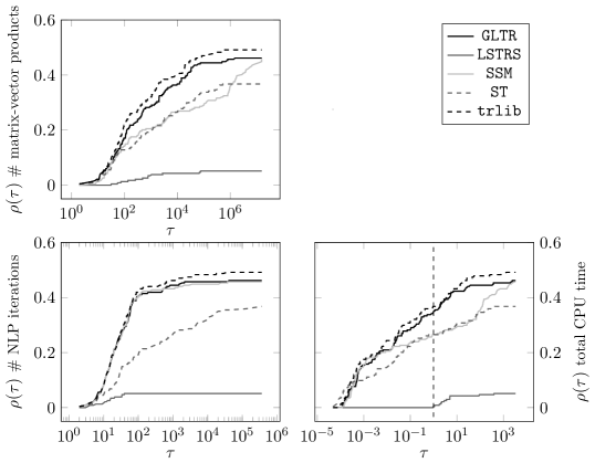
Figure 2: Performance Profiles for matrix-vector products, NLP iterations and total CPU time for different trust region subproblem solvers when used in a standard trust region algorithm for unconstrained minimization evaluated on the set of all unconstrained minimization problems from the CUTEst library.

The performance of the different algorithms is assessed using extended performance profiles as introduced by [12, 34], for a given set $S$ of solvers and $P$ of problems the performance profile for solver $s\in S$ is defined by

$$\rho_{s}(\tau):=\frac{1}{|P|}|\{p\in P\,|\,r_{s,p}\leq\tau\}|,\quad\text{where }r_{s,p}=\frac{t_{s,p}\text{ performance of }s\in S\text{ on }p\in P}{\min_{\sigma\in S,\sigma\neq s}t_{\sigma,p}}.$$

It can be seen that GLTR and trlib are the most robust solvers on the subset of unconstrained problems from CUTEst in the sense that they eventually solve the largest fraction of problems among all solversand that they are also among the fastest solvers. That GLTR and trlib show similar performance is to be expected as they implement the identical GLTR algorithm, where trlib is slightly more robust and faster. We attribute this to the implementation of efficient hotstart capabilities and also the Lanczos process to build up the Krylov subspaces once directions of zero curvature are encountered. Tables 2–4 show the individual results on the CUTEst library.

problem	$n$	GLTR		LSTRS		SSM		ST		trlib
		$\|\nabla f\|$	# $Hv$	$\|\nabla f\|$	# $Hv$	$\|\nabla f\|$	# $Hv$	$\|\nabla f\|$	# $Hv$	$\|\nabla f\|$	# $Hv$
AKIVA	2	3.7e-04	12	1.7e-03	104	3.7e-04	18	3.7e-04	12	3.7e-04	12
ALLINITU	4	1.2e-06	28	1.9e-05	275	1.2e-06	30	3.3e-05	20	1.2e-06	27
ARGLINA	200	2.1e-13	9	1.0e-13	485	2.8e-13	648	1.9e-13	10	1.8e-13	9
ARGLINB	200	1.4e-01	9	2.1e-01	14695	failure		3.6e-04	152	9.7e-03	76
ARGLINC	200	7.9e-02	9	3.1e-01	9177	failure		1.6e-03	156	5.1e-02	21
ARGTRIGLS	10	1.0e-09	50	3.6e-06	372	1.0e-09	15	1.2e-08	42	1.0e-09	50
ARWHEAD	5000	3.7e-11	20	2.4e-08	1054	3.7e-11	551752	3.7e-10	24	3.7e-11	17
BA-L16LS	66462	1.1e+06	58453	9.8e+07	83115	failure		2.4e+06	20698	1.1e+08	21941
BA-L1LS	57	4.6e-08	317	1.3e+01	72289	6.0e-08	30336	1.2e-08	436	2.4e-08	758
BA-L21LS	34134	6.2e+06	129819	5.7e+07	208393	2.7e+09	1123576	1.2e+06	43139	9.8e+05	36639
BA-L49LS	23769	4.4e+04	250639	1.7e+06	1412516	failure		2.9e+05	60741	8.7e+05	35305
BA-L52LS	192627	3.5e+08	21964	6.7e+09	36939	failure		3.1e+07	16589	2.7e+07	19543
BA-L73LS	33753	1.4e+06	161282	7.1e+12	32865	failure		7.5e+11	10071	4.7e+07	92020
BARD	3	5.6e-07	23	failure		5.6e-07	24	9.8e-08	2910	5.6e-07	24
BDQRTIC	5000	5.7e-04	218	5.8e-04	4235	5.7e-04	811903	1.0e-02	529	5.7e-04	209
BEALE	2	1.2e-08	16	4.8e-06	93	1.2e-08	24	2.0e-08	62	1.2e-08	16
BENNETT5LS	3	6.5e-08	405	failure		2.2e-04	2256	9.9e-08	876	1.8e-08	1691
BIGGS6	6	1.8e-08	71	failure		5.9e-09	108	2.5e-04	20128	2.1e-08	410
BOX	10000	4.0e-04	32	6.8e-05	1021	4.0e-04	3278	1.8e-05	2172	4.0e-04	32
BOX3	3	6.6e-11	24	failure		6.6e-11	24	1.0e-07	17266	6.6e-11	24
BOXBODLS	2	2.6e-01	50	7.8e-05	450	2.6e-01	87	3.8e-01	23	2.6e-01	42
BOXPOWER	20000	2.4e-08	86	failure		1.6e+05	10285059	4.7e-05	1335136	5.6e-08	107
BRKMCC	2	6.1e-06	6	2.0e-08	74	6.1e-06	9	6.1e-06	6	6.1e-06	6
BROWNAL	200	2.8e-09	37	failure		4.2e-10	128430	1.0e-07	54218	7.9e-10	32
BROWNBS	2	6.0e-06	75	1.1e-08	777	2.4e-07	99	8.9e-10	69	2.4e-07	67
BROWNDEN	4	7.3e-05	47	5.1e-04	268	7.3e-05	36	1.1e-01	54	7.3e-05	45
BROYDN3DLS	10	6.2e-11	60	4.5e-05	218	6.2e-11	18	1.4e-10	43	6.2e-11	57
BROYDN7D	5000	4.7e-04	13895	1.6e-04	201198	2.9e-04	2285169	1.2e-03	2206	5.8e-04	1660
BROYDNBDLS	10	2.0e-11	110	8.0e-05	466	2.0e-11	33	3.6e-13	70	2.0e-11	105
BRYBND	5000	6.2e-08	630	1.9e-06	93338	1.2e-09	3781397	7.6e-10	733	8.3e-13	639
CHAINWOO	4000	6.6e-04	40920	8.8e+02	69945	1.3e-04	3282530	1.5e-02	41073	3.1e-04	11482
CHNROSNB	50	5.2e-08	2032	8.1e-05	39963	3.5e-09	4008	1.8e-13	629	2.7e-10	1422
CHNRSNBM	50	1.5e-08	3181	1.0e-05	107423	4.4e-08	5065	1.4e-09	809	9.2e-09	1863
CHWIRUT1LS	3	5.4e+00	59	2.3e-01	139	2.1e-01	42	5.3e+00	43	2.1e-01	27
CHWIRUT2LS	3	4.0e-03	57	9.8e-02	138	3.4e-01	39	1.3e-02	37	3.4e-01	23
CLIFF	2	2.1e-05	38	failure		2.1e-05	81	2.1e-05	41	2.1e-05	40
COSINE	10000	1.2e-06	213	7.2e+01	1	1.2e-06	6703	9.3e-03	72	1.2e-06	133
CRAGGLVY	5000	1.3e-04	622	1.2e-04	27113	1.3e-04	4646010	2.3e-03	453	1.3e-04	698
CUBE	2	1.2e-07	64	9.2e-06	564	2.6e-11	105	9.8e-08	204	2.6e-11	50
CURLY10	10000	3.7e-01	93106	1.3e+02	1	3.7e-01	1755070	1.8e-04	290643	4.5e-01	84837
CURLY20	10000	4.2e-03	94429	3.0e+02	1	2.5e-03	1334642	8.3e-02	98598	5.2e-03	96190
CURLY30	10000	2.7e-01	78302	4.2e+03	6974346	2.7e-01	146501	1.9e-02	128689	3.3e-01	77637
DANWOODLS	2	2.2e-06	18	5.6e-06	232	2.2e-06	27	2.2e-06	18	2.2e-06	18
DECONVU	63	2.4e-08	3650	1.3e-03	418777	4.0e-09	37199	2.3e-06	563021	8.3e-08	72328
DENSCHNA	2	6.6e-12	12	5.3e-08	136	6.6e-12	18	6.6e-12	12	6.6e-12	12
DENSCHNB	2	5.8e-10	12	1.3e-06	155	5.8e-10	18	1.0e-10	9	5.8e-10	12
DENSCHNC	2	8.7e-08	20	3.4e-06	237	8.7e-08	30	5.9e-08	20	8.7e-08	20
DENSCHND	3	5.1e-08	114	failure		8.1e-08	135	3.7e-06	11399	8.1e-08	120
DENSCHNE	3	5.2e-12	35	9.5e-05	307	5.2e-12	45	2.1e-10	1442	5.2e-12	25
DENSCHNF	2	2.1e-09	12	3.6e-05	97	2.1e-09	18	1.0e-09	12	2.1e-09	12
DIXMAANA	3000	2.3e-13	44	1.5e-13	2763	2.3e-13	478120	6.7e-21	31	2.3e-13	38
DIXMAANB	3000	5.7e-08	503	7.3e-05	40355	5.7e-08	945986	1.6e-13	37	5.7e-08	80
DIXMAANC	3000	4.5e-12	1382	1.7e-05	40963	4.5e-12	1520049	4.5e-12	37	2.8e-09	95
DIXMAAND	3000	3.4e-13	1533	7.3e-08	68784	3.4e-13	1656761	2.7e-10	38	7.0e-17	169
DIXMAANE	3000	4.6e-08	2012	failure		1.3e-11	3089	4.0e-11	515	1.6e-12	1281
DIXMAANF	3000	4.5e-08	2644	failure		2.1e-08	1348070	1.0e-07	22275	6.7e-11	1079
DIXMAANG	3000	4.8e-08	4035	1.1e+00	845145	1.1e-08	1242789	1.0e-07	22211	2.0e-08	1673
DIXMAANH	3000	3.9e-08	5627	5.5e+02	1950740	5.9e-10	1696337	1.0e-07	22207	8.7e-08	2011
DIXMAANI	3000	1.0e-06	40507	1.0e+03	1	6.1e-06	19337	2.6e-07	3582057	1.8e-12	27353
DIXMAANJ	3000	4.6e-08	23746	2.2e+01	593623	6.2e-13	952725	1.8e-07	3314012	1.7e-07	11321
DIXMAANK	3000	4.6e-08	20831	1.5e+03	3100658	3.3e-11	1555718	1.8e-07	3310116	6.7e-07	14341
DIXMAANL	3000	4.6e-08	24371	3.1e+02	1122879	1.8e-09	1760641	1.8e-07	3319300	1.9e-11	16093
DIXMAANM	3000	4.7e-08	9845	4.4e+02	1	1.4e-11	2559	2.8e-07	4041601	1.0e-05	10745
DIXMAANN	3000	4.7e-08	33134	5.3e-01	1792578	4.5e-09	878377	1.9e-07	3874306	6.1e-08	18948
DIXMAANO	3000	4.8e-08	33105	1.1e-01	1810480	7.4e-08	968909	1.9e-07	3918576	3.4e-09	15832
DIXMAANP	3000	5.4e-08	19509	1.1e+02	90319	2.7e-08	1282847	2.8e-07	5486601	8.5e-10	12074
DIXON3DQ	10000	4.6e-08	40506	5.7e+00	1	6.1e-09	100140	1.3e-05	15308266	1.4e-12	19971
DJTL	2	3.9e+00	155	1.2e+05	1528	1.0e+01	3360	6.6e-01	1029	9.8e+00	2160
DMN15103LS	99	4.2e+01	924732	5.3e+03	177264	1.0e+02	87836914	7.8e+00	783230	6.6e+01	767826
DMN15332LS	66	2.7e-03	719233	8.1e+01	626859	3.6e+01	99777049	2.5e+00	1213511	2.5e+00	996706
DMN15333LS	99	1.5e+01	928176	2.7e+02	730749	failure		5.4e+00	874786	2.9e+00	769091
DMN37142LS	66	9.4e-03	385536	3.1e+01	846259	1.4e-02	63711807	1.7e+00	1256055	1.7e+02	1073546
DMN37143LS	99	1.1e+00	547560	3.5e+03	84848	4.5e+00	41749169	1.4e+01	777991	1.3e+01	736780
DQDRTIC	5000	3.3e-10	39	8.3e-14	792	4.2e-12	3027385	1.3e-11	22	3.2e-10	25
DQRTIC	5000	4.1e-08	14236	1.3e+13	1	3.5e-08	15362086	1.0e-07	369300	3.5e-08	19244
ECKERLE4LS	3	1.8e-08	13	failure		2.4e-08	63	1.6e-07	10001	2.4e-08	57
EDENSCH	2000	5.1e-05	342	9.5e-03	65271	5.1e-05	1645581	1.1e-04	147	5.1e-05	208
EG2	1000	2.9e-08	6	failure		2.1e-04	1126	1.2e-02	11	2.9e-08	6
EIGENALS	2550	4.2e-07	9436	failure		1.9e+00	276726	7.2e-08	151148	3.5e-09	5959
EIGENBLS	2550	6.5e-08	745535	4.8e+00	329779	6.8e-03	475261	3.3e-06	1132767	4.8e-05	1056840

Table 2: Results of subproblem solvers in individual CUTEst problems, part 1

problem	$n$	GLTR		LSTRS		SSM		ST		trlib
		$\|\nabla f\|$	# $Hv$	$\|\nabla f\|$	# $Hv$	$\|\nabla f\|$	# $Hv$	$\|\nabla f\|$	# $Hv$	$\|\nabla f\|$	# $Hv$
EIGENCLS	2652	3.8e-08	796370	failure		5.7e-01	402829	5.4e-09	66267	7.9e-09	270864
ENGVAL1	5000	2.4e-03	120	2.4e-03	18197	2.4e-03	3023116	5.9e-04	96	2.4e-03	107
ENGVAL2	3	6.5e-07	43	5.9e-06	353	4.5e-15	45	0.0e+00	42	1.7e-12	45
ENSOLS	9	9.3e-05	95	9.6e-05	412	9.3e-05	33	2.8e-04	68	9.3e-05	88
ERRINROS	50	7.3e-07	1446	failure		9.0e-04	6582	7.6e-07	109821	9.2e-04	883
ERRINRSM	50	1.1e-03	2817	failure		8.3e-03	5037	2.6e-06	720904	8.3e-03	1487
EXPFIT	2	2.1e-06	17	6.1e-07	131	4.8e-09	24	5.8e-06	17	4.8e-09	12
EXTROSNB	1000	9.9e-08	33028	2.3e-01	18905	5.7e-08	3716226	2.7e-06	12048850	1.0e-07	247139
FBRAIN2LS	4	2.8e-01	236	failure		1.3e-02	138	4.5e-04	30008	1.3e-02	187
FBRAIN3LS	6	1.5e-06	60534	failure		1.6e+01	486095	2.6e-03	39955	8.6e-08	30562
FBRAINLS	2	3.4e-05	14	3.9e-05	149	3.4e-05	21	8.6e-05	14	3.4e-05	14
FLETBV3M	5000	9.1e-03	4883	failure		1.1e-03	19423	2.2e-05	885	2.6e-03	1379
FLETCBV2	5000	failure		failure		failure		failure		failure
FLETCBV3	5000	3.1e+01	14194503	3.8e+01	55869908	3.2e+01	15365644	2.1e+01	4726900	3.0e+01	8099116
FLETCHBV	5000	2.7e+09	38547	3.7e+09	14764569	3.0e+09	35263513	3.6e+09	78	3.0e+09	18992
FLETCHCR	1000	4.2e-08	61120	7.0e-05	663337	4.8e-08	300564	4.2e-09	45367	4.8e-08	47342
FMINSRF2	5625	4.3e-08	12601	3.3e-01	1	6.4e-09	44273	5.1e-06	1931678	1.1e-09	3067
FMINSURF	5625	1.0e-07	8750	3.3e-01	1	5.8e-02	27451	6.8e-08	47015	8.7e-06	4011
FREUROTH	5000	3.9e-01	80	3.9e-01	4042	3.9e-01	6628218	6.0e-03	55	3.9e-01	69
GAUSS1LS	8	4.2e+01	68	1.1e+01	288	4.2e+01	21	1.4e+01	71	4.3e+01	60
GAUSS2LS	8	2.7e-01	79	2.3e-01	293	2.7e-01	24	1.4e+01	77	2.7e-01	70
GBRAINLS	2	1.4e-04	12	1.4e-04	94	1.4e-04	18	1.4e-04	12	1.4e-04	12
GENHUMPS	5000	4.8e-11	1486656	6.0e+03	1	4.7e-11	8692146	8.9e-08	35816	5.0e-12	529592
GENROSE	500	6.7e-04	16490	6.1e-05	309312	2.0e-06	66839	3.4e-05	3639	1.1e-04	8682
GROWTHLS	3	5.4e-03	345	3.2e-02	2027	8.9e-03	294	2.4e-03	4075	5.1e-05	239
GULF	3	4.0e-08	74	failure		6.8e-08	78	5.7e-04	19576	6.8e-08	69
HAHN1LS	7	1.8e+03	9794	7.5e+01	5273	8.3e+01	332983	5.1e-01	5459	2.8e+00	592
HAIRY	2	1.7e-04	118	2.5e-05	993	1.2e-03	210	1.6e-03	137	1.2e-03	100
HATFLDD	3	2.1e-08	71	failure		1.5e-11	75	1.0e-07	14033	1.5e-11	69
HATFLDE	3	3.5e-08	54	failure		1.7e-10	57	9.8e-08	3318	1.7e-10	51
HATFLDFL	3	4.7e-08	283	failure		6.6e-08	4404	5.1e-06	28015	3.5e-09	1078
HEART6LS	6	3.5e-08	6521	4.0e+00	29124	5.2e-08	3871	3.3e+00	39973	5.2e-08	8285
HEART8LS	8	4.0e-10	524	1.8e-05	1466	1.9e-09	147	2.0e-13	353	1.9e-09	379
HELIX	3	1.7e-11	36	3.4e-05	330	1.7e-11	36	3.7e-12	32	1.7e-11	36
HIELOW	3	5.4e-03	12	6.7e-03	87	5.4e-03	12	3.2e-05	18	5.4e-03	12
HILBERTA	2	2.8e-15	6	5.4e-15	56	2.2e-16	9	9.5e-08	301	6.2e-15	6
HILBERTB	10	2.4e-09	17	3.0e-06	202	2.4e-14	15	6.3e-10	12	2.4e-09	13
HIMMELBB	2	7.0e-07	18	failure		2.1e-13	75	8.2e-13	33	1.2e-12	19
HIMMELBF	4	4.6e-05	308	failure		4.6e-05	192	1.6e-02	29526	4.6e-05	287
HIMMELBG	2	8.6e-09	8	3.0e-05	62	8.6e-09	12	1.0e-13	11	8.6e-09	8
HIMMELBH	2	5.5e-06	8	7.7e-06	67	5.5e-06	15	5.0e-09	6	5.5e-06	9
HUMPS	2	1.0e-12	2955	4.7e-02	39232	3.1e-11	10767	1.0e-07	2297	2.6e-12	6202
HYDC20LS	99	1.1e-03	97095959	1.9e+06	738933	failure		1.3e-01	93133732	1.3e-01	96002204
INDEF	5000	7.1e+01	297	failure		7.1e+01	28565674	9.1e+01	6895561	7.1e+01	338
INDEFM	100000	1.1e-08	134	failure		failure		1.2e-02	3308	4.6e-09	92
INTEQNELS	12	2.3e-09	12	1.3e-05	145	4.9e-11	9	4.9e-11	15	4.9e-11	15
JENSMP	2	3.4e-02	18	3.4e-02	213	3.4e-02	27	3.4e-02	18	3.4e-02	18
JIMACK	3549	1.1e-04	103654	1.4e+00	1	9.4e-06	123549	9.1e-08	397707	8.8e-05	105680
KIRBY2LS	5	9.5e-03	198	5.1e+01	349	2.5e+00	60	4.2e+00	769	2.7e+00	83
KOWOSB	4	2.3e-07	40	failure		1.0e-07	36	9.9e-08	8576	1.0e-07	40
KOWOSBNE	4	7.0e-08	124	failure		failure		1.0e-07	8375	2.4e-08	68
LANCZOS1LS	6	3.9e-08	484	failure		5.2e-08	348	2.6e-05	29889	7.6e-08	651
LANCZOS2LS	6	3.7e-08	461	1.3e+02	1	1.5e-09	342	2.7e-05	29858	9.6e-08	625
LANCZOS3LS	6	4.1e-08	455	failure		9.9e-08	393	2.6e-05	29950	2.6e-09	757
LIARWHD	5000	1.9e-08	44	3.9e-06	5072	1.9e-08	6202073	3.2e-14	168	1.9e-08	43
LOGHAIRY	2	9.2e-07	5102	failure		8.1e-05	15966	1.5e-03	10003	1.5e-06	6676
LSC1LS	3	2.4e-07	74	1.2e-05	893	2.4e-07	81	5.7e-08	3057	2.4e-07	58
LSC2LS	3	2.2e-05	113	failure		5.1e-05	156	3.8e-02	19975	9.1e-09	162
LUKSAN11LS	100	3.1e-12	14138	1.9e-07	103185	1.8e-12	800008	2.9e-13	2684	1.8e-12	9341
LUKSAN12LS	98	9.2e-03	675	3.7e-02	59360	9.2e-03	2545	1.5e-02	411	9.1e-03	402
LUKSAN13LS	98	5.5e-02	324	1.8e-02	6656	5.5e-02	18870	7.7e-04	176	5.7e-02	237
LUKSAN14LS	98	1.2e-03	580	1.3e-03	47362	1.2e-03	5703	4.2e-06	289	1.2e-03	349
LUKSAN15LS	100	4.7e-03	868	1.4e+00	559146	8.8e-04	4816	9.7e-08	1217	4.0e-04	758
LUKSAN16LS	100	1.2e-05	118	3.0e+04	1	1.2e-05	1229	9.2e-03	91	1.2e-05	123
LUKSAN17LS	100	4.9e-06	1043	1.5e-01	1653079	4.9e-06	6687	2.9e-05	1379	4.9e-06	1208
LUKSAN21LS	100	4.4e-08	2042	2.8e+00	1	7.7e-09	5922	3.3e-08	6962	7.3e-10	1750
LUKSAN22LS	100	7.5e-06	1122	1.5e-04	49915	3.6e-05	1456	1.8e-06	1251618	3.6e-05	893
MANCINO	100	3.4e-05	192	8.3e-05	5269	1.2e-07	206932	1.0e-07	45	1.1e-07	138
MARATOSB	2	9.8e-03	2639	8.7e+00	731	4.8e-02	3006	2.2e-02	1566	4.8e-02	1322
MEXHAT	2	2.0e-05	145	8.7e+01	753	6.6e-04	96	4.3e-04	60	6.6e-04	54
MEYER3	3	1.6e-03	1242	2.3e-03	7573	1.1e+03	933	4.1e-05	3780	8.9e-04	879
MGH09LS	4	1.7e-09	571	failure		6.5e-10	369	6.5e-04	11810	2.1e-07	400
MGH10LS	3	7.2e+03	987	3.3e+06	140325	4.6e+05	552	7.4e+26	751	9.8e+03	193
MGH17LS	5	1.6e+00	41696	failure		9.2e-06	4299	4.9e-06	39945	3.2e-05	772
MISRA1ALS	2	5.4e-04	89	2.4e-04	669	8.2e-02	297	1.3e-05	20002	3.5e-03	74
MISRA1BLS	2	1.1e-01	51	7.9e-02	481	3.0e-04	54	2.1e-04	20002	1.1e-01	50
MISRA1CLS	2	5.0e+00	44	3.2e-04	417	4.5e-04	48	2.4e-02	20002	5.0e+00	43
MISRA1DLS	2	1.3e+00	33	5.1e-03	271	3.1e-02	36	2.7e-03	20002	1.3e+00	32
MODBEALE	20000	4.3e-08	315	7.4e-05	419667	3.1e+05	10995895	6.6e-09	283	2.7e-11	385
MOREBV	5000	4.7e-08	4430	8.0e-04	1	7.4e-09	1126	1.6e-08	50000	1.6e-08	50001

Table 3: Results of subproblem solvers in individual CUTEst problems, part 2

problem	$n$	GLTR		LSTRS		SSM		ST		trlib
		$\|\nabla f\|$	# $Hv$	$\|\nabla f\|$	# $Hv$	$\|\nabla f\|$	# $Hv$	$\|\nabla f\|$	# $Hv$	$\|\nabla f\|$	# $Hv$
MSQRTALS	1024	4.6e-08	31351	1.0e+00	482955	8.7e-09	121693	6.4e-08	71336	7.6e-09	27636
MSQRTBLS	1024	4.7e-08	27153	9.4e-01	430163	6.4e-08	70400	6.9e-08	27457	1.1e-09	18431
NCB20	5010	1.2e-05	17788	2.8e+02	1	1.9e-08	144786	5.0e-06	45317	7.4e-04	5662
NCB20B	5000	4.3e-04	5964	2.8e+02	1	4.3e-04	42004	6.9e-04	4176	4.3e-04	3683
NELSONLS	3	4.5e+04	514	1.6e+05	55911	3.2e+04	1233	1.6e-03	560	2.4e+10	578
NONCVXU2	5000	7.3e-06	128020	3.2e+01	2607687	8.9e-06	8819837	1.3e-05	2616658	2.2e-04	41606
NONCVXUN	5000	1.4e-03	3407516	2.6e+01	2438251	1.5e-02	46939994	5.0e-03	3275980	2.3e-04	3292214
NONDIA	5000	4.6e-09	23	4.9e-07	1188	2.4e-09	5286524	6.1e-08	217	2.2e-09	19
NONDQUAR	5000	8.4e-08	44199	2.0e+04	1	1.9e-08	292931	4.1e-07	10001858	9.6e-08	148134
NONMSQRT	4900	8.3e+01	648705	2.7e+03	285111	3.3e+02	9434595	1.7e+00	604897	3.8e+02	590884
OSBORNEA	5	4.1e-08	220	1.1e-01	979	6.9e-06	126	2.6e-05	49955	6.9e-06	181
OSBORNEB	11	3.5e-07	409	9.4e-05	1570	7.2e-09	90	9.0e-08	4300	7.2e-09	314
OSCIGRAD	100000	6.2e-06	367	3.8e+05	1356648	failure		6.6e-08	205	6.8e-08	380
OSCIPATH	10	2.5e-03	314	1.0e+00	1220	2.0e-02	7596	2.8e-04	80024	1.8e-02	65900
PALMER1C	8	3.8e-08	112	failure		5.5e-08	1484	8.7e+00	78722	4.5e-08	91
PALMER1D	7	3.2e-08	70	failure		2.3e-08	154	9.9e-07	34028	2.5e-08	63
PALMER2C	8	1.3e-08	83	failure		1.5e-08	147	3.8e-03	69856	6.8e-09	71
PALMER3C	8	2.5e-09	84	failure		5.8e-09	27	6.1e-03	69785	1.2e-09	73
PALMER4C	8	1.4e-08	96	failure		8.8e-09	30	1.9e-02	69905	2.9e-09	89
PALMER5C	6	8.2e-14	39	6.3e-14	259	8.2e-14	24	8.3e-14	21	8.3e-14	31
PALMER6C	8	1.0e-08	92	failure		4.6e-09	30	3.2e-01	58799	4.8e-09	79
PALMER7C	8	4.9e-08	121	failure		4.5e-09	52	1.9e-02	59657	3.8e-08	109
PALMER8C	8	1.2e-09	111	failure		3.5e-09	33	2.6e-01	58896	1.1e-09	97
PARKCH	15	4.5e-04	376	7.0e-02	1336	1.8e-04	63	6.6e-02	221	1.8e-04	287
PENALTY1	1000	2.3e-06	90	failure		1.7e+13	2270123	1.0e-07	10284	2.9e-07	84
PENALTY2	200	1.2e+05	326	1.2e+05	8545	1.2e+05	61148	1.4e+02	169	1.2e+05	315
PENALTY3	200	2.5e-06	385	failure		5.3e-08	101235	1.1e-07	1064	9.4e-08	762
POWELLBSLS	2	9.9e-08	162	failure		6.3e-07	378	4.0e-04	20003	8.7e-08	139
POWELLSG	5000	9.9e-08	121	failure		9.4e-08	816877	1.0e-07	381911	9.4e-08	136
POWER	10000	4.9e-08	12229	1.2e+14	30489	failure		1.0e-07	13952	4.5e-08	16380
QUARTC	5000	4.1e-08	14236	1.3e+13	1	3.5e-08	15362086	1.0e-07	369300	3.5e-08	19244
RAT42LS	3	2.1e-01	81	1.3e-04	376	7.1e-05	66	1.6e-04	82	7.0e-05	56
RAT43LS	4	3.1e-01	143	1.1e+00	1098	3.1e-01	99	1.1e-01	428	3.1e-01	106
ROSENBR	2	9.3e-09	45	4.7e-06	521	3.9e-12	78	5.7e-11	46	3.9e-12	42
ROSZMAN1LS	4	9.3e-08	3380	failure		1.1e-04	618	2.0e-04	29991	4.0e-06	114
S308	2	3.7e-06	18	6.4e-06	152	3.7e-06	27	1.8e-07	17	3.7e-06	18
SBRYBND	5000	1.3e+06	646854	2.6e+08	1	6.5e-08	15134337	9.7e+05	8066984	5.5e+03	411061
SCHMVETT	5000	2.2e-04	198	2.4e-04	5965	2.2e-04	2490	6.4e-03	175	2.2e-04	170
SCOSINE	5000	7.3e+02	9514524	3.3e+06	897980	9.7e-02	12118328	1.3e+05	22909922	7.9e+02	769553
SCURLY10	10000	1.7e+04	8358170	4.0e+07	1816763	3.7e+06	13209268	5.5e+05	10383078	9.0e+05	1175003
SCURLY20	10000	9.3e+04	5264236	7.9e+07	1762766	7.0e+06	9436240	2.7e+06	6338695	5.4e+05	1153609
SCURLY30	10000	2.5e+05	3928297	5.5e+07	1696073	1.0e+07	7548932	2.8e+06	4645780	1.2e+06	1087564
SENSORS	100	1.4e-04	351	1.4e-04	20908	1.4e-04	1207	1.6e-04	74	1.3e-04	226
SINEVAL	2	1.7e-07	101	2.0e-06	892	4.2e-17	174	5.4e-08	257	4.3e-17	81
SINQUAD	5000	5.4e+00	68	1.4e-01	6325	5.4e+00	481230	2.4e-02	38	5.4e+00	59
SISSER	2	4.3e-08	28	6.3e-05	229	4.3e-08	48	1.9e-07	10009	4.3e-08	32
SNAIL	2	5.0e-10	161	2.6e-05	1525	5.0e-10	297	2.6e-08	1232	5.0e-10	126
SPARSINE	5000	4.7e-08	490794	8.0e+02	724370	7.4e-09	11750907	3.3e-12	524818	1.4e-11	508898
SPARSQUR	10000	5.3e-08	937	failure		4.5e-08	4741240	1.0e-07	20720	4.6e-08	1309
SPMSRTLS	4999	4.8e-08	2035	9.0e-05	160194	1.3e-08	5368	9.6e-12	4803	8.7e-14	1587
SROSENBR	5000	4.9e-12	28	9.6e-05	13105	4.9e-12	3503	9.2e-08	126	4.9e-12	28
SSBRYBND	5000	4.7e-08	74324	2.4e+06	244155	5.9e-09	5712	3.6e-08	252195	6.1e-10	83610
SSCOSINE	5000	3.9e+02	4072572	5.9e+03	1	1.5e+02	46643	1.7e-01	13991974	2.3e+02	11185306
SSI	3	4.7e-08	1692	failure		8.8e-03	30003	2.2e-04	19968	3.1e-09	2919
STRATEC	10	4.2e-03	381	5.1e-01	1295	4.2e-03	78	3.3e-01	704	4.2e-03	291
TESTQUAD	5000	3.9e-08	2104	4.4e+07	1	1.8e-10	6723210	2.2e-13	3304	3.7e-10	2398
THURBERLS	7	4.2e-01	287	1.4e-01	1392	4.2e-01	2171	8.0e-03	1252	4.1e-01	203
TOINTGOR	50	2.7e-04	348	7.8e-05	30012	2.7e-04	990	6.0e-04	225	2.7e-04	351
TOINTGSS	5000	4.2e-08	148	3.0e-05	3827	4.2e-08	3893828	3.0e-05	147	3.2e-08	82
TOINTPSP	50	9.8e-06	450	8.0e-05	7546	4.5e-03	2842	7.5e-04	211	4.5e-03	248
TOINTQOR	50	4.0e-07	79	9.9e-05	2976	1.6e-09	458	4.9e-08	46	3.8e-07	88
TQUARTIC	5000	2.5e-07	32	6.4e-07	864	2.1e-14	2626	1.0e-07	83144	0.0e+00	35
TRIDIA	5000	4.7e-08	1064	9.8e-05	328271	2.5e-09	1070690	4.2e-14	1425	9.3e-12	1434
VARDIM	200	2.2e-09	33	8.5e-05	38751	9.5e-09	925519	1.7e-09	50	2.6e-09	33
VAREIGVL	50	3.8e-08	436	2.9e-07	13815	1.4e-10	2761	4.0e-08	425	7.7e-09	457
VESUVIALS	8	1.1e-02	821	4.2e+06	974	1.9e-02	11806	2.3e+02	69599	1.7e+01	802
VESUVIOLS	8	1.2e+01	382	1.5e+08	1	3.9e+02	3168	2.7e-01	11149	3.9e+02	187
VESUVIOULS	8	4.7e-03	157	2.4e+04	1417	9.7e-05	685	3.3e-02	131206	4.1e-03	237
VIBRBEAM	8	4.3e-04	465	4.5e+00	2609	2.0e-02	12818	3.7e-04	4213	1.2e-01	336
WATSON	12	4.7e-08	369	failure		6.9e-09	57	1.8e-06	71328	9.4e-08	314
WOODS	4000	3.2e-12	250	6.1e+02	596298	1.4e-12	2771525	1.1e-10	317	1.4e-12	266
YATP1LS	2600	1.2e-09	59	8.1e-09	75319	8.6e-10	873596	1.0e-10	57	1.2e-09	52
YATP2LS	2600	5.7e-01	6160859	4.1e+02	5486629	1.1e+00	2139765	1.3e-10	35	4.4e-03	163257
YFITU	3	1.2e-05	166	failure		4.7e-09	147	3.9e-03	29960	4.7e-09	137
ZANGWIL2	2	0.0e+00	2	1.9e-15	32	0.0e+00	6	0.0e+00	2	0.0e+00	2

Table 4: Results of subproblem solvers in individual CUTEst problems, part 3

5.2 Function Space Problem

We solved a modified variant of SCDIST1 [7, 35] of the OPTPDE benchmark library [39, 40] for PDE constrained optimal control problems. The state constraint has been dropped and a trust region constraint added in order to obtain the following function space trust region problem:

$$\min_{y\in H^{1}(\Omega),u\in L^{2}(\Omega)}\quad \tfrac{1}{2}\|y-y_{\text{d}}\|_{L^{2}(\Omega)}^{2}+\tfrac{\beta}{2}\|u-u_{\text{d}}\|_{L^{2}(\Omega)}^{2}$$

  s.t. $$-\triangle y+y =u, x\in\Omega$$

$$\partial_{n}y =0, x\in\partial\Omega$$

$$\|y\|_{L^{2}(\Omega)}^{2}+\|u\|_{L^{2}(\Omega)}^{2} \leq\Delta^{2}$$

Here $\Omega\subseteq\mathbb{R}^{n}$, $L^{2}(\Omega)$ denotes the Lebesgue space of square integrable functions $f:\Omega\to\mathbb{R}$, $H^{1}(\Omega)$ the sobolev space of square integrable functions that admit a square integrable weak derivative and $\triangle:H$ is the Laplace operator $\triangle=\sum_{i=1}^{n}\partial^{2}_{ii}$.

Tracking data $y_{\text{d}},u_{\text{d}}$ has been used as specified in OPTPDE where typical regularization parameters have been considered in the range $10^{-8}\leq\beta\leq 10^{-3}$. Different geometries $\Omega\in\{(0,1)^{2},(0,1)^{3},\{x\in\mathbb{R}^{2}\,|\,\|x\|\leq 1\},\{x\in\mathbb{R}^{3}\,|\,\|x\|\leq 1\}\}$ have been studied.

The finite element software FEnICS has been used to obtain a finite element discretization of the problem:

$$\min_{\bm{y}\in\mathbb{R}^{n_{y}},\bm{u}\in\mathbb{R}^{n_{u}}}\quad \tfrac{1}{2}\|\bm{y}-\bm{y}_{\text{d}}\|_{M}^{2}+\tfrac{\beta}{2}\|\bm{u}-\bm{u}_{\text{d}}\|_{M}^{2}$$

  s.t. $$A\bm{y}-M\bm{u} =0,$$

$$\|\bm{y}\|_{M}^{2}+\|\bm{u}\|_{M}^{2} \leq\Delta^{2},$$

where $M$ denotes the mass matrix and $A=K+M$ with $K$ being the stiffness matrix.

We used the approach suggested by Gould et al. [20] to solve this equality constrained trust region problem:

1. A null-space projection in the precondioning step of the Krylov subspace iteration is used to satisfy the discretized PDE constraint. The required preconditioner is given by

   $$\begin{pmatrix}\bm{y}\\ \bm{u}\end{pmatrix}\mapsto\begin{pmatrix}I&0&0\\ 0&I&0\end{pmatrix}\begin{pmatrix}M&0&A\\ 0&M&-M\\ A&-M&0\end{pmatrix}^{-1}\begin{pmatrix}I&0\\ 0&I\\ 0&0\end{pmatrix}\begin{pmatrix}\bm{y}\\ \bm{u}\end{pmatrix}.$$

2. We used MINRES [42] for solving with the linear system arising in this preconditioner to high accuracy. MINRES iterations themselves are preconditioned using the approximate Schur-complement preconditioner

   $$\begin{pmatrix}\tilde{M}&&\\ &\tilde{M}&\\ &&\tilde{A}M^{-1}\tilde{A}\end{pmatrix}^{-1},$$

   as proposed by [43]. This preconditioner is an approximation to the optimal preconditioner

   $$\begin{pmatrix}M&&\\ &M&\\ &&AM^{-1}A+M\end{pmatrix}^{-1}$$

   that would lead to mesh-independent MINRES convergence in three iterations, provided exact arithmetic [28, 37] would be used.

3. In the MINRES preconditioner of step (2), products with $\tilde{M}^{-1}$ and $\tilde{A}^{-1}$ are computed using truncated conjugate gradients (CG) to high accuracy, again preconditioned using an algebraic multigrid as preconditioner.

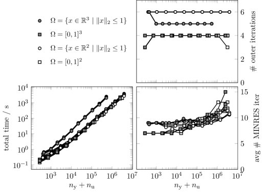
Figure 3: Results for distributed control trust region problem for different mesh sizes. Results are shown for four different geometries. Regularization parameters $\beta\in\{10^{-3},10^{-4},10^{-5},10^{-6},10^{-7},10^{-8}\}$ have been considered, however computational results for a fixed geometry hardly change with $\beta$ leading to near-identical plots.

In Fig. 3, it can be seen that using the GLTR method for these function space problems yields a solver with mesh-independent convergence behavior. The number of outer iterations is virtually constant on a wide range of different meshes and varies at most by one iteration. The number of inner (MINRES) iterations varies only slightly, as is to be expected due to the use of an approximately optimal preconditioner in step (2).

6 Conclusion

We presented trlib which implements Gould’s Generalized Lanczos Method for trust region problems. Distinct features of the implementation are by the choice of a reverse communication interface that does not need access to vector data but only to dot products between vectors and by the implementation of preconditioned Lanczos iterations to build up the Krylov subspace. The package trbench, which relies on CUTEst, has been introduced as a test bench for trust region problem solvers. Our implementation trlib shows similar and favorable performance in comparison to the GLTR implementation of the Generalized Lanczos Method and also in comparison to other iterative methods for solving the trust region problem.

Moreover, we solved an example from PDE constrained optimization to show that the implementation can be used for problems stated in Hilbert space as a function space solver with almost discretization independent behaviour in that example.

Funding

F. Lenders acknowledges funding by the German National Academic Foundation. F. Lenders and C. Kirches acknowledge funding by DFG Graduate School 220, funded by the German Excellence Initiative. C. Kirches acknowledges financial support by the European Union within the 7^th Framework Programme under Grant Agreement n^o 611909 and by Deutsche Forschungsgemeinschaft through Priority Programme 1962 “Non-smooth and Complementarity-based Distributed Parameter Systems: Simulation and Hierarchical Optimization”. C. Kirches and A. Potschka acknowledge funding by the German Federal Ministry of Education and Research program “Mathematics for Innovations in Industry and Service”, grants n^o 05M2013-GOSSIP and 05M2016-MoPhaPro. A. Potschka acknowledges funding by the European Research Council Adv. Inv. Grant MOBOCON 291 458. We are grateful to two anonymous referees who helped to significantly improve the exposition of this article and would like to thank R. Herzog for bibliographic pointers regarding Krylov subspace methods in Hilbert space.

References

- [1] Absil, P.-A., Baker, C., Gallivan, K.: Trust-Region Methods on Riemannian Manifolds. Foundations of Computational Mathematics 7(3), 303–330 (2007)
- [2] Alnæs, M., Logg, A., Ølgaard, K., Rognes, M., Wells, G.: Unified Form Language: A domain-specific language for weak formulations of partial differential equations. ACM Transactions on Mathematical Software 40(2) (2014)
- [3] Alnæs, M., Blechta, J., Hake, J., Johansson, A., Kehlet, B., Logg, A., Richardson, C., Ring, J., Rognes, M., Wells, G.: The FEniCS Project Version 1.5. Archive of Numerical Software, 3(100) (2015)
- [4] Byrd, R., Gould, N., Nocedal, J., Waltz, R.: An algorithm for nonlinear optimization using linear programming and equality constrained subproblems. Mathematical Programming 100(1), 27–48 (2003)
- [5] Cartis, C., Gould, N., Toint, P.: Adaptive cubic regularisation methdos for unconstrained optimization. Part I: motivation, convergence and numerical results. Mathematical Programming 127, 245–295 (2011)
- [6] Cartis, C., Gould, N., Toint, P.: Adaptive cubic regularisation methdos for unconstrained optimization. Part II: worst-case function- and derivative-evaluation complexity Mathematical Programming 130, 295–319 (2011)
- [7] Casas, E.: Control of an elliptic problem with pointwise state constraints. SIAM Journal on Control and Optimization 24(6), 1309–1318 (1986)
- [8] Clarke, F.: Functional Analysis, Calculus of Variations and Optimal Control. Springer (2013)
- [9] Conn, A., Gould, N., Toint, P.: Trust-Region Methods. SIAM (2000)
- [10] Curtis, F., Robinson, D., Samadi, M.: A trust region algorithm with a worst-case iteration complexity of for nonconvex optimization. Mathematical Programming 1–32 (2016)
- [11] Gould, N., Orban, D., Toint, P.: CUTEst: a constrained and unconstrained testing environment with safe threads. Tech. Rep. RAL-TR-2013-005 (2013)
- [12] Dolan, E., Moré, J.: Benchmarking optimization software with performance profiles. Mathematical Programming 91(2), 201–213 (2002)
- [13] Erway, J., Gill, P., Griffin, J.: Iterative Methods for Finding a Trust-region Step. SIAM Journal on Optimization 20(2), 1110–1131 (2009)
- [14] Erway, J., Gill, P.: A Subspace Minimization Method for the Trust-Region Step. SIAM Journal on Optimization 20(3), 1439–1461 (2010)
- [15] Farrell, P., Ham, D., Funke, S., Rognes, M.: Automated derivation of the adjoint of high-level transient finite element programs. SIAM Journal on Scientific Computing 35(4), 369–393 (2013)
- [16] Funke, P., Farrell, P.: A framework for automated PDE-constrained optimisation. preprint arXiv:1302.3894
- [17] Gould, N., Orban, D., Toint, P.: GALAHAD, a library of thread-safe Fortran 90 packages for large-scale nonlinear optimization. ACM Transactions on Mathematical Software 29(4), 353–372 (2004)
- [18] Golub, G., Van Loan, C.: Matrix Computations, Third Edition. John Hopkins University Press (1996)
- [19] Gould, N., Lucidi, S., Roma, M., Toint, P.: Solving the Trust-Region Subproblem using the Lanczos Method. SIAM Journal on Optimization 9(2), 504–525 (1999)
- [20] Gould, N., Hribar, M., Nocedal, J.: On the solution of equality constrained quadratic programming problems arising in optimization. SIAM Journal on Scientific Computing 23, 1376–1395 (2001)
- [21] Gould, N., Robinson, D., Thorne, H.: On solving trust-region and other regularised subproblems in optimization. Mathematical Programming Computation 1, 21–57 (2010)
- [22] Hager, W.: Minimizing a Quadratic over a Sphere. SIAM Journal on Optimization 12(1), 188–208 (2001)
- [23] Heinkenschloss, M.: Mesh independence for nonlinear least squares problems with norm constraints. SIAM Journal on Optimization, 3(1), 81–117 (1993)
- [24] Günnel, A., Herzog, R., Sachs, E.: A note on preconditioners and scalar products in Krylov subspace methods for self-adjoint problems in Hilbert space. Electronic Transactions on Numerical Analysis 41, 13–20 (2014)
- [25] Hestenes, M.: Applications of the theory of quadratic forms in Hilbert space to the calculus of variations. Pacific Journal of Mathematics 4, 525–581 (1951)
- [26] Kelley, C., Sachs, E.: Quasi-Newton methods and unconstrained optimal control problems. SIAM Journal on Control and Optimization, 25(6), 1503–1517 (1987)
- [27] Kurdila, A., Zabarankin, M.: Convex Functional Analysis. Springer (2005)
- [28] Kuznetsov, Y.: Efficient iterative solvers for elliptic finite element problems on nonmatching grids. Russian Journal of Numerical Analysis and Mathematical Modelling 10, 187–211 (1995)
- [29] Lehoucq, R., Sorensen, D., Yang, C.: ARPACK Users’ Guide: Solution of Large-scale Eigenvalue Problems with Implicitly Restarted Arnoldi Methods. SIAM (1998)
- [30] Lenders, F., Kirches, C., Bock. H.: pySLEQP A Sequential Linear Quadratic Programming Method Implemented in Python. In: Modeling, Simulation and Optimization of Complex Processes HPSC 2015, Springer, to appear
- [31] Lenders, F.: trbench. https://github.com/felixlen/trbench
- [32] Lenders, F.: trlib. https://github.com/felixlen/trlib
- [33] Logg, A., Wells, G.: DOLFIN: Automated Finite Element Computing. ACM Transactions on Mathematical Software 37(2) (2010)
- [34] Mahajan, A., Leyffer, S., Kirches, C.: Solving mixed-integer nonlinear programs by QP diving. Technical Report ANL/MCS-P2071-0312, Mathematics and Computer Science Division, Argonne National Laboratory, 9700 South Cass Avenue, Argonne, IL 60439, U.S.A. (2011)
- [35] Meyer, C., Rösch, A., Tröltzsch, F.: Optimal control of PDEs with regularized pointwise state constraints. Computational Optimization and Applications, 33(2–3), 209–228 (2005)
- [36] Moré, J., Sorensen, D.: Computing a Trust Region Step. SIAM Journal on Scientific and Statistical Computing 4, 553–572 (1983)
- [37] Murphy, M., Golub, G., Wathen, A.: A note on preconditioning for indefinite linear systems SIAM Journal on Scientific Computing 21(6), 1969–1972 (1999)
- [38] Nocedal, J., Wright, S.: Numerical Optimization. Springer, 2006.
- [39] Herzog, R., Rösch, A., Ulbrich, S., Wollner, W.: OPTPDE — A Collection of Problems in PDE-Constrained Optimization. http://www.optpde.net
- [40] Herzog, R., Rösch, A., Ulbrich, S., Wollner, W.: OPTPDE — A Collection of Problems in PDE-Constrained Optimization. In: Leugering, G., Benner, P., Engell, S., Griewank, A., Harbrecht, H., Hinze, M., Rannacher, R., Ulbrich, S.: Trends in PDE Constrained Optimization. International Series of Numerical Mathematics 165, 539–543, Springer (2014)
- [41] Parlett, B., Reid, J.: Tracking the Progress of the Lanczos Algorithm for Large Symmetric Eigenproblems. IMA Journal of Numerical Analysis 1, 135–155 (1981)
- [42] Paige, C., Saunders, M.: Solution of sparse indefinite systems of linear equations. SIAM Journal on Numerical Analysis 12(4), 617–629 (1975)
- [43] Rees, T., Dollar, S., Wathen, A.: Optimal Solvers for PDE-Constrained Optimization. SIAM Journal on Scientific Computing 32(1), 271–298 (2010)
- [44] Rendl, F., Wolkowicz, H.: A semidefinite framework for trust region subproblems with applications to large scale minimization. Mathematical Programming, Series B 77, 273–299 (1997)
- [45] Ridzal, D.: Trust-Region SQP Methods with Inexact Linear System Solves for Large-Scale Optimization. PhD-Thesis, Computational and Applied Mathematics, Rice University, Houston, TX, USA (2006)
- [46] Rojas, M., Santos, S., Sorensen, D.: A New Matrix-Free Algorithm for the Large-Scale Trust-Region Subproblem. SIAM Journal on Optimization 11(3), 611–646 (2000)
- [47] Rojas, M., Santos, S., Sorensen, D.: Algorithm 873: LSTRS: MATLAB Software for Large-Scale Trust-Region Subproblems and Regularization. ACM Transactions on Mathematical Software, 34(2), 1–28 (2008)
- [48] Sorensen, D.: Minimization of a large-scale quadratic function subject to a spherical constraint. SIAM Journal on Optimization 7, 141–161 (1997)
- [49] Steihaug, T.: The Conjugate Gradient Method and Trust Regions in Large Scale Optimization. SIAM Journal on Numerical Analysis 20(3), 626–637 (1983)
- [50] Toint, P.: Towards an Efficient Sparsity Exploiting Newton Method for Minimization. In: Duff, I.: Sparse Matrices and Their Uses. Academic Press London, 57–88 (1981)
- [51] Toint, P.: Global convergence of a class of trust region methods for nonconvex minimization in Hilbert space. IMA Journal of Numerical Analysis, 8(2), 231–251 (1988)
- [52] Ulbrich, M., Ulbrich, S.: Superlinear Convergence of Affine-Scaling Interior-Point Newton Methods for Infinite-Dimensional Problems with Pointwise Bounds. SIAM Journal on Optimization 38(6), 1938–1984 (2000)