An adiabatic Leakage Elimination Operator in experimental framework

Abstract

Adiabatic evolution is used in a variety of quantum information processing tasks. However, the elimination of errors is not as well-developed as it is for circuit model processing. Here, we present a strategy to accelerate a reliable quantum adiabatic process by adding Leakage Elimination Operators (LEO) to the evolution which are a sequence of pulse controls acting in an adiabatic subspace. Using the Feshbach $PQ$ partitioning technique, we obtain an analytical solution which traces the footprint of the target eigenstate. The effectiveness of the LEO is independent of the specific form of the pulse but depends on the average frequency of the control function. Furthermore, we give the exact expression of the control function in an experimental framework by a counter unitary transformation, thus the physical meaning of the LEO is clear. Our results reveal the equivalence of the control function between two different formalisms which aids in implementation.

I Introduction

Adiabatic theorem states that a system prepared in a nondegenerate eigenstate will remain in that instantaneous eigenstate if the evolution time is infinitely long even thought the eigenvalue itself could change. The performance of the adiabatic evolution, including limiting the rate of change of the eigenvalue is dictated by a long evolution time compared to the inverse of a power of the energy gap Messiah ; Jansen ; Sarandy . It plays an important role in the quantum information processing, such as quantum state transmission Srinivasa2007 ; Balachandran2008 ; Farooq , adiabatic quantum computation Childs ; Sarandy2005 ; Zanardi ; Pyshkin , adiabatic quantum algorithms Farhi ; Garnerone ; WangHF , and heat transfer Li10 ; Wu09 . During the system evolution, the dissipation and noise always exist and decoherence and leakage from one eigenstate to another accumulated during a long runtime may destroy the accuracy of the system. Therefore, several schemes have been proposed to speed up adiabatic passage Bergmann ; Kral ; Muga while reducing errors. One method is to modify the original Hamiltonian to compensate for nonadiabatic errors, which is the so-called transitionless driving Berry , counteradiabatic control Demirplak , or higher order invariants Demirplak2008 . Another method is to apply a sequence of fast pulses during the dynamical process, consequently the adiabaticity JingPRA2014 , the adiabatic quantum computation WangHF ; Pyshkin , and non-adiabatic quantum state transmission Oh01 ; Wang2016 can be sped up.

Leakage Elimination Operators (LEOs) are a type of dynamical decoupling control Viola0 that were introduced to specifically counteract leakage in a two-state system which encodes one logical qubit in a multilevel Hilbert space WuPRL2002 ; Byrd ; Campo ; Campo2011 . In general, the total Hamiltonian can be written as $H=H_{P}+H_{Q}+H_{L}$, where $H_{P}$ acts on the subspace of interest (e.g. the logical subspace), $P$, $H_{Q}$ acts on the remaining Hilbert subspace orthogonal to the $P$ subspace, $Q$ and $H_{L}$ is the part of the Hamiltonian that can cause transitions between $P$ and $Q$. If an operator satisfies $\{R_{L},H_{L}\}=0$, and $[R_{L},P]=[R_{L},Q]=0$, then $R_{L}$ is an effective LEO for the system. It satisfies the $\lim_{m\rightarrow\infty}[e^{-iHt/m}R_{L}^{{\dagger}}e^{-iHt/m}R_{L}]^{m}=e^{-iH_{P}t/m}e^{-iH_{Q}t/m}$ JingPRL2015 . This can eliminate the transition from $P$ to $Q$. Often unbounded fast and strong pulses (Bang-Bang) are sought to eliminate errors Viola ; Vitali . However, such pulses are an idealization which is unattainable in experiment. Furthermore, such Bang-Bang sequences has been shown to be unnecessary; the effectiveness of LEOs depends only on the exponential of the integral of the pulse sequence in the time domain JingPRL2015 ; Pyshkin .

During the adiabatic evolution, the transition from one instantaneous eigenstate to another always ruins the adiabaticity. Can we add an LEO in one of the instantaneous eigenstate subspaces to prevent this transition? In this paper, we propose such a scheme to speed up the adiabatic quantum evolution by introducing an LEO in the adiabatic framework of the Hamiltonian. For two simple examples, by using the Feshbach $PQ$ partitioning technique Wu2009 we find that the transitions are greatly suppressed via an external LEO control even in a non-adiabatic regime. By using an appropriate unitary transformation, we provide a description of the control function in an experimental framework. Furthermore, the calculation shows that the fidelity is only determined by the average frequency of the control function, this greatly expands the choice of the types of pulses.

II LEO in an adiabatic framework

Given a time dependent Hamiltonian $H(t)$, the instantaneous eigenstate $|E_{n}(t)\rangle$ and the corresponding eigenvalue are given by,

$$H(t)|E_{n}(t)\rangle=E_{n}(t)|E_{n}(t)\rangle.$$ (1)

At any particular instant the constitute a complete orthonormal set $\langle E_{n}(t)|E_{m}(t)\rangle=\delta_{nm}$. They provide a general solution to the time-dependent Schrödinger equation $i\overset{\cdot}{|\Psi\rangle}=H|\Psi\rangle$ as a wave function $|\Psi\rangle$ that can be expressed as a linear combination in the adiabatic time-dependent basis

$$|\Psi\rangle=\sum\limits_{n}c_{n}(t)|E_{n}(t)\rangle,$$ (2)

or time-independent basis

$$|\Psi\rangle=\sum\limits_{n}d_{n}(t)|E_{n}(0)\rangle.$$ (3)

A unitary transformation can be used to transform from the time-independent basis to the adiabatic basis,

$$U(t)=\sum\limits_{k}|E_{k}(t)\rangle\langle E_{k}|.$$ (4)

So at any particular instant, $U(t)$ maps the time-independent state $|E_{k}\rangle$ onto the time-dependent state $|E_{k}(t)\rangle$. The corresponding gauge transformation of the Hamiltonian is

$$H_{a}(t) = U^{{}^{{\dagger}}}H_{e}(t)U-iU^{{}^{{\dagger}}}\overset{\cdot}{U}$$ (5)

$$= H_{d}(t)+M(t),$$

where $H_{e}$ and $H_{a}$ are the representation of the Hamiltonian in an experimental (lab) frame and adiabatic frame, respectively. The diagonal terms are

$$H_{d}(t) = U^{{}^{{\dagger}}}H_{e}(t)U$$

$$= diag(E_{0}(t)-i\langle E_{0}(t)|\overset{\cdot}{E_{0}}(t)\rangle,$$

$$E_{1}(t)-i\langle E_{1}(t)|\overset{\cdot}{E_{1}}(t)\rangle,\ldots),$$

and the off-diagonal terms, responsible for transformations, are

$$M_{mn}(t) = -iU^{{}^{{\dagger}}}\overset{\cdot}{U}$$

$$= -i\langle E_{m}(t)|\overset{\cdot}{E_{n}}(t)\rangle(m\neq n).$$

In what follows we will consider a transitionless process during the dynamics in a non-adiabatic regime. Our strategy is to add an LEO control into the original Hamiltonian

$$H_{LEO}=f(t)|E_{0}(t)\rangle\langle E_{0}(t)|,$$ (6)

where $f(t)$ is the control function which describes a sequence of fast pulses. This will be describe an LEO can be used to reduce errors from an encoded (logical) subspace to the rest of the system subspace whether the pulses are the ideal pulses (bang-bang controls) Wu2009 or non-ideal pulses JingPRL2015 . In contrast to adding LEOs directly into an lab frame JingPRL2015 ; Wu2009 , here we add an LEO in an adiabatic frame. The transition from one eigenstate to other subspaces is prevented during the evolution. Then if the control function is fast and strong enough, the system evolution will behave as though it is adiabatic even in a non-adiabatic regime.

We now illustrate the adiabatic LEO contorl by a simple two level system (Example 1). The Hamiltonian reads

$$H_{0}(t)=\frac{\omega_{1}}{2}[\cos(\omega t)\sigma_{z}+\sin(\omega t)\sigma_{x}],$$ (7)

where $\cos(\omega t)$ and $\sin(\omega t)$ describe a field whose direction changes from $z$ to $x$ at constant angular velocity $\omega$. Its instantaneous eigenvalues are $E_{0}=-\omega_{1}/2,E_{1}=\omega_{1}/2$ and the eigenvectors of $H_{0}$ can be expressed as

$$\left|E_{0}(t)\right\rangle = -\sin\omega t/2|\uparrow\rangle+\cos\omega t/2|\downarrow\rangle,$$ (8)

$$\left|E_{1}(t)\right\rangle = \cos\omega t/2|\uparrow\rangle+\sin\omega t/2|\downarrow\rangle.$$ (9)

The Hamiltonian in Eq. (7) in an adiabatic basis, with the LEO control, can be written as

$$H(t)=\left(\begin{array}[]{cc}-\omega_{1}/2+f(t)&\frac{-i\omega}{2}\\ \frac{i\omega}{2}&\omega_{1}/2\end{array}\right).$$ (10)

Without loss of generality, in Eq. (10), we let $H_{0}^{{}^{\prime}}=H_{0}-\omega_{1}/2$, i.e., we change the energy zero point energy. Ideally, if we turn on a strong, fast control $f(t)\propto\delta(t-n\tau)$ at times $n\tau$ ($n=0,1,\ldots$), the LEO control generates to the LEO $R_{L}$ WuPRL2002 in the adiabatic framework, or an adiabatic LEO. This operator satisfies $\{R_{L},H_{L}\}=0,$ and

$$e^{-iH(n\tau)\tau}R_{L}^{{\dagger}}e^{-iH((n-1)\tau)\tau}R_{L}\approx e^{-iH_{d}(n\tau+(n-1)\tau)\tau}.$$ (11)

When $\tau\rightarrow 0$ and $t\approx n\tau$, this Bang-Bang corresponds to a parity-kick sequence and eliminates the leakage $H_{L}$. Furthermore, all leakage such as $LB$ can be eliminated by $R_{L}$, where $B$ can be an operator of another system, such as an external bath WuPRL2002 . When $f(t)=\delta(t-n\tau)$, a parity-kick at $=n\tau$ corresponds to the rotation LEO $R_{L}=-iZ$, such that $R_{L}^{\dagger}H_{L}R_{L}=-H_{L}$ and $H_{L}$ is removed.

III Results and Discussions

We have constructed the adiabatic LEO and next we will analyze the potential speedup of the evolution. Using the $PQ$ partitioning technique, an $n$-dimensional wave function $\psi$ can be divided into two parts: a one-dimensional vector of interest $P(t)$ and the rest $(n-1)$-dimensional vector $Q(t)$. $\psi,H$ can be written as

$$\psi=\left[\begin{array}[]{c}P\\ Q\end{array}\right],\quad H_{P}+H_{Q}=\left[\begin{array}[]{cc}h&0\\ 0&D\end{array}\right],\quad H_{L}=\left[\begin{array}[]{cc}0&R\\ W&0\end{array}\right],$$ (12)

where the $1\times 1$ matrix $h$ and $(n-1)\times(n-1)$ matrix $D$ are the self-Hamiltonians in the subspaces of $P$ and $Q$. For our example, $h$ $=$ $f(t)-\omega_{1}/2$ , $R=\frac{-i\omega}{2}$, $W=\frac{i\omega}{2}$ and $D=\omega_{1}/2$. In the selected one dimensional subspace, $p$ satisfies

$$\overset{\cdot}{p}=\int\nolimits_{0}^{t}g^{{}^{\prime}}(t,s)p(s)ds,$$ (13)

where we have used $p(t)=\exp[i\int\nolimits_{0}^{t}h(s^{{}^{\prime}})ds^{{}^{\prime}}]P(t)$. For the Hamiltonian in Eq. (10), the propagator $g^{{}^{\prime}}(t,s)=-g(t,s)\exp[i\int\nolimits_{s}^{t}h(s^{{}^{\prime}})ds^{{}^{\prime}}]$, $g(t,s)=R(t)G(t,s)W(s)$. $G(t,s)=\Gamma_{\leftarrow}\{\exp[-i\int\nolimits_{s}^{t}D(s^{{}^{\prime}}){ds^{{}^{\prime}}}]\}$ is a time-ordered evolution operator. Specifically,

$$g^{\prime}(t,s) = \frac{-\omega^{2}}{4}\exp\{{i\int\nolimits_{s}^{t}[f(s^{{}^{\prime}})-\omega_{1}]ds^{{}^{\prime}}\}}$$ (14)

$$= \frac{-\omega^{2}}{4}\exp\{{i[(}\left\langle\omega_{2}(s,t)\right\rangle-{\omega_{1}})(t-s)]\}{,}$$

where we have defined the average control frequency

$$\left\langle\omega_{2}(s,t)\right\rangle=[{\int\nolimits_{s}^{t}f(s^{{}^{\prime}})ds^{{}^{\prime}}]/}(t-s),$$ (15)

from time $s$ to time $t$. The adiabatic path requires $\overset{\cdot}{p}=0$, i.e., the eigenstate population of the time-dependent Hamiltonian $H(t)$ is constant in time. Clearly when $\omega\rightarrow 0$, $\overset{\cdot}{p}=0$, the standard adiabatic condition is satisfied. For finite $\omega$, $g^{\prime}(t,s)$ is a quickly oscillating periodic function. Its frequency can be enhanced by increasing the average control frequency $\left\langle\omega_{2}\right\rangle$. Then the integrand in Eq. (13) is a product of a quickly oscillating function $g^{\prime}(t,s)$ and a slowly varying function $p(s)$. According to the Riemann-Lebesgue lemma, the integral of the product of a fast varying and slowly varying function averages to approximately zero. The integral is more inclined to be zero for a a larger $\left\langle\omega_{2}\right\rangle$. The effectiveness of the LEO depends on the average frequency of the control function $f(t)$, but does not depend on the details of $f(t)$.

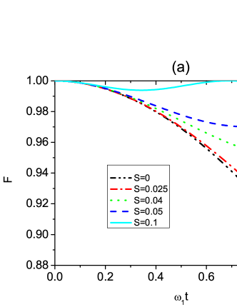
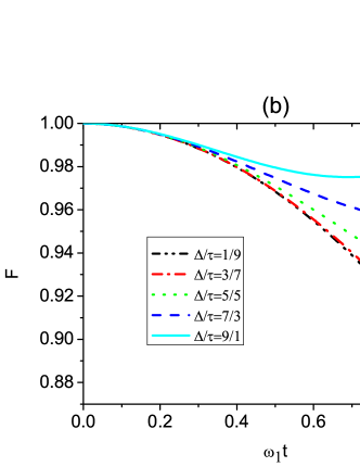
Figure 1: (Color on line) Example 1: Fidelity versus parameter $\omega_{1}t$ for (a) different integral $S$, $\Delta=\xi,\Delta/\tau=1/1,T=1/\omega_{1}$, the time step length we used to calculate is taken as $\xi=0.005/\omega_{1}$; (b) different ratio of $\Delta/\tau$, $\Delta+\tau=10\xi$, $S=0.03$.

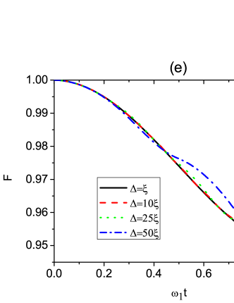
Figure 2: (Color on line) Example 1: Fidelity versus parameter $\omega_{1}t$ for different pulse interval, (a) $\Delta=\xi$; (b) $\Delta=10\xi$; (c)$\Delta=25\xi$; (d) $\Delta=50\xi$. $\Delta/\tau=1/1.$

Now we present the numerical calculation results. Suppose $f(t)$ is chosen as a sequence of rectangular pulses, $f(t)=I$ with control and $f(t)=0$ without control. $I$ is the pulse strength. $\tau(\Delta)$ is the time interval of the free evolution (under control). For a regular rectangular pulse, $\Delta/\tau$ is a constant.

In our numerically calculation we use the time step length $\xi=0.005/\omega_{1}$ to calculate the propagator in Example 1. The integral $S=\int\nolimits_{n\xi}^{(n+1)\xi}f(s^{{}^{\prime}})ds^{{}^{\prime}}$ ($n=0,1,2,...$) in the propagator determines the controllability from Eq. (14). Note that $S$ is a dimensionless parameter.

Suppose the system is initially in the ground state of $H(0)$. The fidelity is defined as $F=\left|\left\langle\Psi(t)|E_{0}(t)\right\rangle\right|$, where $|E_{0}(t)\rangle$ is the instantaneous ground state in Eq. (1) and $|\Psi(t)\rangle$ is the wave function governed by the the time-dependent Schrödinger equation. By numerical calculation, we find that for this example, when $T_{0}\geq 10/\omega_{1}$, the system enters the adiabatic regime ($F>0.995$).

Now in a non-adiabatic regime $T=1/\omega_{{1}}<T_{0}$ we will study the contributions of the pulses. First, we study the effect of pulse strength for regular rectangular pulses. The pulse strengths are taken to be $I=0,5\omega_{1},8\omega_{1},10\omega_{1},20\omega_{1}$, respectively. Fig. 1(a) plots the fidelity as a function of $\omega_{1}t$ for different $S$. It shows that with increasing $S$, the fidelity increases and $F$ approaches one for $S=0.1$ in a non-adiabatic regime. Since the control effect is only determined by the integral of $f(t)$, $F$ will increase with increasing ratio $\Delta/\tau$. Fig. 1(b) shows this property clearly.

Figure 3: (Color on line) Example 1: Different types of pulses, (a) regular rectangular pulses, $\Delta/\tau=5/5$, $\Delta+\tau=10\xi$, $S=0.05$; (b) random rectangular pulses,$\Delta/\tau\in[0,1],\Delta+\tau=20\xi$,$S\in[0,0.1]$; (c) the average values of a thousand times of noises with $S\in(0.047,0.053)$; (d) a fast sine signal $f(t)=10sin^{2}(50t)$.

Does the pulse density affect the control result? In Fig. 2(a)-(d) we plot the fidelity as a function of $\omega_{1}t$ for different pulse intervals with the same ratio. Fig. 2(e) plots the corresponding fidelity. The results show that $F$ changes slightly for same ratio $\Delta/\tau$.

Next we consider different types of pulses. The calculation shows that they work as well as regular rectangular pulses JingPRL2015 ; WangHF . Suppose white noise is present JingPRA2014 , so $f(t)=\eta$rand_ξ(i), here rand(i) is a random number uniformly distributed in the interval $[0,1]$, $\eta=20\omega_{1}$. rand_ξ(i) denotes that random function rand(i) is fixed in the time interval $\xi$, and is random for each time interval. Fig. 3(a)-(d) plot four kinds of pulses: regular rectangular, random rectangular, noise and a fast sine signal $f(t)=10sin^{2}(50t)$. Fig. 3 (b) plots one possible pulse as an example while for Fig. 3(c) we plot an average value of the noises ($S\in(0.047,0.053)$) for different times.

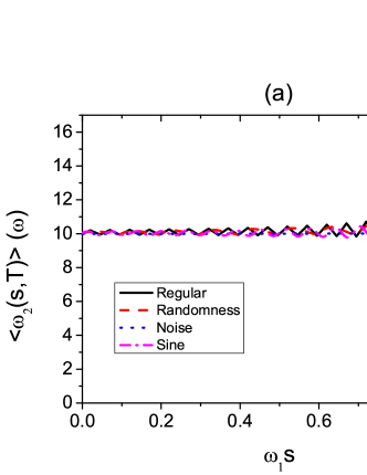
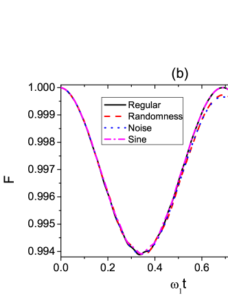
Figure 4: (Color on line) Example 1: For four types of pulses plotted in Fig. 3, (a) average control frequency versus $\omega_{1}s$; (b) the corresponding fidelity versus $\omega_{1}t$. For randomness and noises, we calculate (thousand times) average density matrices and obtain the corresponding average control frequency and fidelity.

In Fig. 4(a) and (b) we plot the corresponding average control frequency and fidelity for four types of pulses plotted in Fig. 3. For randomness and noise, we plot the average control frequency and fidelity for a thousand trials. For the four cases, the average control frequency $\langle\omega_{2}(s,T)\rangle\approx 10\omega_{1}$, except that near $s\rightarrow T$, there exists a fast oscillation. Fig. 4(b) shows that the evolution of the fidelity does not change significantly for near equal average control frequencies. $F(1)\approx 0.994$ for the four cases. Experimentally, producing exactly regular rectangular pulses might not be easy. Our results again relax constraints on experimental implementation of the pulses, whether they are regular, random and even noisy pulse sequences.

Now we turn to Example 2, a 3-spin Heisenberg XY model. The Hamilton is given by

$$H_{0}(t)=\sum\limits_{i=1}^{2}J_{i,i+1}(t)(X_{i}X_{i+1}+Y_{i}Y_{i+1})+\sum\limits_{i=1}^{3}h_{i}(t)Z_{i},$$ (16)

where $J_{i,i+1}(t)$ is the coupling between nearest-neighbor sites. Suppose the coupling changes as $J_{i,i+1}(t)=J\sin(\Omega t)$ and the external field changes as $h_{i}(t)=h_{i}\cos(\Omega t)$, $\Omega=\pi/(2T)$. Due to $[\sum\nolimits_{i}Z_{i},H_{0}(t)]=0$, the magnon is conserved in the evolution. Therefore we only need to discuss the single-excitation subspace where the total number of magnon is one. For simplicity, we take $J=\omega_{1}$ and $h_{1}=\omega_{1},h_{2}=0,h_{3}=-\omega_{1}.$ The Hamiltonian reads

$$H_{0}(t)=\omega_{1}\left(\begin{array}[]{ccc}\cos(\Omega t)&\sin(\Omega t)&0\\ \sin(\Omega t)&0&\sin(\Omega t)\\ 0&\sin(\Omega t)&-\cos(\Omega t)\end{array}\right).$$ (17)

The instantaneous eigenstates $|E_{n}(t)\rangle$ are $|E_{0}(t)\rangle=\cos^{2}(\Omega t/2)|0\rangle-\sin(\Omega t)/\sqrt{2}|1\rangle+\sin^{2}(\Omega t/2)|2\rangle,|E_{1}(t)\rangle=\sin(\Omega t)/2|0\rangle+\sqrt{2}\cos(\Omega t)/2|1\rangle-\sin(\Omega t)/2|2\rangle$, $|E_{2}(t)\rangle=\sin^{2}(\Omega t/2)|0\rangle+\sin(\Omega t)/\sqrt{2}|1\rangle+\cos^{2}(\Omega t/2)|2\rangle$ with eigenvalues $|E_{0}(t)\rangle=-\sqrt{2}\omega_{1},|E_{1}(t)\rangle=0$ and $|E_{2}(t)\rangle=\sqrt{2}\omega_{1}$.

The Hamiltonian in an adiabatic framework with an added LEO control now takes the form

$$H_{0}(t)=\left(\begin{array}[]{ccc}0&-i\Omega/2e^{-i\sqrt{2}\omega_{1}t}&0\\ i\Omega/2e^{i\sqrt{2}\omega_{1}t}&0&-i\Omega/2e^{-i\sqrt{2}\omega_{1}t}\\ 0&i\Omega/2e^{i\sqrt{2}\omega_{1}t}&f(t)\end{array}\right).$$ (18)

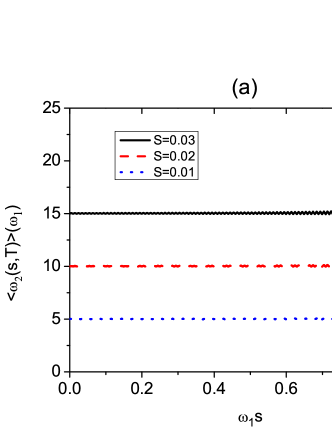
Figure 5: (Color on line) Example 2: (a) The average control frequency $\langle\omega_{2}\rangle$ as function of parameter $\omega_{1}s$; (b) The corresponding fidelity versus parameter $\omega_{1}t$ for different integral $S$, $\Delta=5\xi,\Delta/\tau=1/1,T=1/\omega_{1}$, the time interval we used for the calculations are taken to be $\xi=0.001/\omega_{1}$;

The propagator can be calculated as

$$g^{\prime}(t,s)=-\frac{\Omega^{2}}{4}\cos[\frac{\Omega(t-s)}{2}]\exp\{i[\langle\omega_{2}(s,t)\rangle-\omega_{1}](t-s)\},$$ (19)

where $\langle\omega_{2}(s,t)\rangle$ is the average control frequency defined in Eq. (15). As in the first example, when $\Omega\rightarrow 0$, $g^{\prime}(t,s)\rightarrow 0$, the standard adiabatic conditions are obtained. Compared with Example 1, the propagator $g^{\prime}(t,s)$ is tuned by a cosine function $\cos[\Omega(t-s)/2]$. The adiabaticity can also be enhanced by increasing the average control frequency. For big $\langle\omega_{2}\rangle-\omega_{1}$, the quickly varying factor is $\exp[i(\langle\omega_{2}\rangle-\omega_{1})(t-s)]$ and the slowly varying factor is $\cos[\Omega(t-s)/2]p(s)$. The quickly varying factor eliminates all the off-diagonal elements of the propagator and effective adiabaticity is obtained.

For this example, we consider the non-adiabatic regime where $T=1/\omega_{1}$. Fig. 5 shows (a) a plot of the average control frequency $\langle\omega_{2}(s,T)\rangle$ as a function of parameter $\omega_{1}s$ for different $S$. Fig. 5(b) a plot of the corresponding fidelity. In Fig. 5(b) the dash-dotted curve depicts the fidelity without external pulses. It decays monotonically with time. Clearly when $\langle\omega_{2}\rangle\approx 10$ $\omega_{1}$, $F>0.993$. When $\langle\omega_{2}\rangle\approx 15$ $\omega_{1}$, $F>0.995$, and effective adiabaticity is induced.

IV LEO in experimental framework

The analysis presented above clearly shows that the LEO in an adiabatic frame can be used to prevent transitions. Thus effective adiabaticity is obtained in a non-adiabatic regime. However, the control we add is in the adiabatic frame. What is the experimental manifestation? To see this, we transform to the lab frame. For Example 1,

$$UH_{LEO}U^{{\dagger}} = f(t)[\cos^{2}\omega t/2|0\rangle\langle 0|$$

$$+\sin^{2}\omega t/2 | 1\rangle\langle 1|]$$

$$-(\sin\omega t)/2( | 1\rangle\langle 0|+|0\rangle\langle 1|).$$ (20)

For Example 2,

$$UH_{LEO}U^{{\dagger}}=f(t)|\Phi(t)\rangle\langle\Phi(t)|,$$ (21)

where $|\Phi(t)\rangle=U|E_{0}(t)\rangle=[1-\sin^{2}(\Omega t)/4]|0\rangle-3\sqrt{2}\sin(2\Omega t)/8|1\rangle+3\sin^{2}(\Omega t)/4$ $|2\rangle$. That is to say, if we apply the above pulse control in lab frame, then it is equivalent to adding an LEO in an adiabatic frame.

V Conclusion

Reducing the runtime for quantum information processing tasks is of crucial importance for improving performance. We have introduced an effective control scheme to speed up adiabatic passage by adding an LEO in an adiabatic framework. LEOs WuPRL2002 are general and can be applied to subspaces or subsystems Byrd by using logical operations for the LEO. Here we have shown that for our two examples, the $PQ$ partitioning technique can be used to derive an analytic solution for maintaining the system in an instantaneous eigenstate. Numerical calculations show explicitly that the average control frequency, rather than the details of the control function, determines the control effect JingPRL2015 . This greatly relaxes the constraints of applying regular pulses in experiments. More importantly the control function in an experimental framework is given. This can be applied in the field of adiabatic quantum information processing to improve performance for adiabatic algorithms,

- (1) A. Messiah, Quantum mechanics. North-Holland, Amsterdam. (1962).
- (2) S. Jansen, M.-B. Ruskai, R. and Seiler, J. Math. Phys. 48, 102111 (2007).
- (3) M. S. Sarandy, L.-A. Wu, and D. Lidar, Quantum Inf. Process. 3, 331 (2004).
- (4) V. Srinivasa, J. Levy, and C. S. Hellberg, Phys. Rev. B 76, 094411 (2007).
- (5) V. Balachandran and J. Gong, Phys. Rev. A 77, 012303 (2008).
- (6) U. Farooq, A. Bayat, S. Mancini, and S. Bose, Phys. Rev. B 91, 134303 (2015).
- (7) A. M. Childs, E. Farhi, and J. Preskill, hys. Rev. A 65, 012322 (2001).
- (8) M. S. Sarandy and D. A. Lidar, Phys. Rev. Lett. 95, 250503 (2005).
- (9) P. Zanardi, and M. Rasetti, Phys. Lett. A 264, 94 (1999).
- (10) P. V. Pyshkin, D.-W. Luo, J. Jing, J. Q. You, and L.-A. Wu, Sci. Rep. 6, 37781 (2016) and arXiv:quant-ph/1507.00815 (2015).
- (11) E. Farhi, J. Goldstone, S. Gutmann, J. Lapan, A. Lundgren, and D. Preda, Science, 292, 472 (2001).
- (12) S. Garnerone, P. Zanardi, and D. A. Lidar, Phys. Rev. Lett. 108, 230506 (2012).
- (13) H. Wang and L.-A. Wu, Sci. Rep. 6, 22307 (2016).
- (14) J. Ren, P. H nggi, and B. Li, Phys. Rev. Lett. 104, 170601(2010).
- (15) L.-A. Wu and D. Segal, J. Phys. A: Math. Theor. 42, 025302 (2008).
- (16) K. Bergmann, H. Theuer, and B. W. Shore, Rev. Mod. Phys. 70, 1003 (1998).
- (17) P. Krl, I. Thanopulos, and M. Shapiro, Rev. Mod. Phys. 79, 53 (2007).
- (18) D. Guéry-Odelin, J. G. Muga, Phys. Rev. A 90, 063425 (2014).
- (19) M. V. Berry, J. Phys. A: Math. Theor. 42, 365303 (2009).
- (20) M. Demirplak and S. A. Rice, J. Phys. Chem. A 107, 9937 (2003).
- (21) M. Demirplak and S. A. Rice, J. Phys. Chem. A 129, 154111 (2008).
- (22) J. Jing, L.-A. Wu, T. Yu, J. Q. You, Z.-M. Wang, and L. Garcia, Phys. Rev. A 89, 032110 (2014).
- (23) S. Oh, L.-A. Wu, Y. P. Shim, J. Fei, M. Friesen, X. Hu, Phys. Rev. A 84, 022330 (2011).
- (24) Z.-M. Wang, C.A. Bishop, J. Jing, Y.-J. Gu, C. Garcia, and L.-A. Wu, Phys. Rev. A 93, 062338 (2011).
- (25) L. Voila and S. Lloyd, Phys. Rev. A 58, 2733 (1998).
- (26) L.-A.Wu, M. S. Byrd, and D. A. Lidar, Phys. Rev. Lett.89, 127901 (2002).
- (27) M.S. Byrd, D.A. Lidar, L.-A. Wu, and P. Zanardi, Phys. Rev. A 71, 052301 (2005).
- (28) A. del Campo, I.L. Egusquiza, M.B. Plenio, and S.F. Huelga, Phys. Rev. Lett. 110, 050403 (2013).
- (29) A. del Campo, Phys. Rev. A 84, 031606 (2011).
- (30) J. Jing, L.-A. Wu, M. Byrd, T. Yu, J. Q. You, Z.-M. Wang, Phys. Rev. Lett. 114, 190502 (2015).
- (31) L. Viola, E. Knill, and S. Lloyd, Phys. Rev. Lett. 82, 2417 (1999).
- (32) D. Vitali and P. Tombesi, Phys. Rev. A 59, 4178 (1999).
- (33) L.-A. Wu, G. Kurizki, and P. Brumer, Phys. Rev. Lett. 102, 080405 (2009).