Traveling Solitons in Long-Range Oscillator Chains

We investigate the existence and propagation of solitons in a long-range extension of the quartic Fermi-Pasta-Ulam (FPU) chain of anharmonic oscillators. The coupling in the linear term decays as a power-law with an exponent $1<\alpha\leq 3$. We obtain an analytic perturbative expression of traveling envelope solitons by introducing a Non Linear Schrödinger (NLS) equation for the slowly varying amplitude of short wavelength modes. Due to the non analytic properties of the dispersion relation, it is crucial to develop the theory using discrete difference operators. Those properties are also the ultimate reason why kink-solitons may exist but are unstable, at variance with the short-range FPU model. We successfully compare these approximate analytic results with numerical simulations.

1 Introduction

The study of the equipartition process in the Fermi-Pasta-Ulam-Tsingou (FPU) model of nonlinearly coupled oscillators  [1, 2, 3] has led to important discoveries in both statistical mechanics [4, 5] and nonlinear science [6]. At the same time, nonlinear oscillator chains serve as the simplest prototypes for complex condensed matter systems [7, 8] and biophysical phenomena [9, 10]. In particular, the study of FPU chains has historically motivated the discovery of solitons [11, 12]. Further developments, namely nonintegrable (Klein-Gordon [13] and Frenkel-Kontorova [14]) and integrable Toda [15] chains helped much in understanding the interplay between integrability and chaos [1]. These concepts have been applied to describe transport properties in electric transmission lines [16] and even in quantum systems, such as Josephson junction parallel arrays and lattices [17, 18]. In most cases, the analysis was restricted to one-dimensional ($d=1$) lattices where oscillators interact only with nearest neighbors, i.e. to short-range interactions.

In recent years there has been a growing interest in systems with long-range interactions [19, 20]. In such systems, either the two-body potential or the coupling at separation $r$ decays with a power-law $r^{-\alpha}$. When the power $\alpha$ is less than the dimension of the embedding space $d$, these systems violate additivity, a basic feature of thermodynamics, leading to unusual properties like ensemble inequivalence, broken ergodicity, quasistationary states.

Long-range coupled oscillator models have been previously introduced to cope with dipolar interactions in mechanistic DNA models [21]. They describe also ferroelectric [22] and magnetic [23] systems, where the long-range coupling is provided again by dipolar forces. Other candidates for application are cold gases: dipolar bosons [24, 25], Rydberg atoms [26], atomic ions [27, 28]. Moreover, one can mention optical wave turbulence [29] and scale-free avalanche dynamics [30], where such long-range couplings appear. The extension of the FPU problem to include long-range couplings is rarely considered [31, 32, 33] and attention has been mainly focused on deriving the continuous counterpart of the discrete long range models [32], on considering thermalization properties caused by the long-range character of the interactions [33, 34], or on finding conditions for the existence of standing localized solutions like breathers [31].

In this Letter, we consider a generalization of the FPU model by introducing a long-range coupling in the linear term decaying with the power $\alpha$, while keeping the nonlinear term short-range. We have chosen the power in the range $1<\alpha\leq 3$, where we obtain qualitatively similar results. Below $\alpha=1$ the energy diverges and above $\alpha=3$ the systems becomes short-range. Dipolar systems correspond to the power $\alpha=3$, while the power $\alpha=2$ has been considered for crack front propagation along disordered weak planes between solid blocks [30] and contact lines of liquid spreading on solid surfaces [35].

2 Methods

The Hamiltonian of the model reads

$${\cal H}=\sum\limits_{j=-N}^{N}\frac{p_{j}^{2}}{2}+\frac{1}{2}\sum_{j>\ell=1}^{N}\frac{(u_{j}-u_{\ell})^{2}}{{|j-\ell|}^{\alpha}}+\sum\limits_{\ell=1}^{N}\frac{\left(u_{n+1}-u_{n}\right)^{4}}{4}$$ (1)

and the corresponding equations of motion are

$$\ddot{u}_{\ell}=\sum_{{j=1\\ j\neq\ell}}^{N}\frac{u_{j}-u_{\ell}}{{|j-\ell|}^{\alpha}}+\left(u_{\ell+1}-u_{\ell}\right)^{3}+\left(u_{\ell+1}-u_{\ell}\right)^{3}$$ (2)

Assuming plane wave solutions of the form

$$u_{\ell}=(A/2)e^{i(q\ell-\Omega t)}+c.c.$$ (3)

and substituting them into the equations of motion, we obtain the nonlinear dispersion relation in Rotating Wave Approximation (RWA) for the normal mode frequencies $\Omega_{n}$ and wave numbers $q_{n}$

$$\left(\Omega_{n}\right)^{2}=2\sum_{m=1}^{N}\frac{1-\cos(q_{n}m)}{m^{\alpha}}+3|A|^{2}(1-\cos q_{n})^{2}.$$ (4)

This dispersion relation in the linear limit $A\rightarrow 0$ is shown in the main plot of Fig. 1. The insets show its first derivative $v_{g}$ (group velocity) and second derivative $\Omega^{\prime\prime}$. Derivatives are performed by discrete differences for a sufficiently large finite value of $N$ with step size $h=2\pi/N$. In all calculations below we will the use power-law exponent $\alpha=2$. Both the group velocity $v_{g}$ and $\Omega^{\prime\prime}$ diverge when $N\to\infty$ in the zero wavenumber limit $q_{n}\to 0$.

Let us concentrate first our attention on the solitons that appear at small wavelength. As usual [36], we represent the solution as an expansion in normal modes

$$u_{\ell}=\frac{1}{2}\left[\sum\limits_{n=1}^{N}C_{n}e^{i(q_{n}\ell-\Omega_{n}t)}+c.c.\right].$$ (5)

Focusing on the carrier wavenumber $q^{0}$ of the wave packet and the associated frequency $\Omega^{0}$ in the limit $A\rightarrow 0$, i.e. $\Omega^{0}\equiv\Omega(q^{0},A=0)$, and defining $\Omega_{n}=\Omega^{0}+\epsilon^{2}\delta\Omega_{n}$, $q_{n}=q^{0}+\epsilon\delta q_{n}$, we get an expression of the form of Eq. (3)

$$u_{\ell}=\epsilon\left[A(\zeta,\tau)e^{i(q^{0}\ell-\Omega^{0}t)}+c.c.\right].$$ (6)

where the envelope function $A(\zeta,\tau)$, is a slowly varying function in space $\zeta=\epsilon\ell$ and time $\tau=\epsilon^{2}t$. Its expression is

$$A(\zeta,\tau)=\sum\limits_{n}C_{n}e^{i(\delta q_{n}\zeta-\delta\Omega_{n}\tau)}.$$ (7)

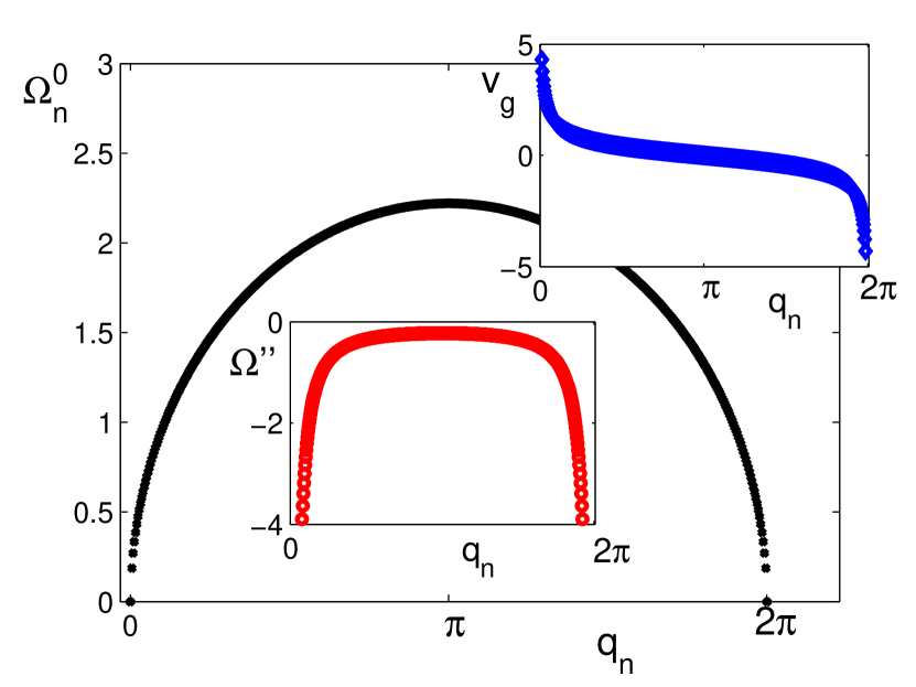
Figure 1: Main plot: dispersion relation (refdisp) in the linear limit $A\rightarrow 0$ for discretized values of the wavenumber $q_{n}=2\pi n/N$, $N=512$. Top inset: the first discrete derivative of the dispersion $v_{g}$ (group velocity). Lower inset: the second discrete derivative $\Omega\prime\prime$.

Taking the time derivative of formula (refA) we get

$$\frac{\partial}{\partial\tau}A(\zeta,\tau)=\sum\limits_{n}C_{n}e^{i(\delta q_{n}\zeta-\delta\Omega_{n}\tau)}\left[-i\delta\Omega_{n}(q_{n})\right].$$ (8)

Expanding now $\epsilon^{2}\delta\Omega_{n}(q_{n})=\Omega_{n}(q_{n})-\Omega^{0}(q^{0})$ around the value $q_{n}^{0}$ and $A=0$ we get approximately

$$\delta\Omega_{n}(q_{n})=\sum_{s=1}^{\infty}\frac{(\epsilon\delta q_{n})^{s}}{\epsilon^{2}s!}\frac{\Delta_{h}^{(s)}\left[{\Omega^{0}(q^{0})}\right]}{h^{s}}+|A|^{2}\frac{\partial\Omega_{n}({q^{0}})}{\partial(|A|^{2})}\biggr{|}_{A=0}$$ (9)

where $\Delta_{h}^{(s)}$ is the difference operator of order $s$ with step size $h=2\pi/N$ in the limit $A=0$. We will restrict ourselves to difference operators of first and second order: $\Delta_{h}^{(1)}{\left[\Omega^{0}\right]\equiv\Omega^{0}(q^{0}+h)-\Omega^{0}(q^{0})}$ and $\Delta_{h}^{(2)}{\left[\Omega^{0}\right]\equiv\Omega^{0}(q^{0}+h)+\Omega^{0}(q^{0}-h)-2\Omega^{0}(q^{0})}$. Then, substituting (reftay) into (refdA) and taking into account the definition (7), we get the following nonlinear equation for the amplitude $A(\zeta,\tau)$

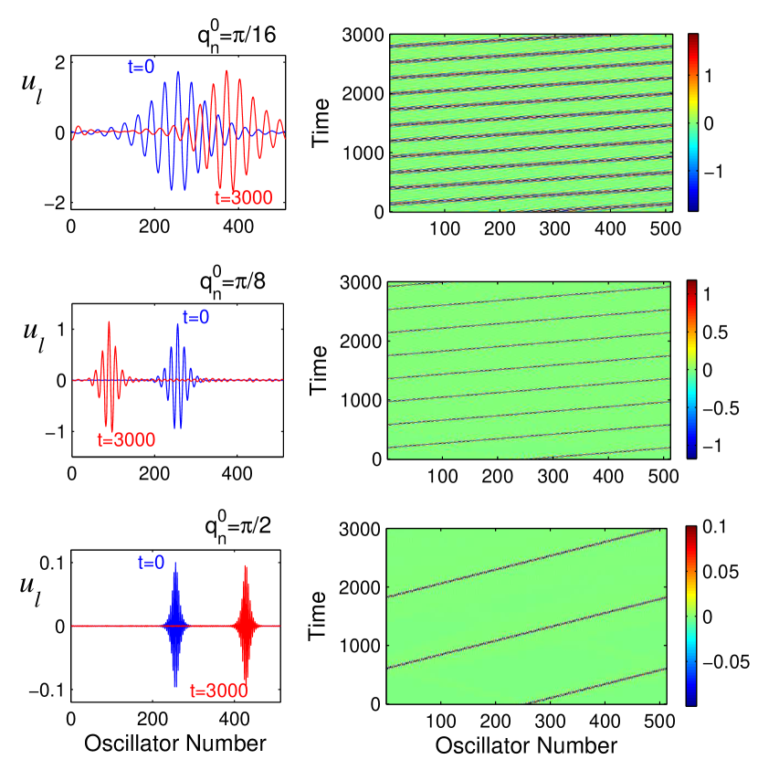
Figure 2: Left panel: Displacement field $u_{l}$ as a function of site number $l$ at times t=0 (blue) and t=3000 (red) for different carrier wavenumbers: $q^{0}=\pi/16,\pi/8$ and $\pi/2$ (from top to bottom). Right panel: Space-time evolution of the displacement field $u_{k}$ represented in color code.

$$i\left(\frac{\partial A}{\partial\tau}+\frac{v_{g}}{\epsilon}\frac{\partial A}{\partial{\zeta}}\right)+\frac{\Omega^{\prime\prime}}{2}\frac{\partial^{2}A}{\partial{\zeta}^{2}}-R|A|^{2}A=0,$$ (10)

where the definitions below have been introduced

$$v_{g}=\Delta_{h}^{(1)}\left[{\Omega^{0}}\right]/h,\qquad\Omega^{\prime\prime}=\Delta_{h}^{(2)}\left[{\Omega^{0}}\right]/h^{2},$$ (11)

$$R=\partial\Omega_{n}({q^{0}})/\partial(|A|^{2})\Bigr{|}_{A=0}={3(1-\cos q^{0})^{2}/2\Omega^{0}}.$$

Now, switching to a comoving reference frame with a rescaled time $t$ and space $\xi$ where $\xi={\epsilon}(\ell-v_{g}t)$, we get the Non Linear Schrödinger (NLS) equation

$$i\frac{\partial A}{\partial t}+\frac{\Omega^{\prime\prime}}{2}\frac{\partial^{2}A}{\partial\xi^{2}}-R|A|^{2}A=0$$ (12)

This equation has the well known one-soliton solution for $A$, which can be inserted in expression (refdef) to get

$$u_{\ell}(t)=\frac{f\cos\left[\left({\Omega^{0}}+\frac{3(1-\cos{q^{0}})^{4}}{4{\Omega^{0}}}f^{2}\right)t-{q^{0}}\ell\right]}{\cosh\left[f(1-\cos{q^{0}})^{2}\sqrt{\frac{3}{2\Omega_{n}^{0}|\Omega^{\prime\prime}|}}(\ell-v_{g}t)\right]},$$ (13)

where $f$ stands for the soliton amplitude.

It is noteworthy to mention that the semi-discrete approach [37, 38, 39] based on the continuous reductive perturbation theory [40] fails in the derivation of the soliton profile (refsoliton2). In particular, a derivation similar to Ref. [37] leads to the same NLS equation (12), but with a different dispersion coefficient containing continuous derivatives $\Omega^{\prime\prime}=\partial^{2}{\Omega^{0}/\partial q^{2}}$ instead of difference operators as given in Eq. (11). The appearance of continuous derivatives causes a divergences of both the group velocity $v_{g}$ and $\Omega^{\prime\prime}$. Indeed, considering continuous derivatives

$$\frac{\partial^{2}{\Omega^{0}}}{\partial q^{2}}=\frac{1}{{\Omega^{0}}}\sum_{m=1}^{N}\frac{\cos(qm)}{m^{\alpha-2}}-\frac{1}{[{\Omega^{0}}]^{3}}\left(\sum_{m=1}^{N}\frac{\sin(qm)}{m^{\alpha-1}}\right),$$ (14)

the first term on the right-hand side is divergent for $\alpha=2$. Specifically, it oscillates as a function of both $q$ and $N$. In summary, the approach in Refs. [37, 38, 39, 40] does not lead to the correct expression for the soliton parameters. The correct approach relies on a discrete wave-packet dynamics [36] and on the use of discrete difference operators, as done in this Letter.

3 Results

We have performed numerical simulations of the set of equations (reffirst) with periodic boundary conditions, using solution (13) as an initial condition ($t=0$), i.e. we consider $u_{\ell}(t=0)$ as initial displacements and $\dot{u}_{\ell}(t=0)$ as initial velocities. In Fig 2 we display the time-evolution of this initial condition for three different wavenumbers, approaching $q^{0}=0$ from bottom to top. As predicted by linear theory the group velocity $v_{g}$ increases when $q^{0}$ decreases. At the same time, the width of the soliton grows as well and thus the wave amplitude must increase in order to keep the soliton within the lattice length limits.

Traveling envelope solitons are robust against perturbations and we do not observe their destruction on a long time scale, while single carrier mode excitation with the same amplitude is modulationally unstable. This instability is presented in Fig.3. The soliton shape (left panel) remains unchanged up to the time $t=10^{4}$, while the single mode excitation (right panel) collapses on a much shorter time interval.

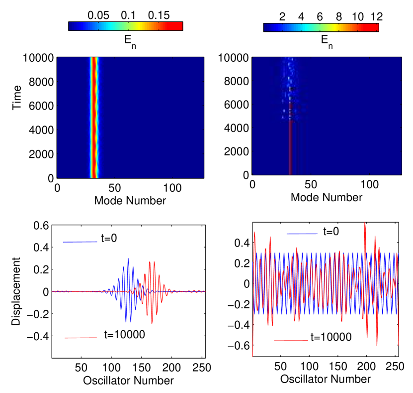
Figure 3: Left panels: Time evolution of solitonic solution (refsoliton2) in mode space (top) and in real space (bottom). Right panel: Time evolution of the single mode in mode space (op) and in real space (bottom). For better visualization only the first 125 modes are displayed, all other modes carry almost zero energy.

One has to mention that the effective nonlinearity parameter in our model is $f\sqrt{R/|\Omega^{\prime\prime}|}$ and we can therefore increase the wave amplitude $f$ in the small carrier wavenumber limit without violating the weak nonlinearity restriction. Beyond this weak nonlinearity limit, traveling envelope solitons become unstable or they are trapped by the lattice and transform into standing breather solutions [31].

The existence of other weakly nonlinear localized solutions, like kink-solitons, is limited by the fast increase of the group velocity in the low wavenumber limit. In fact, low wavenumber excitations, which should in principle generate kink-solitons, are characterized by drastically different velocities and they cannot form localized wave packets obeying the Korteweg-de Vries (KdV) or the modified KdV equations [11, 41, 42, 37]. These problems appear as well in the case of the analytic description of envelope solitons.

However, at strong nonlinearity, kink-soliton solutions with ”magic” wavenumber $2\pi/3$ exist. Extended waves with that particular wavenumber are exact solutions of model (reffirst). It has been proposed that such exact solutions can acquire a compact support and maintain their validity as approximate solutions [43, 44]. These truncated wave solutions can be written in terms of relative displacements as follows

$$u_{\ell+1}-u_{\ell}=\pm\frac{A}{2}\left[1+\cos\left(\frac{2\pi}{3}\ell-\omega t\right)\right]$$ (15)

for $\left|2\pi\ell/3-\omega t\right|<\pi$ and $u_{\ell+1}-u_{\ell}=0$ for $\left|2\pi\ell/3-\omega t\right|>\pi$, where

$$\omega\equiv\Omega(q=2\pi/3,A)=\sqrt{(\Omega_{N/3}^{0})^{2}+(45/16)A^{2}}$$ (16)

and the supersonic kink is characterized by the group velocity $v=3\omega/2\pi$. We have considered here these approximate analytical kink-antikink solutions (refkink) as initial conditions. As far as we use periodic boundary conditions, it is impossible to consider single kink motion: we have thus monitored the dynamics of kink-antikink pairs (see Fig. 4). As it appears from numerical simulations, although the dynamics follows approximately the solution (refkink), the kinks are much less robust against the collisions with perturbative excitations than it happens in the case of envelope solitons. At the beginning the kink shape remains unchanged, but the kink-antikink motion creates perturbations in the lattice and those inhomogeneities finally cause the destruction of the kink solution.

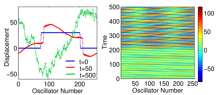
Figure 4: Left panel: Displacement pattern with initial kink-antikink solution (refkink) with amplitude $A=20$ at different time: $t=0$, $t=50$ and $t=500$. Right panel: Color code representation of the evolution of the displacement pattern in space-time of the same kink-antikink pair. As clearly seen, the kink-antikink pair survives up to time $t=200$ after which the system goes to a chaotic regime.

4 Conclusions

Concluding, we have analytically found moving soliton solutions in a long-range version of the FPU model (reffirst). Those are weakly nonlinear envelope solitons and strongly nonlinear kink-soliton solutions. Envelope solitons show stable propagation along the lattice at variance with kink-solitons which collapse on a short time scale. Numerical simulations confirm the validity of the analytic approximate solutions.

5 Acknowledgements

The work is supported in part by contract LORIS (ANR-10-CEXC-010-01). R. Kh. acknowledges financial support from Georgian SRNSF (grant No FR/25/6-100/14) and travel grants from Georgian SRNSF and CNR, Italy (grant No 04/24) and CNRS, France (grant No 04/01).

References

- [1] Chaos, Focus Issue, 15 The ”Fermi-Pasta-Ulam” problem: the first fifty years (2005).
- [2] G. Gallavotti (Editor), The Fermi-Pasta-Ulam problem: a status report, Springer Verlag, Berlin (2008).
- [3] T. Dauxois, Physics Today 61, 55, (2008); T. Dauxois and S. Ruffo, Fermi-Pasta-Ulam nonlinear lattice oscillations, Scholarpedia, 3 (8), 5538 (2008).
- [4] F.M. Izrailev, B.V. Chirikov, Soviet Phys. Dokl. 11, 30 (1966).
- [5] R. Livi, M. Pettini, S. Ruffo, M. Sparpaglione, A. Vulpiani, Phys. Rev. A 28, 3544 (1985).
- [6] A.C. Scott (ed), Encyclopedia of Nonlinear Science, Routledge, New Yourk and London (2005).
- [7] D.K. Campbell, S. Flach, Y.S. Kivshar, Physics Today, 43 (January 2004).
- [8] S. Flach, C.R. Willis, Phys. Rep. 295, 181 (1995).
- [9] S. Takeno, S. Homma, Prog. Theor. Phys. 70, 308 (1983).
- [10] M. Peyrard (ed.), Nonlinear Excitations in Biomolecules, Springer, Berlin (1995).
- [11] N.J. Zabusky, M.D. Kruskal, Phys. Rev. Lett. 15, 240-243 (1965).
- [12] T. Dauxois, M. Peyrard, Physics of Solitons, Cambridge University Press (2005).
- [13] F. Abdullaev, V.V. Konotop, (eds.) Nonlinear Waves: Classical and Quantum Aspects, NATO Science Series II: Mathematics, Physics and Chemistry 153 (2005).
- [14] O.M. Braun, Y.S. Kivshar, The Frenkel-Kontorova Model: Concepts, Methods, and Applications, Springer (2004).
- [15] M. Toda, Jour. Phys. Soc. Japan 22, 431 (1967). M. Toda, Theory of Nonlinear Lattices, Springer (1978).
- [16] D.S. Ricketts, D. Ham, Electrical Solitons: Theory, Design, and Applications, CRC Press (2011).
- [17] P. Binder, D. Abraimov, A.V. Ustinov, S. Flach, Y. Zolotaryuk, Phys. Rev. Lett., 84, 745 (2000).
- [18] D. Chevriaux, R. Khomeriki, J.Leon, Phys. Rev. B, 73, 214516 (2006).
- [19] A. Campa, T. Dauxois T. and S. Ruffo, Phys. Rep., 480, 57 (2009).
- [20] A. Campa, T. Dauxois, D. Fanelli and S. Ruffo, Physics of long-range interacting systems, Oxford University Press (2014).
- [21] Yu. B. Gaididei, S. F. Mingaleev, P. L. Christiansen, R. O. Rasmussen, Phys. Rev. E, 55, 6141 (1997); S. F. Mingaleev, P. L. Christiansen, Yu. B. Gaididei, M. Johansson, K. O. Rasmussen, J. Biol. Phys., 25, 41 (1999); J. Cuevas, F. Palmero, J. F. R. Archilla, F. R. Romero, Phys. Lett. A 299, 221 (2002).
- [22] A. Picinin, M.H. Lente, J.A. Eiras, J.P. Rino, Phys. Rev. B, 69, 064117 (2004).
- [23] Varon M. et al., Sci. Rep., 3 1234 (2013); M.R. Roser, L.R. Corruccini L. R., Phys. Rev. Lett., 65 1064 (1990).
- [24] G. Gori, T. Macry, A. Trombettoni, Phys. Rev. E, 87, 032905 (2013).
- [25] T. Lahaye, C. Menotti, L. Santos, M. Lewenstein and T. Pfau, Rep. Prog. Phys., 72, 126401 (2009).
- [26] R. Heidemann et al., Phys. Rev. Lett., 100, 033601 (2008); P. Schauss et al., Nature (London), 491, 87 (2012).
- [27] R. Bachelard and M. Kastner, Phys. Rev. Lett., 110, 170603 (2013); J. Eisert, M. van den Worm, S. Manmana and M. Kastner, Phys. Rev. Lett., 111, 260401 (2013).
- [28] P. Richerme et al., Nature (London), 511, 198 (2014); P. Jurcevic et al., Nature (London), 511, 202 (2014).
- [29] A. Picozzi, J. Garnier, T. Hansson, P. Suret, S. Randoux, G. Millot, D. N. Christodoulides, Phys. Rep., 541, 1 (2014).
- [30] L. Laurson et al., Nature Communications, 4, 2927, (2013); D. Bonamy, S. Santucci, L. Ponson, Phys. Rev. Lett. 101, 045501 (2008).
- [31] S. Flach, Phys. Rev. E, 58, R4116 (1998); Physica D, 113, 184 (1998).
- [32] V.E. Tarasov, G.M. Zaslavsky, Commun. Nonlinear Sci. Numer. Simul., 11, 885 (2006).
- [33] H. Christodoulidi, C. Tsallis and T. Bountis, Europhys. Lett., 108, 40006 (2014).
- [34] G. Miloshevich, J.P. Nguenang, Th. Dauxois, R. Khomeriki, S. Ruffo, Phys. Rev. E 91, 032927 (2015).
- [35] J.F. Joanny, P.G. De Gennes, J. Chem. Phys. 81, 552 562 (1984).
- [36] J.W. Boyle, S.A. Nikitov, A.D. Boardman, J.G. Booth, K. Booth, Phys. Rev. B, 53, 12173 (1996).
- [37] R. Khomeriki, Phys. Rev. E, 65, 026605, (2002).
- [38] N. Giorgadze and R. Khomeriki, Phys. Rev. B 60, 1247 (1999).
- [39] L. Chotorlishvili, R. Khomeriki, A. Sukhov, S. Ruffo, J. Berakdar, Phys. Rev. Lett. 111, 117202 (2013).
- [40] T. Taniuti, N. Yajima, J. Math. Phys., 10, 1369, (1969).
- [41] Yu. A. Kosevich, Phys. Rev. B, 47 3138 (1993); 48, 3580 (1993).
- [42] P. Poggi, S. Ruffo, H. Kantz, Phys. Rev. E, 52, 307 (1995).
- [43] Yu. A. Kosevich, Phys. Rev. Lett., 71 2058 (1993).
- [44] Yu. A. Kosevich, R. Khomeriki, S. Ruffo, Europhysics Letters, 66, 21 (2004).