Ferromagnetic order induced on graphene by Ni/Co proximity effects

Abstract

We build a tight-binding Hamiltonian describing Co/Ni over graphene, contemplating ATOP (a Co/Ni atom on top of each Carbon atom of one graphene sublattice) and HCP (one Co/Ni atom per Graphene plaquette) configurations. For the ATOP configuration the orbitals involved, for the Co/Ni, are the $d_{z^{2}-r^{2}}$ which most strongly couples to one graphene sublattice and the $d_{xz}$, $d_{yz}$ orbitals that couple directly to the second sublattice site. Such configuration is diagonal in pseudo-spin and spin space, yielding electron doping of the graphene and antiferro-magnetic ordering in the primitive cell in agreement with DFT calculations. The second, HCP configuration is symmetric in the graphene sublattices and only involves coupling to the $d_{xz}$, $d_{yz}$ orbitals. The register of the lattices in this case allows for a new coupling between nearest neighbour sites, generating non-diagonal terms in the pseudo-spin space and novel spin-kinetic couplings mimicking a spin-orbit coupling generated by a magnetic coupling. The resulting proximity effect in this case yields ferromagnetic order in the graphene substrate. We derive the band structure in the vicinity of the K points for both configurations, the Bloch wavefunctions and their spin polarization.

I Introduction

Graphene-like two dimensional structures have captured the imagination of experimentalists for practical applications, because of the high hole/electron densities ($10^{13}{\rm cm}^{-2}$ much larger than GaAs electron gas) achieved by gatingNovoselov at a small fraction of the cost and complexity of producing a two dimensional electron gas with well known semi-conductor technologies. One can also build semi-conductors from graphene by breaking the sublattice A/B symmetry, in systems such as Boron-NitrideSongBoronNitride , generating a gap ($\sim 5$ eV) at the K point with a quadratic dispersion. Because it is undesiderable to introduce substitutional impurities to modify graphene’s properties, due to the rapid degradation of electron mobilities, one can resort to proximity effectsJapCoGraphene in order for graphene to inherit potentially useful couplings and properties such as a strong Spin-orbit couplingMarchenko2012 , magnetismWangProximity and even chiralityOstovar . Deposited transition metals such as Co and Ni have matching lattice constants and a few layers easily form on graphene with a large perpendicular magnetic anisotropyMagneticAnisot . Such magnetic layers can be used to introduce new effective couplings between graphene $p_{z}$ orbitals, thus inducing a strong Rashba type coupling, inherited from the Co/Ni overlayer, and also an electron spin polarization with perturbative modifications of the electron mobility.

In this article we consider tight-binding modelling of Co/Ni on planar graphene in two configurations. As found by DFT calculationsMacdonald2013 , the lowest energy configuration corresponds to one sub-lattice site of the graphene atop a Co/Ni atom while the neighbouring sub-lattice atom is in a Co/Ni hcp site. For this configuration, ref.Macdonald2013, has shown that the graphene inherits an antiferromagnetic order due mostly to the sublattice asymmetry of the coupling between $p_{z}$ orbitals of Carbon and the Co. This type of order lends itself to enhanced RKKY interactions between Co islands on grapheneVozMediano , that can be tuned to be either ferro or anti-ferro by gate control.

The second configuration we consider corresponds to a global lattice shift from the previous one where all graphene carbon sites fall at HCP sites of the Co/Ni layer. Referring to the detailed DFT study of ref.Macdonald2013, we will first derive the tight-binding model for the first configuration by describing the orbital overlaps and chemical potentials. We then use such parameterization to estimate the corresponding ones from the second configuration. While the first configuration yields anti-ferro order on graphene, the second configuration is symmetric between A/B sublattices and yields ferromagnetic order in the graphene plane.

The summary of this paper is as follows: In section II we describe the two different registers we consider for the tight binding model. Focusing first on the ATOP configuration we identify the most salient overlaps involved between the carbon $p_{z}$ orbitals and the $d$ orbitals of Co/Ni (considering only nearest neighbour overlaps), and derive using the band folding scheme, the effective Hamiltonian for $\pi-$electrons of graphene in the presence of the magnetic overlayer. Next, we shift the lattice register and consider the HCP configuration, where now the configuration is such that non-diagonal pseudo-spin terms arise, coupling A and B sublattices. In section III we obtain the Bloch Hamiltonians for both configurations and determine the band structure and wavefunctions for the bulk samples. The new HCP configuration displays a non-trivial ferromagnetic ordering and a spin dependent kinetic term proportional to the spin-splitting energy of the Co/Ni covering. Finally, we discuss spin related properties of the new Hamiltonians for biased and equilibrium current setups.

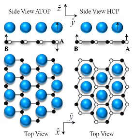
Figure 1: Schematic picture of the configurations of a Co monolayer adsorbed on graphene. (Left) ATOP configuration: Co atoms are directly over the atoms of sublattice A and atoms of the sublattice B are in the hcp sites. (Right) HCP configuration: atoms of the sublattices A and B are at hcp sites. In both cases the magnetic order of cobalt, as well as the resulting magnetic order of the sublattices A and B, is indicated.

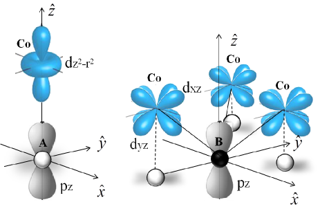
Figure 2: Positions of the Co first neighbor around A (left) and B (right), for the ATOP configuration. The orbitals that intervene in the overlaps of Co with A and B are drawn in each case.

II ATOP and HCP configurations and band folding

Our system consists of a monolayer of Co atoms adsorbed on graphene. A bilayer of Co was shown to be stableMacdonald2013 sustaining a strong anisotropy with magnetization per atom close to the bulk values. For the model derived here, we only take into account graphene interactions with the first adsorbed layer. We consider two registries for the positions of the Co atoms with respect to graphene atoms belonging to the sublattices A and B, which are shown in Fig. 1. In the configuration of Fig. 1(left) (ATOP configuration) the C atoms of the sublattice A are directly under the Co atoms, while atoms of sublattice B are at the hcp sites of the cobalt lattice. In the configuration of Fig. 1(right) (HCP configuration), both sublattice atoms are at hcp sites of Co. In the model computations, the first neighbour approximation is used. We will consider that Co is magnetized in the positive $\hat{z}$ direction (see Fig. 1). The intrinsic spin-orbit interaction (SOI) and the Rashba coupling will not be addressed here since further overlaps will be involved beyond the $d$ orbitals of the Co. Nevertheless, in the absence of magnetism, the SOI is the only coupling generating spin effects and should be taken into account for interface metals such as PbBrey and AuMarchenko2012 to assess e.g. the enhancement of topological properties of graphene. The SOI due to changes in the hybridization of carbon in graphene as a result of deformations of the surface due to corrugation or hydrogenationCastroNeto will be left to future work.

II.1 ATOP configuration

In the ATOP configuration, as shown in the left of Fig. 2, the orbital $p_{z}$ of a C atom A, $Ap_{z}$, has greatest overlap with the orbital $d_{z^{2}-r^{2}}$ (in short $d_{z^{2}}$), of the Co layer. For the neighbouring B atom (see the right of Fig. 2), the orbital $p_{z}$, $Bp_{z}$, overlaps preferentially with the orbitals $d_{xz}$ and $d_{yz}$ of the first neighbour Co atoms (there are three Co atoms around each B atom of graphene). The graphene-Co coupled Hamiltonian for the ATOP configuration is the following

$$H_{\rm ATOP}=\begin{bmatrix}\begin{matrix}Ap_{z}&Bp_{z}\end{matrix}&\begin{matrix}d_{z^{2}-r^{2}}&&&&d_{xz}&&&&d_{yz}\end{matrix}\\ \begin{bmatrix}\varepsilon_{p}&V_{pp\pi}\\ V^{*}_{pp\pi}&\varepsilon_{p}\\ \\ \end{bmatrix}&\begin{bmatrix}V_{pdz}&&&&0&&&&0\\ 0&&&&\hat{n}_{x}\widetilde{V}_{pd\pi}&&&&\hat{n}_{y}\widetilde{V}_{pd\pi}\\ \\ \end{bmatrix}\\ \begin{bmatrix}-V_{pdz}&0\\ 0&-\hat{n}_{x}\widetilde{V}_{pd\pi}\\ 0&-\hat{n}_{y}\widetilde{V}_{pd\pi}\end{bmatrix}&\begin{bmatrix}\varepsilon_{dz^{2}}+\delta_{1}S_{z}&0&0\\ 0&\varepsilon_{dxz}+\delta_{2}S_{z}&0\\ 0&0&\varepsilon_{dyz}+\delta_{2}S_{z}\\ \end{bmatrix}\end{bmatrix}.$$ (1)

where the array consists of four sub-spaces. The upper left sub-space contains the bare $p_{z}$-orbital site energies of graphene $\varepsilon_{p}$, and the off-diagonal overlaps $V_{pp\pi}$, between A-B sites. The upper right subspace contains the overlaps between the orbitals $Ap_{z}$ and $Bp_{z}$ with the orbitals $d_{z^{2}}$, $d_{xz}$ and $d_{yz}$ which are $V_{pdz}$, ${\hat{n}_{x}}\widetilde{V}_{pd\pi}$ and ${\hat{n}_{y}}\widetilde{V}_{pd\pi}$ (computed below), respectively, where ${\hat{n}_{x},\hat{n}_{y}}$ are the corresponding direction cosines in a Slater-Koster constructionSlaterKoster ; Konschuh . Note that the lower left submatrix is the negative of the upper right submatrix since $\langle l^{\prime}|H|l\rangle=(-1)^{l+l^{\prime}}\langle l|H|l^{\prime}\rangle$ (see ref.Konschuh, ) where $l$ is the orbital angular momentum quantum number ($l=1$ for $p$ and $l=2$ for $d$ orbitals).

Finally, the lower right sub-space contains, in the diagonal, the energies of the coupled $d$ orbitals, $\varepsilon_{z^{2}}$, $\varepsilon_{xz}$ and $\varepsilon_{yz}$. As we are considering that Co is magnetized in the $\hat{z}$ direction, we add to the $d$ orbital energies the Stoner exchange splittings $\delta_{1}$ for the orbital $d_{z^{2}}$ and $\delta_{2}$ for the orbitals $d_{xz}$ and $d_{yz}$. We assume that $d_{xz}$ and $d_{yz}$ have the same exchange coupling. $S_{z}$ is the $z$ component Pauli matrix.

The overlaps between orbitals $p_{z}$ and, $d_{xz}$ and $d_{yz}$, are calculated using the relations SlaterKoster ; Konschuh

$$\begin{split}\langle Bp_{z}|H_{1}|d_{xz}\rangle&=\sqrt{3}n_{z}^{2}n_{x}V_{pd\sigma}+n_{x}(1-2n_{z}^{2})V_{pd\pi},\\ \langle Bp_{z}|H_{1}|d_{yz}\rangle&=\sqrt{3}n_{z}^{2}n_{y}V_{pd\sigma}+n_{y}(1-2n_{z}^{2})V_{pd\pi},\end{split}$$ (2)

where $n_{x}$, $n_{y}$ and $n_{z}$ are the direction cosines. Both overlaps have a common factor that only depends on $n_{z}$, $V_{pd\sigma}$ and $V_{pd\pi}$. In spherical coordinates $n_{z}=\cos\phi$, where $\phi$ is the polar angle. The first three neighbours, B, of the ATOP site share the same $\phi$ angle. Replacing $n_{x}=\cos\theta\sin\phi$ and $n_{y}=\sin\theta\sin\phi$, where $\theta$ is the azimuthal angle in the graphene plane and defining

$$\widetilde{V}_{pd\pi}=\sin\phi(\sqrt{3}n_{z}^{2}V_{pd\sigma}+(1-2n_{z}^{2})V_{pd\pi}),$$ (3)

which is a common term for both overlaps, we have

$$\begin{split}\langle Bp_{z}|H_{1}|d_{xz}\rangle&=\hat{n}_{x}\widetilde{V}_{pd\pi},\\ \langle Bp_{z}|H_{1}|d_{yz}\rangle&=\hat{n}_{y}\widetilde{V}_{pd\pi},\end{split}$$ (4)

where $\hat{n}_{x}=\cos\theta$ and $\hat{n}_{y}=\sin\theta$.

The eigenvalue equation for Eq.1 has the form

$$\left(\begin{array}[]{cccc}H_{\gamma}&T\\ T^{\dagger}&H_{\chi}\\ \end{array}\right)\left(\begin{array}[]{cc}\gamma\\ \chi\end{array}\right)=E\left(\begin{array}[]{cc}\gamma\\ \chi\end{array}\right),$$ (5)

with

$$H_{\gamma} = \left(\begin{array}[]{cccc}0&V_{pp\pi}\\ V^{*}_{pp\pi}&0\\ \end{array}\right)~{};~{}T=\left(\begin{array}[]{cccc}V_{pdz}&0&0\\ 0&\hat{n}_{x}\widetilde{V}_{pd\pi}&\hat{n}_{y}\widetilde{V}_{pd\pi}\\ \end{array}\right),$$ (10)

$$H_{\chi} = \left(\begin{array}[]{cccccc}(\varepsilon_{dz^{2}}+\delta_{1}S_{z})-\varepsilon_{p}&0&0\\ 0&(\varepsilon_{dxz}+\delta_{2}S_{z})-\varepsilon_{p}&0\\ 0&0&(\varepsilon_{dyz}+\delta_{2}S_{z})-\varepsilon_{p}\\ \end{array}\right),$$ (14)

where we have taken the energy of the orbital $p_{z}$ of graphene as the reference of zero energy, subtracting $\varepsilon_{p}$ to the diagonals of $H_{\gamma}$ and $H_{\chi}$. The wave function subspaces $\gamma=\left(\psi_{Ap_{z}},\psi_{Bp_{z}}\right)$ and $\chi=\left(\psi_{z^{2}-r^{2}},\psi_{xz},\psi_{yz}\right)$ are coupled by $T$. Eliminating the wavefunction subspace of the Co overlayer ($\chi$) one arrives at

$$\left[H_{\gamma}+T\left(E-H_{\chi}\right)^{-1}T^{\dagger}\right]\gamma=E\gamma,$$ (15)

where we have “folded” all the information about the couplings and the Co Hamiltonian into a graphene effective coupling between A and B sublattices and renormalized the site energies. To linear order in $E$ and lowest order in the coupling $T$, we can expand the inverse operator so that we obtain

$$\left[H_{\gamma}-TH^{-1}_{\chi}T^{\dagger}\right]\gamma\approx ES\gamma,$$ (16)

where $S=1+TH^{-2}_{\chi}T^{\dagger}$. Now one defines $\Phi=S^{1/2}\gamma$, a function which is normalized $|\Phi|^{2}\approx\gamma^{\dagger}\gamma+\chi^{\dagger}\chi$ to the same order as the new effective Hamiltonian. The final expression is then

$$S^{-1/2}\left[H_{\gamma}-TH^{-1}_{\chi}T^{\dagger}\right]S^{-1/2}\Phi\approx E\Phi.$$ (17)

The effective Hamiltonian for graphene accounting for its interactions with Co is

$$H_{\rm eff}=S^{-1/2}\left[H_{\gamma}-TH^{-1}_{\chi}T^{\dagger}\right]S^{-1/2}.$$ (18)

The inverse of the matrix $H_{\chi}$ is then

$$H_{\chi}^{-1}=\left(\begin{array}[]{cccc}-\frac{(\varepsilon_{p}-\varepsilon_{d})+\delta_{1}S_{z}}{(\varepsilon_{p}-\varepsilon_{d})^{2}-\delta_{1}^{2}}&0&0\\ 0&-\frac{(\varepsilon_{p}-\varepsilon_{d})+\delta_{2}S_{z}}{(\varepsilon_{p}-\varepsilon_{d})^{2}-\delta_{2}^{2}}&0\\ 0&0&-\frac{(\varepsilon_{p}-\varepsilon_{d})+\delta_{2}S_{z}}{(\varepsilon_{p}-\varepsilon_{d})^{2}-\delta_{2}^{2}}\end{array}\right),$$ (19)

so the product $TH_{\chi}^{-1}T^{{\dagger}}$ is expanded as

$$TH_{\chi}^{-1}T^{{\dagger}}=\left(\begin{array}[]{cccc}V_{pdz}&0&0\\ 0&\hat{n}_{mx}\widetilde{V}_{pd\pi}&\hat{n}_{my}\widetilde{V}_{pd\pi}\end{array}\right)\left(\begin{array}[]{cccc}-\frac{(\varepsilon_{p}-\varepsilon_{d})+\delta_{1}S_{z}}{(\varepsilon_{p}-\varepsilon_{d})^{2}-\delta_{1}^{2}}&0&0\\ 0&-\frac{(\varepsilon_{p}-\varepsilon_{d})+\delta_{2}S_{z}}{(\varepsilon_{p}-\varepsilon_{d})^{2}-\delta_{2}^{2}}&0\\ 0&0&-\frac{(\varepsilon_{p}-\varepsilon_{d})+\delta_{2}S_{z}}{(\varepsilon_{p}-\varepsilon_{d})^{2}-\delta_{2}^{2}}\end{array}\right)\left(\begin{array}[]{cccc}-V_{pdz}&0\\ 0&-\hat{n}_{mx}\widetilde{V}_{pd\pi}\\ 0&-\hat{n}_{my}\widetilde{V}_{pd\pi}\end{array}\right),$$

where we have included the subindex $m$ to the cosine directors $\hat{n}_{mx,my}$ to indicate that for each of the three Co atoms surrounding a B type atom on graphene (see Fig. 2), we have a different overlap. The product becomes the simple diagonal expression

$$TH_{\chi}^{-1}T^{{\dagger}}=$$ (22)

$$\left(\begin{array}[]{cccc}\frac{(\varepsilon_{p}-\varepsilon_{d})+\delta_{1}S_{z}}{(\varepsilon_{p}-\varepsilon_{d})^{2}-\delta_{1}^{2}}V_{pdz}^{2}&0\\ 0&\frac{(\varepsilon_{p}-\varepsilon_{d})+\delta_{2}S_{z}}{(\varepsilon_{p}-\varepsilon_{d})^{2}-\delta_{2}^{2}}\widetilde{V}_{pd\pi}^{2}[\hat{n}_{mx}^{2}+\hat{n}_{my}^{2}]\end{array}\right).$$

The Hamiltonian for the ATOP configuration is obtained substituting Eq. (22) into Eq. (18), approximating $S\sim\mathbbm{1}$ and performing the sum $\sum_{m=1}^{3}[{n}_{mx}^{2}+{n}_{my}^{2}]=3$, which accounts for the contribution to the site energy due to hops of electrons that go from B to Co and return back to B (see ref.PastawskiMedina, ). The effective Hamiltonian is then

$$H_{\rm ATOP}\approx H_{\gamma}-\left(\begin{array}[]{cccc}\frac{(\varepsilon_{p}-\varepsilon_{d})+\delta_{1}S_{z}}{(\varepsilon_{p}-\varepsilon_{d})^{2}-\delta_{1}^{2}}V_{pdz}^{2}&0\\ 0&3\frac{(\varepsilon_{p}-\varepsilon_{d})+\delta_{2}S_{z}}{(\varepsilon_{p}-\varepsilon_{d})^{2}-\delta_{2}^{2}}\widetilde{V}_{pd\pi}^{2}\end{array}\right).$$ (24)

In second quantized form, the Hamiltonian for the full Brillouin zone can be written as

$$H_{\rm ATOP}={-\sum_{\langle ij\rangle}\gamma_{0}a_{i}^{{\dagger}}b_{j}}-\frac{(\varepsilon_{p}-\varepsilon_{d})+\delta_{1}S_{z}}{(\varepsilon_{p}-\varepsilon_{d})^{2}-\delta_{1}^{2}}V_{pdz}^{2}\sum_{i}a_{i}^{{\dagger}}a_{i}-3\frac{(\varepsilon_{p}-\varepsilon_{d})+\delta_{2}S_{z}}{(\varepsilon_{p}-\varepsilon_{d})^{2}-\delta_{2}^{2}}\widetilde{V}_{pd\pi}^{2}\sum_{j}b_{j}^{{\dagger}}b_{j},$$ (25)

where $\gamma_{0}=-V_{pp\pi}$ is the regular off-diagonal kinetic term in graphene and $a_{i}$ and $b_{j}$ are the annihilation operators in the sites A and B graphene sublattices.

II.2 HCP configuration

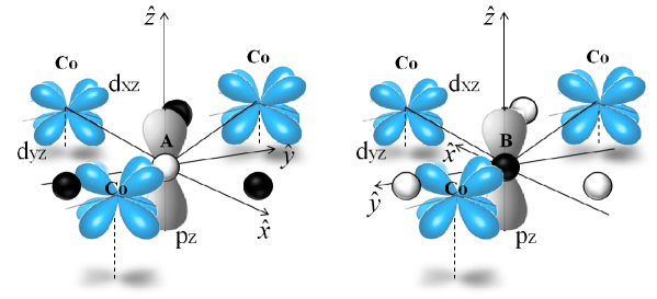
Figure 3: Positions of the Co first neighbor around A (left) and B (right), for the HCP configuration. The orbitals that intervene in the overlaps of Co with A and B are drawn in each case.

For the lattice symmetric or HCP configuration, the orbital $d_{z^{2}}$ does not intervene as in the previous case due to the relative positions of the Co and graphene atoms, as all graphene sites now see the Co/Ni as the B sites in the ATOP configuration. The overlap matrix is given by

$$\begin{bmatrix}\begin{matrix}Ap_{z}&Bp_{z}\end{matrix}&\begin{matrix}d_{z^{2}-r^{2}}&&&d_{xz}&&&d_{yz}\end{matrix}\\ \begin{bmatrix}\varepsilon_{p}&V_{pp\pi}\\ V^{*}_{pp\pi}&\varepsilon_{p}\\ \\ \end{bmatrix}&\begin{bmatrix}0&&&&\hat{n}_{x}\widetilde{V}_{pd\pi}&&&&\hat{n}_{y}\widetilde{V}_{pd\pi}\\ 0&&&&\hat{n}_{x}\widetilde{V}_{pd\pi}&&&&\hat{n}_{y}\widetilde{V}_{pd\pi}\\ \\ \end{bmatrix}\\ \begin{bmatrix}0&0\\ -\hat{n}_{x}\widetilde{V}_{pd\pi}&-\hat{n}_{x}\widetilde{V}_{pd\pi}\\ -\hat{n}_{y}\widetilde{V}_{pd\pi}&-\hat{n}_{y}\widetilde{V}_{pd\pi}\end{bmatrix}&\begin{bmatrix}\varepsilon_{dz^{2}}+\delta_{1}S_{z}&0&0\\ 0&\varepsilon_{dxz}+\delta_{2}S_{z}&0\\ 0&0&\varepsilon_{dyz}+\delta_{2}S_{z}\\ \end{bmatrix}\end{bmatrix}.$$ (26)

In this case A and B see the same environment of three Co atoms at the same distance, as can be seen in Fig. 3. Both graphene sites interact with them through the orbitals $d_{xz}$ and $d_{yz}$.

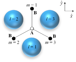
Figure 4: Positions of the Co and B carbon atoms around a carbon atom A, in the HCP configuration of Co/graphene. $l=1,2,3$ represents the Co surrounding A, and $m=1,2,3$ represents the hops from A to B.

The product $TH_{\chi}^{-1}T^{{\dagger}}$ is now

$$TH_{\chi}^{-1}T^{{\dagger}}=\left(\begin{array}[]{cccc}0&\hat{n}_{lx}\widetilde{V}_{pd\pi}&\hat{n}_{ly}\widetilde{V}_{pd\pi}\\ 0&\hat{n}_{lmx}\widetilde{V}_{pd\pi}&\hat{n}_{lmy}\widetilde{V}_{pd\pi}\end{array}\right)\left(\begin{array}[]{cccc}-\frac{(\varepsilon_{p}-\varepsilon_{d})+\delta_{1}S_{z}}{(\varepsilon_{p}-\varepsilon_{d})^{2}-\delta_{1}^{2}}&0&0\\ 0&-\frac{(\varepsilon_{p}-\varepsilon_{d})+\delta_{2}S_{z}}{(\varepsilon_{p}-\varepsilon_{d})^{2}-\delta_{2}^{2}}&0\\ 0&0&-\frac{(\varepsilon_{p}-\varepsilon_{d})+\delta_{2}S_{z}}{(\varepsilon_{p}-\varepsilon_{d})^{2}-\delta_{2}^{2}}\end{array}\right)\left(\begin{array}[]{cccc}0&0\\ -\hat{n}_{lx}\widetilde{V}_{pd\pi}&-{\hat{n}_{lmx}}\widetilde{V}_{pd\pi}\\ -{\hat{n}_{ly}}\widetilde{V}_{pd\pi}&-\hat{n}_{lmy}\widetilde{V}_{pd\pi}\end{array}\right),$$

where, as before, $\hat{n}_{l}$ denote direction cosines in the plane that go from the site A to the Co $l=1,2,3$ (A-Co direction) and $\hat{n}_{lm}$ are direction cosines in the plane that go from the site B to the Co $l=1,2,3$ (B-Co direction). Performing the product we have:

$$TH_{\chi}^{-1}T^{{\dagger}}=\left(\begin{array}[]{cccc}\frac{(\varepsilon_{p}-\varepsilon_{d})+\delta_{2}S_{z}}{(\varepsilon_{p}-\varepsilon_{d})^{2}-\delta_{2}^{2}}\widetilde{V}_{pd\pi}^{2}[\hat{n}_{lx}^{2}+\hat{n}_{ly}^{2}]&\frac{(\varepsilon_{p}-\varepsilon_{d})+\delta_{2}S_{z}}{(\varepsilon_{p}-\varepsilon_{d})^{2}-\delta_{2}^{2}}\widetilde{V}_{pd\pi}^{2}[\hat{n}_{lx}\hat{n}_{lmx}+{\hat{n}_{ly}}\hat{n}_{lmy}]\\ \frac{(\varepsilon_{p}-\varepsilon_{d})+\delta_{2}S_{z}}{(\varepsilon_{p}-\varepsilon_{d})^{2}-\delta_{2}^{2}}\widetilde{V}_{pd\pi}^{2}[\hat{n}_{lx}\hat{n}_{lmx}+{\hat{n}_{ly}}\hat{n}_{lmy}]&\frac{(\varepsilon_{p}-\varepsilon_{d})+\delta_{2}S_{z}}{(\varepsilon_{p}-\varepsilon_{d})^{2}-\delta_{2}^{2}}\widetilde{V}_{pd\pi}^{2}[\hat{n}_{lmx}^{2}+\hat{n}_{lmy}^{2}]\end{array}\right).$$ (27)

The Hamiltonian for the symmetric configuration is obtained substituting Eq. (27) into Eq. (18), and that $\sum_{l=1}^{3}[{n}_{lx}^{2}+{n}_{ly}^{2}]=3$, which accounts for the contribution to the site energy of hops of electrons that go from A to Co and return back to A. $\sum_{m,l=1}^{3}[{n}_{lmx}^{2}+{n}_{lmy}^{2}]=3$ given that ${n}_{lmx}=\cos\theta^{\prime}$ and ${n}_{lmy}=\sin\theta^{\prime}$ where $\theta^{\prime}$ is the azimuthal angle for the overlap between site B and the Co orbitals. The latter sum accounts for the contribution to the site energy of hops of electrons that go from B to Co and return back to B.

Finally we have the somewhat more complicated summation $\sum_{m,l=1}^{3}[\hat{n}_{lx}\hat{n}_{lmx}+{\hat{n}_{ly}}\hat{n}_{lmy}]$ which is performed in detail in the appendix. The Hamiltonian for this configuration is then

$$H_{\rm HCP}\approx H_{\gamma}-\left(\begin{array}[]{cccc}3\frac{(\varepsilon_{p}-\varepsilon_{d})+\delta_{2}S_{z}}{(\varepsilon_{p}-\varepsilon_{d})^{2}-\delta_{2}^{2}}\widetilde{V}_{pd\pi}^{2}&-\frac{(\varepsilon_{p}-\varepsilon_{d})+\delta_{2}S_{z}}{(\varepsilon_{p}-\varepsilon_{d})^{2}-\delta_{2}^{2}}\widetilde{V}_{pd\pi}^{2}\\ -\frac{(\varepsilon_{p}-\varepsilon_{d})+\delta_{2}S_{z}}{(\varepsilon_{p}-\varepsilon_{d})^{2}-\delta_{2}^{2}}\widetilde{V}_{pd\pi}^{2}&3\frac{(\varepsilon_{p}-\varepsilon_{d})+\delta_{2}S_{z}}{(\varepsilon_{p}-\varepsilon_{d})^{2}-\delta_{2}^{2}}\widetilde{V}_{pd\pi}^{2}\end{array}\right),$$ (28)

The complete HCP Hamiltonian, in terms of the creation and annihilation operators in the sites A and B of graphene, $a_{i}$ and $b_{j}$, is given by

$$H_{\rm HCP}=\Big{(}{-\gamma_{0}}+\frac{(\varepsilon_{p}-\varepsilon_{d})+\delta_{2}S_{z}}{(\varepsilon_{p}-\varepsilon_{d})^{2}-\delta_{2}^{2}}\widetilde{V}_{pd\pi}^{2}\Big{)}\sum_{\langle ij\rangle}a_{i}^{{\dagger}}b_{j}-3\frac{(\varepsilon_{p}-\varepsilon_{d})+\delta_{2}S_{z}}{(\varepsilon_{p}-\varepsilon_{d})^{2}-\delta_{2}^{2}}\widetilde{V}_{pd\pi}^{2}\Big{(}\sum_{i}a_{i}^{{\dagger}}a_{i}+\sum_{j}b_{j}^{{\dagger}}b_{j}\Big{)},$$ (29)

III Band structure and magnetic order of the Cobalt/graphene system

We now derive the Hamiltonians in reciprocal space in order to determine the band structures of graphene modified by adsorbed and polarized Co/Ni in both ATOP and HCP configurations. The Bloch Hamiltonian is derived by computing the following matrix elements in pseudo-spin space

$$H_{\rm AA}(\mathbf{k}) = \frac{1}{N}\sum_{l=1}^{N}\sum_{j=1}^{N}e^{i\mathbf{k}\cdot(\mathbf{R}_{Aj}-\mathbf{R}_{Al})}\langle\phi_{Al}|H|\phi_{Aj}\rangle$$ (30)

$$= H_{\rm BB}(\mathbf{k})$$

where $N$ is the number of unit cells, $\mathbf{k}$ is the Bloch wavevector and we take $(\mathbf{R}_{Aj}-\mathbf{R}_{Al})=0$ since we do not consider second neighbour interactions (only $j=l$ terms). The off diagonal terms in pseudo-spin space are

$$H_{\rm AB}(\mathbf{k}) = \frac{1}{N}\sum_{l=1}^{N}\sum_{j=1}^{N}e^{i\mathbf{k}\cdot(\mathbf{R}_{Bj}-\mathbf{R}_{Al})}\langle\phi_{Al}|H|\phi_{Bj}\rangle$$ (31)

$$= H^{\dagger}_{\rm BA}(\mathbf{k}),$$

where $(\mathbf{R}_{Bj}-\mathbf{R}_{Al})=\mathbf{\Delta}_{m}$ is restricted to nearest neighbours with $m=1,2,3$ and $\mathbf{\Delta}_{1}=(0,a/\sqrt{3})$ $\mathbf{\Delta}_{2}=(a/2,-a/2\sqrt{3})$, $\mathbf{\Delta}_{3}=(-a/2,-a/2\sqrt{3})$.

For matrix element $H_{\rm AA}$ we consider couplings that connect A to a Co/Ni orbital and then return to same A site (corrections to the site energy see ref.PastawskiMedina, ). In $H_{\rm AB}$ we consider couplings that connect A to Co/Ni sites and then go to one of the three B atoms that are nearest neighbours (corrections to the nearest neighbour matrix elements). In the following we will compute these matrix elements and derive the resulting band structure in the vicinity of the K points.

III.1 ATOP Bands

Using Eqs. (30) and (31), and evaluating in the vicinity of the K points $K_{\xi}=\xi((4\pi/3a),0)$, the continuum Hamiltonian in reciprocal space for the ATOP configuration can be shown to be

$$H_{\rm ATOP}(\mathbf{k})=\left(\begin{array}[]{cccc}-\frac{(\varepsilon_{p}-\varepsilon_{d})+\delta_{1}}{(\varepsilon_{p}-\varepsilon_{d})^{2}-\delta_{1}^{2}}V_{pdz}^{2}&v(\xi p_{x}-ip_{y})&0&0\\ v(\xi p_{x}+ip_{y})&-\frac{(\varepsilon_{p}-\varepsilon_{d})-\delta_{1}}{(\varepsilon_{p}-\varepsilon_{d})^{2}-\delta_{1}^{2}}V_{pdz}^{2}&0&0\\ 0&0&-3\frac{(\varepsilon_{p}-\varepsilon_{d})+\delta_{2}}{(\varepsilon_{p}-\varepsilon_{d})^{2}-\delta_{2}^{2}}\widetilde{V}_{pd\pi}^{2}&v(\xi p_{x}-ip_{y})\\ 0&0&v(\xi p_{x}+ip_{y})&-3\frac{(\varepsilon_{p}-\varepsilon_{d})-\delta_{2}}{(\varepsilon_{p}-\varepsilon_{d})^{2}-\delta_{2}^{2}}\widetilde{V}_{pd\pi}^{2}\end{array}\right).$$ (32)

With a more compact parameterization

$$H_{\rm ATOP}(\mathbf{k})=\left(\begin{array}[]{cccc}\mu-h_{0z}-\frac{h_{z0}}{2}-\frac{h_{zz}}{2}&v(\xi p_{x}-ip_{y})&0&0\\ v(\xi p_{x}+ip_{y})&\mu-h_{0z}+\frac{h_{z0}}{2}+\frac{h_{zz}}{2}&0&0\\ 0&0&\mu+h_{0z}-\frac{h_{z0}}{2}+\frac{h_{zz}}{2}&v(\xi p_{x}-ip_{y})\\ 0&0&v(\xi p_{x}+ip_{y})&\mu+h_{0z}+\frac{h_{z0}}{2}-\frac{h_{zz}}{2}\end{array}\right),$$ (33)

where $\mu=-0.622~{}$eV, $h_{0z}=0.195~{}$eV, $h_{z0}=-0.214~{}$eV and $h_{zz}=-0.766~{}$eV, are coefficients determined by ab-initio calculations, in the vicinity of the K points, in ref. Macdonald2013, . Comparing equations (32) and (33), we can make the identification

$$\begin{split}-\frac{V_{pdz}^{2}(\varepsilon_{p}-\varepsilon_{d})}{(\varepsilon_{p}-\varepsilon_{d})^{2}-\delta_{1}^{2}}&=\mu-h_{0z},\\ -3\frac{\widetilde{V}_{pd\pi}^{2}(\varepsilon_{p}-\varepsilon_{d})}{(\varepsilon_{p}-\varepsilon_{d})^{2}-\delta_{2}^{2}}&=\mu+h_{0z},\\ \end{split}\quad\quad\begin{split}\frac{\delta_{1}V_{pdz}^{2}}{(\varepsilon_{p}-\varepsilon_{d})^{2}-\delta_{1}^{2}}&=\frac{(h_{z0}+h_{zz})}{2},\\ 3\frac{\delta_{2}\widetilde{V}_{pd\pi}^{2}}{(\varepsilon_{p}-\varepsilon_{d})^{2}-\delta_{2}^{2}}&=\frac{(h_{z0}-h_{zz})}{2}.\end{split}$$ (34)

The identification allows us to determine the coefficients of the Hamiltonian for configurations ATOP and later estimate the parameters of model HCP. In the appendix we explicitly write the coefficients $h_{0z},h_{z0},h_{zz}$ and $\mu$ in terms of the Slater-Koster coefficients.

In Eq. (32) $v=\sqrt{3}a\gamma_{0}/(2\hbar)$, with $-\gamma_{0}=V_{pp\pi}=-3.033~{}$eV. Diagonalization of the Hamiltonian in Eq. (33) gives the valence and conduction bands

$$\epsilon_{v}(\mathbf{k}) = \frac{1}{2}\left(2\mu-s_{z}h_{z0}-\sqrt{(2h_{0z}+s_{z}h_{zz})^{2}+4v^{2}\hbar^{2}|\mathbf{k}|^{2}}\right),$$

$$\epsilon_{c}(\mathbf{k}) = \frac{1}{2}\left(2\mu-s_{z}h_{z0}+\sqrt{(2h_{0z}+s_{z}h_{zz})^{2}+4v^{2}\hbar^{2}|\mathbf{k}|^{2}}\right).$$

where $s_{z}=\pm 1$ corresponding to the two spin eigenvalues. As a consequence of the A$-$B asymmetry due to the ATOP geometry, there is a mass term $m_{v}=(2h_{0z}+s_{z}h_{zz})/2v$ that will generate spin dependent gapsAtopGap ; Khomyakov and a quadratic dispersion (see Fig. 5). Depending on the material overlaps we can have a light spin-up holes and heavier spin down holes. On the other hand, for the conduction band it is the up-spin electrons that are lighter in relation to their down spin counterparts. Something that would be more difficult to assess form DFT studies that is clear from the analytical picture is that an interplay between pseudo-spin and spin active components of the Hamiltonian control the spin dependent effective masses which may have a high contrast making one spin species much more mobile than the other.

Thus the ATOP configuration modifies the linear dispersion in a qualitative way changing the dispersion and mobility of the pristine graphene layer.

For $\mathbf{k}=0$, this Hamiltonian $H_{\rm ATOP}(\mathbf{k})$ is diagonal in the basis

$$\left(\begin{array}[]{c}A\uparrow\\ A\downarrow\\ B\uparrow\\ B\downarrow\end{array}\right)=\left(\begin{array}[]{c}1\\ 0\\ 0\\ 0\end{array}\right),\left(\begin{array}[]{c}0\\ 1\\ 0\\ 0\end{array}\right),\left(\begin{array}[]{c}0\\ 0\\ 1\\ 0\end{array}\right),\left(\begin{array}[]{c}0\\ 0\\ 0\\ 1\end{array}\right).$$ (36)

Under this condition, we can write:

$$H_{\rm ATOP}(\mathbf{k}=0) = \mu\mathbbm{1}_{\sigma}\mathbbm{1}_{s}-h_{0z}\sigma_{z}\mathbbm{1}_{s}$$ (37)

$$- \frac{h_{z0}}{2}\mathbbm{1}_{\sigma}S_{z}-\frac{h_{zz}}{2}\sigma_{z}S_{z},$$

where $\mathbbm{1}_{s}$ and $\mathbbm{1}_{\sigma}$ are the identity matrices in the spin and pseudo-spin space respectively.

Looking at Eq. (37), we can easily recognize the effect of each term on the energy of the system. The first term represents a global energy shift, which is given by the chemical potential $\mu=-0.622~{}$eV. The negative sign indicates that electrons are transfered from Co to graphene. This electron transfer is depicted in Fig. 5(left), where the bare graphene bands are shifted by $\mu$.

The second term is a sub-lattice antisymmetric site energy, $h_{0z}=0.195~{}$eV. The site energy in this case, decreases in sub-lattice A and increases in B, indicating that the sub-lattice A is more strongly influenced by Co than B (see Figs. 1 and 2), due to the $p_{z}-d_{z^{2}}$ overlap of sublattice A.

The third term is a sub-lattice symmetric spin dependent coupling between Co and graphene. This term gives the spin coupling averaged over sub-lattices A and B. We have $h_{z0}/2=-0.107~{}$eV, making the states $A\downarrow$ and $B\downarrow$ energetically favorable. As we have chosen the reference spin magnetization of the Co to be up spin, therefore, the sublattice averaged magnetic order of graphene is antiferromagnetic (AFM) (with respect to Co).

Finally the fourth term corresponds to a sub-lattice antisymmetric kinetic exchange coupling between Co and graphene spins. We have $h_{zz}/2=-0.383~{}$eV, which as can be seen in Eq. (37), makes the states $A\downarrow$ and $B\uparrow$ energetically favorable, indicating that sublattice A is AFM while sublattice B is FM with respect to Co spin magnetization.

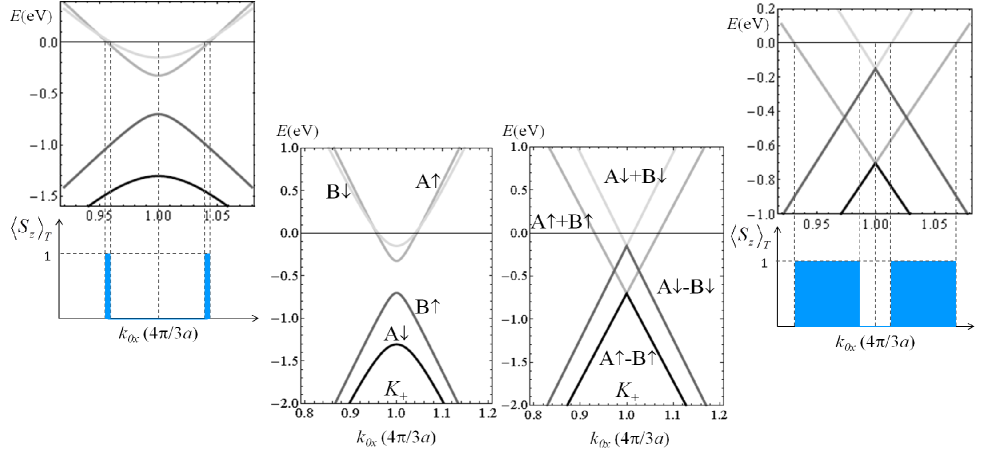
Figure 5: Band structure in the vicinity of the Dirac point for a monolayer of Co over graphene in the ATOP configuration (center-left) and the HCP configuration (center-right). The Fermi level (zero of energy) is indicated in both plots with a continuous line. In both cases the graphene layer is n-dopedKhomyakov . The eigenvectors corresponding to each band are indicated for both configurations. $k_{0x}$ is the adimensional wave vector in the $\hat{x}$ direction. In this plot $p_{y}=0$, $p_{x}=\hbar k_{x}-\hbar K_{\xi}$, and $\xi=+1$. The behavior of the total magnetization of graphene $\langle S_{z}\rangle_{T}$, given by the contribution of all bands, as a function of the wave vector $k_{x}=k_{0x}(4\pi/3a)$, for the ATOP configuration (upper-left) and the HCP configuration (upper-right). The shaded regions (blue online-only) indicate the zones in which the spin polarization is different from zero.

Although the previous simple tight binding model seems quite good, there are nevertheless some inconsistencies due to the truncation of higher order terms involving more complex couplings. We have used a separate spin splitting parameter $\delta_{2}$ to describe the coupling to $d_{xz},d_{yz}$ bands. For there to be a up spin magnetization, the average $\delta$ over all $d$ orbitals of the Co, should be negative. This is consistent with the top right relation (Eq.34) between DFT parametersMacdonald2013 and tight binding parameters. Nevertheless, the bottom right equation implies a positive $\delta$ value since $(\varepsilon_{p}-\varepsilon_{d})^{2}>\delta_{2}^{2}$, from an estimation using Hartree-Fock orbital energiesclementiroetti and $\delta_{2}$ from ref.Macdonald2013, . This cannot be corrected by including $d_{xy}$ and $d_{x^{2}-y^{2}}$ since these contributions add up with the same sign. In the DFT calculation the ratio between $\delta_{1}\sim-2.76$eV and $\delta_{2}\sim-1.083$eV is almost a factor of three but both have consistently a negative sign i.e. up (majority) spin is lower energy than down (minority) spin. All the rest of the parameters of the tight-binding have consistent values to DFT.

III.2 HCP bands

The continuum Hamiltonian in the vicinity of the K points for the HCP configuration is

$$H_{\rm HCP}(\mathbf{k})=\left(\begin{array}[]{cccc}-3\frac{\varepsilon+\delta_{2}}{\varepsilon^{2}-\delta_{2}^{2}}\widetilde{V}_{pd\pi}^{2}&0&-\frac{v}{\gamma_{0}}({-\gamma_{0}}+\frac{\varepsilon+\delta_{2}}{\varepsilon^{2}-\delta_{2}^{2}}\widetilde{V}_{pd\pi}^{2})p^{*}&0\\ 0&-3\frac{\varepsilon-\delta_{2}}{\varepsilon^{2}-\delta_{2}^{2}}\widetilde{V}_{pd\pi}^{2}&0&-\frac{v}{\gamma_{0}}({-\gamma_{0}}+\frac{\varepsilon-\delta_{2}}{\varepsilon^{2}-\delta_{2}^{2}}\widetilde{V}_{pd\pi}^{2})p^{*}\\ -\frac{v}{\gamma_{0}}({-\gamma_{0}}+\frac{\varepsilon+\delta_{2}}{\varepsilon^{2}-\delta_{2}^{2}}\widetilde{V}_{pd\pi}^{2})p&0&-3\frac{\varepsilon+\delta_{2}}{\varepsilon^{2}-\delta_{2}^{2}}\widetilde{V}_{pd\pi}^{2}&0\\ 0&-\frac{v}{\gamma_{0}}({-\gamma_{0}}+\frac{\varepsilon-\delta_{2}}{\varepsilon^{2}-\delta_{2}^{2}}\widetilde{V}_{pd\pi}^{2})p&0&-3\frac{\varepsilon-\delta_{2}}{\varepsilon^{2}-\delta_{2}^{2}}\widetilde{V}_{pd\pi}^{2}\end{array}\right),$$ (38)

where $p=\xi p_{x}+ip_{y}$, $p^{*}=\xi p_{x}-ip_{y}$ and $\varepsilon=\varepsilon_{p}-\varepsilon_{d}$. This Hamiltonian can be written as:

$$H_{\rm HCP}(\mathbf{k})=\left(\begin{array}[]{cccc}-\mu^{\prime}-h^{\prime}_{z0}&0&-\frac{v}{\gamma_{0}}({-\gamma_{0}}-h^{\prime}_{0x}-h^{\prime}_{zx})p^{*}&0\\ 0&-\mu^{\prime}+h^{\prime}_{z0}&0&-\frac{v}{\gamma_{0}}({-\gamma_{0}}-h^{\prime}_{0x}+h^{\prime}_{zx})p^{*}\\ -\frac{v}{\gamma_{0}}({-\gamma_{0}}-h^{\prime}_{0x}-h^{\prime}_{zx})p&0&-\mu^{\prime}-h^{\prime}_{z0}&0\\ 0&-\frac{v}{\gamma_{0}}({-\gamma_{0}}-h^{\prime}_{0x}+h^{\prime}_{zx})p&0&-\mu^{\prime}+h^{\prime}_{z0}\end{array}\right).$$ (39)

In order to estimate the coefficients $\mu^{\prime}$, $h_{z0}^{\prime}$, $h_{0x}^{\prime}$ and $h_{zx}^{\prime}$, of this Hamiltonian, we refer to the coupling of the B site in the ATOP configuration which was parameterized by DFT. Comparing equations (34), (38) and (39) we arrive at the values

$$\begin{split}\mu^{\prime}=-(\mu+h_{0z})=0.427~{}{\rm eV},\\ h_{z0}^{\prime}=\frac{h_{z0}-h_{zz}}{2}=0.276~{}{\rm eV},\\ \end{split}\quad\begin{split}h_{0x}^{\prime}=-\frac{\mu^{\prime}}{3}=-0.142~{}{\rm eV},\\ h_{zx}^{\prime}=-\frac{h_{z0}^{\prime}}{3}=-0.092~{}{\rm eV}.\end{split}$$ (40)

Diagonalization of the Hamiltonian $H_{\rm HCP}(\mathbf{k})$ gives the eigenvalues

$$\begin{split}\epsilon_{v}(\mathbf{k})&=-\mu^{\prime}+s_{z}h^{\prime}_{z0}+\frac{v\hbar}{\gamma_{0}}({-\gamma_{0}}-h^{\prime}_{0x}+s_{z}h^{\prime}_{zx})|\mathbf{k}|,\\ \epsilon_{c}(\mathbf{k})&=-\mu^{\prime}+s_{z}h^{\prime}_{z0}-\frac{v\hbar}{\gamma_{0}}({-\gamma_{0}}-h^{\prime}_{0x}+s_{z}h^{\prime}_{zx})|\mathbf{k}|.\end{split}$$ (41)

where $s_{z}$ are the eigenvalues of $S_{z}$ and correspond to the two possible spin orientations. In contrast to the ATOP configuration, here the dispersion is linear with a modified velocity ${\tilde{v}}_{F}={v}({-\gamma_{0}}-h^{\prime}_{0x}+s_{z}h^{\prime}_{zx})/\gamma_{0}$. Of course, corrections to velocities are one order of magnitude smaller that the pristine graphene values (see Eqs. 40).

One can diagonalize the Hamiltonian $H_{\rm HCP}(\mathbf{k})$ in the basis

$$\left(\begin{array}[]{c}A\uparrow\\ A\downarrow\\ B\uparrow\\ B\downarrow\end{array}\right) = \frac{1}{\sqrt{2}}\left(\begin{array}[]{c}0\\ 1\\ 0\\ \xi e^{i\xi\phi_{k}}\end{array}\right),\frac{1}{\sqrt{2}}\left(\begin{array}[]{c}1\\ 0\\ \xi e^{i\xi\phi_{k}}\\ 0\end{array}\right),\frac{1}{\sqrt{2}}\left(\begin{array}[]{c}0\\ 1\\ 0\\ -\xi e^{i\xi\phi_{k}}\end{array}\right),\frac{1}{\sqrt{2}}\left(\begin{array}[]{c}1\\ 0\\ -\xi e^{i\xi\phi_{k}}\\ 0\end{array}\right),$$ (62)

where $\phi_{k}=\arctan(p_{y}/p_{x})$. Given that in Eq. (38) we have other non diagonal terms besides the bare graphene terms, and therefore we have other $\mathbf{k}$ dependent terms, we cannot make a useful analysis at $\mathbf{k}=0$ as in the ATOP case. The diagonal Hamiltonian for $\mathbf{k}\neq 0$ close to $K_{\xi}$ is:

$$\begin{split}H_{\rm HCP}(\mathbf{k})&=-\mu^{\prime}\left(\begin{array}[]{cccc}{}_{A\uparrow+B\uparrow}&{}_{A\downarrow+B\downarrow}&{}_{A\uparrow-B\uparrow}&{}_{A\downarrow-B\downarrow}\\ 1&0&0&0\\ 0&1&0&0\\ 0&0&1&0\\ 0&0&0&1\end{array}\right)+\frac{v\hbar}{\gamma_{0}}|\mathbf{k}|(h^{\prime}_{0x}+\gamma_{0})\left(\begin{array}[]{cccc}{}_{A\uparrow+B\uparrow}&{}_{A\downarrow+B\downarrow}&{}_{A\uparrow-B\uparrow}&{}_{A\downarrow-B\downarrow}\\ 1&0&0&0\\ 0&1&0&0\\ 0&0&-1&0\\ 0&0&0&-1\end{array}\right)\\ &-h^{\prime}_{z0}\left(\begin{array}[]{cccc}{}_{A\uparrow+B\uparrow}&{}_{A\downarrow+B\downarrow}&{}_{A\uparrow-B\uparrow}&{}_{A\downarrow-B\downarrow}\\ 1&0&0&0\\ 0&-1&0&0\\ 0&0&1&0\\ 0&0&0&-1\end{array}\right)+\frac{v\hbar}{\gamma_{0}}|\mathbf{k}|h^{\prime}_{zx}\left(\begin{array}[]{cccc}{}_{A\uparrow+B\uparrow}&{}_{A\downarrow+B\downarrow}&{}_{A\uparrow-B\uparrow}&{}_{A\downarrow-B\downarrow}\\ 1&0&0&0\\ 0&-1&0&0\\ 0&0&-1&0\\ 0&0&0&1\end{array}\right)\\ &=-\mu^{\prime}\mathbbm{1}_{\sigma}\mathbbm{1}_{s}+\frac{v\hbar}{\gamma_{0}}|\mathbf{k}|(h_{0x}^{\prime}+\gamma_{0})\widetilde{\sigma}_{z}\mathbbm{1}_{s}-h_{z0}^{\prime}\mathbbm{1}_{\sigma}S_{z}+\frac{v\hbar}{\gamma_{0}}|\mathbf{k}|h_{zx}^{\prime}\widetilde{\sigma}_{z}S_{z},\end{split}$$ (63)

where $\widetilde{\sigma}_{z}$ is the pseudospin matrix in the basis of Eq. (62). Within this basis, the interpretation of the terms is not so straight-forward as for the ATOP configuration. However, one can see that the first term also shifts the site energy, with a chemical potential $\mu^{\prime}=0.427~{}$eV, that represents a transfer of electrons from Co/Ni to graphene. We can see this effect in Fig. 5 (right panels). For the second term we have $h_{0x}^{\prime}=-0.142~{}$eV, and looking at Eq. (63), we see that the states $A\uparrow-B\uparrow$ and $A\downarrow-B\downarrow$ are equally favorable, indicating symmetry between the sublattices A and B. This is because in the sublattice symmetric configuration, both A and B, are at the HCP sites of Co (Figs. 1 and 3).

The magnetic order of graphene, with respect to Co magnetic order, is determined by the eigenvalue of lowest energy and its corresponding eigenvector in Eq. (63). Given that $h_{z0}^{\prime}=0.276~{}$eV and $h_{zx}^{\prime}=-0.092~{}$eV, this state corresponds to $|A\uparrow-B\uparrow\rangle$. Using this state, with $k_{y}=0$ and $\xi=1$, we have

$$\langle S_{z}\rangle = \langle A\uparrow{-}B\uparrow|\mathbbm{1}_{\sigma}S_{z}|A\uparrow{-}B\uparrow\rangle$$ (73)

$$= \frac{1}{2}\left(\begin{array}[]{c c c c}1&0&{-}1&0\end{array}\right)\left(\begin{array}[]{c c c c}1&0&0&0\\ 0&-1&0&0\\ 0&0&1&0\\ 0&0&0&-1\end{array}\right)\left(\begin{array}[]{c}1\\ 0\\ {-}1\\ 0\end{array}\right)=1,$$

so every band has a full spin polarization in either of the two spin orientations as depicted in right-hand panel of Fig.5.

The coupling of the spin and kinetic energy (see last term in Eq.63) induces a striking behavior which mimicks a spin-orbit coupling induced by the bias current and the magnetism of the Co. In the sense of equilibrium/persistent currentsBolivar , at ${k}=0$ all bands have occupation below the Fermi energy, thus the spin polarization is zero at both K points. As $k_{x}$ increases e.g. in the positive direction, (see Fig. 5 upper-right panel) one of the bands emerges above the Fermi level and we have a net polarization which is up spin. A range of $k_{x}$ values preserves this polarization until a second band emerges from the Fermi sea, then the polarization returns to zero. The same behavior occurs in the opposite $k_{x}$ direction. This behavior is also borne out from the ATOP configuration but within a smaller wave-vector range (see Fig. 5 upper-left panel) in the vicinity of the K point. Note that this term is not derived from the atomic SOI (as is the case for both the intrinsic and Rashba interactions) but is purely parameterized by the spin-splitting energy of the Co and the wave-vector deviation from the K point. As can be seen from Eqs.34 and 40, if the spin-splitting energy $\delta_{1,2}$ vanishes, this term does not appear.

Following the lowest energy occupied states, the system is ferromagnetic in the vicinity of $k=0$. At the K point we have degenerate bands with the same spin orientation as the Co layer, nevertheless, driving a current by means of an external electric field in the graphene plane, one can tune the $k_{x}$ vector so that two oppositely oriented bands are the lowest occupied bands, making the magnetization ground state zero. So we have magnetic state switching controlled by the charge current on the graphene layer.

Various scenarios of interest can be explored by using, as proposed in ref. Macdonald2013, , a Cu surface so as to sandwich the graphene layer between Co and Cu. The Cu surface will serve to control the Fermi level and access differently polarized magnetization states as a function of gate voltage and charge current.

IV Conclusions

We have derived, within the perturbative tight-binding approximation, the spectral signatures of two Co-graphene registries, the ATOP (one Co atom atop of each A carbon atom) configuration and the HCP (Co at the centers of the hexagonal cells of graphene). Each registry produces a very different spectrum: a) The ATOP configuration generates a gap in pristine graphene with spin dependent electron heavy and light effective masses for both the conduction and valence bands that are tunable controlling orbital overlaps. As found by DFT, the graphene layer becomes almost perfectly antiferromagnetic with down spin orientations at sublattice A and up spin favoured orientation at sublattice B. b) The HCP configuration preserves the linear dispersion of graphene, with a small modification of the fermion velocities. The resulting linear dispersions shift in energy according to the spin orientation favoured on the sublattices. For this configuration, ferromagnetic order is preferred and it is parallel to the Co polarization. We have suggested ways to manipulate the magnetic state of the surface by applying a gate voltage (in the work function regime) and by driving a current through the system. There is peculiar coupling between spin and electron momentum induced by the magnetic state of the Co. It amounts to a spin-orbit coupling induced by the driving current. This feature is worth while exploring in the future for both its transport and topological implications in graphene nanoribbons.

Using Co and Ni interchangeably in this work is a good approximation as can be judged from detailed DFT calculationsDFTReference . Nevertheless, there are some quantitative differences in the amount of charge transfer and the magnetic moment on the graphene mainly induced by slight changes in the bonding lengths both in the graphene and the interface layer involved. For the ATOP configuration the charge transfers per carbon atom are almost identical between Co and Ni, but the induced magnetization can be two times higher for Ni for small number of layers of the metal. Also the gap induced in the ATOP configuration can be manipulated slightly by changing the number of layers without changing the qualitative picture. It remains to be seen what the corresponding effects are from the HCP, configuration.

Appendix A Direction cosine sums

The summation $\sum_{m,l=1}^{3}[\hat{n}_{lx}\hat{n}_{lmx}+\hat{n}_{ly}^{2}\hat{n}_{lmy}]$ is performed as follows: Performing first the sum over $l$ i.e. over the Co/Ni atoms $l=1,2,3$ as can be seen in Fig. 4, $n_{1x}=0$, because there is no overlap between A and Co in $\hat{x}$ for $l=1$. The other terms are $n_{1y}=-1$, $n_{2y}=n_{3y}=1/2$ and $n_{2x}=-\sqrt{3}/2$ $n_{3x}=\sqrt{3}/2$. Therefore

$${\sum_{l=1}^{3}\sum_{m=1}^{3}(\hat{n}_{lx}\hat{n}_{lmx}+\hat{n}_{ly}\hat{n}_{lmy})}=$$

$$\sum_{m=1}^{3}[-n_{1my}+\frac{n_{2my}+n_{3my}}{2}+\frac{\sqrt{3}}{2}(n_{3mx}-n_{2mx})].$$

Now performing the remaining sum, for $m=1$ only the cobalts $l=2$ and $l=3$ intervene, so $n_{11y}=0$, $n_{21y}=n_{31y}=1/2$ and $n_{21x}=\sqrt{3}/2$, $n_{31x}=-\sqrt{3}/2$. Doing the sum for $m=1$ we have

$$m=1:\Big{[}-0+\frac{1/2+1/2}{2}+\frac{\sqrt{3}}{2}\Big{(}-\frac{\sqrt{3}}{2}-\frac{\sqrt{3}}{2}\Big{)}\Big{]}=-1.$$

For $m=2$ only the Co/Ni $l=2$ and $l=1$ intervene, so $n_{12y}=1/2$, $n_{22y}=-1$ ,$n_{32y}=0$, $n_{22x}=0$ and $n_{32x}=0$. Doing the sum for $m=2$ one obtains

$$m=2:\Big{[}-\frac{1}{2}+\frac{-1+0}{2}+\frac{\sqrt{3}}{2}\Big{(}0-0\Big{)}\Big{]}=-1.$$

Finally, for $m=3$ the intervening Co/Ni are $l=1$ and $l=3$, so $n_{13y}=1/2$, $n_{23y}=0$, $n_{33y}=-1$, $n_{23x}=0$ and $n_{33x}=0$. The sum for $m=3$ is then

$$m=3:\Big{[}-\frac{1}{2}+\frac{0-1}{2}+\frac{\sqrt{3}}{2}\Big{(}0-0\Big{)}\Big{]}=-1.$$

So in spite of the complicated combination of direction cosines, all the matrix overlaps are equivalent.

Appendix B Parameter values of the ATOP Hamiltonian

From Eq. 34, with $\varepsilon=\varepsilon_{p}-\varepsilon_{d}$, one obtains

$$\mu = -\frac{\varepsilon}{2}\left(\frac{V^{2}_{pdz}}{\varepsilon^{2}-\delta_{1}^{2}}+3\frac{\widetilde{V}^{2}_{pd\pi}}{\varepsilon^{2}-\delta_{2}^{2}}\right),$$ (76)

$$h_{0z} = \frac{\varepsilon}{2}\left(\frac{V^{2}_{pdz}}{\varepsilon^{2}-\delta_{1}^{2}}-3\frac{\widetilde{V}^{2}_{pd\pi}}{\varepsilon^{2}-\delta_{2}^{2}}\right),$$ (77)

$$h_{z0} = \frac{\delta_{1}V^{2}_{pdz}}{\varepsilon^{2}-\delta_{1}^{2}}+3\frac{\delta_{2}\widetilde{V}^{2}_{pd\pi}}{\varepsilon^{2}-\delta_{2}^{2}},$$ (78)

$$h_{zz} = \frac{\delta_{1}V^{2}_{pdz}}{\varepsilon^{2}-\delta_{1}^{2}}-3\frac{\delta_{2}\widetilde{V}^{2}_{pd\pi}}{\varepsilon^{2}-\delta_{2}^{2}}.$$ (79)

References

• (1) K. S. Novoselov, V. I. Falko, L. Colombo, P. R. Gellert, M. G. Schwab, K. Kim, Nature 490, 192 (2012).
• (2) L. Song et al., Nano Lett. 10, 3209 (2010).
• (3) H. Kazi, Y. Cao, I. Tanabe, M. S. Driver, P. A. Dowben and J. A. Kelber, Mater. Res. Express 1, 035601 (2014).
• (4) D. Marchenko, A. Varykhalov, M. R. Scholz, G. Bihlmayer, E. I. Rashba, A. Rybkin, A. M. Shikin, and O. Rader, Nat. Comm. 3, 1232 (2012).
• (5) Z. Wang, C. Tang, R. Sachs, Y. Barlas, and J. Shi, Phys. Rev. Lett. 114, 016603 (2015).
• (6) S. Ostovar pour et al. Nature Chem. 7, 591 (2015).
• (7) S. J. Gong et al, New J. Phys. 12, 103040 (2010). S. J. Gong et al, Appl. Phys. Lett. 100, 122410 (2012); C. D. Porter and D. Stroud, Phys. Rev. B 85, 235452 (2012).
• (8) H. Chen, Q. Niu, Z. Zhang, and A. H. MacDonald, Phys. Rev. B 87, 144410 (2013).
• (9) M. A. H. Vozmediano, M. P. Lopéz-Sancho, T. Stauber, and F. Guinea, Phys. Rev. B 72, 155121 (2005).
• (10) L. Brey, Phys. Rev. B 92, 235444 (2015).
• (11) J. Balakrishnan, G. Kok Wai Koon, M. Jaiswal, A. H. Castro Neto, and B. Ozyilmaz, Nat. Phys. 9, 284 (2013).
• (12) J. C. Slater, and G. F. Koster, Phys. Rev. 94, 1498 (1954).
• (13) S. Konschuh, M. Gmitra, and J. Fabian, Phys. Rev. B 82, 245412 (2010).
• (14) H. M. Pastawski, and E. Medina, Rev. Mex. Fís. 47 Supp 1, 1 (2001); S. Varela, V. Mujica, and E. Medina, Phys. Rev. B 93, 155436 (2016).
• (15) G. Giovannetti, P. A. Khomyakov, G. Brocks, V. M. Karpan, J. van den Brink, and P. J. Kelly, Phys. Rev. Lett. 101, 026803 (2008).
• (16) P. A. Khomyakov, G. Giovannetti, P. C. Rusu, G. Brocks, J. van den Brink, and P. J. Kelly, Phys. Rev. B 79, 195425 (2009).
• (17) E. Clementi, and C. Roetti, Atomic Data and Nuclear Data Tables 14, 177 (1974).
• (18) N. Bolívar, E. Medina, and B. Berche, Phys. Rev. B 89, 125413 (2014).
• (19) T. Abtew, B.-C. Shih, S. Banerjee, and P. Zhang, Nanoscale 5, 1902 (2013).
• (20) E. McCann, and M. Koshino, Rep. Prog. Phys. 76, 056503 (2013).