Integrated and Resolved Dust Attenuation in Clumpy Star-Forming Galaxies at 0.07 < $z$ < 0.14

Abstract

Dust attenuation in galaxies has been extensively studied nearby, however, there are still many unknowns regarding attenuation in distant galaxies. We contribute to this effort using observations of star-forming galaxies in the redshift range z = 0.05-0.15 from the DYNAMO survey (Green et al., 2014). Highly star-forming DYNAMO galaxies share many similar attributes to clumpy, star-forming galaxies at high redshift. Considering integrated Sloan Digital Sky Survey (York et al., 2000) observations, trends between attenuation and other galaxy properties for DYNAMO galaxies are well matched to star-forming galaxies at high redshift. Integrated gas attenuations of DYNAMO galaxies are 0.2-2.0 mags in the V-band, and the ratio of $E(B-V)_{stars}$ and $E(B-V)_{gas}$ is 0.78-0.08 (compared to 0.44 at low redshift, Calzetti, 1997). Four highly star-forming DYNAMO galaxies were observed at H$\alpha$ using the Hubble Space Telescope and at Pa$\alpha$ using integral field spectroscopy at Keck. The latter achieve similar resolution ($\sim$0.8-1 kpc) to our HST imaging using adaptive optics, providing resolved observations of gas attenuations of these galaxies on sub-kpc scales. We find < 1.0 mag of variation in attenuation (at H$\alpha$) from clump to clump, with no evidence of highly attenuated star formation. Attenuations are in the range 0.3-2.2 mags in the V band, consistent with attenuations of low redshift star-forming galaxies. The small spatial variation on attenuation suggests that a majority of the star-formation activity in these four galaxies occurs in relatively unobscured regions and, thus, star-formation is well characterised by our H$\alpha$ observations.

1 Introduction

Understanding dust attenuation in galaxies is an essential ingredient in studies of galaxy formation and evolution. In the current paradigm, the relationship between star-formation rate (SFR) and stellar mass (the star-forming “main sequence”, e.g. Brinchmann et al., 2004; Elbaz et al., 2007; Whitaker et al., 2012) is an important tool, however, it is highly dependent on prescriptions for dust attenuation due to the strong influence of dust on various SFR indicators. An accurate description of the effects of dust during the peak of cosmic star-formation ($1<z<3$, Lilly et al., 1996; Madau et al., 1998; Reddy & Steidel, 2009; Cucciati et al., 2012) remains elusive due to observational constraints. Star-forming galaxies at these epochs are found to form stars much more rapidly than local galaxies, and it is unclear whether or not local attenuation relations (see Calzetti, 2001, for a review) can be applied (Price et al., 2014; Reddy et al., 2015). The assumption of a screen-like dust geometry, as well as the relationship between attenuation and mass (Garn & Best, 2010), may affect the normalisation of the star-forming main-sequence, both of which are difficult to study at high redshift.

The flux of the H$\alpha$ emission line in the optical is a standard indicator of the SFR of a given galaxy (Kennicutt & Evans, 2012) and, although it can be significantly attenuated by dust, it is commonly used to study star-formation at both low and high redshift. For an ideal correction, one would measure the attenuation for the gaseous component by comparing the H$\alpha$ to H$\beta$ recombination line ratio ($R($H$\alpha$,H$\beta)$, the Balmer decrement, Berman, 1936; Mathis, 1983) to the intrinsic value for typical star-forming regions ($R($H$\alpha$,H$\beta)_{int}=2.87$, from Case B recombination Hummer & Storey, 1987; Osterbrock, 1989). By definition, this indicator is directly associated with line emission originating from star-forming regions. Detecting both H$\alpha$ and H$\beta$ at $z>1$ for single galaxies, however, is difficult due to the faintness of H$\beta$ (particularly at high attenuation, Erb et al., 2006; Yoshikawa et al., 2010; Domínguez et al., 2013; Price et al., 2014). Furthermore using current instruments this may require observations in multiple bands (e.g. Kashino et al., 2013). For these reasons, the attenuation of the stellar light may be measured first, often through fitting of the spectral energy distribution (SED), with the attenuation of H$\alpha$ then estimated based on the local relation for starburst galaxies: $E(B-V)_{stars}=0.44\times E(B-V)_{gas}$ (Calzetti, 1997; Yoshikawa et al., 2010; Mancini et al., 2011). The universality of this relation is far from certain, particularly at high redshift (Wild et al., 2011; Kashino et al., 2013; Wuyts et al., 2013; Price et al., 2014; Reddy et al., 2015; Battisti et al., 2016; Puglisi et al., 2016). Furthermore, Kreckel et al. (2013) show that the applicability of the local relation can vary significantly within individual galaxies. Thus further investigation of stellar versus ionized gas attenuation is warranted.

The work of Kreckel et al. (2013) shows that studying attenuation in external galaxies is further complicated by dust geometry, which is often only broadly characterised due to the integrated nature of many observations. Within the Milky Way, variations in extinction from 0 to 30 magnitudes have been observed (Cambrésy et al., 2011) while integrated attenuations of face-on disk galaxies at $z<0.8$ typically fall in the narrow range of $\sim 0.5-2.0$ magnitudes in the B-band (e.g. Keel & White, 2001; Matthews & Wood, 2001; Takeuchi et al., 2005b; Cortese et al., 2008). The difference in measurements of the Milky Way versus external galaxies highlights the limitations of integrated attenuation measurements. A solution to this is offered by resolved observations such as those of Calzetti et al. (1997) who target NGC 5253 finding variation in attenuation from 0 to 9 mag. With the recent proliferation of integral field spectroscopy (IFS) resolved observations of attenuation such as these are becoming more commonplace (e.g. Bedregal et al., 2009; Kreckel et al., 2013; Piqueras López et al., 2013).

The effects of large-scale dust geometry will likely play an important role in highly star-forming galaxies at high redshift hosting massive star-forming clumps (Wright et al., 2009; Förster-Schreiber et al., 2009; Wisnioski et al., 2011; Epinat et al., 2012; Swinbank et al., 2012). Although the exact definition of a star-forming clump varies somewhat between authors, in general this terminology refers to individual, large-scale, star-forming regions typically identified by their strong emission lines. Currently little is known regarding clump-to-clump variations in attenuation although one study by Genzel et al. (2013) infers possible attenuations of up to 50 mags, albeit with uncertain assumptions regarding dust geometry, based on molecular gas observations. Locally, the most highly attenuated galaxies are highly star-forming, infrared (IR) bright galaxies known as luminous (and ultraluminous) star-forming galaxies (LIRGS/ULIRGS see Sanders & Mirabel, 1996, for a review). Integrated attenuations of these objects are measured to be $\sim$3-5.5 mag in the $V$-band (e.g. Calzetti et al., 2005; Alonso-Herrero et al., 2006). These values fail to give the full picture, however, as they assume simple dust geometries while resolved observations reveal pixel to pixel variation of $\sim$1-20 mag (e.g. Piqueras López et al., 2013). The counterpart at high redshift are so called submillimeter galaxies (SMGs; see Blain et al., 2002, for a review) that radiate a very large fraction of their energy in the IR, possibly implying that they contain enough dust to be nearly optically thick. Current results suggest galaxies on the high redshift star forming main sequence are significantly less attenuated, though, with values closer to local main sequence galaxies (e.g. Price et al., 2014; Reddy et al., 2015). However, considering the results of Alonso-Herrero et al. (2006) and Piqueras López et al. (2013) for local ULIRGS, further study of dust geometry in clumpy, star-forming galaxies is necessary.

In this paper we highlight two important open questions regarding dust geometry in clumpy, high redshift galaxies. Are clumps a genuine morphological feature, or are variations in dust attenuation a large contributor to the appearance of these galaxies? And, if dust is highly variable spatially, will this strongly bias measurements of galaxy SFR at high redshift? Due to the difficulties in studying attenuation at high redshift highlighted above, studies of dust geometry using resolved IFS observations of extremely star-forming galaxies at low redshift may present a viable step forward.

Here we explore the spatially resolved attenuation properties of a unique sample of star-forming galaxies taken from the DYnamics of Newly Assembled Massive Objects survey (DYNAMO, Green et al., 2014). DYNAMO galaxies are drawn from the Sloan Digital Sky Survey Data Release 4 (SDSS DR4, York et al., 2000) and previous observations have shown highly star-forming DYNAMO galaxies to share many similar properties to clumpy galaxies at high redshift (Green et al., 2014; Bassett et al., 2014; Fisher et al., 2014; Obreschkow et al., 2015). Here we compare Hubble Space Telescope (HST) H$\alpha$ photometry and adaptive optics (AO) assisted infrared (IR) IFS of Paschen $\alpha$ (Pa$\alpha$) to study the spatially resolved gas attenuation in four clumpy, high SFR DYNAMO galaxies on $\sim 1$ kpc scales. Although kpc scale observations of clumpy galaxies at $z>1.5$ are possible using gravitational lensing and/or AO, obtaining such observations of both H$\alpha$ and H$\beta$ at these redshifts has to this point been infeasible. Thus, our study provides a necessary test of clump-to-clump variation in attenuation for turbulent, clumpy galaxies.

This paper is laid out as follows: in Section 2 we present the data sets used for both our integrated and resolved analyses, in Section 3 we present a brief analysis of the integrated stellar and gas attenuation properties of DYNAMO galaxies, in Section 4 we describe the analysis performed in producing resolved maps of attenuation for our subsample of four extreme DYNAMO galaxies, in Section 4.2 we present the results of our resolved attenuation analysis, in Section 5 we provide a discussion of all of our results, and in Section 6 we give a brief summary and itemise our conclusions. Throughout this work, we adopt a flat cosmology with $H_{0}=70$ km s^-1 Mpc^-1 and $\Omega_{M}=0.3$.

2 Samples and Data

2.1 DYNAMO: A Local Sample of High-$z$ Analogs

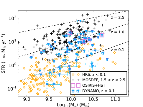
Figure 1: $M_{*}$ vs SFR (from H$\alpha$ luminosity) for 67 DYNAMO galaxies from Green et al. (2014) along with our two comparison samples. At low redshift we select late-type star-forming galaxies from the Herschel Reference Survey while the MOSDEF survey provides a sample of star-forming galaxies at $z>1.5$. We also plot the redshift evolution of the main-sequence of star-forming galaxies given by Whitaker et al. (2012) at $z$=0.1, 1.0, and 2.5. DYNAMO galaxies exhibit significant overlap between both samples, bridging the gap in star-formation properties from low to high redshifts. The four galaxies for which resolved observations are also presented in this paper are indicated by open purple squares.

DYNAMO galaxies were selected in two redshift bins chosen to avoid contamination of the H$\alpha$ emission line by common night sky emission lines. In both bins active galactic nuclei (AGN) have been excluded using the standard procedure of Baldwin, Phillips & Terlevich (1981, the “BPT diagram”) in order to focus on purely star-forming, line-emitting galaxies. Initial IFS observations revealed a number of galaxies with clumpy disk morphologies and turbulent kinematics (as indicated by a large gas velocity dispersion, $\sigma_{gas}$, Green et al., 2014) reminiscent of star-forming galaxies observed at $z>1$. Follow-up observations using IFS at the Gemini and Keck observatories have confirmed that this kinematic signature is not an artifact of resolution for a handful of DYNAMO disks at $z=0.1$ (Bassett et al., 2014, Oliva-Altamirano et al. in prep). Three DYNAMO galaxies have been securely detected in unresolved CO observations indicating gas fractions of up to 30% (measured for DYNAMO G 04-1 included in this work, Fisher et al., 2014). For these reasons a subset of highly star-forming DYNAMO galaxies represent the best-known sample at $z<0.2$ for studying star-formation processes more common at $z>1.5$.

The relatively wide range of properties for the DYNAMO sample is reflected in Figure 1 where we show the relationship between $M_{*}$ and SFR for DYNAMO galaxies. $M_{*}$ values are taken from the MPA-JHU VAC, and they are calculated using the population synthesis methods presented in Kauffmann et al. (2003a). SFR is calculated based on the spatially integrated H$\alpha$ luminosity from IFS observations presented in Green et al. (2014) with an attenuation correction based on the Balmer decrement from SDSS observations (Tremonti et al., 2004) and following the method of Calzetti (1997). The attenuation corrected H$\alpha$ luminosity is then convrted to SFR following calibration of Kennicutt (1998) modified for a Chabrier (2003) initial mass function. Here we compare DYNAMO galaxies with the $M_{*}$-SFR relationships for low redshift and high redshift star-forming galaxies. These redshift regimes are represented by the Herschel Reference Survey (HRS) of nearby star-forming galaxies (Boselli et al., 2010; Cortese et al., 2012b; Boselli et al., 2015) and the MOSFIRE Deep Evolution Field (MOSDEF) survey (Kriek et al., 2015; Reddy et al., 2015, see Section 2.4 for further description of the MOSDEF sample) respectively. Overplotted as dashed lines are fits of the main sequence of star-forming galaxies (e.g Brinchmann et al., 2004) taken from Whitaker et al. (2012) at redshifts 0.1, 1.0 and 2.5. DYNAMO galaxies are found to exhibit a large scatter in SFR at fixed $M_{*}$ with galaxies typical of the local and $z>1.0$ main sequence represented. We indicate galaxies for which resolved attenuations are explored in this work with open purple squares. These four galaxies are found to have SFR and $M_{*}$ roughly consistent with the $z=1.0$ main sequence.

2.2 Unresolved Sample

We begin this work by briefly investigating the integrated attenuations of the full sample of DYNAMO galaxies presented by Green et al. (2014) in order to provide context for our resolved observations. These 67 galaxies make up our unresolved attenuations sample. We show the relationship between $M_{*}$ and SFR for these 67 galaxies as inverted blue triangles in Figure 1. This shows that DYNAMO galaxies exhibit a wide range in star-formation properties.

Of particular interest here is the comparison between attenuations suffered by the stellar and ionized gas components of DYNAMO galaxies. If highly star-forming DYNAMO galaxies are true analogs of high redshift galaxies, they may exhibit a similar departure from local galaxies that show roughly two times more attenuation for ionised gas (Calzetti, 1997; Price et al., 2014; Reddy et al., 2015, e.g.). Our method of calculating integrated attenuations based on the Max Planck Institute for Astrophysics and Johns Hopkins University Value Added Catalog (MPA-JHU VAC; Kauffmann et al., 2003a; Tremonti et al., 2004) is described in Section 3.1.

2.3 Four Resolved Attenuations Galaxies

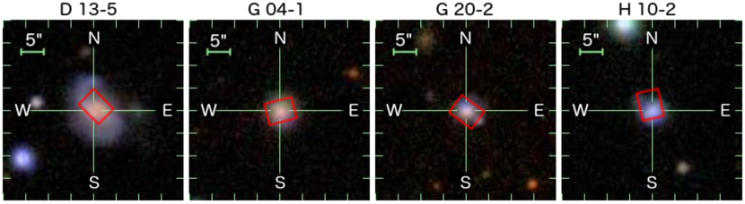
Figure 2: SDSS postage stamps of the four galaxies in our resolved attenuation sample. In each panel a scale bar indicating a size of 5$\aas@@fstack{\prime\prime}$0 is shown in green and the approximate field of view of our OSIRIS observations is shown as a red rectangle. Note that the field of view of our HST observations is significantly larger than the postage stamps pictured here.

Galaxies in our resolved attenuations sample are selected from the overlap of two separate DYNAMO programs, a HST photometric program targeting H$\alpha$ in 10 galaxies (see Section 2.3.1) and an AO assisted IR IFS program using the OH-Suppressing Infrared Integral field Spectrograph (OSIRIS, Larkin et al., 2006) at the Keck observatory targeting Pa$\alpha$ in 15 galaxies (see Section 2.3.2). These programs were designed to explore the properties of analogs to high redshift, clumpy galaxies, thus both selections include primarily highly star-forming DYNAMO galaxies. The primary goals of our H$\alpha$ and Pa$\alpha$ programs were to study the size-luminosity relation for clumps in DYNAMO galaxies (Fisher et al., 2016) and sub-kpc kinematics of DYNAMO galaxies (Oliva-Altamirano et al. in prep.) respectively.

Galaxies observed in each program were subject to different constraints, therefore only four galaxies, D 13-5, G 04-1, G 20-2, and H 10-2, comprise the overlap between our HST and OSIRIS programs. These four DYNAMO galaxies were previously classified as rotating disks by Green et al. (2014), and they exhibit large velocity H$\alpha$ velocity dispersion (45-60 km s^-1), and form stars rapidly (SFR$\sim$15-40 M_⊙ yr^-1). Integrated galaxy properties for this subsample are summarised in Table 1 and SDSS postage stamps are shown in Figure 2 with red rectangles indicating the approximate field of view of our OSIRIS observations.

ID z $\mathcal{M}_{*}$ SFR_Hα $\sigma_{gas}$ PSF Scale Type ($10^{9}$ M_⊙) (M_⊙yr^-1) (km s^-1) (kpc) D 13-5 0.075 53.84 12.31$\pm$0.86 46 0.21 (0.85) disk G 04-1 0.129 64.74 20.00$\pm$2.17 50 0.35 (1.39) disk G 20-2 0.141 21.56 10.80$\pm$0.66 45 0.38 (1.50) disk H 10-2 0.149 9.5 25.35$\pm$2.68 59 0.39 (1.57) merger

Table 1: Resolved Attenuation Sample: Previous DYNAMO Observations

Galaxies D 13-5, G 04-1, and G 20-2 are characterised by undisturbed continuum morphologies and smooth, disk-like rotation. Two of these, G 04-1 and G 20-2, are in the $z\sim 0.1$ and high H$\alpha$ flux bins of the original DYNAMO sample and as such their angular sizes and fluxes are well suited to observation with OSIRIS. We also note that the stellar versus ionized gas kinematics in galaxies G 04-1 and G 20-2 were the subject of another recent work (Bassett et al., 2014) finding these galaxies to be consistent with rotating disks using higher resolution IFS observations from the Gemini Observatory. The third disk-like galaxy, D 13-5, is at a lower redshift and we therefore primarily cover only the central most regions of this galaxy, missing flux at large radii.

The fourth galaxy in our sample, H 10-2, was originally identified as an extremely H$\alpha$ luminous galaxy with disk-like rotation from our initial observations. Deep optical IFS using Gemini MultiObject Spectrometer (GMOS) at The Gemini Observatory (see Bassett et al., 2014, for description of GMOS observations) revealed a second component rotating at 90 degrees relative to the previously identified kinematic axis. These kinematic components correspond to two significant peaks in continuum emission leading us to reclassify this galaxy as an ongoing merger. Regardless, we include this object in our analysis, as it is valuable as a comparison to our disk sample.

2.3.1 H$\alpha$ Photometric Observations

Our H$\alpha$ photometry was collected using HST Advanced Camera for Surveys Wide-Field Camera (ACS/WFC) FR647M (Proposal ID 12977, PI: Damjanov). Observations were performed using the FR716N and FR782N ramp filters, which are equivalent to tunable narrow-width pass band filters, targeting H$\alpha$ emission with a 2% bandwidth. Continuum subtraction is achieved using observations in the associated continuum filter, FR647M. Integration times for our H$\alpha$ and continuum observations are 45 min and 15 min respectively. The typical HST pipeline is used to reduce images for analysis. The full HST sample of 10 detected galaxies is presented in Fisher et al. (2016).

2.3.2 Infrared IFS Observations and Reduction

Pa$\alpha$ data comes from IFS observations using the OSIRIS instrument at the Keck Observatory. OSIRIS is a lenslet array spectrograph with a $2048\times 2048$ Hawaii-2 detector and spectral resolution R $\sim$ 3000 in the 100 mas spatial scale. We perform our observations with the aid of natural guide star (NGS) or laser guide star (LGS) AO systems at Keck (Wizinowich et al., 2006; van Dam et al., 2006). Galaxy D 13-5 was observed on Keck I in July 2012 using NGS-AO ($\sim$0$\aas@@fstack{\prime\prime}$85 optical seeing), G 20-2 was also observed in July 2012 on Keck I with the aid of LGS-AO ($\sim$0$\aas@@fstack{\prime\prime}$65 optical seeing), G 04-1 was observed on Keck I in September 2012 using LGS-AO ($\sim$0$\aas@@fstack{\prime\prime}$60 optical seeing), and finally galaxy H 10-2 was observed at Keck II in March 2010 using LGS-AO. Note that while the AO point spread function (PSF) has a core that is significantly narrower than the seeing (typically $\sim$0$\aas@@fstack{\prime\prime}$15 in our observations), the shape and width are known to vary significantly both from night to night as well as within a single night of observations. Discussion of the AO PSF is revisited in Section 4.1.2. We will present the analysis of high-resolution Pa alpha kinematic properties for star-forming clumps in the full sample of 15 DYNAMO galaxies observed with OSIRIS in the upcoming publication (Oliva-Altamirano et al. in prep)

The standard observing procedure was as follows. We first acquired the tip-tilt star and applied the optimal position angle of OSIRIS to position the star within the unvignetted field-of-view of the LGS-AO system. Short, 60s, integrations were taken on the star for calculations of the PSF and to centre the star in the field for the target offsets. Multiple positions for science observations were dithered by 0$\aas@@fstack{\prime\prime}$05 around the base positions in each exposure to remove bad pixels and cosmic ray contamination. Sky frames were taken completely offset from the object as the galaxies fill the whole field of view of OSIRIS. All galaxies were observed in the 100mas scale.

Data reduction was completed using the OSIRIS data reduction pipeline version 2.3, and custom IDL routines developed for faint emission-line spectra. The pipeline removes crosstalk, detector glitches, and cosmic rays before it mosaics individual exposures and assembles a reduced data cube with two spatial dimensions and one spectral dimension. First order sky subtraction was achieved by the spatial nodding on the sky. Further sky subtraction was applied using custom IDL routines that employ the methods of Davies (2007). We initially perform a spectrophotometric flux calibration to our OSIRIS IFS observations by comparing standard star observations to a synthetic spectrum of Vega, however, strong variability in the AO PSF over a night results in large systematic uncertainties on the order of $\sim$30% (when comparing observed OSIRIS continuum flux densities to catalog values from 2MASS), comparable to other works using OSIRIS (e.g. Law et al., 2009). For this reason, we subsequently adjust the integrated flux of Pa$\alpha$ for each galaxy to match the expected flux based on the SDSS Balmer decrement. This is described further in Section 4.1.4 and the correction varies by a factor of 1.07 for H 10-2 to 2.61 for D 13-5.

2.3.3 Ancillary IFS Data

G 20-2 [OIII]/H$\beta$: We also explore variations in the ionization state of the gas in galaxy G 20-2 using optical GMOS-IFS observations of H$\beta$ and [OIII] (5007 Å). A full description of the observations and data reduction can be found in Bassett et al. (2014). Using these observations we can recover some information on the ionization state of the gas by comparing the strength of the Balmer emission to that of the forbidden transition of oxygen. In particular, we explore the possibility of a low-luminosity AGN that may explain irregularity in the measured ionized gas attenuation in the central regions (see Section 4.2).

Flux calibration is achieved by matching a spectrum summed in an approximation of the SDSS fibre footprint on our IFS datacube to the observed SDSS spectrum in the same wavelength range. We then map both the [OIII] and H$\beta$ emission lines as described in Section 4.1.1. We note that because they are separated by < 150 Å mapping the ratio of these two lines does not depend significantly on the absolute accuracy of this calibration. A map of log${}_{10}($[OIII]$/$H$\beta)$ is reproduced for G 20-2 in comparison to $A_{H\alpha}$ (the attenuation at H$\alpha$) in Section 4.2. GMOS [OIII]/H$\beta$ maps are registered to match our OSIRIS observations as described in Appendix B.

The remaining three galaxies in our resolved sample have also been observed in H$\beta$ and [OIII], however, we find no strong correspondence between the maps of [OIII]$/$H$\beta$ and attenuation for D 13-5, G 04-1, or H 10-2, perhaps owing to the lower resolution of these observations (typical optical seeing of 0$\aas@@fstack{\prime\prime}$8-1$\aas@@fstack{\prime\prime}$2).

[NII]/H$\alpha$: In addition to optical IFS from GMOS, we also have data from the original DYNAMO observations performed using the AAOmega-SPIRAL and Wide Field Spectrograph (WiFeS) IFS, which targeted H$\alpha$ emission. The details of these observations and data reduction can be found in (Green et al., 2014). SPIRAL and WiFeS observations were taken with a smaller aperture relative to GMOS, with poorer seeing (1$\aas@@fstack{\prime\prime}$0-1$\aas@@fstack{\prime\prime}$5), and with much shorter exposure times. As such, there is little resolved substructure in these observations, however, they are suitable for observing any strong radial trends in emission line properties as well as measuring global properties. From the SPIRAL and WiFeS datacubes, we characterise the relative fluxes of $[NII]$ and H$\alpha$ in each of our galaxies. The wavelength range of our HST ramp filter is known to contain $[NII]$ in addition to H$\alpha$, thus we use SPIRAL and WiFeS data to correct for this. A description of this correction is described in Section 4.1.3.

2.4 High Redshift Comparison: MOSDEF

The MOSFIRE Deep Evolution Field (MOSDEF, Kriek et al., 2015) survey is an ongoing IR spectroscopic survey of galaxies at $z>1.5$ that is being performed using the MOSFIRE spectrograph on the Keck I telescope. The goal of this survey is to explore the evolution in the rest-frame optical spectra of $\sim$1500 galaxies in the redshift range 1.4 < $z$ < 3.4.

We compare DYNAMO galaxies with the sample presented in Reddy et al. (2015) who focus on dust attenuation for 224 star-forming MOSDEF galaxies with secure detections of both H$\alpha$ and H$\beta$ at 1.4 < $z$ < 2.6. Galaxies in this sample are selected to have a roughly constant mass limit of $\sim$10⁹ M_⊙ independent of redshift. Stellar masses and attenuations were computed through SED fitting of 3D-HST photometry (Skelton et al., 2014), which covers the rest-frame UV to near-IR of MOSDEF galaxies. Emission line fluxes are then measured from MOSFIRE spectra with the best fitting SED model subtracted similarly to the MPA-JHU measurements, thus accounting for the effect of Balmer absorption on the observed H$\alpha$ and H$\beta$ fluxes. Ionized gas attenuations are then computed based on the Balmer decrement. Finally, values of attenuation corrected H$\alpha$ fluxes are converted to SFR using the calibration of Kennicutt (1998) and assuming a Chabrier (2003) IMF.

We choose to reject from our analysis those MOSDEF galaxies lacking secure detections of the H$\beta$ emission line, leaving a sample of 121 star-forming $z>1.5$ galaxies considered in this work. MOSDEF represents the current largest sample of $z>1.5$ galaxies with secure H$\alpha$ and H$\beta$ detections making it the ideal sample for comparing DYNAMO galaxies to typical star-forming galaxies at high redshift.

3 Integrated Attenuation Properties of DYNAMO Galaxies

3.1 Measuring DYNAMO Integrated Attenuations

As is customary we work with the observed quantity $E(B-V)$, the colour excess, which represents the difference in attenuation between the B and V bands. This quantity is related to the attenuation through the equation:

$$R_{V}=\frac{A_{V}}{E(B-V)}$$ (1)

where $A_{V}$ is the attenuation in the V band, and $R_{V}$ is a constant that can vary from galaxy to galaxy, but has a typical value of 4.05$\pm$0.80 for nearby starbursts (Calzetti et al., 2000).

Predicting the attenuation at wavelengths beyond the V band requires the evaluation or assumption of an attenuation curve, $k(\lambda)$. Various attenuation curves have been measured empirically and, on average, the shape is exponential from the optical to IR with more complex behaviour at shorter wavelengths (Stecher, 1965; Fitzpatrick, 1986; Cardelli et al., 1989; Calzetti, 1997; Charlot & Fall, 2000, among others). Wild et al. (2011) and Reddy et al. (2015) clearly show that the choice of attenuation curve can have a direct impact on measurements of galaxy properties such as $M_{*}$ and SFR. Furthermore, the value of $R_{V}$ in Equation 1 is also known to depend directly on the shape of the chosen attenuation curve. Exploring the effects of a varying attenuation curve is beyond the scope of this work, however, thus we simply make note of this complication here.

Another issue faced by our measurements of integrated attenuations for DYNAMO galaxies is the small size of the SDSS fibre, which has a diameter of 3$\aas@@fstack{\prime\prime}$0. This means that our attenuation measurements will be biased towards the average value observed in the central most regions of DYNAMO galaxies. A decreasing $A_{H\alpha}$ with increasing radius has been observed in some galaxies (e.g. Muñoz-Mateos et al., 2009; Nelson et al., 2016) and, if this is the case for DYNAMO, may result in an overestimate of the average attenuation. We argue that complex spatial variation in dust attenuation, regardless of whether this occurs inside or outside of the SDSS fibre footprint, can not easily be accounted for in integrated measurements, further highlighting the necessity for spatially resolved observations of attenuation. Our integrated measurements for ionized gas and stars are both calculated based on SDSS spectral observations, as described below, and thus a comparison between the two is garunteed to be sampling the same spatial regions of the galaxies. Finally we note that the effect of the SDSS fibre size will be more pronounced for galaxies in the low redshift DYNAMO range. We show in Section 4.2 that the sizes of higher redshift DYNAMO galaxies are well matched to the 3$\aas@@fstack{\prime\prime}$0 diameter.

3.1.1 DYNAMO $E(B-V)_{gas}$

We compute $E(B-V)_{gas}$ values based on the ratio of H$\alpha$ to H$\beta$ fluxes (the “Balmer decrement”, e.g. Berman, 1936; Hummer & Storey, 1987; Osterbrock, 1989) from the MPA-JHU VAC using the methods of Calzetti (1997). Unlike the sample of MOSDEF galaxies from Reddy et al. (2015), all DYNAMO galaxies have secure detections of both H$\alpha$ and H$\beta$ meaning we are not forced to reject any DYNAMO galaxy from this analysis. We calculate $E(B-V)_{gas}$ using the equation (Calzetti et al., 2000):

$$E(B-V)_{gas}=\frac{log(R_{obs}/R_{int})}{0.4[k(\lambda_{H\alpha})-k(\lambda_{H\beta})]}$$ (2)

where $R_{obs}$ and $R_{int}$ are the observed and intrinsic H$\alpha$ to H$\beta$ ratios (assuming $R_{int}$=2.86 from Case B recombination, Osterbrock, 1989) and $k(\lambda)$ is the attenuation curve normalised such that $k(B)-k(V)=1$. Here we employ $k(\lambda)$ from Cardelli et al. (1989), which is appropriate for star-forming regions and is commonly used for correcting emission line fluxes at low and high redshifts.

3.1.2 DYNAMO $E(B-V)_{stars}$

$E(B-V)_{stars}$ is computed from $\tau_{V}$ taken from the MPA-JHU VAC. Kauffmann et al. (2003a) compute synthetic $g$, $r$, and $i$ magnitudes from SDSS spectra and compare these to similar, synthetic $g-r$ and $r-i$ colours from a library of single stellar population spectra constructed according to the models of Bruzual & Charlot (2003). Through this process, they obtain an estimate of $\tau_{V}$ affecting the emitted starlight. We convert this to $E(B-V)_{stars}$ using the equation (Calzetti, 2001):

$$\tau_{V}=0.921\times E(B-V)_{stars}\times k(\lambda)$$ (3)

In this case we assume an attenuation curve with a functional form of $k(\lambda)\propto\lambda^{-0.7}$ following Charlot & Fall (2000), which is the same procedure used by Kauffmann et al. (2003a).

As galaxies move to higher redshift, optical photometric bands cover a smaller range in rest frame wavelength, and this must be taken into account using a K-correction. Spectral models used by Kauffmann et al. (2003a) include redshift and thus provide restframe B and V magnitudes, which should roughly account for the K-correction. Furthermore, at redshifts covered by the DYNAMO sample, Westra et al. (2010) show empirically that K-corrections for the $g$, $r$, and $i$ bands are similar at around 0-0.4 mag. Thus the $g-r$ and $r-i$ may change by a maximum of 0.4 mag due to the effects of spectral broadening below $z=0.15$. Westra et al. (2010) also find that that galaxies where stellar emission is dominated by young stellar populations, as is the case for many DYNAMO galaxies (Green et al., 2014; Bassett et al., 2014), require the smallest K-correction, thus the difference in observed colours a K-correction would induce is likely to be less than 0.1 mag. For these reasons, such a correction would have a negligible effect on our results.

3.2 DYNAMO Integrated Attenuation Results

3.2.1 $E(B-V)_{gas}$ vs $M_{*}$ and SFR

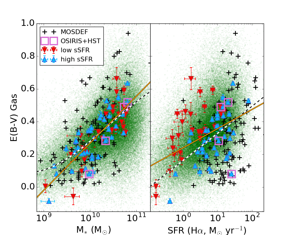
Figure 3: The relationships between $E(B-V)_{gas}$ measured from the Balmer decrement and stellar mass (left panel) and $E(B-V)_{gas}$ and SFR (H$\alpha$, right panel). DYNAMO galaxies with sSFR larger than the median sSFR for DYNAMO are plotted with blue upward triangles, and galaxies with lower sSFR’s are plotted with red downward triangles. Overplotted in each panel are the low redshift relationships between mass/SFR and $E(B-V)_{gas}$ from the SDSS (black dashed line, Garn & Best, 2010), SDSS datapoints in green (taken from the MPA-JHU VAC). Note that the apparent difference between the fit and SDSS points is a visual effect due to the density of the data points. We also plot data for high redshift galaxies taken from the MOSDEF survey taken from Reddy et al. (2015). We also plot linear fits to log₁₀($M_{*}$) and log₁₀(SFR) for DYNAMO galaxies as solid orange lines in each panel, which show DYNAMO galaxies to be in rough agreement with Garn & Best (2010). The MOSDEF sample also roughly follows the SDSS trend with $M_{*}$ (considering the large scatter found by Garn & Best, 2010) while following a steeper relation with SFR mirrored by high sSFR DYNAMO galaxies

Garn & Best (2010) find attenuation of ionized gas to correlate with both $M_{*}$ and SFR in a sample of star-forming SDSS galaxies (with AGN excluded). In Figure 3 there is an apparent offset between the fit of Garn & Best (2010) and the SDSS points, however this is simply a visual effect due to the density of plotted points. From this sample Garn & Best (2010) perform fits to the $A_{H\alpha}$ vs SFR and $A_{H\alpha}$ vs $M_{*}$ relationships independently. We compare the results for DYNAMO and MOSDEF galaxies to these local relations in Figure 3 where the results of Garn & Best (2010) are shown as black dashed lines. These relations represent polynomial fits of the form:

$$A_{H\alpha}=0.53+0.54\textrm{log}_{10}(\textrm{SFR/M}_{\odot}\textrm{ yr}^{-1})$$ (4)

$$A_{H\alpha}=0.91+0.77M^{\prime}+0.11M^{\prime 2}-0.09M^{\prime 3}$$ (5)

where $M^{\prime}$ = log₁₀($M_{*}$/10¹⁰ M_⊙).

In general, Garn & Best (2010) find that attenuation of line emitting gas increases with both SFR and $M_{*}$, as well as metallicity, in non-active, star-forming SDSS galaxies. The authors conclude that galaxy mass is the best indicator of attenuation and that, considering $M_{*}$, Equation 5 is able to predict $A_{H\alpha}$ with an error of 0.28 mag. They suggest that this is because as a galaxy increases in $M_{*}$ via star-formation it also continuously builds up a dust reservoir thus gradually increasing in $A_{H\alpha}$. More massive galaxies form greater amounts of stars during bursts and they retain a larger fraction of metals produced through star formation resulting in $A_{H\alpha}$ vs SFR and $A_{H\alpha}$ vs metallicity relationships, which are secondary to the dependence on $M_{*}$. This result is in rough agreement with a number of other similar studies (e.g. Brinchmann et al., 2004; da Cunha et al., 2010; Cortese et al., 2012b).

In Figure 3, we check for similar correlations in DYNAMO and high redshift MOSDEF data. Overplotted as a dashed line in each panel are the polynomial fits from SDSS (Garn & Best, 2010) that relates $A_{H\alpha}$ to $M_{*}$ and SFR (equations 4 and 5) where we have converted $A_{H\alpha}$ to $E(B-V)_{gas}$ assuming a Calzetti et al. (2000) attenuation curve with $R_{V}=4.0$. These fits are shown as black dashed lines. We have also plotted in green SDSS galaxies identified as star-forming, non-AGN with signal to noise cuts for H$\alpha$ and H$\beta$ of 20 and 3 respectively, which matches the requirements of Garn & Best (2010). Finally, we plot a linear fits to all DYNAMO points as orange solid lines.

Considering the left panel of Figure 3, we find a good agreement between the SDSS $M_{*}$-$E(B-V)_{gas}$ relation and the DYNAMO sample. MOSDEF galaxies roughly follow these trends as well, in agreement with the conclusion from Garn & Best (2010) that $M_{*}$ is a fundamental driver of the dust content of galaxies.

In the right panel of Figure 3, we find that correlations between $E(B-V)_{gas}$ and SFR are less clear. Considering the entire sample of DYNAMO galaxies we find a weak correlation between $E(B-V)_{gas}$ and SFR (Kendall $\tau$ = 0.31, 3.73$\sigma$ significance). In the right panel of Figure 3 we again plot a linear fit to DYNAMO points as an orange solid line, finding this to be comparable to SDSS relation of Garn & Best (2010). We note however that for both SDSS and DYNAMO galaxies there is significant scatter about the fitted relationships.

The relationship between SFR vs $E(B-V)_{gas}$ for MOSDEF galaxies appears to follow a steeper relationship compared to that of SDSS and DYNAMO. We separate DYNAMO galaxies into low and high specific SFR (sSFR=SFR/$M_{*}$) with the cut at log₁₀(sSFR)=5.35$\times$10^-10 yr^-1, the median of the DYNAMO sample. We find that at high sSFR galaxies appear to follow a similar trend between SFR and $E(B-V)_{gas}$ to that found for the MOSDEF survey while low sSFR galaxies remain uncorrelated. This may be due to an intrinsically different relationship for galaxies with very high sSFR. This may also reflect the difficulty in obtaining reliable H$\alpha$ and H$\beta$ fluxes (which are both necessary to measure $E(B-V)_{gas}$) for galaxies with a large $E(B-V)_{gas}$ and low SFR at high redshift.

We note here that Garn et al. (2010) find no evidence of an evolution in the SFR vs $E(B-V)_{gas}$ relation compared to SDSS up to $z=0.84$ considering observations of star-forming galaxies from the High Redshift Emission Line Survey (HiZELS, Geach et al., 2008). Domínguez et al. (2013) further extend this to $z\sim 1.5$ using Wide Field Camera 3 (WFC3) IR Spectroscopic Parallel (WISP) Survey data. The lack of overlap between the MOSDEF sample and low sSFR DYNAMO galaxies may result from incompleteness of the MOSDEF sample with regards to H$\beta$ detections. Garn & Best (2010) note that by including galaxies with low H$\alpha$ S/N in their sample, the median $A_{H\alpha}$ increases by 0.35 mag, which is equivalent to a change in $E(B-V)_{gas}$ of $\sim$0.1. This is comparable to the average difference between low and high sSFR DYNAMO galaxies at fixed SFR, meaning that incompleteness in the MOSDEF survey with regards to low H$\alpha$ flux galaxies may account for the lack of galaxies with low SFR and high $E(B-V)_{gas}$ in their sample.

3.2.2 $E(B-V)_{gas}$ vs $E(B-V)_{stars}$

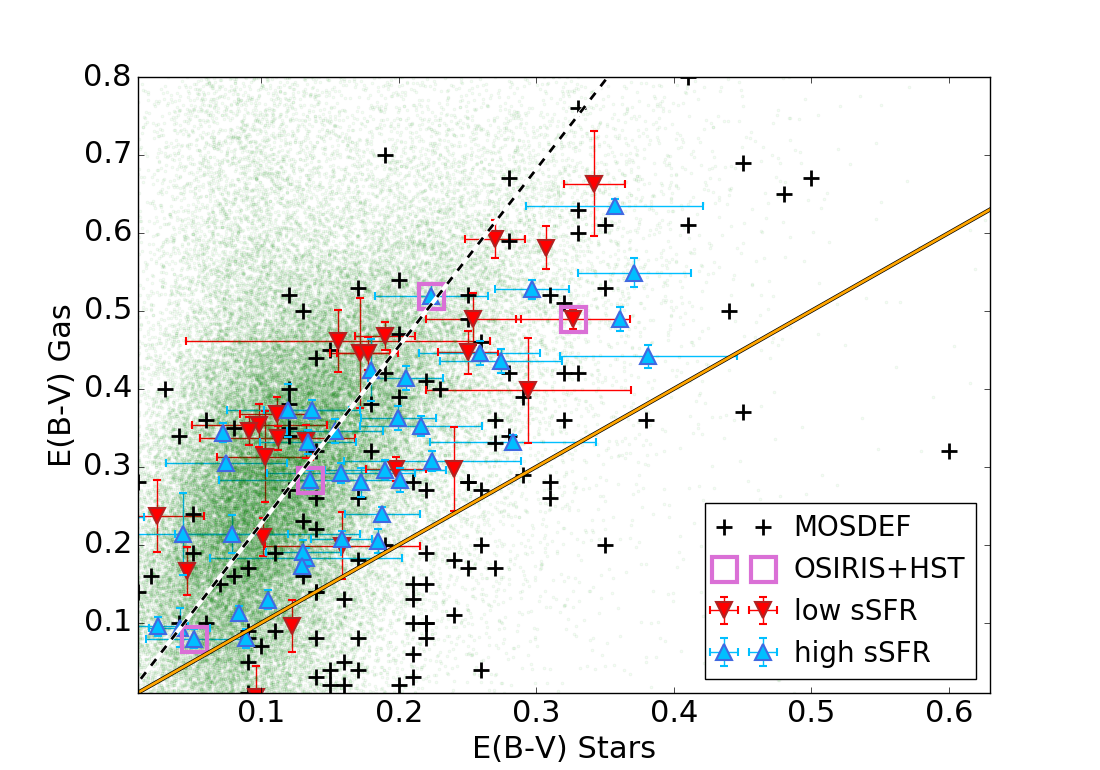
Figure 4: Here we compare integrated measures of $E(B-V)_{gas}$ from the Balmer decrement with measurements of $E(B-V)_{stars}$. Low sSFR DYNAMO galaxies are given by red downward triangles, high sSFR DYNAMO galaxies by blue upward triangles where the separation is at the median sSFR of the DYNAMO sample. High redshift MOSDEF galaxies are given by black crosses. These datapoints are plotted over the  55,000 SDSS data release 4 galaxies from the MPA-JHU VAC in green, the parent sample of the DYNAMO survey. We also indicate the local relation $E(B-V)_{stars}=0.44\times E(B-V)_{gas}$ (Calzetti, 1997) as a black dashed line, and the 1-to-1 relation using a solid line. Galaxies for which resolved attenuations are investigated are shown using purple open squares.

We also investigate the relation found for local starbursts $E(B-V)_{stars}=0.44\times E(B-V)_{gas}$ (Calzetti, 1997) for $z\sim 0.1$ galaxies with SFRs more typical of the $z>1$ universe. This relation has come under recent scrutiny, particularly at high redshifts, and its applicability to turbulent high redshift disks is unclear (Price et al., 2014; Reddy et al., 2015). In Figure 4 we plot $E(B-V)_{stars}$ versus $E(B-V)_{gas}$ for DYNAMO and MOSDEF galaxies. The solid line in this plot gives the 1-to-1 relation while the dashed line shows the local relation, $E(B-V)_{stars}=0.44\times E(B-V)_{gas}$. Again, we separate low and high sSFR DYNAMO galaxies as in Figure 3. DYNAMO and MOSDEF galaxies are plotted over the values for SDSS star-forming, non-AGN in green, taken from the MPA-JHU VAC.

We find good agreement in the relationship between $E(B-V)_{stars}$ and $E(B-V)_{gas}$ when comparing the DYNAMO and MOSDEF samples. Many galaxies from both surveys appear to be well described by the local relation, although a significant portion of both samples fall below this relation, closer to the 1-to-1 line. We perform linear fits to both datasets using the IDL routine poly_fit finding $E(B-V)_{stars}=0.78\pm 0.08\times E(B-V)_{gas}$ and $E(B-V)_{stars}=1.07\pm 0.25\times E(B-V)_{gas}$ for DYNAMO and MOSDEF galaxies, respectively. The larger scatter exhibited by MOSDEF galaxies in Figure 4 is reflected in the larger uncertainty in the fitted slope. In particular, low $E(B-V)_{stars}$ MOSDEF galaxies scatter to very low $E(B-V)_{gas}$ (below the 1-to-1 line) thus driving the correlation very close to the 1-to-1 relation. At higher $E(B-V)_{stars}$, MOSDEF and DYNAMO galaxies appear to be in better agreement.

Overall, these results suggest that applying the local relation, $E(B-V)_{stars}=0.44\times E(B-V)_{gas}$, only occasionally provides a reasonable estimate of the attenuation suffered by ionized gas emission where reliable direct estimates of $E(B-V)_{gas}$ (e.g. the Balmer decrement) are not available. In some cases, particularly for more highly attenuated galaxies, this relationship may lead to an overestimate of $E(B-V)_{gas}$, and in turn, an overestimate of SFR if this is measured from $F($H$\alpha)$. We also note that three of four galaxies making up our resolved attenuations sample fall very close to the $E(B-V)_{stars}=0.44\times E(B-V)_{gas}$ line, while one, galaxy D 13-5, falls roughly halfway between this relation and the 1-to-1 line. These differences in $E(B-V)_{stars}$ vs $E(B-V)_{gas}$ may be related to dust geometry in these galaxies, an effect that can not easily be accounted for in integrated measurements. We investigate this possibility in the remainder of this work using our combined HST and OSIRIS observations of H$\alpha$ and Pa$\alpha$.

4 Resolved Attenuation on Sub-kpc Scales

4.1 Measuring Resolved Attenuations

4.1.1 IFS Emission Line Maps

Prior to describing our method of producing IFS emission line maps, we wish to be explicit about terms. The term “spaxels” refers to the individual spectra associated with each 2D resolution element of a 3D datacube, thus distinguishing them from the “pixels” of a more traditional photometric detector.

We produce maps of emission lines from our IFS datacubes following a similar procedure to that outlined in Bassett et al. (2014). Briefly, we fit a single Gaussian profile to the emission line in question with a linear fit to the surrounding continuum included. The total flux is taken as the sum of the continuum subtracted spectrum at all positions where the fitted gaussian profile deviates from the continuum by more than 0.1%. This procedure is performed in each spaxel individually. We mask pixels in the final flux maps in which the signal to noise of a given emission line is less than one. We also mask pixels that may be associated with noise spikes (e.g. residual cosmic rays) by performing cuts on the measured velocity and velocity dispersion (also taken from our gaussian fits). Excluded are fits where velocities deviate by > 250 km s^-1 from the systemic velocity or where measured velocity dispersions less than the instrumental resolution measured from our arc exposures. Maps of Pa$\alpha$ are shown in comparison to matched HST images in Section 4.2. For galaxy G 20-2, we use the same procedure to map both [OIII] (5007 Å) and H$\beta$ allowing us to produce maps of [OIII]/H$\beta$. This is discussed in more detail in Section 4.2.

4.1.2 Matching H$\alpha$ to Pa$\alpha$ Data

A key to accurately measuring variations in attenuation in individual DYNAMO galaxies will be reliably matching the PSF of HST ($\sim$0$\aas@@fstack{\prime\prime}$1 resolution) to that of OSIRIS ($\sim$0$\aas@@fstack{\prime\prime}$6 resolution wings; $\sim$0$\aas@@fstack{\prime\prime}$15 resolution core). The overall difference in the resolution achieved between the two datasets is small due to the use of AO in our OSIRIS observations, which significantly reduces the core size of the PSF. One typical feature of AO systems, however, is that a large fraction (often a majority, $\sim$60% in our observations) of the light from a point source will be distributed in a broad wing extending significantly further than the PSF core. Because the HST PSF is more compact (and contains a larger fraction of the light in its core), measurements of the Pa$\alpha$ to H$\alpha$ ratio using OSIRIS and HST data will be artificially high in clump cores and artificially low in non-clump regions if the HST data is not matched to the AO PSF of OSIRIS.

We employ the IRAF task psfmatch to properly account for differences between the HST and OSIRIS PSFs. This task creates a convolution kernel, which can transform an input PSF to into a given output PSF through a comparison of the two in Fourier space. For our HST data, we created a PSF by averaging three stars that fall within our observed region for each galaxy, normalized to their peak flux value. Stars are selected with large angular distances from other sources to minimize contamination in the outskirts of our empirical PSF. We perform a similar procedure to create an empirical OSIRIS PSF using continuum averaged IFS observations of tip-tilt stars during a single night.

The initial PSF size of both our HST observations and the core size of the OSIRIS PSF are comparable at around $\sim$0$\aas@@fstack{\prime\prime}$15. This means our PSF matching procedure, based on Fourier transformations of our PSF images, tends to over-correct our HST photometry. Due to this, we choose to also PSF match our OSIRIS imaging to the raw PSF of HST as well using the same empirically produced PSFs described above. This second PSF matching step results in a very slight difference in our final Pa$\alpha$ image as we are matching to a slightly narrower PSF. We note that our PSF matching procedure, if done improperly could introduce trends in our maps of attenuation for our sample and furthermore the wings of the AO PSF can introduce trends even after proper matching has been performed. In Appendix A, we perform tests in order to address this, finding this not to be a large factor in our analysis.

We employ the IRAF tasks geomap and gregister to register our HST images to our OSIRIS maps. As an input, geomap requires the pixel coordinates of a number of reference positions for both images. Due to the irregular, clumpy morphologies of galaxies in our sample, we typically observe 4-5 marginally resolved star-forming regions that provide ideal reference points for this process. A caveat to this is that we assume H$\alpha$ and Pa$\alpha$ peaks to be coincident, however we consider this to be reasonable based on visual inspection of the two images. We estimate the centres of clumps from both datasets using the IRAF task ellipse and use these values to create input files for geomap. The geomap task outputs a database containing the appropriate coordinate transformations that are used as input for gregister. Together, these tasks provide a flexible tool for image matching that simultaneously handles reflection, rotation, translation, and magnification. The final results of our PSF matching and image registration are presented in Section 4.2.

4.1.3 Correcting $F($H$\alpha$) based on SPIRAL/WiFeS [NII]/H$\alpha$

We correct our HST H$\alpha$ photometry for contamination from two [NII] emission lines (at 6548 Å and 6583 Å) as these are known to fall within the spectral window of our ramp filter. To accomplish this, we investigate the contribution to our narrow band images from these lines using the original DYNAMO observations taken with the SPIRAL and WiFeS IFS. These observations are often marginally resolved spatially but can provide H$\alpha$ and [NII] fluxes and any spatial variations on 2-5 kpc scales.

In each spaxel of our SPIRAL and WiFeS datacubes we measure the ratio of the H$\alpha$ line flux to the total continuum subtracted flux in the HST ramp filter with the central wavelength matched to those of our observations of each galaxy. Here we have used the functional form for the HST ramp filter provided on the Space Telescope Science Institute website. Spaxel-to-spaxel H$\alpha$ fluxes are measured by fitting a gaussian profile giving the H$\alpha$ flux, F(H$\alpha$). We then make an estimate of the total flux of all emission lines (H$\alpha$ plus the [NII] doublet) in our narrow band filter, F(HST_NB). This is done by subtracting a linear continuum fit to the spectrum in each spaxel and summing the total flux contained in the HST ramp filter. The ratio of the fluxes measured in this way, F(H$\alpha$)/F(HST_NB), represents the multiplicative factor needed to corrected our HST H$\alpha$ photometry for the presence of [NII] in our HST ramp filter. In our three disk galaxies, D 13-5, G 04-1 and G 20-2, we find that the maps of F(H$\alpha$)/F(HST_NB) exhibit central values of 0.4-0.6 with a sudden increase to $\sim$0.9 at the large radii where H$\alpha$ uncertainties are the highest. We also note that, although there is known variation in the spectral coverage of the ACS ramp filters over the HST field of view, observed galaxies are significantly smaller than the HST field of view and, similarly, the width of the spectral features of interest are small compared to the width of the ramp filter transmission curve. For these reasons we choose to apply a flat correction for the presence of [NII] emission in our HST ramp filter based on integrated measurements of our SPIRAL datacubes.

This correction is achieved by summing the spaxels within two r-band $r_{e}$ of the galaxy centre, creating a characteristic spectrum for each galaxy. We measure F(H$\alpha$)/F(HST_NB) as described above on this summed spectrum giving the global correction value that is applied to all spaxels. The form of our correction is given as:

$$F(H\alpha)=F_{HST}\left(\frac{F(H\alpha)}{F(HST_{NB})}\right)$$ (6)

Where $F_{HST}$ is the total flux of our HST narrowband observations. This correction is applied to each pixel producing a corrected H$\alpha$ image. Our correction factors for H$\alpha$ for each galaxy are presented in Table 2. Galaxy H 10-2 has a significantly higher correction factor than the other three, and this is simply due to this galaxy having very weak $[NII]$ emission relative to H$\alpha$.

Table 2: H$\alpha$ and Pa$\alpha$ Flux Correction Factors

Galaxy	$F(H\alpha)$/$F(HST_{NB})$ correction	$c_{Pa\alpha}$ correction
	H$\alpha$, Section 4.1.3	Pa$\alpha$, Section 4.1.4
D 13-5	0.45	2.35
G 04-1	0.40	0.77
G 20-2	0.46	0.94
H 10-2	0.60	0.76

4.1.4 Correcting $F($Pa$\alpha$) Based on SDSS Balmer Decrement

As mentioned in Section 2.3.2 the spectrophotometric flux calibration of our OSIRIS datacubes suffers from a $\sim$30% systematic uncertainty due to variations in the Strehl ratio (the ratio of the maximum observed intensity to that of an ideal, diffraction limited system) of the OSIRIS PSF during a given night of observations. For this reason we choose to perform a correction to our Pa$\alpha$ maps by comparing integrated Pa$\alpha$/H$\alpha$ values based on the data presented here to H$\alpha$/H$\beta$ values measured from SDSS taken from the MPA-JHU Value Added Catalog (Tremonti et al., 2004).

For this correction, we take the integrated $E(B-V)_{gas}$ measured in Section 2.2 from the Balmer Decrement using Equation 2. We assume the value calculated in this way to be the characteristic global value of $E(B-V)_{gas}$ for a given galaxy as the emission lines in the SDSS spectra are more likely internally consistent compared with our independent observations of H$\alpha$ and Pa$\alpha$. Using this value, we can now predict the value of Pa$\alpha$/H$\alpha$ that would be detected in a region matching the SDSS fibre observation for each galaxy. This is done using Equation 2 modified in consideration of the Pa$\alpha$ and H$\alpha$ emission lines:

$$E(B-V)_{gas}=\frac{log(R_{obs}/R_{int})}{0.4[k(\lambda_{Pa\alpha})-k(\lambda_{H\alpha})]}$$ (7)

We insert the $E(B-V)_{gas}$ value calculated from the SDSS spectrum and again assume a Cardelli et al. (1989) $k(\lambda)$ and Case B recombination, which gives an intrinsic ratio of Pa$\alpha$ to H$\alpha$ of 0.123. We then solve Equation 7 for $R_{obs}$, giving the expected observed integrated ratio of Pa$\alpha$ to H$\alpha$.

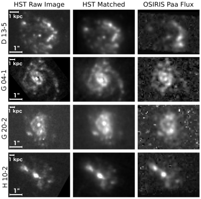
Figure 5: Our PSF matching and registration procedure applied to each of the four galaxies in our combined HST (H$\alpha$) and Keck OSIRIS (Pa$\alpha$) sample with each galaxy shown in a single row. In the left panel of each row we also include scale bars in the bottom and top left corners scale bars indicating a size of 1$\aas@@fstack{\prime\prime}$0 and 1 kpc, respectively. The colour scaling here is arbitrary as we simply wish to illustrate the results of PSF matching and image registration. There is not a large difference between the raw and matched HST photometry due to the core of the Keck AO PSF being only slightly larger than the PSF of HST. The most noticeable effects are a slight blurring due to the broad wing of the AO PSF as well as a reduction of the pixel scale to match that of OSIRIS. We note the remarkable agreement in visual morphology between the two datasets.

We next measure the integrated Pa$\alpha$/H$\alpha$ as observed for our galaxies by HST and OSIRIS in the following way. We first sum the flux of our PSF-matched HST H$\alpha$ photometry in an artificial aperture matched to that of the SDSS spectroscopic fibre. Similarly, we create an integrated spectrum of our OSIRIS data by summing all spaxels contained within an artificial SDSS aperture. The H$\alpha$ flux is calculated from the HST counts and the Pa$\alpha$ line flux is measured from our integrated spectrum as described in Section 4.1.1. This measurement of Pa$\alpha$/H$\alpha$ is thus taken in a geometric region comparable to that sampled by the SDSS fibre. In this way we can provide a correction for each galaxy by comparing our observed value with the expected $R_{obs}$ from SDSS computed above.

As H$\alpha$ fluxes from HST photometry are far more reliable than Pa$\alpha$ fluxes from our AO assisted IFS observations, we choose to correct the latter while assuming the former to be correct. The multiplicative correction factors, $c_{Pa\alpha}$, for each of our Pa$\alpha$ observations are calculated by dividing the expected value of $R_{obs}$ by the value we observe. By performing this correction we correct our Pa$\alpha$ fluxes based on a more robust measurement of the overall attenuation in our system, which will provide more reliable relative measurements (in a spatially resolved sense) as we show in Section 4.2. Values of $c_{Pa\alpha}$ are quoted in Table 2 for each galaxy.

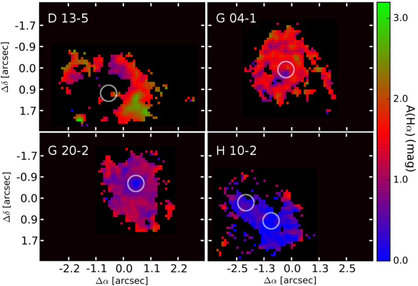
Figure 6: Maps of $A_{H\alpha}$ produced from the ratio of our Pa$\alpha$ and H$\alpha$ maps shown in Figure 5. The spread of values in individual galaxies are consistent with attenuations typical of local star-forming galaxies. Approximate locations of the continuum peaks in each galaxy are indicated with white circles. See text for detailed descriptions of individual galaxies.

Galaxies G 04-1, G 20-2, and H 10-2 have corrections between $\sim$10% and 30% while the correction for D 13-5 is significantly larger. As we show in the next Section, the distribution of dust in D 13-5 appears to be clumpier than that of the other three galaxies, and such a clumpy dust distribution may result in an intrinsically steeper attenuation law (e.g Inoue, 2005). By assuming a shallow attenuation law here, we may underestimate the difference between Pa$\alpha$ and H$\alpha$, thus overestimating the expected observed ratio Pa$\alpha$/H$\alpha$ and, in turn, $c_{Pa\alpha}$ for D 13-5. Regardless, we adopt a shallow attenuation law for consistency and again stress that, while the absolute value of $A_{H\alpha}$ may be systematically offset, the relative attenuations across the face of this galaxy are still relevant.

4.1.5 Mapping $A_{H\alpha}$

Having spatially matched our H$\alpha$ photometry to our Pa$\alpha$ IFS flux maps and applied flux corrections to both sets of observations, we can then produce resolved maps of attenuation of the four observed galaxies. First we simply produce Pa$\alpha$/H$\alpha$ maps by dividing our OSIRIS Pa$\alpha$ flux maps by our HST H$\alpha$ photometry. Next we convert the value in each pixel to $E(B-V)_{gas}$ using Equation 7, which assumes Case B recombination. Finally we convert $E(B-V)_{gas}$ to $A_{H\alpha}$ using a Cardelli et al. (1989) extinction curve and assuming $R_{V}$ = 3.1. The resulting maps of $A_{H\alpha}$ for each of our galaxies are presented in the following Section.

4.2 Results: Resolved Attenuation of Four Clumpy Galaxies

4.2.1 Maps of Attenuation From R(Pa$\alpha$, H$\alpha$)

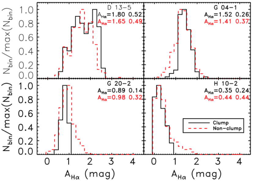
Figure 7: Histograms of $A_{H\alpha}$ in clump versus non-clump spaxels in each of our observed galaxies where clump spaxels are defined in Section 4.2.2. Within a given galaxy, the average attenuation in clumpy and non-clumpy regions are quite similar. Based on a two sample KS-test we reject the hypothesis that $A_{H\alpha}$ values come from the same parent distribution. However, this is most likely due to the fact the largest $A_{H\alpha}$ values are found in non-clump spaxels, resulting from less reliable Pa$\alpha$ flux measurements outside of bright clumps. In each panel the mean and standard deviation of clump and non-clump $A_{H\alpha}$ values are indicated with text colours matching the corresponding histograms.

PSF-matched and registered H$\alpha$ and Pa$\alpha$ maps of each galaxy are shown in Figure 5, as well as the unmatched H$\alpha$ images for reference. The matched HST and OSIRIS maps show a remarkable agreement in visual morphology suggesting an absence of patchy dust. In particular the locations and relative brightness of clumps, the term used to describe individual H$\alpha$ and Pa$\alpha$ peaks (see also, Fisher et al., 2016, for more on our definition of “clumps”), are well matched between the two datasets. This is consistent with the appearance of $A_{H\alpha}$ maps shown in Figure 6. In general, we find overall attenuation values consistent with values found for local star-forming samples or roughly 0.0 mag $\leq$ $A_{H\alpha}$ $\leq$ 3.0 mags. Within an individual galaxy variations of $A_{H\alpha}$ are typically less than 1.0 mag. This is also shown as histograms of $A_{H\alpha}$ in individual spaxels in Figure 7.

Overall we find no general correlation between the locations of clumps and increased $A_{H\alpha}$. In galaxy D 13-5 and in the central ring of G 04-1 we find variation in $A_{H\alpha}$ of $\sim$0.5-3 mag, but regions of increased attenuation do not appear coincident with any one particular clump. This could indicate a clumpy distribution of dust in these galaxies that is not spatially correlated with the locations of star-forming clumps. We also note that, due to the lower redshift of D 13-5, the OSIRIS field of view of this galaxy covers only the central star-forming region meaning a comparison of the full OSIRIS observation of D 13-5 and the central region of G 04-1 is apropos.

We find no evidence of highly attenuated regions in any of our galaxies comparable to regions seen in low redshift ULIRGS (e.g. Piqueras López et al., 2013). We also observe H$\alpha$ emission covering the entire central regions of these four galaxies strongly implying that we observe no optically thick regions such as those expected for high redshift SMGs (Blain et al., 2002). We can say with confidence that DYNAMO galaxies presented here do not contain highly attenuated clumps hosting any appreciable star-formation. Clumps such as these would be readily apparent in our OSIRIS maps of Pa$\alpha$ as well as our maps of $A_{H\alpha}$. For our small sample, clumps observed at H$\alpha$ represent the full census of highly star-forming regions. The applicability of this observation to clumpy galaxies at high redshift is still unclear, however. We now provide a more detailed description of each galaxy individually.

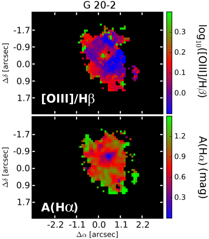
Figure 8: Comparison between the [OIII]/H$\beta$ ratio from GMOS observations and attenuation in galaxy G 20-2. This galaxy was found in integrated measurements to exhibit an excess of $E(B-V)_{stars}$ relative to $E(B-V)_{gas}$, which is generally unexpected. From the resolved observations of attenuation, the most striking feature is a drop in attenuation in the central region. Here we see that this drop corresponds to a point-like peak in [OIII]/H$\beta$ that may be indicative of a low-luminosity AGN.

D 13-5 is classified as a rotating disk from our initial SPIRAL observations, and its continuum light follows an exponential profile, suggesting that this galaxy is an undisturbed disk. H$\alpha$ photometry from HST reveals two irregularly coiled and faint spiral arms extending away from a central ring of strong star formation. The OSIRIS field of view is only slightly larger than the nuclear starburst region, and thus, it is in this region where we can reliably measure the Pa$\alpha$/H$\alpha$ ratio.

A by eye comparison between the maps of Pa$\alpha$ and H$\alpha$ flux (Figure 5) shows that the relative prominences of clumps in each map are different. This is reflected in the relatively wide variation of 0.3 < $A_{H\alpha}$ < 2.5 observed, with the largest values of $A_{H\alpha}$ $\simeq$ 2.5 found for the most Pa$\alpha$ bright clump in the bottom right corner (typical values in this area are 1.8 $\leq$ $A_{H\alpha}$ $\leq$ 2.5). This contrasts with regions surrounding the most H$\alpha$ luminous clumps where typical values are 0.8 $\leq$ $A_{H\alpha}$ $\leq$ 1.5. The amount of variation in $A_{H\alpha}$ observed in D 13-5 is the largest of any galaxy in this sample, possibly due to its lower redshift ($z\sim 0.07$) and thus higher spatial resolution.

G 04-1 was previously classified as a compact rotating disk, and subsequent observations have revealed it to host an extremely smooth exponential profile in its stellar light (Bassett et al., 2014). Line emission is arranged in clumpy spiral arms as well as an extremely luminous circumnuclear ring. The spiral arms observed in Pa$\alpha$ and H$\alpha$ are mirrored by low surface brightness spiral arms in the $K$-band continuum from our OSIRIS observations.

We see little variation (standard deviation of $A_{H\alpha}$=0.35) between the attenuation for clumps and the surrounding areas in the outer disk. Relatively large variations in the $A_{H\alpha}$ are seen in the central star-forming ring. We find an enhancement of the relative flux of Pa$\alpha$ in the top right portion of the ring as pictured in Figure 5 indicative of an increase in the column density of dust in this region where the peak $A_{H\alpha}$ in a single spaxel is measured at 2.3 mags. Similarly, there is a relative decrease of Pa$\alpha$ on the opposite side of the ring where we measure a minimum $A_{H\alpha}$ in a single spaxel of 0.5 mag. The average difference in $A_{H\alpha}$ found in spaxels between these two regions is $\sim$1 mag. This is consistent with one portion of the ring being obscured by a relatively thick dust cloud while another portion is shining through a less dusty region.

G 20-2 is an exponential disk with a number of bright clumps situated in a star-forming ring surrounding a central peak in H$\alpha$ flux (Bassett et al., 2014). We also find clumps at larger radii, the brightest of which are near the detection limits of our OSIRIS IFS observations. Overall we find a narrow range in the $A_{H\alpha}$, as seen in Figure 7, with nearly all spaxels within 0.5 magnitudes of $A_{H\alpha}$=0.9 mag. The largest values are typically associated with non-clump spaxels, however, this could be an effect of less reliable Pa$\alpha$ fluxes in these regions. Compared to typical star-forming disks locally, this galaxy can be considered to be quite average in its $A_{H\alpha}$ properties.

Overall the levels of attenuation across the entire galaxy are similar resulting in the clumpy structure being completely absent from the map of $A_{H\alpha}$. The main feature of the map of attenuation for G 20-2 is an apparent drop in the amount of attenuation in the central region, including spaxels with negative $A_{H\alpha}$ meaning that our measured line ratios are smaller than the intrinsic ratio suggested by case B recombination (implying negative attenuation). From our GMOS-IFS observations, we map [OIII]/H$\beta$, which is sensitive to the ionization state of the gas (Baldwin et al., 1981; Kauffmann et al., 2003b), in Figure 8. The extremely compact peak in [OIII]/H$\beta$ we observe could be indicative of a low-luminosity AGN. Comparing the peak value of $log_{10}([OIII]/$H$\beta)=0.38$ in the centre of G 20-2 with the average values of $log_{10}([NII]/$H$\alpha)=-0.176$ from SPIRAL observations places the centre of G 20-2 well within the AGN region of the BPT diagram (Kauffmann et al., 2003b). We note that Pa$\alpha$ to H$\alpha$ ratios less than the intrinsic ratio suggested by case B recombination have been measured for AGN by Kim et al. (2010) consistent with the values found in the central region of G 20-2.

H 10-2 has been classified as a merging system based on complex kinematics apparent in our GMOS-IFS observations. This is consistent with the OSIRIS continuum morphology as H 10-2 is the only galaxy in our sample that exhibits two peaks in continuum emission, the cores of the two merging galaxies. The bulk of the line emission is centered on these two continuum peaks, consistent with our merger hypothesis as star-formation in mergers typically results from gas funneling into the central regions (Scoville et al., 1986; Hopkins et al., 2013). Lower luminosity line emission is found in a clumpy substructure associated with the brighter (more massive) galaxy. This clumpy substructure is situated opposite the less luminous continuum peak, which may indicate that tidal forces have triggered the clumpy star formation beyond the central region (e.g. Toomre & Toomre, 1972; Sanders et al., 1986).

From the histogram of spaxel $A_{H\alpha}$ measurements it is apparent that this galaxy, consistent with the low metallicity from [NII]/H$\alpha$, has the lowest overall dust content. Similar to galaxy G 20-2, we find the lowest values in the regions with the largest continuum flux although variation from spaxel to spaxel in this region can be quite large (0.0-0.66 mag). Clumps show less variation with values falling near 0.5 mag, slightly higher than the global average. A scenario for the formation of this galaxy is an ongoing, gas-poor (and therefore low dust, Cortese et al., 2012a) merger. Although the gas fraction is relatively low (Fisher et al., 2014), the available gas can be funneled inward fueling a large SFR. Brandl et al. (2005) present IR observations of the Antennae galaxies, a famous merger, finding variation in attenuation from 0-9 magnitudes. Their false colour images reveal large, and very blue, star-forming regions consistent with intense and relatively unobscured star-formation as well as thick dust clouds. This is roughly consistent with our observations of H 10-2 assuming we are insensitive to low levels of highly obscured star-formation that may be present.

4.2.2 Clump-to-Clump Measurements of $A_{H\alpha}$

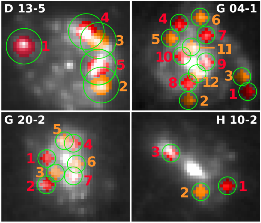
Figure 9: Apertures used to define our clump $F($Pa$\alpha)$ and $F($H$\alpha)$. In each panel we show the H$\alpha$ image of the indicated galaxy with green circles around each clump studied here. We alter the colouring of pixels in the images to red or orange to indicate exactly which pixels are selected. Red and orange colours are arbitrary and alternate in order to clearly distinguish between pixels included in clumps that are nearby one another. Clumps are numbered in order of increasing H$\alpha$ flux in order to easily identify them in Figures 10 and 11

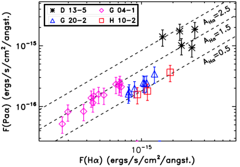
Figure 10: The relation between Pa$\alpha$ and H$\alpha$ measured in apertures centered on each clump. Results for each galaxy are plotted using different colours and symbols. Flux ratios corresponding to various constant levels of attenuation are indicated with dashed lines. Three galaxies appear to follow these trends while D 13-5 displays a larger scatter. Error bars reflect the $\sim$30% error in our OSIRIS flux calibration, most likely a systematic effect.

In this section, we compare H$\alpha$ versus Pa$\alpha$ flux for clumps in each of our galaxies. Note that in this analysis we omit central clumps as the properties of these clumps will be influenced by different physics than other clumps such as strong gas inflows associated with their being coincident with the minima of the galactic gravitational potential. For galaxies in the redshift range 0.129 < $z$ < 0.151 we measure fluxes in apertures of 0$\aas@@fstack{\prime\prime}$3, while D 13-5, which is at $z=0.07535$, we use apertures of 0$\aas@@fstack{\prime\prime}$6 to account for the roughly $2\times$ higher spatial resolution we achieve. Our apertures are illustrated in Figure 9 with clumps numbered in order of increasing H$\alpha$ flux. This analysis represents a compromise between resolving clumps and minimising the PSF effects. These apertures correspond to physical sizes of 0.86, 0.75, 0.70, and 0.79 kpc for galaxies D 13-5, G 04-1, G 20-2, and H 10-2 respectively.

We do not attempt to background subtract the flux in each aperture, which, in theory, could account for contamination from diffuse line emission. Due to the inhomogenous, clumpy nature of the emission line flux in these galaxies, a background subtraction such as this would be difficult to estimate and would likely only add to the uncertainty of our measurements.

Flux ratios measured in apertures in this way provide more robust $A_{H\alpha}$ estimates when compared to a spaxel by spaxel analysis, allowing us to clearly show if there is significant variation in attenuation from clump to clump. We first plot H$\alpha$ versus Pa$\alpha$ flux for clumps in Figure 10. For galaxies G 04-1, G 20-2 and H 10-2 we find a correlation between F(H$\alpha$) and F(Pa$\alpha$) suggesting that the attenuation suffered by different clumps in a given galaxy is quite similar (F(Pa$\alpha$)/F(H$\alpha$) = constant). We indicate with dashed lines the relation corresponding to fixed $A_{H\alpha}$ of 0.5, 1.5 and 2.5 mags.

Galaxy D 13-5 exhibits an apparent lack of correlation between F(H$\alpha$) and F(Pa$\alpha$). We believe that this not an effect of the increased spatial resolution achieved for this galaxy as we have accounted for this using a larger aperture for D 13-5. Rather, we suggest that this is an effect of larger scale variation in dust geometry, such as dust lanes, which appear in Figure 6 to obscure clumps 2 and 5 significantly more than clumps 3 and 4. We also see in Figure 10 that clumps 2 and 5 have similar attenuation, and the same is true of clumps 3 and 4, consistent with this picture. In the other three galaxies, we observe clumps that are separated by distances much larger than our PSF scale, meaning that large clump-to-clump variations like those observed in D 13-5 should be apparent in Figure 6 if present. As we noted in the previous subsection, the $A_{H\alpha}$ map of the centre of G 04-1 exhibits similar variation as that of D 13-5. Unlike D 13-5, however, the locations of the minimum and maximum are not coincident with the locations of clumps, which explains why this variation is not apparent in Figure 10.

The apparent lack of variation of $A_{H\alpha}$ measured in clumps for a given galaxy can also be seen in Figure 11 where we plot the luminosity of H$\alpha$ versus $A_{H\alpha}$ calculated as described in Section 4.1.4. Figure 10 shows that clump H$\alpha$ luminosity and attenuation are not correlated in galaxies G 04-1, G20-2, and H 10-2. We also observer a narrow spread in clump $A_{H\alpha}$ with values comparable to observations of local star-forming galaxies (Keel & White, 2001; Matthews & Wood, 2001; Takeuchi et al., 2005a; Cortese et al., 2008). Galaxy D 13-5 exhibits the widest range in clump-to-clump $A_{H\alpha}$ as shown in Figure 11. The two clumps with lower $A_{H\alpha}$ are numbers 3 and 4 in Figure 9, consistent with a visual inspection of H$\alpha$ and Pa$\alpha$ maps presented in Figure 5. G 04-1 has relatively uniform clump-to-clump $A_{H\alpha}$ with the exception of clumps 1 and 3, which are less attenuated than the others. From Figure 9 we see that these fall towards the end of the most prominent spiral arm, suggestive a low optical depth of dust at large radii. The remaining galaxies, G 20-2 and H 10-2, exhibit the smallest variation from clump to clump suggesting similar dust content across the observed regions.

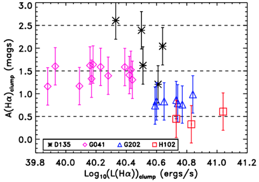
Figure 11: For each clump we plot the H$\alpha$ aperture luminosity versus the attenuation suffered at the wavelength of H$\alpha$ with symbols corresponding to each galaxy. In galaxies G 04-1, G 20-2 and H 10-2 we see little internal variation in the value of $A_{H\alpha}$, with larger differences seen when comparing average values between galaxies. In comparison, D 13-5 shows larger differences in the amount of attenuation even at fixed L(H$\alpha$), suggesting a clumpier distribution of dust. Errors on $A_{H\alpha}$ reflect the $\sim$30% error on our OSIRIS flux calibration, most likely a systematic effect.

5 Discussion

5.1 Integrated Versus Resolved Attenuation

In Section 3 we investigated the integrated properties of the full DYNAMO sample presented by Green et al. (2014). We found that highly star-forming DYNAMO galaxies are well matched to the high redshift MOSDEF sample of Reddy et al. (2015) when considering the $M_{*}$ vs $E(B-V)_{gas}$ and SFR vs $E(B-V)_{gas}$ relationships. We also compare $E(B-V)_{gas}$ vs $E(B-V)_{stars}$ for these two samples finding many galaxies to be in agreement with the relationship $E(B-V)_{stars}=0.44\times E(B-V)_{gas}$ found for local starbursts (Calzetti, 1997). At higher attenuation, however there does appear to be a trend for both DYNAMO and MOSDEF galaxies to fall below this line, closer to the relation $E(B-V)_{stars}=E(B-V)_{gas}$. Fitting a linear relationship to DYNAMO and MOSDEF data we find the relationships $E(B-V)_{stars}=0.78\pm 0.08\times E(B-V)_{gas}$ and $E(B-V)_{stars}=1.07\pm 0.25\times E(B-V)_{gas}$ respectively. Such behavior also been seen in other high redshift samples (Erb et al., 2006; Reddy et al., 2010; Kashino et al., 2013). This difference may relate to sSFR as shown by Wild et al. (2011) and Price et al. (2014), however these results are based on stacking of observations of many galaxies. Reddy et al. (2015), who select galaxies from the same parent sample as Price et al. (2014), show that there is a significant scatter in $E(B-V)_{gas}$ vs $E(B-V)_{stars}$, independent of many other galaxy properties, which may limit the usefulness of such stacking analyses.

In general, the fact that emission from ionized gas is $\sim$2 times as attenuated as the light from stars can be explained by the fact that stars migrate away from dusty star-forming regions over time while ionized gas is, by necessity, always associated with regions of intense star-formation (Charlot & Fall, 2000; Calzetti, 2001; Wild et al., 2011). Simple, screen-like geometries between stars, gas, and dust are typically assumed where stars and gas are both attenuated by a diffuse dust component while the gas is attenuated by an additional dust screen associated with star-forming regions. For galaxies G 20-2 and H 10-2 we find a relatively smooth $A_{H\alpha}$ distributions suggesting that such a simple picture may be appropriate. Galaxies G 04-1 and D 13-5, exhibits a slightly larger dispersion in $A_{H\alpha}$, which indicates that large scale variations in dust column density, i.e. a clumpy distribution of dust. The maxima and minima in attenuation for galaxy D 13-5 are spatially correlated with locations of clumps leading to a relatively large clump-to-clump variation in $A_{H\alpha}$. In contrast, maximum and minimum attenuations in G 04-1 do not correspond with clump locations, leading to little variation in clump-to-clump $A_{H\alpha}$, similar to G 20-2 and H 10-2 (see Figure 11).

Using resolved maps of attenuation we can ask: what is the difference in integrated SFR when a single $A_{H\alpha}$ is assumed versus a spatially resolved $A_{H\alpha}$ correction? To do this we measure the total attenuation corrected H$\alpha$ flux from our HST observations in two ways: first using a single integrated attenuation correction for H$\alpha$, taken from the MPA-JHU VAC values, and second by correcting individual pixels based on our $A_{H\alpha}$ maps. For galaxies D 13-5, G 04-1, G 20-2, and H 10-2 we measure fractional differences, $F($H$\alpha_{int})-F($H$\alpha_{map})$/$F($H$\alpha_{int})$, of +0.28, -0.05, +0.03, and +0.12 respectively. Thus we find using an integrated attenuation corrections that the SFR in these four galaxies ranges from a 5% under prediction to a 28% over prediction of the SFR compared to resolved attenuation corrections, with no systematic trend between galaxies.

The largest difference between these two SFR estimates is found for our lower redshift galaxy, D 13-5. This galaxy also exhibits a large variation in $A_{H\alpha}$ from clump to clump, which we attribute to large scale dust features. Clumps in galaxies G 20-2 and H 10-2 have large enough separations that we should resolve similar differences in attenuation if they are present. In G 04-1 we observe a similar variation in our $A_{H\alpha}$ map, however maximum and minimum attenuations do not correlate with clumps meaning assuming a flat $A_{H\alpha}$ correction will have less of an effect on the integrated SFR. This may also account for the fact that in integrated measurements galaxies G 04-1, G 20-2, and H 10-2 fall on the $E(B-V)_{stars}=0.44\times E(B-V)_{gas}$ relation while D 13-5 sits significantly below this, as an assumption of a simple screen dust geometry is implicit in these calculations. This assumption may not be appropriate for a clumpy distribution of dust that attenuates different star-forming regions at different levels, which may be more representative of D 13-5. Of course, from a sample of four galaxies it is not possible to extrapolate to the full sample of clumpy high redshift galaxies, again highlighting the necessity of larger samples of resolved attenuation observations. The observation that SFRs in DYNAMO galaxies may be biased and overpredicted could have important implications regarding the normalisation of the main sequence of star-forming galaxies at high redshift.

5.2 An Absence of Highly Attenuated Clumps

The main advantage of using IR emission lines for studying attenuation in galaxies is the low intrinsic attenuation at these wavelengths allowing lines such as Pa$\alpha$ to emerge from deep within dust-enshrouded regions. This means that using observations of Pa$\alpha$ will be significantly more sensitive to regions of high dust obscuration than optical and UV techniques such as the Balmer decrement or the UV slope, $\beta$ (Meurer et al., 1999). For foreground dust geometries the implication is that optical techniques will be biased towards unextincted regions and may not be sensitive to star formation located behind highly obscuring dust clouds (Calzetti, 1997).

One key result from our HST+OSIRIS sample, which is apparent from Figure 5, is a lack of extremely bright clumps in our Pa$\alpha$ maps that are absent (or at least very low luminosity) in our H$\alpha$ imaging. This would be indicative of star formation that is sitting behind a very high column density region of dust, which completely attenuates the optical emission but allows the IR emission to shine through. Genzel et al. (2013) have performed semi-resolved observations of CO (3-2) in a single main-sequence galaxy at $z=1.53$ from the PHIBSS survey (Tacconi et al., 2010, 2013), finding evidence of large quantities of molecular gas spatially correlated with their map of $A_{V}$ (from SED fitting). From this observation they estimate that, assuming the dust is situated in a single foreground cloud, $A_{V}$ in these regions could reach as high as $\sim$50 mag. Assuming a Cardelli et al. (1989) dust curve this implies an attenuation of $\sim 8$ mag even at the wavelength of Pa$\alpha$. We estimate that an individual star-forming clump situated behind such a cloud would require a SFR $\sim$50 $M_{\odot}$ yr^-1 to be detected by our OSIRIS observations of our most nearby galaxy, thus we can not rule out the possibility of lower levels of highly obscured star-formation in DYNAMO galaxies. In local star-forming galaxies, however, dust is most likely clumped on sub-kpc scales and/or mixed with stars and gas (e.g. Bedregal et al., 2009; Liu et al., 2013; Piqueras López et al., 2013; Boquien et al., 2015). Thus highly star-forming (and therefore large, Wisnioski et al., 2012) clumps are unlikely to be fully obscured by high column density dust clouds. Furthermore, we observe a maximum H$\alpha$ attenuation of $\sim$3 mag thus a jump from this to regions of $A_{H\alpha}$ > 10 with no intermediate cases is unlikely. For these reasons we suggest that the levels of highly attenuated star-formation in clumpy DYNAMO galaxies are minor relative to that currently observable in clumps.

These result may carry implications regarding observations of clumpy main-sequence galaxies at high redshift (Wright et al., 2009; Förster-Schreiber et al., 2009; Wisnioski et al., 2011; Epinat et al., 2012; Swinbank et al., 2012; Wisnioski et al., 2015). Resolving clumps in $z\sim 1-2$ star-forming galaxies in the IR, as is done here for DYNAMO galaxies at $z\sim 0.1$, is not possible using current facilities. If the physical conditions of DYNAMO galaxies can be considered as similar to the conditions in clumpy high-$z$ disks, then it should be reasonable to assume that observations of H$\alpha$ can, in some cases, provide a full census of star-forming regions in a given galaxy. We stress again, though, that this result is based on observations of four galaxies, thus, it is not reasonable to extrapolate to large samples of star-forming galaxies at high-redshift. Future observations probing the IR regime of high redshift galaxies such as those performed using the James Webb Space Telescope will further shed light on these issues.

5.3 Spatial Variation in Attenuation

Table 3: Average Clump and Non-Clump Attenuation Values

ID	<$A_{H\alpha}($clump$)$>	<$A_{H\alpha}($non-clump$)$>	$A_{H\alpha,int}$
	mag	mag	mag
D 13-5	1.80$\pm$0.52	1.65$\pm$0.49	1.46
G 04-1	1.52$\pm$0.26	1.41$\pm$0.37	1.55
G 20-2	0.89$\pm$0.14	0.98$\pm$0.32	0.86
H 10-2	0.35$\pm$0.24	0.44$\pm$0.44	0.21

We observe a range of attenuation values both between galaxies as well as within individual galaxies with typical values 0.0 < A_Hα < 3.0 (see Figure 7). This result is generally consistent with attenuation measurements of star bursting galaxies at both low (Calzetti et al., 2000) and high redshifts (Förster Schreiber et al., 2011). This result is also consistent with the IFS observations of Boquien et al. (2009) who find A_V values of $0.1-1$ for a sample of low SFR, face-on disks. Highly attenuated LIRGS and ULIRGS on the other hand, are found to have typical median A_V values of 4-6 mag with individual measurements ranging from $\sim$1 to $\sim$20 mags within a single galaxy (Bedregal et al., 2009; Piqueras López et al., 2013). The general result is that dust is geometrically clumpy, and galaxies with larger overall dust content host the highest column density clumps. Confirming this observation however will rely upon measurements of attenuation in larger samples of galaxies of various types with sub-kpc resolution.

The fact that we observe a large spread in values for galaxy D 13-5 may be related to the lower redshift of this object when compared with the remainder of the sample. This redshift distance corresponds to an increased spatial resolution for this object of 863 pc when compared to $\sim$1.5 pc at high redshift. This is consistent with the study of Boquien et al. (2015) who test the effects of resolution on the resolved attenuation measurements of M33. The general result of this study is that spatial variation in attenuation maps becomes more apparent for small spatial sampling scales, with differences reducing to $\sim 0$ at scales of $\sim$1 kpc. We perform a simple test by rebinning the $A_{H\alpha}$ map of D 13-5 by a factor of two and find the same spread of values as in the unbinned image. The significant enhancement in $A_{H\alpha}$ at the bottom right of D 13-5 relative to the rest of the galaxy is still apparent, suggesting differences in attenuation seen in Figure 6 is due to large scale variation in dust covering fraction (e.g. a dust lane). We have also pointed out that the OSIRIS observations of D 13-5 cover only the central star-forming ring that can be considered comparable to the central region of G 04-1 observed at a higher spatial resolution. In the star-forming ring of G 04-1 we observe a similarly large variation in attenuation giving further evidence that the observed variation in attenuation is not an effect of resolution. In G 04-1, this variation does not correlate with clumps, thus clump-to-clump measurements, and likely integrated measurements, of SFR are less affected by variable attenuation in G 04-1 when compared with D 13-5.

The spatial resolutions probed in this study are roughly comparable to the measured size of clumps in these galaxies. This means that while resolving dust substructure within individual clumps is not possible, differences in attenuation from clump to clump should be apparent if present. It is therefor remarkable that in each galaxy there is such a small variation in attenuation from clump to clump as shown by Figures 10 and 11. In particular, galaxies G 04-1, G 20-2, and H 10-2 each exhibit a very flat relationship between clump H$\alpha$ luminsoity and $A_{H\alpha}$. This may be due to the turbulent nature of these galaxies that can result in significant mixing of stars, gas, and dust. A similar result is found by Kreckel et al. (2013) for galaxy NGC 2146, the strongest starburst system in their sample. We note, however, that comparing clump and non-clump spaxels in our DYNAMO galaxies using a two sample KS-test rejects the hypothesis that $A_{H\alpha}$ values are taken from the same parent distribution. This is most likely due to the fact the largest $A_{H\alpha}$ values are found in non-clump spaxels, resulting from less reliable Pa$\alpha$ flux measurements outside of bright clumps. Figure 7 shows that the average values of $A_{H\alpha}$ between clump and non-clump regions are very similar.

A flat distribution of $A_{H\alpha}$ in turbulent DYNAMO galaxies is consistent with models of the evolution of clumpy star formation such as those of Bournaud et al. (2014) who argue for long-lived clumps that experience both strong inflows and outflows. Such activity will greatly facilitate the mixing of material between clumps and between clumpy and non-clumpy regions. Such a model naturally results in relatively flat spatial distributions in $A_{H\alpha}$. We do find significant variation in the average attenuation of clumps from galaxy to galaxy, however this is likely due to differences in stellar mass. This is consistent with our investigation of integrated attenuations as we find the four galaxies in our resolved attenuations sample to follow a trend of increasing $E(B-V)_{gas}$ with increasing mass in Figure 3.

6 Conclusions

In this paper, we have presented integrated attenuation measurements of a sample of 67 DYNAMO galaxies from SDSS observations as well as a resolved study of attenuation in four highly star-forming DYNAMO galaxies. The latter is achieved by combining high-resolution H$\alpha$ imaging from HST with AO-assisted IFS from OSIRIS at Keck targeting the Pa$\alpha$ emission line in the IR. By utilising emission at long wavelengths we are sensitive to highly attenuated star-formation which may be missed by observations of optical emission lines. The conclusions of our analyses are as follows:

• From integrated observations we find that DYNAMO galaxies exhibit a larger spread in integrated SFR at fixed $E(B-V)_{gas}$ than the high redshift MOSDEF sample (Reddy et al., 2015), however, considering only highly star forming DYNAMO galaxies alone there is much better agreement.

• Comparing integrated $E(B-V)_{gas}$ and $E(B-V)_{stars}$ for DYNAMO and MOSDEF we find a similar trend that, at high attenuation, galaxies deviate from the local starburst relation $E(B-V)_{stars}=0.44\times E(B-V)_{gas}$ moving towards $E(B-V)_{stars}=E(B-V)_{gas}$. We fit linear relationships to DYNAMO and MOSDEF galaxies finding $E(B-V)_{stars}=0.78\pm 0.08\times E(B-V)_{gas}$ and $E(B-V)_{stars}=1.07\pm 0.25\times E(B-V)_{gas}$ respectively. For DYNAMO galaxies this does not seem to depend on SFR, however.

• In four DYNAMO galaxies we find no evidence for highly attenuated and strongly star-forming clumps, which would be readily apparent in our Pa$\alpha$ observations. This does not preclude the possibility of lower levels of highly obscured star-formation, however, such star-formation would likely be negligible when compared to the extreme SFRs of observed clumps.

• We find mild spatial variation in the amount of attenuation depending on the spatial location within a given galaxy. Values of $A_{V}$ vary from $\sim 0$ to $\sim 3$ with most values in the 0.5-1.5 range, typical of local star-forming galaxies. Within a single galaxy, the spread in values is $\sim$1 mag.

The latter two conclusions, from our resolved observations, suggest that the bulk of the star-formation present in these galaxies is already accounted for in our H$\alpha$ imaging even though it will be more affected by the presence of dust. We stress, however, that this result is based on observations of four galaxies and they may not be immediately applicable to the general population of clumpy, star-forming galaxies at $z>1.5$. In future work we plan on investigating the integrated attenuations of DYNAMO galaxies by comparing $E(B-V)_{gas}$, from the Balmer decrement, and $E(B-V)_{stars}$, computed through full SED fitting including far-IR data constraining dust emission. Work investigating the direct detection of emission from dust in DYNAMO galaxies is currently underway using observations from the Wide-field IR Survey Explorer (WISE, Wright et al., 2010) that will compare dust masses with molecular gas masses (from CO detections using PdBI, Fisher et al., 2014, White et al. in prep). These analyses will help us to test the applicability of local calibrations (e.g. Calzetti, 1997) to star-forming galaxies at high redshift and how the relative attenuations suffered by stars and gas relate to other galaxy properties.

The authors would like to thank Naveen Reddy for providing data from the MOSDEF project for comparison to our observations as well as Katinka Geréb for constructive comments in the preparation of this manuscript. We would also like to thank the anonymous referee for helping to improve the readability of this work. Support for this project is provided in part by the Victorian Department of State Development, Business and Innovation through the Victorian International Research Scholarship (VIRS). This research was supported under Australian Research Council’s Discovery Projects funding scheme (project number DP130101460). (Some of) The data presented herein were obtained at the W.M. Keck Observatory, which is operated as a scientific partnership among the California Institute of Technology, the University of California and the National Aeronautics and Space Administration. The Observatory was made possible by the generous financial support of the W.M. Keck Foundation. The authors wish to recognize and acknowledge the very significant cultural role and reverence that the summit of Mauna Kea has always had within the indigenous Hawaiian community. We are most fortunate to have the opportunity to conduct observations from this mountain. Portions of this work are based on observations obtained at Gemini Observatory (GS-2011B-Q-88, processed using the Gemini IRAF package), which is operated by the Association of Universities for Research in Astronomy, Inc., under a cooperative agreement with the NSF on behalf of the Gemini partnership: the National Science Foundation (United States), the National Research Council (Canada), CONICYT (Chile), Ministerio de Ciencia, Tecnología e Innovación Productiva (Argentina), and Ministério da Ciência, Tecnologia e Inovação (Brazil). This research has made use of data from HRS project. HRS is a Herschel Key Programme utilising Guaranteed Time from the SPIRE instrument team, ESAC scientists and a mission scientist. The HRS data was accessed through the Herschel Database in Marseille (HeDaM - http://hedam.lam.fr) operated by CeSAM and hosted by the Laboratoire d’Astrophysique de Marseille.

Appendix A Testing the Effects of PSF Matching

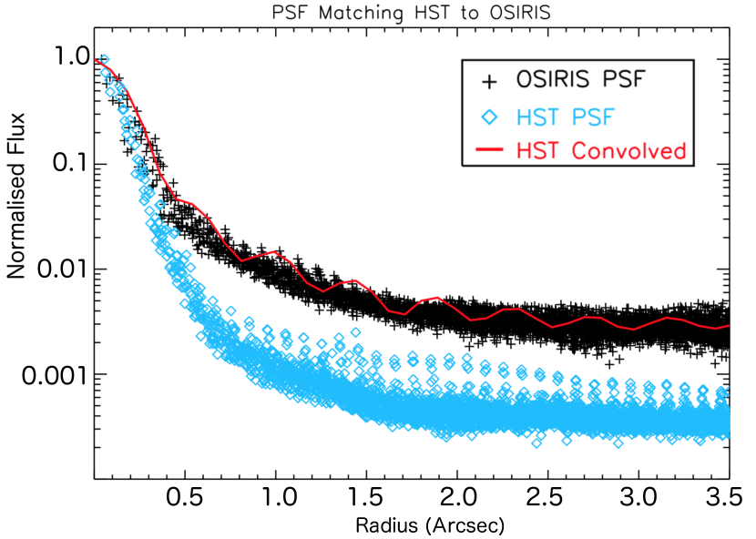
Figure 12: The results of our PSF matching procedure. We plot the input data for our empirical OSIRIS (black crosses) and HST (blue diamonds) PSFs normalized to their respective central fluxes. Each PSF was constructed from observed stars during our program as described in Section 4.1.2. Overplotted in red is the binned radial profile of our output HST PSF after being matched to OSIRIS using the IRAF task psfmatch. The oscillations apparent in the convolved profile are a result of Fourier Transforms used by psfmatch in combination with the small field of view of OSIRIS.

We would like to understand any possible biases that may be introduced into our observed maps of $A_{H\alpha}$ as a result of our PSF matching procedure. We illustrate the difference between the HST and OSIRIS PSFs, as well as the result of applying our PSF matching procedure directly to our HST PSF, in Figure 12. The PSF effects here may be quite complex due to the bright PSF wings and rapid temporal variation. Furthermore, these effects will depend on the relative proximity of bright clumps as well as the relative brightness of clump versus disk light. To test these effects we create two additional maps of $A_{H\alpha}$ for each galaxies and compare these to the maps presented in Section 4.2.1. Together, these make up our three test cases described below:

Fiducial Map: As a starting point for this test we take the maps presented in Section 4.2.1. To be explicit here, these maps are produced by performing the IRAF task psfmatch using empirical PSFs for our HST and OSIRIS observations and registering the images as described in the text. We divide our OSIRIS Pa$\alpha$ map by our PSF matched HST H$\alpha$ map and convert this to $A_{H\alpha}$ using Equation 7. As this is the method used in our analysis, we will refer to this as the fiducial case.

PSF Only: In this instance we would like to isolate the effects of our PSF matching procedure. This is done by producing an artificial Pa$\alpha$ map from our H$\alpha$ observations. To achieve this we perform the PSF matching procedure described in the text on our HST H$\alpha$ image, then scale it by a factor determined from Equation 7 to give a value of $A_{H\alpha}$ of 1 mag. We then divide this artificial Pa$\alpha$ map by the original (non-PSF matched) HST H$\alpha$ map and convert to $A_{H\alpha}$ using Equation 7. Had we not performed a PSF matching step, this would return a flat $A_{H\alpha}$ map with a value of 1 (by design), thus any variation in the produced map will be entirely due to our PSF matching procedure.

Unmatched: Finally we create a map of $A_{H\alpha}$ applying no PSF matching to either map whatsoever. We simply register our unmatched HST H$\alpha$ map to our OSIRIS Pa$\alpha$ map without PSF matching, divide this by our Pa$\alpha$ map, and convert to $A_{H\alpha}$ using Equation 7. By comparing this case with the fiducial map described above we can isolate the effect our PSF matching has on the maps presented in Section 4.2.1.

Maps of Pa$\alpha$ to H$\alpha$ for these three cases for galaxy G 20-2 are shown in Figure 13 alongside the HST map of H$\alpha$ without PSF matching. The intrinsic value for this ratio assuming Case B recombination is 0.123. Regions with Pa$\alpha$/H$\alpha$ greater than indicate areas of nonzero $A_{H\alpha}$. The key difference between the fiducial case and the two test cases is the presence of clumpy substructure with the test cases showing a correspondence between clump loci and minima in $A_{H\alpha}$. This is due to the lower Strehl ratio of the OSIRIS PSF, with a large fraction of the light of each spaxel being blurred to larger radii, resulting in an artificially low Pa$\alpha$ to H$\alpha$ ratio. The fact that both test cases exhibit this behavior gives us confidence that this is a direct result of the difference in PSF shape between OSIRIS and HST.

We plot the comparison between the three $A_{H\alpha}$ maps described above in Figure 14. In each panel we plot the normalised quantity, $A_{H\alpha}$/median($A_{H\alpha}$) as a function of $F($Pa$\alpha)$/mean($F($Pa$\alpha)$). Values for the fiducial $A_{H\alpha}$ are given by black points with large black circles indicating binned values (with bin sizes of 0.2 in $F($Pa$\alpha)$/$<F($Pa$\alpha)>$). Red points give the PSF Only values with open red diamonds indicating the binned values. Finally, the thick blue line in each panel indicates the binned values for the unmatched case.

We find that for both the PSF Only and Unmatched cases $A_{H\alpha}$ decreases steadily with increasing Pa$\alpha$ flux. This is in contrast to the roughly flat, or rising in the case of D 13-5 and H 10-2, behavior of our Fiducial case. This difference is entirely do to the difference between the HST and OSIRIS PSF. The latter includes a broad component, which is a common feature of AO observations, thus distributing light from bright pixels into lower flux regions. In the two cases with poorly matched PSFs (PSF Only and Unmatched) this induces an artificial dearth of Pa$\alpha$ flux in high flux regions, and, therefore, and under prediction of $A_{H\alpha}$. The fact that our true unmatched images are well matched in behavior by the simulated case using only the HST images (PSF Only) give us added confidence that our OSIRIS PSF is a reasonable representation of the response of our AO system to a point source. We note that Figure 14 shows a much larger spread for spaxels with low Pa$\alpha$ flux and in the lowest flux bins all three test cases seem to disagree. While this could be due to more intrinsic variation in line-of-sight attenuation at low Pa$\alpha$ flux, more likely it reflects spaxels that are near the detection limit as well as the contamination of low flux spaxels by clump light blurred by the wings of the AO-PSF. For this reason we stress some caution in over interpretation of $A_{H\alpha}$ in low flux regions. The large spread for individual spaxels also suggests that individual spaxel measurements of $A_{H\alpha}$ are not entirely trustworthy, thus the value of maps presented in Figure 6 is in the average behavior of $A_{H\alpha}$ in different spatial regions of the observed galaxies. This will trace large scale (i.e. clump-to-clump) variations in attenuation that can be indicative of regions of very high dust column density such as dust lanes.

We next test how this will affect integrated (aperture) measurements of $E(B-V)$ for individual clumps in each galaxy. For clump measurements we sum pixels/spaxels in apertures centered on each clump and compute the ratio of Pa$\alpha$ to H$\alpha$ in these apertures. For each clump we measure this ratio in apertures of increasing size for our fiducial measurement as well as the two test cases described above. We then compute a value of $E(B-V)$ assuming a Cardelli et al. (1989) attenuation curve. We normalize the $E(B-V)$ profiles produced in this way by the value measured in large apertures in order to compare results from clump to clump. The results of this test are plotted in Figure 15 with a panel for each galaxy. Profiles presented in this Figure represent the average clump profile in a given galaxy. The black solid line gives our fiducial measurements while red and green lines give our PSF Only and Unmatched match test cases respectively. In each panel the profiles are normalised to the value measured for very large apertures that effectively encompass the entire galaxy. Values in these large apertures will be negligibly altered by any PSF effects as in all three cases all of the observed emission from clumpy and non-clumpy regions will be included.

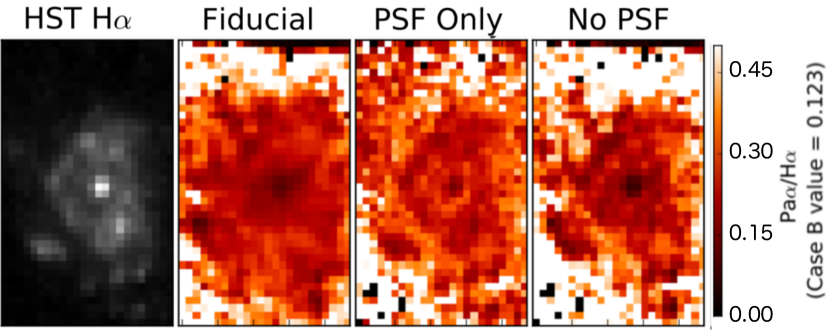
Figure 13: Maps of Pa$\alpha$/H$\alpha$ for galaxy G 20-2 showing the three test cases described in Appendix A as well as the HST map of H$\alpha$ (without PSF matching). From left to right this shows the H$\alpha$ map, our fiducial case, PSF matching only, and no PSF matching. The intrinsic value of this ratio assuming Case B recombination is 0.123, thus larger values indicate regions where $A_{H\alpha}$ > 0. The two test cases show a correspondence between H$\alpha$ peaks (clumps) and minima in $A_{H\alpha}$, while clumpy substructure is not apparent in our fiducial case. Our two test cases appear qualitatively similar, suggesting that the apparent substructure is an artificial effect induced by difference in the PSF.

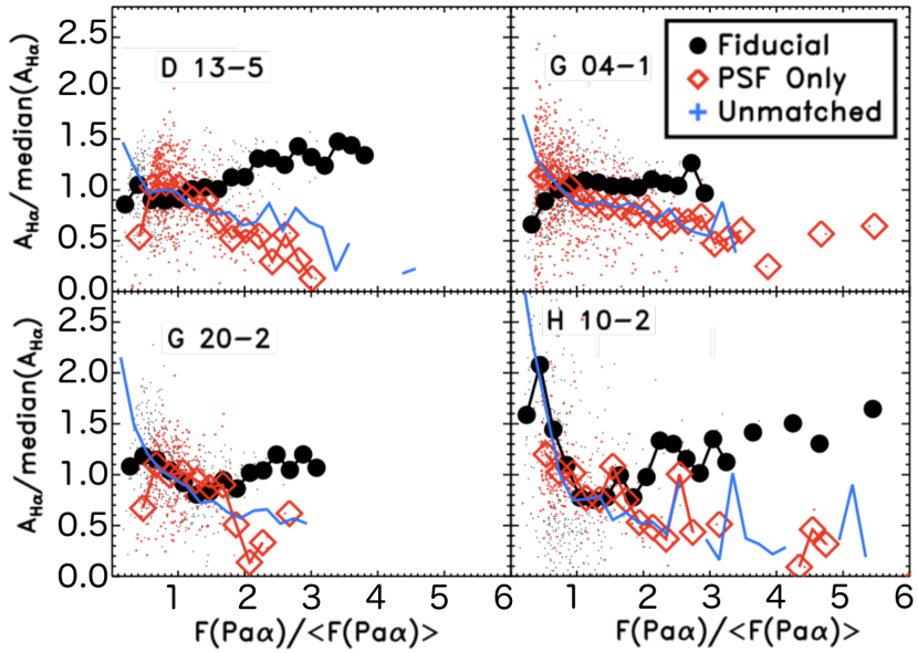
Figure 14: For each galaxy we compare $A_{H\alpha}$/median($A_{H\alpha}$) as a function of the Pa$\alpha$ flux in a given pixel normalized by the average flux for that galaxy. The small black points give individual spaxel measurements for our observations and the large black circles are binned values. Similarly we create mock observations described in Section A using our PSF matched and non-matched HST images, these values are plotted as red points for spaxels and red diamonds for binned (bin sizes of 0.2 in $F($Pa$\alpha)$/$<F($Pa$\alpha)>$) values. Finally we plot as a solid blue line the results using the observed Pa$\alpha$ and H$\alpha$ maps without PSF matching. This non-PSF matched case is well matched to the PSF only test case, thus our PSF matching procedure appears to accurately capture the true difference in our observed PSFs.

For both of our test cases we find a rising profile of $E(B-V)$ with aperture size. This is expected considering the AO PSF, which will redistribute Pa$\alpha$ flux from the centre of a given clump to larger radii, and in agreement with maps of Pa$\alpha$/H$\alpha$ shown in Figure 13. HST photometry of H$\alpha$ does not suffer from this effect and clumps observed at H$\alpha$ will be more centrally concentrated. For our fiducial case, for which PSF matching has been performed, we find that $E(B-V)$ decreases with aperture radius in all cases. We conclude that, because our unmatched and PSF only test cases seem to typically exhibit similar behavior, our PSF matching procedure provides a reasonable match between our two datasets. We also find that $r=0\aas@@fstack{\prime\prime}3$ apertures are satisfactory and adopt these for measuring $A_{V}$ in DYNAMO clumps in Section 4.2.2. This is not unreasonable as apertures of this size are comparable to the core size of the OSIRIS AO PSF, thus encompassing a majority of the well resolved portion of the clump light.

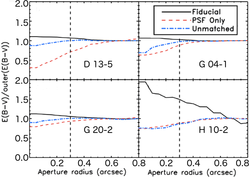
Figure 15: For each galaxy we measure $E(B-V)_{gas}$ in apertures of increasing radii for our PSF matched data, as well as the two test cases described in Section A, both of which do not include PSF matching. Here we plot $E(B-V)_{gas}$ as a function of aperture size averaged over all of the clumps within a given galaxy. Individual profiles are found to be less regular due variation induced by noise. We normalize each profile by the value in the largest apertures prior to averaging to account for absolute differences between each clump. For all galaxies we find the test cases exhibit a rising profile, a signature of the PSF mismatch, while our observations show a decrease. In each panel we plot a vertical dashed line at 0$\aas@@fstack{\prime\prime}$3, which roughly marks the transition at which the test case using both HST and OSIRIS data comes intro agreement with our observations. We note that this is typically quite close ($\sim$5%) from the value in large apertures, reflecting the limitations imposed by the broad wings of the AO PSF.

Appendix B GMOS Image Registration

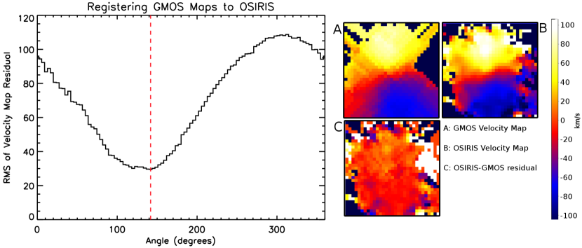
Figure 16: left: diagnostic plot of our GMOS registration procedure. Briefly we clip each image and match the galaxy centre based on the continuum image. The standard deviation of the values in the velocity map residual (OSIRIS_vm-GMOS_vm) is measured for all angles and the necessary rotation is taken as the minimum of the distribution, marked with a red dashed line. right: examples of clipped images used to produce the left plot. Panel A shows the GMOS velocity map rotated by the angle indicated by the red dashed line, panel B shows the OSIRIS velocity map, and panel C shows the residual velocity map. All three maps are shown using the same colour scaling.

We register maps produced from our GMOS IFS observations (see Bassett et al., 2014) to those from OSIRIS based on the kinematic maps produced from the two datasets. Due to the lower spatial resolution of the GMOS observations the clumps begin to blend together hampering our ability to use the registration method described for HST. In this case we wish to match maps from two IFS datasets, both of which can provide a wealth of spatially resolved information. We perform our registration in two steps, the first of which is to match the centroid position of the continuum image of the galaxy for both instruments. We then shift the velocity and velocity dispersion maps produced from our GMOS observations based on this shift and produce rotated versions of these kinematic at a large number of rotation angles locating the angle that minimizes the difference average residual in both velocity ($v_{OSIRIS}-v_{GMOS,rotated}$) and velocity dispersion ($\sigma_{OSIRIS}-\sigma_{GMOS,rotated}$). We also perform the test adjusting the x and y shifts estimated based on the continuum images by $\pm$0$\aas@@fstack{\prime\prime}$3 to account for the seeing of our GMOS observations. An example of this procedure is shown in Figure 16.

After selecting the best fitting shift and rotation angle, these are applied to the maps of [OIII]/H$\beta$, giving a more complete understanding of the state of the gas in DYNAMO HST+OSIRIS galaxies. In particular, variations in [OIII]/H$\beta$ may indicate the presence of ionizing processes other than star-formation that may be responsible for a portion of the ionizing radiation. In this case, Hydrogen line ratios which we use to estimate the amount of attenuation suffered by ionized gas, may no longer follow the relation given by Case B recombination resulting in a poor estimate of $A_{V}$. Registered maps of [OIII]/H$\beta$ from GMOS to our HST+OSIRIS maps of nebular attenuation in Figure 8 in Section 4.2.

References

- Alonso-Herrero et al. (2006) Alonso-Herrero A., Rieke G. H., Rieke M. J., Colina L., Pérez-González P. G., Ryder S. D., 2006, ApJ, 650, 835
- Baldwin et al. (1981) Baldwin J. A., Phillips M. M., Terlevich R., 1981, PASP, 93, 5
- Bassett et al. (2014) Bassett R., et al., 2014, MNRAS, 442, 3206
- Battisti et al. (2016) Battisti A. J., Calzetti D., Chary R.-R., 2016, ApJ, 818, 13
- Bedregal et al. (2009) Bedregal A. G., Colina L., Alonso-Herrero A., Arribas S., 2009, ApJ, 698, 1852
- Berman (1936) Berman L., 1936, MNRAS, 96, 890
- Blain et al. (2002) Blain A. W., Smail I., Ivison R. J., Kneib J.-P., Frayer D. T., 2002, Phys. Rep., 369, 111
- Boquien et al. (2009) Boquien M., et al., 2009, ApJ, 706, 553
- Boquien et al. (2015) Boquien M., et al., 2015, A&A, 578, A8
- Boselli et al. (2010) Boselli A., et al., 2010, PASP, 122, 261
- Boselli et al. (2015) Boselli A., Fossati M., Gavazzi G., Ciesla L., Buat V., Boissier S., Hughes T. M., 2015, A&A, 579, A102
- Bournaud et al. (2014) Bournaud F., et al., 2014, ApJ, 780, 57
- Brandl et al. (2005) Brandl B. R., et al., 2005, ApJ, 635, 280
- Brinchmann et al. (2004) Brinchmann J., Charlot S., Heckman T. M., Kauffmann G., Tremonti C., White S. D. M., 2004, arXiv:astro-ph/0406220,
- Bruzual & Charlot (2003) Bruzual G., Charlot S., 2003, MNRAS, 344, 1000
- Calzetti (1997) Calzetti D., 1997, in Waller W. H., ed., American Institute of Physics Conference Series Vol. 408, American Institute of Physics Conference Series. pp 403–412 (arXiv:astro-ph/9706121), doi:10.1063/1.53764
- Calzetti (2001) Calzetti D., 2001, PASP, 113, 1449
- Calzetti et al. (1997) Calzetti D., Meurer G. R., Bohlin R. C., Garnett D. R., Kinney A. L., Leitherer C., Storchi-Bergmann T., 1997, AJ, 114, 1834
- Calzetti et al. (2000) Calzetti D., Armus L., Bohlin R. C., Kinney A. L., Koornneef J., Storchi-Bergmann T., 2000, ApJ, 533, 682
- Calzetti et al. (2005) Calzetti D., et al., 2005, ApJ, 633, 871
- Cambrésy et al. (2011) Cambrésy L., Rho J., Marshall D. J., Reach W. T., 2011, A&A, 527, A141
- Cardelli et al. (1989) Cardelli J. A., Clayton G. C., Mathis J. S., 1989, ApJ, 345, 245
- Chabrier (2003) Chabrier G., 2003, PASP, 115, 763
- Charlot & Fall (2000) Charlot S., Fall S. M., 2000, ApJ, 539, 718
- Cortese et al. (2008) Cortese L., Boselli A., Franzetti P., Decarli R., Gavazzi G., Boissier S., Buat V., 2008, MNRAS, 386, 1157
- Cortese et al. (2012a) Cortese L., et al., 2012a, A&A, 540, A52
- Cortese et al. (2012b) Cortese L., et al., 2012b, A&A, 544, A101
- Cucciati et al. (2012) Cucciati O., et al., 2012, A&A, 539, A31
- Davies (2007) Davies R. I., 2007, MNRAS, 375, 1099
- Domínguez et al. (2013) Domínguez A., et al., 2013, ApJ, 763, 145
- Elbaz et al. (2007) Elbaz D., et al., 2007, A&A, 468, 33
- Epinat et al. (2012) Epinat B., et al., 2012, A&A, 539, A92
- Erb et al. (2006) Erb D. K., Steidel C. C., Shapley A. E., Pettini M., Reddy N. A., Adelberger K. L., 2006, ApJ, 647, 128
- Fisher et al. (2014) Fisher D. B., et al., 2014, ApJ, 790, L30
- Fisher et al. (2016) Fisher D. B., et al., 2016, MNRAS,
- Fitzpatrick (1986) Fitzpatrick E. L., 1986, AJ, 92, 1068
- Förster-Schreiber et al. (2009) Förster-Schreiber N. M., et al., 2009, ApJ, 706, 1364
- Förster Schreiber et al. (2011) Förster Schreiber N. M., et al., 2011, ApJ, 739, 45
- Garn & Best (2010) Garn T., Best P. N., 2010, MNRAS, 409, 421
- Garn et al. (2010) Garn T., et al., 2010, MNRAS, 402, 2017
- Geach et al. (2008) Geach J. E., Smail I., Best P. N., Kurk J., Casali M., Ivison R. J., Coppin K., 2008, MNRAS, 388, 1473
- Genzel et al. (2013) Genzel R., et al., 2013, ApJ, 773, 68
- Green et al. (2014) Green A. W., et al., 2014, MNRAS, 437, 1070
- Hopkins et al. (2013) Hopkins P. F., Cox T. J., Hernquist L., Narayanan D., Hayward C. C., Murray N., 2013, MNRAS, 430, 1901
- Hummer & Storey (1987) Hummer D. G., Storey P. J., 1987, MNRAS, 224, 801
- Inoue (2005) Inoue A. K., 2005, MNRAS, 359, 171
- Kashino et al. (2013) Kashino D., et al., 2013, ApJ, 777, L8
- Kauffmann et al. (2003a) Kauffmann G., et al., 2003a, MNRAS, 341, 33
- Kauffmann et al. (2003b) Kauffmann G., et al., 2003b, MNRAS, 346, 1055
- Keel & White (2001) Keel W. C., White III R. E., 2001, AJ, 121, 1442
- Kennicutt (1998) Kennicutt Jr. R. C., 1998, ApJ, 498, 541
- Kennicutt & Evans (2012) Kennicutt R. C., Evans N. J., 2012, ARA&A, 50, 531
- Kim et al. (2010) Kim D., Im M., Kim M., 2010, ApJ, 724, 386
- Kreckel et al. (2013) Kreckel K., et al., 2013, ApJ, 771, 62
- Kriek et al. (2015) Kriek M., et al., 2015, ApJS, 218, 15
- Kroupa (2001) Kroupa P., 2001, MNRAS, 322, 231
- Larkin et al. (2006) Larkin J., et al., 2006, New Astron. Rev., 50, 362
- Law et al. (2009) Law D. R., Steidel C. C., Erb D. K., Larkin J. E., Pettini M., Shapley A. E., Wright S. A., 2009, ApJ, 697, 2057
- Lilly et al. (1996) Lilly S. J., Le Fevre O., Hammer F., Crampton D., 1996, ApJ, 460, L1
- Liu et al. (2013) Liu G., et al., 2013, ApJ, 778, L41
- Madau et al. (1998) Madau P., Pozzetti L., Dickinson M., 1998, ApJ, 498, 106
- Mancini et al. (2011) Mancini C., et al., 2011, ApJ, 743, 86
- Mathis (1983) Mathis J. S., 1983, ApJ, 267, 119
- Matthews & Wood (2001) Matthews L. D., Wood K., 2001, ApJ, 548, 150
- Meurer et al. (1999) Meurer G. R., Heckman T. M., Calzetti D., 1999, ApJ, 521, 64
- Muñoz-Mateos et al. (2009) Muñoz-Mateos J. C., et al., 2009, ApJ, 701, 1965
- Nelson et al. (2016) Nelson E. J., et al., 2016, ApJ, 828, 27
- Obreschkow et al. (2015) Obreschkow D., et al., 2015, ApJ, 815, 97
- Osterbrock (1989) Osterbrock D. E., 1989, Astrophysics of gaseous nebulae and active galactic nuclei
- Piqueras López et al. (2013) Piqueras López J., Colina L., Arribas S., Alonso-Herrero A., 2013, A&A, 553, A85
- Price et al. (2014) Price S. H., et al., 2014, ApJ, 788, 86
- Puglisi et al. (2016) Puglisi A., et al., 2016, A&A, 586, A83
- Reddy & Steidel (2009) Reddy N. A., Steidel C. C., 2009, ApJ, 692, 778
- Reddy et al. (2010) Reddy N. A., Erb D. K., Pettini M., Steidel C. C., Shapley A. E., 2010, ApJ, 712, 1070
- Reddy et al. (2015) Reddy A. B. S., Giridhar S., Lambert D. L., 2015, MNRAS, 450, 4301
- Sanders & Mirabel (1996) Sanders D. B., Mirabel I. F., 1996, ARA&A, 34, 749
- Sanders et al. (1986) Sanders D. B., Scoville N. Z., Young J. S., Soifer B. T., Schloerb F. P., Rice W. L., Danielson G. E., 1986, ApJ, 305, L45
- Scoville et al. (1986) Scoville N. Z., Sanders D. B., Sargent A. I., Soifer B. T., Scott S. L., Lo K. Y., 1986, ApJ, 311, L47
- Skelton et al. (2014) Skelton R. E., et al., 2014, ApJS, 214, 24
- Stecher (1965) Stecher T. P., 1965, ApJ, 142, 1683
- Swinbank et al. (2012) Swinbank A. M., Smail I., Sobral D., Theuns T., Best P. N., Geach J. E., 2012, ApJ, 760, 130
- Tacconi et al. (2010) Tacconi L. J., et al., 2010, Nature, 463, 781
- Tacconi et al. (2013) Tacconi L. J., et al., 2013, ApJ, 768, 74
- Takeuchi et al. (2005a) Takeuchi T. T., Ishii T. T., Nozawa T., Kozasa T., Hirashita H., 2005a, MNRAS, 362, 592
- Takeuchi et al. (2005b) Takeuchi T. T., Buat V., Burgarella D., 2005b, A&A, 440, L17
- Toomre & Toomre (1972) Toomre A., Toomre J., 1972, in Bulletin of the American Astronomical Society. p. 214
- Tremonti et al. (2004) Tremonti C. A., et al., 2004, ApJ, 613, 898
- Westra et al. (2010) Westra E., Geller M. J., Kurtz M. J., Fabricant D. G., Dell’Antonio I., 2010, PASP, 122, 1258
- Whitaker et al. (2012) Whitaker K. E., van Dokkum P. G., Brammer G., Franx M., 2012, ApJ, 754, L29
- Wild et al. (2011) Wild V., Charlot S., Brinchmann J., Heckman T., Vince O., Pacifici C., Chevallard J., 2011, MNRAS, 417, 1760
- Wisnioski et al. (2011) Wisnioski E., et al., 2011, MNRAS, 417, 2601
- Wisnioski et al. (2012) Wisnioski E., Glazebrook K., Blake C., Poole G. B., Green A. W., Wyder T., Martin C., 2012, MNRAS, 422, 3339
- Wisnioski et al. (2015) Wisnioski E., et al., 2015, ApJ, 799, 209
- Wizinowich et al. (2006) Wizinowich P. L., et al., 2006, PASP, 118, 297
- Wright et al. (2009) Wright S. A., Larkin J. E., Law D. R., Steidel C. C., Shapley A. E., Erb D. K., 2009, ApJ, 699, 421
- Wright et al. (2010) Wright E. L., et al., 2010, AJ, 140, 1868
- Wuyts et al. (2013) Wuyts S., et al., 2013, ApJ, 779, 135
- York et al. (2000) York D. G., et al., 2000, AJ, 120, 1579
- Yoshikawa et al. (2010) Yoshikawa T., et al., 2010, ApJ, 718, 112
- da Cunha et al. (2010) da Cunha E., Eminian C., Charlot S., Blaizot J., 2010, MNRAS, 403, 1894
- van Dam et al. (2006) van Dam M. A., et al., 2006, PASP, 118, 310