Prompt atmospheric neutrino flux from the various QCD models

Abstract

We evaluate the prompt atmospheric neutrino flux using the different QCD models for heavy quark production including the $b$ quark contribution. We include the nuclear correction and find it reduces the fluxes by $10\%-50\%$ according to the models. Our heavy quark results are compared with experimental data from RHIC, LHC and LHCb.

1 Introduction

The IceCube collaboration reported that they have observed 54 high energy events for the neutrino candidate events and rejected a pure atmospheric origin scenario with about 7$\sigma$ icecube . For astrophysical neutrinos, the main background is the atmospheric neutrinos produced from the interaction of cosmic rays with air nuclei. In estimating the atmospheric neutrino flux, the most important factor is the cross sections for production of quarks fragmented into hadrons, which subsequently decay and generate neutrinos. Above $\sim$1 PeV of energies, atmospheric neutrinos from the decay of heavy hadrons (called prompt neutrinos) are more important than those from the $\pi$ or $K$ decay (conventional neutrinos).

In this work, we investigate the effect of the QCD models for heavy quark production to the prompt atmospheric neutrino flux. We evaluated the prompt flux using three different models, next-to-leading order (NLO) perturbative QCD, the dipole model and $k_{T}$ factorization, and we include $B$ hadron contributions. To investigate the uncertainties, we vary the QCD scales so that the total cross sections for $q\bar{q}$ pair production are consistent with the data from RHIC and LHC experiments. We find that the scale ranges used here for the cross sections are acceptable by comparing the rapidity distributions of the differential cross sections with the corresponding LHCb data. For other uncertainty factors, we include the nuclear corrections and used the modern cosmic ray fluxes parameterized by their composition and source component. In this contribution, we present the prompt neutrino fluxes evaluated from the different models for only one cosmic ray spectrum. Our comprehensive results can be found in bejkrss .

2 QCD models for heavy quark production

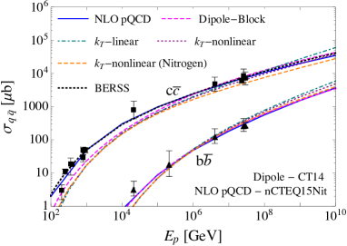
Figure 1: Total cross section for $c\bar{c}$ and $b\bar{b}$ production as a function of the incident proton energy. The results are presented for the different models described in section 2. For comparison, the previous evaluation at NLO in pQCD approach is presented as BERSS berss .

2.1 Perturbative QCD

The standard method to evaluate heavy quark production is to use the parton model in perturbative QCD (pQCD) with a collinear approximation. In the pQCD framework, the differential cross section for $q\bar{q}$ pair production is given by

$$\frac{d\sigma(pp\rightarrow q\bar{q}X)}{dx_{F}}=\int\frac{dM^{2}_{q\bar{q}}}{(x_{1}+x_{2})s}\sigma_{f_{a}f_{b}\rightarrow q\bar{q}}(\hat{s})f_{a}(x_{1},M_{F}^{2})f_{b}(x_{2},M_{F}^{2})$$ (1)

with the parton distribution function (PDF) $f_{a(b)}$, their momentum fraction $x_{1(2)}$ and the Feynman variable $x_{F}$. Momentum fractions can be expressed as $x_{1,2}=\bigl{(}(x_{F}^{2}+4M^{2}_{q\bar{q}}/s)^{1/2}\pm x_{F}\bigr{)}/2$. For the forward scattering that dominates the prompt flux, the partons from the incoming cosmic ray hadrons have the large momentum fraction $x_{1}$ while those from the target nucleus side have the small $x_{2}$.

We compute the heavy quark production cross section at next-to-leading order (NLO) to evaluate the prompt neutrino flux including the nuclear corrections. Nuclear corrections are included through the recent nuclear PDF, nCTEQ15 ncteq . For the factorization ($M_{F}$) and renormalization ($M_{R}$) scales, we use scales proportional to the transverse mass $m_{T}$, $(2.1,1.6)m_{T}$ for the central values, as experimentally constrained by the RHIC and LHC data nvf .

At the high energies where the prompt flux dominates, gluon fusion to $q\bar{q}$ is the main process, hence the essential factor is the poorly constrained gluon distribution at small-$x$. Therefore we investigate other possible approaches to the extrapolation with the resummation of large logs of $x$.

2.2 Dipole model

One of the alternative approaches is a color dipole model, which can include the parton saturation effect through the so-called dipole cross section. In the dipole model, the heavy quarks are produced through two sequential processes: a fluctuation of incoming gluon into $q\bar{q}$ pair (color dipole), and the interaction of the color dipoles with target nuclei. The dipole cross section is given by

$$\sigma^{gp\to q\bar{q}X}(x,M_{R},Q^{2})=\int dz\,d^{2}\vec{r}\,|\Psi^{q}_{g}(z,\vec{r},M_{R},Q^{2})|^{2}\sigma_{d}(x,\vec{r})\$$ (2)

with the wave function squared ($|\Psi^{q}_{g}|^{2}$) for a gluon fluctuation to a color dipole and the dipole cross section ($\sigma_{d}$) for the interaction between the dipole and the target. The $x_{F}$ differential cross section for heavy quark pair production in $pp$ collision can be written as

$$\frac{d\sigma(pp\to q\bar{q}X)}{dx_{F}}\simeq\frac{x_{1}}{x_{1}+x_{2}}g(x_{1},M_{F})\sigma^{gp\to q\bar{q}X}(x_{2},M_{R},Q^{2}=0)\ .$$ (3)

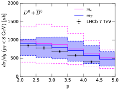
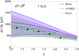
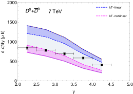
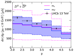
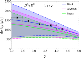
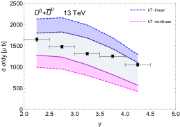
Figure 2: Rapidity distribution for $pp\to D^{0}/\bar{D}^{0}\,X$ at $\sqrt{s}=7$ TeV (upper) and at $13$ TeV (lower) from NLO perturbative QCD with nCTEQ15-01 PDFs, three dipole models with the CT14 LO gluon PDF and $k_{T}$ factorization approach. Experimental data are from the LHCb measurement lhcb .

In this work, three different dipole cross sections are used to evaluate the prompt atmospheric neutrino flux, referred to as Soyez-, AAMQS- and Block-dipole, respectively. The Soyez dipole cross section soyez is parameterized with the approximate form by iim for the solution of the BK equation, which includes saturation bk . The parameters are determined by fitting to the HERA data, and this dipole result is used in the earlier evaluation in Ref. ers . The AAMQS dipole presented in ref. aamqs is improved by including the running coupling corrections to the BK equation (rcBK). The third dipole referred to as Block-dipole blockdm is found approximately from the parameterization of the structure function $F_{2}(x,Q^{2})$ block .

For the nuclear correction in the dipole model, we use the Glauber-Gribov method, formulated as

$$\sigma_{d}^{A}(x,r)=\int d^{2}\vec{b}\,2\Biggl{[}1-\exp\Biggl{(}-\frac{1}{2}AT_{A}(b)\sigma_{d}^{p}(x,r)\Biggr{)}\Biggr{]}\ ,$$ (4)

with the impact parameter $b$. The nuclear profile function $T_{A}(b)=\int dz\rho_{A}(z,\vec{b})$ is normalized to unity, $\int d^{2}\vec{b}\,T_{A}(b)=1$. Here, we use a Gaussian distribution for nuclear density, $\rho_{A}(z,\vec{b})$.

2.3 $k_{T}$ factorization

Another possible approach is the so-called $k_{T}$ factorization scheme, which incorporates the transverse momentum of the partons. Therefore, the cross section in this scheme is expressed in terms of the $k_{T}$ dependent partonic cross section and PDFs. The cross section for this case is formulated as

$$\frac{d\sigma}{dx_{F}}(s,m_{Q}^{2})=\int\frac{dx_{1}}{x_{1}}\frac{dx_{2}}{x_{2}}\,dz\,\delta(zx_{1}-x_{F})\,x_{1}g(x_{1},M_{F})\int\frac{dk_{T}^{2}}{k_{T}^{2}}\hat{\sigma}^{\rm off}(z,\hat{s},k_{T})\,f(x_{2},k_{T}^{2})\;,$$ (5)

with collinear approximation and the integrated distributions for incoming partons and the unintegrated PDFs, which incorporates the small-x resummation for partons in the target. This is known as the hybrid formalism aabkl . In eq. (5), $g(x_{1},M_{F})$ is the integrated PDF and $f(x_{2},k_{T}^{2})$ is the unintegrated PDF. Parton saturation effect can be included through nonlinear evolution of the unintegrated PDF. We investigate both cases with ($k_{T}$-nonlinear) or without ($k_{T}$-linear) saturation effects. Nuclear effects in $k_{T}$ factorization can also be included through the unintegrated parton density, more specifically the nonlinear term in its evolution equation. The corresponding equation is presented in ref. kutak with detailed descriptions.

2.4 Total and differential cross section

Fig. 1 shows the total cross sections for the charm and bottom production from the different models described in the previous sections, perturbative QCD, dipole model and $k_{T}$ factorization. In order to incorporate the nuclear effect, we take nitrogen for the averaged air nuclei. For comparison, the earlier calculation in the perturbative QCD approach in ref. berss (BERSS) is also shown as well as the experimental data from RHIC, LHC and fixed target experiments xsection-data ; lhcb . At low energies, only perturbative QCD results agree well with the data. However, at the high energies focused in this work, all of our evaluations are consistent and have a good agreement with the data.

We also evaluate the differential cross sections in rapidity to determine the acceptable range of the scales comparing with the LHCb data lhcb . For the NLO perturbative QCD case, we take the scale variation as $(1.25,1.48)m_{T}$ and $(4.65,1.71)m_{T}$ for the lower and upper limits as guided by ref. nvf . In the left panels of fig. 2, we present the rapidity distributions for $D^{0}+\bar{D}^{0}$ production in $pp$ collisions for $2.0<y<4.5$ and $p_{T}\leq 8\rm\ GeV$ with the corresponding data from the LHCb measurements lhcb . The blue banded area presents the results evaluated with the $m_{T}$ dependent scales while the magenta dashed lines show the results with the $m_{c}=1.27\ \rm GeV$ dependent scales. The experimental data are in the narrower error bands from the scales proportional to $m_{T}$, hence we use the $m_{T}$ dependent scales for the uncertainties of the flux evaluations.

Fig. 2 also presents the predictions from the dipole models (center) and $k_{T}$ factorization (right). We have found that the differential cross sections in rapidity for $D^{0}+\bar{D}^{0}$ production from the three different dipole models are consistent with experimental data at the factorization scale, $1m_{c}\leq M_{F}\leq 4m_{c}$. For the central values shown in the plot, we take $M_{F}=2m_{c}$. For the dipole model evaluation, since there is no explicit $p_{T}$ dependence we do not apply the $p_{T}$ cut, which does not have the large effect in the results where the $p_{T}$ cut can be made.

For the $k_{T}$ factorization results, the magenta and blue bands represent the results calculated with and without a saturation effect, respectively. The band width depends on the upper limit of the integration over $k_{T}$ in eq. (5), for which is used $2.5m_{T}$ and $k_{max}$ here. The evaluations from the $k_{T}$-linear with $2.5m_{T}$ and $k_{T}$-nonlinear with $k_{max}$ gives the gray bands in the right panels of fig. 2. We use this range for the uncertainties by the scales in the prompt neutrino fluxes.

3 Prompt atmospheric neutrino fluxes

3.1 Cosmic ray fluxes

In calculating the atmospheric neutrino fluxes, the incident cosmic ray flux is one of the essential and most important factors. In many earlier calculations, the broken power law (BPL) spectrum has been used with the assumption that all cosmic rays are protons. The BPL is parameterized as $\phi_{N}(E)=1.7\ (E/{\rm GeV})^{-2.7}$ for $E<5\cdot 10^{6}$ GeV and $174\ (E/{\rm GeV})^{-3}$ for $E>5\cdot 10^{6}$ GeV. However, the recent study on the cosmic ray spectrum has provided several new parameterizations based on the models for the composition and sources of the cosmic rays. In our comprehensive work bejkrss , we used four spectra: the BPL to compare with other predictions, two parameterizations from the model for three source components gaisser and one spectrum for four source components (called GST) gst . The two spectra in gaisser is distinguished by the composition of cosmic rays from the extragalactic sources: one has a mixed composition (H3a), and the other has only protons (H3p).

In this contribution, our focus is on the effect of the different models to the prompt fluxes, therefore it would be sufficient to compare the results with only one kind of spectrum, H3p as shown in fig. 3.

3.2 Prompt muon neutrino flux

The atmospheric neutrino flux can be evaluated from the cascade equations which describe the propagation of high energy particles in the atmosphere. The coupled cascade equations for protons, hadrons and neutrinos can be solved using the approximate Z-moment method. The Z moments are the rescaled generation functions with only energy dependence, and they are associated with the production of hadrons from the interactions and their decays to neutrinos. The solutions of the coupled cascade equations can be written in terms of the Z moments for production and decay in the high energy and low energy limits. The flux of neutrinos are eventually obtained by interpolating the two approximate solutions and doing the sum over hadrons. More details for the Z-moment method are described in ref. lipari . In evaluating the muon neutrino fluxes, we take $D^{0}$, $D^{+}$, $D_{s}$, $\Lambda_{c}$ ($B^{0}$, $B^{+}$, $B_{s}$, $\Lambda_{b}$) into account for the charmed (bottom) hadrons.

Fig. 3 shows the resulting neutrino fluxes with the H3p spectrum and all the approaches introduced in section 2. We have found that the nuclear correction has different effect according to the models: about $20\%-30\%$ for the NLO pQCD, $10\%-20\%$ for the dipole models, and $30\%-50\%$ for the $k_{T}$ factorization at $10^{5}-10^{8}$ GeV. The predictions using the dipole model are larger than the fluxes from the NLO pQCD calculation all over the energy range. For the $k_{T}$ factorization case, the flux with the linear evolution is the largest above $E\sim 10^{7}$ GeV, while that from nonlinear evolution with nuclear correction is close to the lower bound of the NLO pQCD evaluation. The upper limit from the IceCube data based on 3 year observation are also presented for comparisons icecube . This IceCube limit excludes most of the dipole model results and quite constrains the upper values of the $k_{T}$ factorization results in this work. Only new predictions in the NLO pQCD and $k_{T}$ factorization with nuclear corrections are placed safely below the IceCube limit.

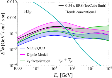
Figure 3: The prompt atmospheric neutrino fluxes from the different QCD models for the H3p cosmic ray spectrum. The upper limit from the IceCube collaboration and the conventional neutrino flux are also presented for comparison.

4 Summary

We have investigated the prompt atmospheric neutrino flux in the different frameworks for heavy quark production, NLO pQCD, three kinds of the dipole models and $k_{T}$ factorization. We set the allowed QCD scales by comparisons of the total cross sections for heavy quark production with the experimental data from RHIC and LHC nvf . We checked that the differential cross sections for $D^{0}/\bar{D}^{0}$ production with these scales are consistent with the LHCb data. The overall prompt neutrino flux is lower from NLO pQCD calculation than from the other two evaluations. The nuclear corrections are most significant in the $k_{T}$ factorization case based on the nonlinear evolution of the gluon density. In this work, we find that the nuclear corrected NLO pQCD prediction and the nuclear corrected $k_{T}$ factorization with saturation (nonlinear evolution) can safely survive from the IceCube limit based on the 3 year data. However, a new limit was recently released based on the 6 year data by IceCube after our study icecube-six , and we note that our prediction from all approaches are below this new limit.

References

- (1) M. G. Aartsen et al. [IceCube Collaboration], arXiv:1510.05223
- (2) A. Bhattacharya et al., arXiv:1607.00193
- (3) K. Kovaric K et al., Phys. Rev. D93, 085037 (2016)
- (4) R. E. Nelson, R. Vogt and A. D. Frawley, Phys. Rev. C87, 014908 (2013)
- (5) G. Soyez, Phys. Lett. B655, 32-38 (2007)
- (6) E. Iancu, K. Itakura and S. Munier, Phys. Lett. B590, 199-208 (2004)
- (7) I. Balitsky, Nucl. Phys. B463, 99-160 (1996); Y. V. Kovchegov, Phys, ReV. D60, 034008 (1999)
- (8) R. Enberg, M. H. Reno and I. Sarcevic, Phys. Rev. D78, 043005 (2008)
- (9) J. L. Albacete et al., Eur. Phys. J. C71, 1705 (2011)
- (10) C. Ewerz et al., JHEP 03, 062 (2011); Y. S. Jeong et al., JHEP 11, 025 (2014); C. Arguelles et al., Phys. Rev. D92, 074040 (2015)
- (11) M. M. Block, L. Durand and P. Ha, Phys. Rev. D89, 094027 (2014)
- (12) T. Altinoluk, N. Armesto, G. Beuf, A. Kovner and M. Lublinsky, Phys. Rev. D93, 054049 (2016)
- (13) K. Kutak and S. Sapeta, Phys. Rev. D86, 094043 (2012)
- (14) A. Bhattacharya, R. Enberg, M. H. Reno, I. Sarcevic and A. Stasto JHEP 06, 110 (2015)
- (15) UA1 Collaboration, Phys. Lett. B256 (1991) 121; LHCb Collaboration, Eur. Phys. J. C71, 1645 (2011); ALICE Collaboration, JHEP 07, 191 (2012); JHEP 11, 065 (2012); Phys. Lett. B738, 97 (2014); ATLAS Collaboration, Nucl. Phys B907, 717-763 (2016); PHENIX Collaboration, Phys. Rev. Lett. 97, 252002 (2006); Phys. Rev. C91, 014907 (2015); STAR Collaboration, Phys. Rev. D86, 072013 (2012); C. Lourenco and H. K. Wohri, Phys. Rept. 433, 127 (2006); HERA-B Collaboration, Eur. Phys. J. C52, 531 (2007);
- (16) LHCb Collaboration, R. Aaij et al., Nucl. Phys. B871, 1-10 (2013); JHEP 03, 159 (2016)
- (17) T. K. Gaisser, Astropart. Phys. 35, 801 (2012)
- (18) T. K. Gaisser, T. Stanev and S. Tilav, Front. Phys. (Beijing) 8, 748-758 (2013)
- (19) P. Lipari, Astropart. Phys. 1, 195-227 (1993)
- (20) M. G. Aartsen et al. [IceCube Collaboration], arXiv:1607.08006.