The random members of a class
Abstract.
We examine several notions of randomness for elements in a given class . Such an effectively closed subset of may be viewed as the set of infinite paths through the tree of extendible nodes of , i.e., those finite strings that extend to a member of , so one approach to defining a random member of is to randomly produce a path through using a sufficiently random oracle for advice. In addition, this notion of randomness for elements of may be induced by a map from onto that is computable relative to , and the notion even has a characterization in term of Kolmogorov complexity. Another approach is to define a relative measure on by conditionalizing the Lebesgue measure on , which becomes interesting if has Lebesgue measure 0. Lastly, one can alternatively define a notion of incompressibility for members of in terms of the amount of branching at levels of . We explore some notions of homogeneity for classes, inspired by work of van Lambalgen. A key finding is that in a specific class of sufficiently homogeneous classes , each of these approaches coincides. We conclude with a discussion of random members of classes of positive measure.
1. Introduction
The theory of algorithmic randomness for , the collection of infinite binary sequences, has been actively studied over roughly the last fifteen years. During this time, there has been some work in considering algorithmic randomness in more general settings. Random closed subsets of were introduced by Barmpalias, Brodhead, Cenzer et al in [2], and also studied by Axon [1], Diamondstone and Kjos-Hanssen [13, 12], and others. Random continuous functions were introduced by Barmpalias, Cenzer et al in [3] and have recently been studied by Culver and Porter [11]. Here, we consider only a slightly more general setting than : If we replace with some non-empty class , that is, an effectively closed subset of , is it reasonable to speak of the algorithmically random member of ? We are not simply asking here whether contains any Martin-Löf random members. For according to two standard results in algorithmic randomness, if has Lebesgue measure 0, it contains no Martin-Löf random sequences, while if has positive Lebesgue measure, it contains, up to finite modification, every Martin-Löf random sequence.
The approach we take here is to treat as a space in its own right. In particular, we consider three general approaches to defining the random members of :
-
(1)
a local approach, according to which the randomness of some is defined in terms of the behavior of initial segments of in the set of extendible nodes of , or equivalently, in terms of properties of the relatively clopen sets (in the subspace topology),
-
(2)
a global approach, according to which the randomness of some is defined in terms of properties of the entire class ; and
-
(3)
an intermediate approach, according to which the randomness of some is defined in terms of the properties of the relatively clopen sets , that is, clopen sets generated by the collection of strings of length that extend to an infinite path in .
The key finding of this study is that in sufficiently homogeneous classes, each of these approaches coincide. We also consider a number of specific examples of classes and investigate the properties of their random members.
The remainder of the paper proceeds as follows. First, in Section 2 we provide the necessary background for the remainder of the study. Next, in Section 3, we explore the local approach by formalizing the idea of randomly producing a random path of a fixed class. We also provide a number of equivalent characterizations of this initial definition. In Section 4, we define a global notion of randomness for members of a class by conditionalizing the Lebesgue measure on and compare this to the local approach. Next, we consider in Section 5 an intermediate approach first given by van Lambalgen (although he was not explicitly attempting to formalize the notion of random member of a class). This intermediate approach involves the Kolmogorov complexity of the initial segments of elements of in comparison with the number of initial segments of the same length. This approach is compared and contrasted with the local and global approaches. In Section 6, we examine various notions of homogeneous classes and show that for a sufficiently homogeneous class , the local, global, and intermediate approaches to defining random members of coincide. In Section 7, we examine the randomness of members of classes of positive measure. Conclusions are given and prospects for future work in are discussed in Section 8.
2. Background
We will assume the reader is familiar with the basics of computability theory. We fix some notation and provide some basic definitions.
2.1. Notation and preliminary definitions
denotes the collection of finite binary strings, members of which are denoted by lowercase Greek letters such as and . For , denotes the collection of binary strings of length . Given a finite string , let denote the length of . For each and each , denotes the bit of . For two strings , we say that extends and write if and for . We say that and are compatible if either or . Let denote the concatenation of and ; we will often write, for instance, and instead of and . The empty string will be denoted . For , we define to be the string obtained by flipping the last bit of , so that if , then .
denotes the collection of infinite binary sequences, which we will often identify with subsets of , viewing each sequence as a characteristic function. We will write members of as uppercase Roman letters such as and . We will write the complement of as . For , means that for , where as above, denotes the bit of . Let ; is similarly defined for and . Two sequences and may be coded together into , where and for all . More generally, given any , we can code and together via using the principal function of , i.e., the function such that if and only if is the number such that , and that of . Then we define by
That is, is obtained by coding at locations where and coding at locations where .
For a finite string , let denote . We shall refer to as the interval determined by . Each such interval is a clopen set and the clopen sets are just finite unions of intervals. A set is a tree if it is closed downwards under . For , let . A nonempty closed set may be identified with a tree where Note that has no dead ends. That is, if , then either or (or both). Note that . For an arbitrary tree , let denote the set of infinite paths through , i.e., the set of such that for every . It is well known that is a closed set if and only if for some tree . is a class, or an effectively closed set, if for some computable tree . The complement of a class is said to be a c.e. open set. This notion plays an important role in algorithmic randomness and provides a link between the two areas of study: effectively closed sets and algorithmic randomness. Note that in general, if is a class, then is a set but need not be computable. If is computable, then is said to be a decidable class. Moreover, a nonempty class need not contain any computable elements, but a nonempty decidable class certainly contains computable elements, for example the left- and right-most infinite paths. Given two closed sets and , we can define the product and the disjoint union ; if and are classes, then and are also classes. For a detailed development of classes, see [8, 10].
2.2. Computable measures and Turing functionals
By Caratheodory’s Theorem, a measure on is uniquely determined by specifying the values of on the intervals of , where for every . If in addition we require that , then is a probability measure. Hereafter, we will write as .
The Lebesgue measure is the unique Borel measure such that for all . A measure on is computable if is computable as a real-valued function, i.e., if there is a computable function (where ) such that for every and . This notion can be relativized to any oracle , yielding an -computable measure.
One family of computable measures is given by the collection of measures that are concentrated on a single computable point. If is a computable sequence, then the Dirac measure concentrated on , denoted , is defined as follows:
More generally, for a measure , we say that is an atom of or a -atom, denoted , if . Kautz [14] fully characterized the atoms of a computable measure, showing that is computable if and only if is an atom of some computable measure.
There is a close connection between computable measures and a certain class of Turing functionals. Recall that a continuous function may be defined from a function such that
-
(i)
, then , and
-
(ii)
For all , .
Moreover, a representation for a continuous function must satisfy:
-
(iii)
For all , there exists such that for every , .
We then have . The (total) Turing functionals are those which may be defined in this manner from computable . We will sometimes refer to total Turing functionals as -functionals. The partial Turing functionals are given by those which only satisfy condition (i). In this case may be ony a finite string. We set . For let be defined by
In particular, by our above convention, we have . Similarly, for we define . When is a subset of , we denote by the set . Note in particular that .
The Turing functionals that induce computable measures are precisely the almost total Turing functionals, where a Turing functional is almost total if . Given an almost total Turing functional , the measure induced by , denoted , is defined by
It is not difficult to verify that is a computable measure. That is, for any string , is the limit of the computable increasing sequence . On the other hand, since the domain of has measure 1, we also have . This shows that is also the limit of a computable decreasing sequence, and hence is computable.
Moreover, one can easily show that given a computable probability measure , there is some almost total functional such that .
Given , a function is an -computable functional if is defined in terms of an -computable functional as above. If is total and , we write .
2.3. Algorithmic randomness
Martin-Löf [16] observed that stochastic properties could be viewed as special kinds of effectively presented measure zero sets and defined a random real as one that avoids these measure zero sets. More precisely, a sequence is Martin-Löf random if for every effective sequence of c.e. open sets with , . This can be straightforwardly extended to any computable measure on by replacing the condition with . For a computable measure , the collection of -Martin-Löf random sequences will be denoted ; in the case that , we will simply write this collection as . Martin-Löf also proved the existence of a universal test , so that if and only if .
If is a universal prefix-free machine (that is, for , if and , then and for every prefix-free machine there is some such that ), then we define the prefix-free Kolmogorov complexity of to be . One of the central results in algorithmic randomness is the following.
Theorem 2.1 (Levin/Schnorr).
For each computable measure and each , is -Martin-Löf random if and only if there is some such that for all ,
We will often use the relativized version of the Levin-Schnorr theorem throughout the paper.
The following results will feature prominently in this study:
Theorem 2.2.
Let be an almost total Turing functional.
-
(i)
If then .
-
(ii)
If , then there is some such that .
We will refer to (i) as the preservation of randomness, while (ii) will be referred to as the no randomness ex nihilo principle. We will also use relativized versions of these two results.
3. A local approach to defining randomness in a class
As described in the introduction, on the local approach to defining the random members of a given class , the randomness of some is determined by the behavior of initial segments of in the set of extendible nodes of . There are several ways to make this precise. The first can be seen as a formalization of the idea of randomly producing a path through , the set of extendible nodes of .
3.1. Randomly produced paths through
Suppose we would like to randomly produce a path through for a given class . We can use the following procedure to construct a path. Having constructed a string thus far, if has only one extension in , we have no choice but to follow that extension. However, if both and are in , then we toss an unbiased coin to determine which of these extensions our path will pass through.
In the context of algorithmic randomness, we can formalize this procedure as follows. Given a Martin-Löf random , suppose that we have produced an initial segment of a path in , having thus far used as advice for some . If but for , we have no choice but to extend to . However, if both and , then we extend to .
The resulting path will have the form , where codes the levels where there is branching in along and consists of the values that are not determined by , which occur at non-branching levels of along . More precisely, we have
-
(i)
, and
-
(ii)
if , then for each , has only one extension in , namely, (where ).
Observe that . In fact, we have , which implies that there is a total -computable functional such that . We now define the randomly produced paths through as follows.
Definition 3.1.
For a class with tree of extendible nodes , the randomly produced paths through are given by the set .
Let us consider several examples.
Example 1.
-
(1)
Let . Then the randomly produced paths through are all sequences of the form for .
-
(2)
More generally, for , let . Then the randomly produced paths through are all sequences of the form for .
-
(3)
Let be a class that contains an isolated point . Then is a randomly produced path through .
This latter example appears to be an undesirable consequence of the definition of a randomly produced path through for a class , since the isolated points of a class are computable. However, we take a randomly produced path through to be one produced by tossing a coin whenever we arrive at a branching node in , counting isolated points as random is consistent with this definition.
Let be the -computable measure induced by . Then we have:
Proposition 3.2.
Let be a class. For , is a randomly produced path through if and only if .
Proof.
() If is a randomly produced path through , then for some . By the preservation of randomness theorem, it follows that .
() If , then by the no randomness ex nihilo principle, there is some such that , and hence is a randomly produced path through .
∎
Observe that the complexity of the measure is determined by the complexity of the underlying tree of extendible nodes . Thus, if is decidable, then is computable and hence so is . However, if is undecidable, then is co-c.e. but not computable, from which it follows that is merely -computable and not computable. Although algorithmic randomness with respect to a computable measure has been well-studied, the topic of algorithmic randomness with respect to an -computable measure has not been treated systematically.
3.2. An alternative characterization
Observe that if is a randomly produced path through and is not isolated in , then there is a unique such that . We can obtain an equivalent characterization of the randomly produced paths through by instead considering a -computable functional that maps onto and does not necessarily satisfy the above uniqueness condition on random sequences.
We define by means of a -computable function , which we define inductively as follows. First, we set . Next, suppose is defined for every . Then to define for , we have two cases to consider.
-
Case 1: If for each , then for each such we set .
-
Case 2: If for some (so that , then we set .
For , we define . Note that is a total -computable functional, and hence by Theorem 2.2(i) it induces a -computable measure, which we will write as .
We now prove the following.
Theorem 3.3.
Let be a class. Then is a randomly produced path through if and only if is -Martin-Löf random with respect to .
Proof.
We show inductively that and induce the same -computable measure. First, we have , and hence . Next, suppose that for every of length . For a fixed , let
That is, is the number of initial segments of that are branching nodes in , i.e., strings such that and are in . For our fixed , it follows from the definition of that there is some with such that . Hence . Similarly, there are such that , so that . We now consider two cases:
-
Case 1: Suppose that for each . Then:
-
–
For each , by definition of , we set .
-
–
For each , by definition of , we set .
It follows that for each ,
-
–
-
Case 2: Suppose that for some , and . Then:
-
–
By definition of , we set .
-
–
By definition of , we set
-
–
It follows that
and hence
It follows by induction that . Hence by Proposition 3.2, is a randomly produced path through if and only if . ∎
3.3. Initial segment complexity characterization of randomly produced paths
We can also characterize the randomly produced paths through for a given class in terms of initial segment complexity. To provide such a characterization, we need to identify a threshold so that the collection of sequences in whose initial segment complexity is above this threshold is precisely the collection of randomly produced paths through . One possibility is to define to be incompressible in if
a notion considered by van Lambalgen in [17]. However, in general, the collection of members of satisfying this definition of incompressibility does not agree with the collection of randomly produced paths through , since measures how much branching has occurred in up to strings of length , but it does not take into consideration how this branching (or lack of branching) is distributed among these strings. In particular, such an approach is at odds with the local approach to defining randomness in that we are considering here. We will look more closely at a related notion of incompressibility in Section 5.
In order to better capture the local structure of along initial segments of a sequence , we propose the following threshold. For , we define
i.e., is the number of initial segments of whose siblings are extendible (a quantity used in the proof of Theorem 3.3). Note that , and hence is a computable function if and only if is a decidable class.
Let us consider several examples of for various classes .
Example 2.
-
(1)
If , so that , then for every . Thus, we have for every random path in , which agrees with the standard definition of Martin-Löf randomness.
-
(2)
If , so that , then for every , we have , while for every of the form for some and , we have . Thus, the incompressible members of are those satisfying
which agrees with the notion of Martin-Löf randomness on as discussed in part 1 of Example 1 above.
-
(3)
Let be a class with an isolated point . Then there is some least such that . Thus there is some such that for every , . Since for every , it follows that
for every . Thus, isolated points in satisfy the definition of incompressibility.
These examples can be derived from the following result.
Theorem 3.4.
Let be a class, and let be as above. Then is a randomly produced path through if and only if
Proof.
The key observation to prove this theorem comes from comparing the function to the measure as defined in the previous subsection. Writing as , we have , where for the -computable function used in the definition of . By the definition of , this means that has initial segments whose siblings are extendible, i.e. . Thus it follows that
Now by Theorem 3.3, the randomly produced paths through are precisely the -Martin-Löf random members of with respect to . By the Levin-Schnorr Theorem for -Martin-Löf randomness with respect to , it follows that is a random path in if and only if
∎
4. A global approach to defining randomness in a class
We now turn to a global definition of the random members of a fixed class , according to which the randomness of some is defined in terms of properties of the entire class . The definition we provide here will be obtained by considering the Lebesgue measure conditional to .
4.1. Conditionalizing the Lebesgue measure
Let us first consider the case that is a class of positive Lebesgue measure. For , we define the relative measure of in is
If , we clearly need an alternative definition. Thus, we have the following definition.
Definition 4.1.
Let be a class.
-
(1)
The limiting relative measure of in is
-
(2)
The upper limiting relative measure of in is
-
(3)
The lower limiting relative measure of in is
For a class of positive measure, it follows that for every .
The reason that we consider upper and lower limiting relative measure and not merely limiting relative measure is that there are classes for which the limiting relative measure of some does not exist. The following is an example of a decidable class such that is not defined.
Example 3.
Let consist of all sequences of the form such that for all together with all sequences of the form such that for all . Then, for all , we have
Thus is not defined.
We use the tree of extendible nodes to define , as different choices of an underlying tree yield different measures. For example, suppose for any tree we define
For the set , clearly . However, consider the tree
so that . Then for all ,
and thus .
The measure is in some sense more natural than the measure considered in Section 3.
Example 4.
Let . Then , whereas and .
This example indicates the key difference between and : for each , whereas only takes into account whether and are in in distributing measure to these strings, takes into account the entire structure of above .
Note that the class from Example 3 above may be seen as the disjoint union of two classes and where and are defined but is not defined. Note that here we have , whereas , so that
Thus does not exist.
Proposition 4.2.
Let for some classes and such that is defined for each and for . Then for each string , is defined if and only if exists (including having a limit of infinity).
Proof.
Without loss of generality, let . Then for each , we have
For the first fraction above we have
For the second fraction, we have
Thus if , then we have
In particular if , then this limit will be 1. Putting these together, we see that
where again if , then . ∎
It follows from the proof that in fact, for each , exists if and only if exists and the limit exists and similarly for .
Proposition 4.3.
If and are classes such that and are both defined and , then is also defined.
Proof.
For each pair of strings of the same length and each , the number of extensions of of length in is exactly the product of the number of extensions of in of length with the number of extensions of in of length . Applying this fact to the empty string yields . Then we have
and therefore . Since intervals of the from form a basis, it follows that is defined for all intervals. ∎
Later we will consider some notions of homogeneity which will provide conditions on the class under which is defined.
4.2. Randomness with respect to the conditional measure
We now turn to the global definition of randomness in a class .
Definition 4.4.
is globally random in if .
By the relativized Levin-Schnorr theoreom, is globally random in if and only if
for all . We will make use of this characterization of global randomness in in the ensuing discussion.
The next two examples show that these measures give rise to different notions of algorithmic randomness.
Example 5.
Let . Then , so that is not random with respect to random. However, , for every , so that is random with respect to . That is, if belongs to an open set , then some such that , so that . Hence must pass every -Martin-Löf test.
Example 6.
Let . We observe that for each , has exactly elements, namely, . Now fixing , we see that has exactly elements, of which extend . It follows that
so that for all . Thus is random with respect to . On the other hand, we see that for each and that . Thus for every , so that is not -Martin-Löf random.
Example 6 shows that there are classes where the collection of -random sequences is disjoint from the collection of -random sequences. An example of such a class without isolated points is the following.
Example 7.
Let be the tree obtained by closing the set downward under and let . Note that is homeomorphic to . Now, the measure on is defined by
-
(i) , and
-
(ii)
for every . In addition, the measure on satisfies
-
(iii)
for every .
Let be the Bernoulli ()-measure on and let be the Bernoulli ()-measure on . For , every -random sequence satisfies the law of large numbers with respect to , which implies in particular that
for every -random sequence and
for every -random sequence .
Let be the Turing functional induced by the map from to given by:
Then is a measure-preserving isomorphism between and as well as between and .
Suppose that there is some that is random with respect to both and . Then setting , by the preservation of randomness, it follows that is random with respect to both and , which is impossible by our above remarks.
5. An intermediate approach to defining randomness in a class
Let us now consider the notion of initial segment complexity for members of a given class briefly considered in Subsection 3.3.
Definition 5.1.
is -incompressible if
For the previous two initial segment complexity notions we have considered, the complexity threshold for a given is determined by (i) the branching in along initial segments of and (ii) the branching in along extensions of , respectively. For -incompressible sequences, the complexity threshold is now determined by the branching along not just initial segments of but along initial segments of all strings in of length .
Recall that a sequence is complex if there is a computable, nondecreasing, unbounded function such that for all . In [7, Theorem 2.13], Binns proved that if is a class containing a complex element, then for every , there is some such that (in fact, he proved a stronger result). In particular, such a class must be uncountable. Using these facts, we can show:
Proposition 5.2.
If is a countable, decidable class, then no satisfies
Proof.
Since is decidable, then is computable and thus each -incompressible sequence satisfies
Since for , the function is computable, nondecreasing, and unbounded, it follows that such an is complex. By the above discussion, if contains any -incompressible sequence, then it contains a complex member and thus is uncountable. This contradicts the fact that is countable, and thus contains no -incompressible sequences. ∎
The following is open:
Question 5.3.
Is there an undecidable class such that no is -incompressible?
As the class from Example 6 is countable and decidable, it follows that no is -incompressible. We saw that in that case, the collection of -random sequences in is disjoint from the collection of -random sequences in . It thus follows that neither -randomness nor -randomness imply -incompressibility. As we will see in the next section, being -incompressible does not imply being a randomly produced path for some classes (see the remarks after Corollary 6.9). Moreover, Example 3 shows that -incompressibility does not imply globally randomness for all classes .
To see this, letting be the class from Example 3, one can calculate that, for ,
and hence . One can further calculate that for each and each ,
Lastly, for each and each for , we have
and
Thus, for all ,
From this it follows that is a randomly produced path through if and only if is -incompressible. As does not contain any globally random sequences, as is not defined, it follows that -incompressibility does not imply global randomness in .
Significantly, we are not aware of precisely which conditions guarantee that -incompressible sequences exist for a given class . However, in the next section we will identify several sufficient conditions for a class to contain a -incompressible member.
6. Notions of homogeneity
In this section, we explore various notions of homogeneity for classes, with the aim of showing that all of the notions of randomness for members of classes coincide for sufficiently homogeneous classes. In the next three subsections, we will first consider notions of homogeneity that have been considered in the computability-theoretic literature. In Subsection 6.4, we will introduce a new notion of homogeneity, namely additive homogeneity.
6.1. Separating set homogeneity
The first notion of homogeneity we will consider is a classic one, playing a useful role in the study of c.e. sets and the incompleteness phenomenon.
Definition 6.1.
A class is homogeneous if for every such that , if and only if for .
Recall that a class is homogeneous if and only if there are disjoint c.e. sets and such that every is a separating set for and , i.e., and . In this case, we write . As we will later introduce alternative notions of homogeneity for classes, we will hereafter refer to homogeneity in the above sense as s.s.-homogeneity (for separating set homogeneity).
Lemma 6.2.
If is an s.s. homogenous class, then for every .
Proof.
For the root node , we have and .
Now suppose the claim holds for all strings of length . Given of length , then for some of length and some . We have two cases to consider.
Case 1: If , we have . But since is homogeneous, for every of length , we must have and . Thus .
Case 2: If , we have . But since is homogeneous, for every of length , we must have for . Thus .
Hence by induction, the conclusion holds. ∎
Lemma 6.3.
If is an s.s. homogenous class, then for every .
Proof.
For , for each , we consider
Suppose that has extensions in of length . Since is homogenous, we must have for some . Thus
| (1) |
Moreover, by the homogeneity of , so that
| (2) |
Combining (1) and (2) with the fact that yields
Thus
∎
For an s.s.-homogeneous class and , by Lemmas 6.2 and 6.3, we have
for each . As an immediate consequence we have:
Theorem 6.4.
Let be an s.s.-homogeneous class. The following are equivalent for :
-
(i)
is a random path through .
-
(ii)
is -Martin-Löf random with respect to .
-
(iii)
is -incompressible.
Finally, we observe that by Lemmas 6.2 and 6.3, any s.s.-homogeneous class and any , we have . Moreover for any clopen set such that and for , we have
From this it follows that for any s.s.-homeogeneous class and any , we have , so that
This latter limit exists since the sequence is nondecreasing and bounded from below by 0.
6.2. -homogeneity and weakly -homogeneity
Generalized c.e. separating classes and their degrees of difficulty were investigated by Cenzer and Hinman [9]. For example, given four disjoint c.e. sets , consider the class such that . Now the class can be represented by a class in by letting represent by replacing with , where each 0 in is replaced by , each by , each 2 by , and each 3 by . Such a class will have the property that, for any two nodes and in of length and any string of length , if and only if . We will give a more general definition here.
Definition 6.5.
Let . Then a class is -homogeneous if for every , every , and every , if and only if . is weakly -homogeneous if, for each and each and in ,
It is easy to see that if is -homogeneous, then is weakly -homogeneous. Note further that 1-homogeneity is simply s.s.-homogeneity.
Returning briefly to the notions of product and disjoint union, we note that the disjoint union of -homogeneous classes need not be -homogeneous, as seen by Example 3. For products, the following are easy to see.
Proposition 6.6.
-
(i)
If and are both -homogeneous, then is -homogeneous.
-
(ii)
If and are both weakly -homogeneous, then is weakly -homogeneous.
If is weakly -homogeneous and is weakly -homogeneous for , then is almost weakly -homogeneous, in the following sense: For any strings and in of length , and will have an equal number of extensions of length . The details are left to the reader.
Lemma 6.7.
If is -homogeneous, then is defined for every .
Proof.
Since is -homogeneous, it follows that, for each and each ,
Now suppose where , and let be the number of extensions in of of length . Then
∎
Note that by Example 3, is not necessarily defined for weakly -homogeneous classes. In the case that is weakly -homogeneous and is defined everywhere, we have the following.
Theorem 6.8.
Let be a weakly -homogeneous class for some and suppose that is defined. Then for any , is globally random in if and only if is -incompressible.
Proof.
Suppose that is weakly -homogeneous. Then there exists a sequence of positive integers such that, for each and each , has exactly extensions in of length . Fix and a string . Then for any , has exactly elements, of which are extensions of . It follows that
Given that exists, this means that . Thus .
Corollary 6.9.
For any -homogeneous class , and any element of , is globally random in if and only is -incompressible.
Note that the class from Example 7 is 2-homogeneous and thus weakly 2-homogeneous, from which it follows that the randomly produced paths in a weakly -homogeneous class need not coincide with the -incompressible members of (in fact, as in Example 7, these two classes many even be disjoint). By the comments following Example 7, we can extend this observation to any -homogeneous class for .
6.3. Van Lambalgen’s notions of multiplicative homogeneity
In an attempt to find the broadest notion of homogeneity for classes for which the corresponding analogue of Theorem 6.4 holds, we will next consider a notion of homogeneity due to van Lambalgen [17]. The idea behind this notion is that a class is homogeneous if the amount of branching in the subclasses of does not differ too much from the amount of branching in the class as a whole.
Definition 6.10 (Van Lambalgen [17]).
Let be a class. Then is VL-homogeneous if there is some constant such that the following two conditions are satisfied:
-
(i)
for every subclass , for every and every ,
-
(ii)
for every , if we set , we have, for every ,
Given that we require the amount of branching in subclasses of to be within a multiplicative constant of the amount of branching in , we refer to these notions as notions of multiplicative homogeneity. We now prove two lemmas that simplify the verification that a given class is VL-homogeneous.
Lemma 6.11.
Suppose that condition holds for a fixed and every clopen subset of . Then holds for any closed set of .
Proof.
Given , and , let . Then and also . It follows that
from which follows. ∎
Lemma 6.12.
Suppose there is a fixed such that condition holds for any and any that together satisfy and . Then condition holds for all closed sets .
Proof.
By Lemma 6.11, it suffices to show that condition holds for all clopen . Fixing and , let and let and for . Since and are disjoint for , it follows that and are also disjoint for . Then by assumption, for each ,
It follows that
∎
As observed by van Lambalgen, the satisfaction of the condition () for a class does not rule out the possibility that has an isolated point, as () only guarantees that the branching in any subclass of does not exceed that in (up to a multiplicative constant). The additional condition () thus guarantees that VL-homogeneous classes do not contain isolated points.
Clearly itself is VL-homogeneous. We obtain many more examples from the following:
Theorem 6.13.
For any class and any , if is weakly -homogeneous, then is VL-homogeneous.
Proof.
Let be weakly -homogeneous and let be given so that for any string of length in , has exactly extensions in of length . Let and let and .
Then we have the following inequalities:
and
It follows that
Thus the condition is satisfied with constant , so that is VL-homogeneous.
Now suppose that for some string and let satisfy . Then for as above,
so that by the first inequality above,
This verifies that the condition will be satisfied by constant , for all , so that is VL-homogeneous. ∎
By the comments following Corollary 6.9, the class from Example 7 is weakly -homogeneous and thus VL-homogeneous by the above result. Since the notions of randomness from Sections 3 - 5 do not coincide in , it follows that VL-homogeneity is also not sufficient to guarantee the equivalence of these notions.
Recalling that for an s.s.-homogeneous class and any , we have as discussed previously, we would like see what conditions ensure that
exists for subclasses of a class . Recall Example 3 above, for which
does not exist. This class is weakly 4-homogeneous and therefore is vL-homogeneous by Theorem 6.13. Thus VL-homogeneity does not suffice to ensure the existence of the limit
and consequently it does not suffice to ensure that is defined everywhere. Note also that since there are random paths through that are not globally random, provides another example of a VL-homogeneous class in which the various notions of randomness for classes fail to coincide.
In the case that is defined in a VL-homogeneous class , we can show the coincidence of global randomness and -incompressibility. First we prove a lemma.
Lemma 6.14.
Let be a VL-homogeneous class.
-
(i)
If is defined, then
-
(ii)
If is not defined, we still have
and
Proof.
Let . Let . Note that , so that
Thus we can write
| (4) |
By the VL-homogeneity of and the fact that , there is some constant such that
Dividing through by yields
| (5) |
By applying (4) to (5), we get
In the case that exists, we have
In the case that is not defined, we have
from which we can derive
∎
Using part (i) of Lemma 6.14 we can now conclude the following:
Theorem 6.15.
Let be a VL-homogeneous class and suppose that is defined. Then for any , is globally random in if and only if is -incompressible.
6.4. Additive homogeneity
We lastly turn to an additive notion of homogeneity for classes.
Definition 6.16.
Let be a class. is additively homogeneous (a-homogeneous for short) if there is some constant such that for every and every ,
Recall Example 7 above, where . Here we have but , so that is not a-homogeneous. Thus -homogeneous classes need not in general be a-homogeneous.
We also have the following.
Proposition 6.17.
There is an a-homogeneous class that is not weakly -homogeneous for any .
Proof.
We construct level by level as follows. For each , we define levels
to diagonalize against weak -homogeneity. We begin by including in all strings of length 4 except for 1111 (and their initial segments). This guarantees that is not 2-homogeneous, as 00 has 4 extensions in but 11 only has 3. For each string except for 1110, we add to as well as 11100 and 11101. This has the effect that for all . We continue a similar construction from levels 6 to 9, 12 to 16, 20 to 25, etc., while adding all possible extensions between these levels. Clearly, the resulting class is a-homogeneous (with constant ) and fails to be weakly -homogeneous for all . ∎
This example also shows that so need not be defined for a-homogeneous classes.
Despite the fact that is not defined for every a-homogeneous class , we still get a stronger result concerning the relationship between the various notions of randomness for classes than we do for weakly -homogeneous classes and VL-homogeneous classes, which we now show. First we prove a useful combinatorial lemma.
Lemma 6.18.
Let be a class and let and .
-
(i)
If every extension in satisfies , then has at least extensions in .
-
(ii)
If every extension in satisfies , then has exactly extensions in .
Proof.
(i) For , given of length that satisfies , there must be some satisfying such that . Hence there is some in , yielding two extensions of of length .
Suppose the claim holds for all and and some fixed ; we will show it similarly holds for . Suppose further that every extension of length satisfies . Let be the shortest incompatible extensions of . Then for , every extension of of length satisfies . Thus by the inductive hypothesis, has at least extensions of length for . Thus has at least extensions of length .
The proof of (ii) is nearly identical. ∎
Lemma 6.19.
Let be an a-homogeneous class. Then there is some such that for every and every ,
Proof.
Let satisfy for every and every . For a fixed , let . Given with , set , and let be largest such that (if , ). By the minimality of , it follows that every extension of satisfies . By Lemma 6.18(i), , and hence , has extensions in . Thus
| (6) |
Next, let In the most extreme case, for every we have . Applying the Lemma 6.18(ii) to , this implies that has extensions in . Thus,
| (7) |
Combining (6) and (7) and taking logarithms yields
| (8) |
Given , it follows from our hypothesis that
| (9) |
From (8) and (9) we can conclude
∎
A careful reading of the proof of Lemma 6.19 shows that each step can be reversed, so that we have the following.
Corollary 6.20.
A class is a-homogeneous if and only if there is some such that for every and every ,
Theorem 6.21.
Let be an a-homogeneous class. Then is a randomly produced path through if and only if is -incompressible.
Next we have:
Theorem 6.22.
Every a-homogeneous class is VL-homogeneous.
Proof.
Let be an a-homogeneous class. By Lemma 6.12 it suffices to show that for all , all , and , there is some such that
Fix such and . Since is a-homogeneous, by Lemma 6.19, there is some such that
from which it follows that
| (10) |
Now let
and
Then since every extension of in satisfies , by Lemma 6.18(i), we have . Moreover, since every extension of in satisfies , in the most extreme case, we have for all such . It then follows from Lemma 6.18(ii) that . Given that this is the most extreme case, it follows that in general. Summing up, we have
| (11) |
Note by a-homogeneity, it follows that , which combined with (11) yields
| (12) |
Next, if , then by a-homogeneity and the definition of and , we have
| (13) |
Again, by a-homogeneity, we have
from which it follows that
Combined with (13), this yields
and hence
| (14) |
since . Now we have by (10) and (14)
which simplifies to
| (15) |
Then by the second inequality in (12) and the first inequality in (15)
Similarly, by the first inequality in (12) and the last inequality in (15)
which, when setting , establishes the conclusion. ∎
Theorem 6.23.
Let be an a-homogeneous class and suppose that is defined for all . Then for , the following are equivalent:
-
(a)
is a randomly produced path through .
-
(b)
is -incompressible.
-
(c)
is globally random in .
In the case that is not defined for an a-homogeneous class , we still can prove the following:
Theorem 6.24.
Let be an a-homogeneous class. Then for , the following are equivalent:
-
(a)
is a randomly produced path through .
-
(b)
is -incompressible.
-
(c)
for all .
-
(d)
for all .
Proof.
The relationship between the various notions of homogeneity can be summed up in Figure 1 (where the absence of an implication arrow means that implication in question does not hold). In addition, the main properties of the various notions of homogeneity, whether is always defined and whether all randomness notions coincide in the case that is defined, are summed up in Table 1
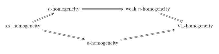
| always defined | all randomness notions coincide | |
|---|---|---|
| s.s. homogeneity | Y | Y |
| -homogeneity | N | N |
| weak -homogeneity | N | N |
| a-homogeneity | N | Y |
| VL-homogeneity | N | N |
7. classes of positive measure
We conclude with a discussion of notions of random members of certain classes of positive measure. We begin with a basic fact.
Lemma 7.1.
If is a class of positive measure, then satisfies the condition () in the definition of VL-homogeneity.
Proof.
Let . We claim that for every ,
To show this, we will prove that for every ,
| (16) |
Suppose not. Then there are such that
Then, noting that for any class , we have for every , it follows that
which contradicts our original assumption. The conclusion now follows from (16) and the fact that
∎
For an example of a class of positive measure that fails to satisfy condition (), consider , where and .
We now can consider the random members of various classes of positive measure. Our discussion makes use of the notion of lower dyadic density. We define the lower dyadic density of at to be
We note that the term “lower density” is used in the context of effectively closed subsets of , while “lower dyadic density” is used in the contexts of effective closed subsets of . The lower density of a point in a given effectively closed class has been of considerable interest recently. See, for instance, [5], [4], and [15].
Recall that is simply the collection of sequences that are -Martin-Löf random relative to .
Theorem 7.2.
Let be a class of positive measure. For of positive lower dyadic density in , the following are equivalent:
-
(i)
;
-
(ii)
for all ;
-
(iii)
for all .
Proof.
(i) (ii) Since has positive lower dyadic density in , there is some and some such that for all ,
which implies that for almost every . From this we can conclude that
and thus
for every . Then by the relativized Levin-Schnorr theorem,
(ii)(iii) Since , it follows from Lemma 7.1 that satisfies condition () in the definition of VL-homogeneity. By the proof of Lemma 6.14 , the satisfaction of condition () implies that
for some . This implies that
for every , from which the desired implication immediately follows.
(iii)(i) Let satisfy . For , since , it follows that . Thus and hence
from which it follows that is -random.
∎
By Propositions 7.7 and 7.8 below, we need an additional hypothesis on to include the property of being a randomly produced path through with the conditions (i)-(iii) in Theorem 7.2.
A number of corollaries follow immediately from Theorem 7.2.
Corollary 7.3.
Let be a decidable class. For of positive lower dyadic density in , the following are equivalent:
-
(i)
is Martin-Löf random;
-
(ii)
for all ;
-
(iii)
for all .
Corollary 7.4.
Let be a class of positive measure such that . For , the following are equivalent:
-
(i)
is 2-random, i.e., ;
-
(ii)
for all ;
-
(iii)
for all .
Proof.
It follows from work of Bienvenu et al. in [5] that if is 2-random and , has lower density 1 in ; moreover, Khan and Miller [15] showed that for Martin-Löf random sequences, having lower density 1 and lower dyadic density one are equivalent. Thus satisfies the hypothesis of Theorem 7.2 and the conclusion follows. ∎
Corollary 7.5.
Let , where is a universal Martin-Löf test. Then for , the conditions (i)-(iii) in Corollary 7.4 are equivalent.
Proof.
Since is co-c.e. and for some (such as the leftmost path of ), has diagonally non-computable (DNC) degree. That is, computes a total function such that for all , if then . By Arslanov’s Completeness Criterion, the only c.e. DNC degree is the complete one, hence . The result thus follows by applying Corollary 7.4. ∎
The branching number function played an important role in Section 6 in characterizing the randomness of members of classes which satisfied various forms of homogeneity. We now investigate the connection between density in a class of positive measure and the function . First we prove the following general lemma about lower density and in an arbitrary class .
Lemma 7.6.
Let be a class of positive measure and let . Suppose that for some . Then for all .
Proof.
Since
there is some such that for all
Suppose now that there is some such that for every we have but . For , observe that implies that and thus for every ,
| (17) |
It follows from (17) that for every ,
| (18) |
Applying (18) times to yields
| (19) |
Next, by choice of we have
| (20) |
Combining (19) and (20) yields
which is clearly impossible. Thus, for each and each block of values , there must be some such that both and . Thus there is some sufficiently large such that for every . ∎
Proposition 7.7.
Let be a class of positive measure. If , then is a randomly produced path through . In particular, if , then every 2-random is a randomly produced path through .
Proof.
Since for every and , we have
Thus is a randomly produced path through . ∎
Proposition 7.8.
Let be a class of positive measure. If is a randomly produced path through of lower dyadic density in strictly greater than 1/2, then . In particular, if , then every randomly produced path through of lower dyadic density in strictly greater than 1/2 is 2-random.
Proof.
Since has has lower dyadic density strictly greater than 1/2 in , it follows from Lemma 7.6 that for every . Then
Thus . ∎
Note that the density condition is necessary: Let and be a class containing no 1-randoms (such as or ). Then not every randomly produced path through is in (i.e., those randomly produced paths extending the string 1).
Corollary 7.9.
Let be a class of positive measure. For any with lower dyadic density in strictly greater than 1/2, the following are equivalent:
-
(i)
;
-
(ii)
for all ;
-
(iii)
for all ;
-
(iv)
is a randomly produced path through .
One interesting consequence of this result is that if , where is a universal Martin-Löf test, then if has lower dyadic density in strictly greater than 1/2 and is not 2-random, then is not a random member of (according to any of our definitions). As shown by Bienvenu et al. [4], there are sequences that have lower density 1 in every effectively closed class containing (which, by the result of Khan and Miller [15] referenced above, also holds of lower dyadic density) but which are not 2-random (they exhibit a low Oberwolfach random sequence, where Oberwolfach randomness is a notion of randomness that guarantees lower density 1). However, the following question remains open.
Question 7.10.
If is a class of positive measure, are there randomly produced paths through with lower dyadic density at most 1/2? In particular, if , is a randomly produced path through if and only if is 2-random?
8. Conclusion and future work
In this paper, we define some notions of randomness for members of a given closed set . may be defined as the set of infinite paths through a tree with no dead ends. We define a natural mapping from into which uses an input to determine which branch to follow in , and say that is randomly produced path through if for some Martin-Löf random sequence . The map induces a measure on and we show that is a randomly produced member of if and only if it is random with respect to this measure. We give an alternative mapping and show that randomness with respect to the measure induced by is equivalent to being randomly produced. The branching number is defined to be the number of initial segments of such that both and are in . It is shown that is a randomly produced element if and only if , which is a notion of incompressibility.
We define a limiting relative measure . This will be the usual relative Lebesgue measure if but otherwise may not exist. We say that is globally random if it is -Martin-Löf random with respect to the measure . We say that is -incompressible if .
Several notions of homogeneity for classes are developed in part to find conditions under which is defined and to characterize randomness with respect to . The closed set is said to be s.s.-homogeneous if for every of the same length, for . We show that if is s.s.-homogeneous, then is defined and for all , is a randomly produced path if and only if is globally random in if and only if is incompressible. This result is extended to -homogeneous classes , where all nodes of length have the same extensions of length in . We also say that is weakly -homogeneous if each node in of length has the same number of extensions of length .
Van Lambalgen develop a notion of multiplicative homogeneity for a class , which concerns the relative number of branches in any subclass of . We show that any weakly -homogeneous class is VL-homogeneous; we call this notion VL-homogeneity. We show that if is defined for a VL-homogeneous class, then from which it follows that is globally random in if and only if is -incompressible.
For a final notion of homegeneity, we say that is additively homogeneous if there is a constant such that for all and all of length , . We show that a member of an additively homogeneous class is a randomly produced path through if and only if it is -incompressible. We further show that every additively homogeneous class is VL-homogeneous. From this it follows that if , then each of the main notions of randomness coincide in .
Lastly, we examine the random members of classes of positive measure, isolating conditions under which all of the main notions of randomness coincide for such classes.
In future work we plan to investigate the random members of deep classes [6] (such as the collection of completions of Peano arithmetic and the collection of -valued diagonally non-computable functions, which is an s.s.-homogeneous class), thin classes, computably perfect classes, and ranked classes.
References
- [1] Logan M Axon. Martin-Löf randomness in spaces of closed sets. The Journal of Symbolic Logic, 80(02):359–383, 2015.
- [2] G. Barmpalias, P. Brodhead, D. Cenzer, S. Dashti, and R. Weber. Algorithmic randomness of closed sets. J. Logic and Computation, 17:1041–1062, 2007.
- [3] G. Barmpalias, P. Brodhead, D. Cenzer, J.B. Remmel, and R. Weber. Algorithmic randomness of continuous functions. Archive for Mathematical Logic, 46:533–546, 2008.
- [4] Laurent Bienvenu, Noam Greenberg, Antonín Kučera, André Nies, and Dan Turetsky. Coherent randomness tests and computing the -trivial sets. J. Eur. Math. Soc. (JEMS), 18(4):773–812, 2016.
- [5] Laurent Bienvenu, Rupert Hölzl, Joseph S. Miller, and André Nies. Denjoy, Demuth and density. J. Math. Log., 14(1):1450004, 35, 2014.
- [6] Laurent Bienvenu and Christopher P. Porter. Deep classees. The Bulletin of Symbolic Logic, pages 249–286, 2016.
- [7] Stephen Binns. classes with complex elements. The Journal of Symbolic Logic, 73(04):1341–1353, 2008.
- [8] D. Cenzer and J.B. Remmel. Effectively closed sets. To Appear.
- [9] Douglas Cenzer and Peter G. Hinman. Degrees of difficulty of generalized r.e. separating classes. Archive for Mathematical Logic, 45:629–647, 2008.
- [10] Douglas Cenzer and Jeffrey B Remmel. classes in mathematics. Studies in Logic and the Foundations of Mathematics, 139:623–821, 1998.
- [11] Quinn Culver and Christopher P Porter. The interplay of classes of algorithmically random objects. Journal of Logic and Analysis, 7, 2016.
- [12] D. Diamondstone and B. Kjos-Hanssen. Martin-Löf randomness and galton-watson processes. Annals of Pure and Applied Logic, 163:519–529, 2012.
- [13] David Diamondstone and Bjørn Kjos-Hanssen. Members of random closed sets. In Conference on Computability in Europe, pages 144–153. Springer, 2009.
- [14] Steven M. Kautz. Degrees of random sets. PhD thesis, Cornell University, 1991.
- [15] Mushfeq Khan. Lebesgue density and classes. J. Symb. Log., 81(1):80–95, 2016.
- [16] P. Martin-Lof. The definition of random sequences. Information and Control, 9:602–619, 1966.
- [17] Michiel Van Lambalgen. Random Sequences. PhD thesis, University of Amsterdam, 1987.