On-line detection of qualitative dynamical changes in nonlinear systems: the resting-oscillation case

Abstract

Motivated by neuroscience applications, we introduce the concept of qualitative detection, that is, the problem of determining on-line the current qualitative dynamical behavior (e.g., resting, oscillating, bursting, spiking etc.) of a nonlinear system. The approach is thought for systems characterized by i) large parameter variability and redundancy, ii) a small number of possible robust, qualitatively different dynamical behaviors and, iii) the presence of sharply different characteristic timescales. These properties are omnipresent in neurosciences and hamper quantitative modeling and fitting of experimental data. As a result, novel control theoretical strategies are needed to face neuroscience challenges like on-line epileptic seizure detection. The proposed approach aims at detecting the current dynamical behavior of the system and whether a qualitative change is likely to occur without quantitatively fitting any model nor asymptotically estimating any parameter. We talk of qualitative detection. We rely on the qualitative properties of the system dynamics, extracted via singularity and singular perturbation theories, to design low dimensional qualitative detectors. We introduce this concept on a general class of singularly perturbed systems and then solve the problem for an analytically tractable class of two-dimensional systems with a single unknown sigmoidal nonlinearity and two sharply separated timescales. Numerical results are provided to show the performance of the designed qualitative detector.

1 Introduction

In neurosciences, to detect on-line the current activity type of a neuron (spiking, bursting etc.) or of a population of neurons (resting, ictal, interictal, slow/fast oscillations etc.) is of fundamental importance. For epilepsy for instance, such algorithms could be used to detect or even predict seizures. It seems that this problem is very challenging from a control-theoretic viewpoint for several reasons. First, disparate combinations of biophysical parameters are known to lead to the same activity pattern at the cellular level [2], and the same degenerated parametrization property propagates at the neuronal circuit level [3]. Second, biophysical parameters change smoothly over time but by doing so they induce sharp, almost discontinuous, transitions between qualitatively different activity types (spiking or bursting, healthy or epileptic, etc.) at the crossing of critical parameter sets. Third, the few available models are often subject to large uncertainties. As a consequence, quantitative modeling and fitting of experimental neuronal data generally constitute an ill-posed problem: a new viewpoint on the problem is needed, which is the purpose of this work.

A first major point is to extract the ruling parameters governing neuronal dynamics and their critical values. In spite of the nonlinear, degenerate structure of the biophysical parameter space, neuronal systems typically exhibit only a few distinct qualitative behaviors. For instance, the activity can be classified as resting, spiking, bursting at the single cell level, and as resting, low amplitude/high frequency, high amplitude/low frequency oscillations at the network level. Predicting the structure of the critical parameter set, where switches in behavior occur, remains an open problem in general. Recently, based on singularity and singular perturbation theories, it was shown that the quantitative parameter space of biophysical neuronal models can be mapped to a small number of lumped parameters. The lumped parameters define low-order polynomial models, capturing the qualitative neuronal behavior at the single cell level [4, 5]. The resulting geometric framework allows a local, qualitative sensitivity analysis of neuronal dynamics [5, 6], which predicts the effect of biophysical parameter variations on the qualitative behavior and the qualitative shape of the critical parameter set. Motivated by the above considerations and inspired by the qualitative sensitivity analysis in [5, 6], our first objective is to extract analytically the parameters that rule the activity type of a highly uncertain, redundantly parametrized system and then to detect on-line the activity type and whether a dynamical change is likely to occur.

We formulate these ideas on a general class of nonlinear singularly perturbed control systems that embrace, for instance, the Hodgking-Huxley model for neuronal spiking [7] and the Wilson-Cowan model for neuronal population activity [8]. The singularly perturbed nature of the model is justified by neuronal biology, where sharply separated timescales govern the neuronal dynamics [5, 4, 6]. Because the proposed problem is very general and challenging, we then focus on solving it for a two dimensional class of nonlinear systems with a single unknown sigmoidal nonlinearity and two sharply separated timescales. This class of systems captures the qualitative features of the center manifold reduction of higher-dimensional biophysical models, as we explain. In order to cope with the peculiarities of neuronal dynamics, we assume that the exact functional form of the sigmoid nonlinearity is unknown as well as the exact timescale separation. We firstly show that, independently of the particular expression of the sigmoid nonlinearity, the system exhibits either global exponential stability (resting) or relaxation oscillations depending on a single ruling parameter. Guided by singularity theory [9, 10], we subsequently design an on-line qualitative detector that infers the activity type of the system and determines whether a qualitative dynamical transition is close to occur. By qualitative, we mean that the detector neither needs to quantitatively fit any model nor to asymptotically estimate any parameter. Because activity transitions are governed by bifurcations of the underlying vector field, the detection problem put forward here is closely related to the problem of steering a system toward an a priori unknown bifurcation point [11, 12].

The main contributions of the present work are summarized as follows.
$\bullet$Inspired by neurosciences, we formulate the problem of detecting on-line qualitative changes in nonlinear systems for which an exact model is not available.
$\bullet$We provide a solution for a class of two-dimensional nonlinear systems, to detect whether the system is close to a transition between resting and oscillatory activity. The stability and the robustness of the detector are ensured via Lyapunov techniques and geometric singular perturbation arguments.
$\bullet$We provide numerical evidences that the same detector performs well when tested on a classical, high dimensional, biophysical neuronal model of resting and spiking oscillations due to Hodgkin and Huxley [7].

The paper is organized as follows. In Section 2, we first formulate the idea on a general nonlinear systems. We then introduce and analyze a class of singularly perturbed nonlinear systems with a single unknown sigmoidal nonlinearity. In Section 3, we design and analyze the qualitative detector for the latter. Numerical simulations are presented in Section 4. Section 5 concludes the paper. The proofs are given in the appendix.

Notation. Let $\mathbb{R}_{\geqslant 0}:=[0,\infty)$, $\mathbb{R}_{>0}:=(0,\infty)$, and $\mathbb{N}:=\{1,2,\ldots,\}$. The usual Euclidean norm is denoted by $|\cdot|$. For $x,y,z\in\mathbb{R}$, the vector $[x,y,z]^{\top}$ is denoted by $(x,y,z)$. For a function $h:\mathbb{R}_{\geqslant 0}\to\mathbb{R}^{n}$, the associated infinity norm is denoted by $\|h\|_{[0,\infty)}=\sup_{s\in[0,\infty)}|h(s)|$, when it is well-defined. We use $\text{sgn}(x)$ to denote the sign function from $\mathbb{R}$ to $\{-1,0,1\}$ with $\text{sgn}(0)=0$. For any function $f:\mathbb{R}\to\mathbb{R}$, we denote the range of $f$ as $f(\mathbb{R})=\{z:z=f(x)\;\text{for some}\;x\in\mathbb{R}\}$. Let $A,B$ be two non-empty subsets in $\mathbb{R}^{n}$, their Hausdorff distance is noted by $d_{H}(A,B)=\max\{\sup_{a\in A}\inf_{b\in B}|a-b|,\;\sup_{b\in B}\inf_{a\in A}|a-b|\}$. The point to set distance from $p\in\mathbb{R}^{n}$ to $A\subseteq\mathbb{R}^{n}$ is denoted by $|p|_{A}=\inf\limits_{a\in A}|p-a|$.

2 Problem statement

2.1 General formulation

We first introduce the main ideas on the following general class of nonlinear singularly perturbed systems

$$[left=\!\!\!\!\empheqlbrace\,]\dot{x}_{f} =f(x_{f},h_{s}(x_{s}),\alpha,u),$$ (1a)

$$\dot{x}_{s} =\varepsilon g(h_{f}(x_{f}),x_{s}),$$ (1b)

$$y =(h_{f}(x_{f}),h_{s}(x_{s})),$$ (1c)

where $x_{f}\in\mathbb{R}^{n}$, $x_{s}\in\mathbb{R}^{m}$ are the state variables, $\alpha\in\mathbb{R}^{p}$ is an unknown parameter vector, $u\in\mathbb{R}$ is a constant input, $0<\varepsilon\ll 1$ is an unknown parameter, $h_{s}:\mathbb{R}^{m}\to\mathbb{R}$, $h_{f}:\mathbb{R}^{n}\to\mathbb{R}$ and all functions are smooth.

System (1) is said to be redundantly parametrized if it depends on numerous parameters, i.e. $p\gg 1$, but the possible qualitatively distinct dynamical behaviors are only a few. Parametric redundancy naturally arises under two conditions: timescale separation and the presence of an organizing center, as explained below.

System (1) evolves according to two time scales, since $\varepsilon$ is small. Under suitable stability and monotonicity conditions of the fast dynamics (see e.g. [13]), the trajectories of the fast variable $x_{f}$ are forced toward its instantaneous quasi-steady state $x_{f}^{*}(t)$, which is defined as follows. For all $t\in\mathbb{R}_{\geq 0}$, $\alpha\in\mathbb{R}^{p}$, $u\in\mathbb{R}$, let $x_{s}(t)$ be the slow state at time $t$. Then $x_{f}^{*}(t)$ is a solution of the quasi-steady state equation $f(x_{f}^{*}(t),h_{s}(x_{s}(t)),\alpha,u)=0$, and the fast output $y_{f}=h_{f}(x_{f})$ will change accordingly. Now, for $u$ fixed, define the map $G:\mathbb{R}^{n+1}\times\mathbb{R}\times\mathbb{R}^{p}\to\mathbb{R}^{n+1}$ as

$$G(x,\lambda,\alpha):=\begin{bmatrix}f(x_{f},\lambda,\alpha,u)\\ y_{f}-h_{f}(x_{f})\end{bmatrix},$$

where $x=(x_{f},y_{f})$ and $\lambda$ is the bifurcation parameter. For system (1) to be redundantly parameterized, we assume that the map $G$ is organized by a $k$-codimensional singularity, with $k\ll p$, in the sense of [9, Section III.1]. This means that the qualitative shape of the graph of the, possibly multivalued, mapping $\lambda\mapsto x_{f}$ defined by solving the equation $G(x,\lambda,\alpha)=0$ is given by one of the persistent bifurcation diagrams [9, Sections III.5,6] in the universal unfolding of the organizing singularity. This shape is exactly what determines the quasi-steady state evolution of the fast variable. Under suitable stability and monotonicity properties of the slow dynamics, (for instance that they provide slow adaptation - negative feedback - on the fast dynamics), it follows that the possible qualitative dynamic output behaviors of system (1) are fully determined by the persistent bifurcation diagrams of the organizing singularity. Hence, since $k\ll p$, the possible different persistent bifurcation diagrams, and therefore the possible output behaviors are much less than the number of model parameters: parametric redundancy occurs.

When system (1) exhibits parametric redundancy, we do not need to know the full vector of parameters $\alpha\in\mathbb{R}^{p}$ to detect what is the current dynamic behaviour of the system and whether a qualitative change is prone to appear. The projection of $\alpha$ onto the $k$-dimensional unfolding space of the organizing suffices to determine the model behavior. The sensitivity analysis proposed in [4] is fully based on this idea. In this paper, we explore this viewpoint to formulate the following qualitative detection problem: Let $f$, $g$, $h_{f}$, $h_{s}$ be unknown. Let the organizing singularity be known. Let the slow and fast output be measurable. Let the dimension $p$ of the parameter space be unknown. Can we detect on-line in which region of the organizing singularity unfolding space the parameter vector lies and whether this vector is approaching a transition variety, where a qualitative dynamical transition occurs?

This problem is new, general and very challenging. That is the reason why we solve it for a particular yet relevant class of systems of the form of (1) in the following.

2.2 A tractable class of systems

In the following, we concentrate on systems of the form

$$[left=\!\!\!\!\empheqlbrace\,]\dot{x}_{f} =-x_{f}+S(\beta x_{f}+u-x_{s}),$$ (2a)

$$\dot{x}_{s} =\varepsilon(x_{f}-x_{s}),$$ (2b)

where $x_{f},x_{s}\in\mathbb{R}$ are the state variables, $\beta\in\mathbb{R}$ is an unknown parameter, $u\in\mathbb{R}$ is the input, which is assumed to be known and constant, and $0<\varepsilon\ll 1$ is small unknown parameter. The mapping $S:\mathbb{R}\to\mathbb{R}$ is an unknown sigmoid function, which is assumed to satisfy the following properties.

Assumption 1.

The following properties holds.
a$)$ $S$ is smooth on $\mathbb{R}$.
b$)$ $S(0)=0$.
c$)$ $S^{\prime}(a)>0$ for all $a\in\mathbb{R}$ (monotonicity), and ${\rm argmax}_{a\in\mathbb{R}}S^{\prime}(a)=0$ (sector-valued).
d$)$ ${\rm sgn}\left(S^{\prime\prime}(a)\right)=-{\rm sgn}(a)$ for all $a\in\mathbb{R}$.$\hfill\Box$

Standard sigmoid functions such as $a\mapsto c_{1}\tanh(c_{2}a)$, $a\mapsto\frac{c_{1}}{1+e^{-c_{2}a}}-\frac{c_{1}}{2}$, $a\mapsto e^{-e^{-c_{1}a}}-c_{2}$ with $c_{1},c_{2}\in\mathbb{R}_{>0}$, verify Assumption 1. Moreover, when $S=\sum\limits^{n}_{i=1}S_{i}$ where $S_{1},\cdots,S_{i}$ with ($i\in\mathbb{N}$) are sigmoid functions satisfying Assumption 1, then so does $S$.

Due to the small parameter $\varepsilon$, system (2) evolves according to two time scales. We follow the standard approach of singular perturbation theory [14, 15] to decompose system (2) into two subsystems, which represent the fast dynamics and the slow dynamics, respectively, called the layer and the reduced subsystems. By setting $\varepsilon=0$ in (2b), we obtain the layer dynamics

$$[left=\empheqlbrace\,]\dot{x}_{f} =-x_{f}+S(\beta x_{f}+u-x_{s}),$$ (3a)

$$\dot{x}_{s} =0.$$ (3b)

Because of (3b), the variable $x_{s}$ can be treated as a parameter in (3a).

To account for the slow variations of $x_{s}$, we rescale the time as $\tau=\varepsilon t$, hence $\frac{d}{dt}=\varepsilon\frac{d}{d\tau}$. Then, system (2) becomes

$$[left=\empheqlbrace\,]\varepsilon x^{\prime}_{f} =-x_{f}+S(\beta x_{f}+u-x_{s}),$$ (4a)

$$x^{\prime}_{s} =x_{f}-x_{s},$$ (4b)

where $\prime$ stands for $\frac{d}{d\tau}$. Setting $\varepsilon=0$ in (4a), we obtain the reduced dynamics

$$[left=\empheqlbrace\,]0 =-x_{f}+S(\beta x_{f}+u-x_{s})$$ (5a)

$$=:F_{f}(x_{f},u-x_{s},\beta),$$

$$x^{\prime}_{s} =x_{f}-x_{s}=:F_{s}(x_{f},x_{s}).$$ (5b)

The reduced dynamics evolves in the slow time $\tau$ and is an algebro-differential equation. In particular it defines a one-dimensional vector field over the critical manifold rCl S^0_u,β&:={(x_s,x_f)∈R^2: F_f(x_f,u-x_s,β)=0}. The critical manifold $S_{u,\beta}^{0}$ depends on $u$ and $\beta$. However, since we assume $u$ and $\beta$ constant, for simplicity we omit the index $u$ and $\beta$ in the rest of the paper. The critical manifold will therefore simply be denoted by $S^{0}$. The idea behind singular perturbations is that dynamics (2) are well approximated by layer dynamics far from $S^{0}$ and by trajectories of the reduced dynamics close to $S^{0}$. The shape of $S^{0}$ therefore plays a key role in determining the behavior of system (2).

Let

$$\beta_{c}:=\frac{1}{S^{\prime}(0)},$$ (6)

which is well-defined and strictly positive according to item c$)$ of Assumption 1. The parameter $\beta_{c}$ is crucial in shaping the critical manifold $S^{0}$, as illustrated in Figure 1. For $\beta<\beta_{c}$ the shape of $S^{0}$ is given by graph of a monotone decreasing function. Whereas for $\beta>\beta_{c}$ the shape of $S^{0}$ is $S$-shaped. We emphasize that $\beta_{c}$ is unknown since so is the sigmoid function $S$.

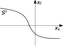
(a) $\beta<\beta_{c}$

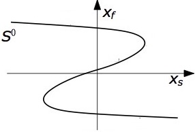
(b) $\beta>\beta_{c}$

Figure 1: Qualitative shape of the critical manifold $S^{0}$.

The qualitative properties of the critical manifold fully determine the model dynamical behaviors, as formalized in the next proposition, whose proof can be found in [16].

Proposition 2.1.

Consider system (2), the following holds.
1) For any $\beta-\beta_{c}<0$ and any constant input $u$, there exists $\bar{\varepsilon}>0$ such that, for all $\varepsilon\in(0,\bar{\varepsilon}]$, system (2) has a globally exponentially stable fixed point. Moreover, all trajectories converge in an $\mathcal{O}(\varepsilon)$-time to an $\mathcal{O}(\varepsilon)$-neighborhood of the critical manifold $S^{0}$ defined in (5).
2.a) For all $0<\beta-\beta_{c}<1$, there exists $\bar{u}>0$, such that, for any constant input $u$ in $(-\bar{u},\bar{u})$, there exists $\bar{\varepsilon}>0$ such that, for all $\varepsilon\in(0,\bar{\varepsilon}]$, system (2) possesses an almost globally asymptotically stable and locally exponentially stable periodic orbit $P^{\varepsilon}$.
2.b) Let $\beta,\bar{u},u,\bar{\varepsilon},\varepsilon$ be as in item 2.a), and let $T^{\varepsilon}$ be the period of $P^{\varepsilon}$ and $p:\mathbb{R}\to P^{\varepsilon}$, with $p(t)=p(t+T^{\varepsilon})$ for all $t\in\mathbb{R}$, be a periodic solution of (2). Let $P^{0}$ be the singular limit of $P^{\varepsilon}$. The Hausdorff distance between $P^{\varepsilon}$ and $P^{0}$ verifies $d_{H}(P^{\varepsilon},P^{0})=\mathcal{O}(\varepsilon^{2/3})$. Moreover, for all $t_{0}\in\mathbb{R}$, there exists $\delta T^{\varepsilon}\subset[t_{0},t_{0}+T^{\varepsilon})$ and $|\delta T^{\varepsilon}|=\mathcal{O}(\varepsilon)T^{\varepsilon}$, such that $|p(t)-S^{0}|<\mathcal{O}(\varepsilon)$ for all $t\in[t_{0},t_{0}+T^{\varepsilon})\setminus\delta T^{\varepsilon}$. $\hfill\Box$

Proposition 2.1 shows that system (2) either has a globally exponentially stable fixed point (item 1)), which we call the resting activity, or almost all its solutions converge to a limit cycle (item 2)), in which case we talk of oscillating activity. The nature of the activity is solely determined by the sign of $\beta-\beta_{c}$, independently of the particular expression of $S$.

Remark 2.2.

Proposition 2.1 states stability results for $\beta<\beta_{c}+1$. When $\beta>\beta_{c}+1$, system (2.1) exhibits three equilibria, two of which are asymptotically stable and one is unstable. Then trajectories converge to the two stable equilibria.

Remark 2.3.

Higher-dimensional control systems of the form (1) may be reduced to the simpler lower-dimensional system (2) via center manifold reduction [18]. We sketch the ideas as follows. The transition from globally asymptotically stable fixed point to almost globally asymptotically, locally exponentially stable oscillations in model (2) is via a Hopf bifurcation, as it can easily be verified by linearization at the origin (for $u=0$). Assume that the same bifurcation exists in the full model (1). Then, close to this bifurcation, by the center manifold theorem, the dynamics of model (1) can be reduced to a two-dimensional invariant manifold: the center manifold of the Hopf bifurcation. The same assumptions as for (2) can then be formulated for the full model (1) by restricting them to the Hopf center manifold. Classical two-dimensional reduction of the Hodgkin-Huxley model [19, 20] satisfy these conditions with the sodium maximal conductance $\bar{g}_{Na}$ as unfolding parameter and the applied current $I_{app}$ as constant input. To illustrate this, numerical results for Hodgkin-Huxley model are provided in Section 4.2

In the next section we reformulate the qualitative detection problem in the specific context of model (2) and we provide a solution.

3 Qualitative detector

3.1 Objective and design

Our objective is to detect on-line the current type of activity of system (2), i.e. whether the solution converges to a fixed point or to a limit cycle, and how close the system is to a change of activity. In view of Proposition 2.1, activity switch in system (2) is ruled by $\beta$ only. Hence, the most natural idea is to estimate $\beta$. For this purpose, we might approximate the sigmoid function $S$ by a Taylor expansion up to some order and quantitatively estimate the expansion coefficients together with $\varepsilon$ and $\beta$. However, due to the generic impossibility of quantitatively modeling and fitting experimental neuronal data, this approach would not overcome, in a real experimental setting, the limitation of quantitative/asymptotic estimation. Instead, we aim at qualitatively detection the different dynamical activities of the system: whether the system exhibits oscillation or has a globally exponentially stable fixed point and whether it is near to a change of activity.

Proposition 2.1 proves that (almost) all trajectories of system (2) converge to an $\mathcal{O}(\varepsilon)$-neighborhood of the critical manifold $S^{0}$ in both the fixed point and the limit cycle cases, at least for most of the time in the latter case. Based on singularity theory [9, 10] and in view of Assumption 1, the shape of the critical manifold $S^{0}$ is, modulo an equivalence transformation, the same as that of the set

$$\{(x_{f},x_{s}):-x_{f}^{3}+(\beta-\beta_{c})x_{f}+u-x_{s}=0\},$$ (7)

whose definition is independent of $S$. We exploit this information to design and analyze our detector in the following.

We first make the following assumption.

Assumption 2.

Both $x_{f}$ and $x_{s}$ variables are measured in system (2).

Remark 3.1.

When only the fast dynamics is available by measurement, we may reconstruct the slow variable using a state estimator of the form $\dot{\hat{x}}_{s}=\hat{\varepsilon}(x_{f}-\hat{x}_{s})$, for some small $\hat{\varepsilon}>0$. The analysis of this scenario is not addressed in this paper and is left for future work.

We propose the nonlinear qualitative detector

$$\!\!\!\!\!\dot{\hat{\beta}}=\!-kx_{f}(-x_{f}^{3}+\hat{\beta}x_{f}+u-x_{s})\!=:\hat{f}(\hat{\beta},x_{f},u-x_{s}),$$ (8)

where $k>0$ is a design parameter. The definition of $\hat{f}$ does not require the knowledge of $S$ or $\varepsilon$, it only relies on the information provided by (7).

In the following, we define $\hat{\beta}^{*}$ the steady state of $\hat{\beta}$, and we analyze its relationship with respect to $\beta-\beta_{c}$. We use the terminology steady-state with some slight abuse as we will see that $\hat{\beta}^{*}$ is not always a constant. We then investigate the incremental stability properties of (8), which we finally exploit to prove the stability of (8) and the convergence of $\hat{\beta}$ to $\hat{\beta}^{*}$.

3.2 Steady state properties of the qualitative detector

Steady state of $\hat{\beta}$ with $x_{f}\neq 0$ satisfies $-x_{f}^{3}+\hat{\beta}x_{f}+u-x_{s}=0$ in view of (8). We thus implicitly define the steady state function $\hat{\beta}^{*}(x_{f},x_{s},u)$ by

$$-x^{3}_{f}+\hat{\beta}^{*}(x_{f},x_{s},u)x_{f}+u-x_{s}=0,$$ (9)

for $u,\beta\in\mathbb{R}$ and $x_{f},x_{s}\in S^{0}$, i.e. when $x_{f},x_{s}$ are related via the critical manifold equation

$$-x_{f}+S(\beta x_{f}+u-x_{s})=0.$$ (10)

Recalling that the sigmoid function $S$ is invertible on $S(\mathbb{R})$ according to item c$)$ of Assumption 1, we can explicitly invert (10) as follows

$$x_{s}=-S^{-1}(x_{f})+\beta x_{f}+u.$$ (11)

Replacing this expression for $x_{s}$ in (9), we obtain the explicit expression of $\hat{\beta}^{*}(x_{f},x_{s},u)$

$$\hat{\beta}^{*}(x_{f},x_{s},u)=\frac{x^{3}_{f}-S^{-1}(x_{f})+\beta x_{f}}{x_{f}}.$$ (12)

Because $\hat{\beta}^{*}$ depends only on $x_{f}$ and $\beta$ in (12), we write $\hat{\beta}^{*}(x_{f},\beta)$ in the sequel.

The next theorem provides important properties of $\hat{\beta}^{*}(x_{f},\beta)$. In particular, it ensures that $\hat{\beta}^{*}(x_{f},\beta)$ is well-defined when $x_{f}=0$. Furthermore, it formally characterises in which sense $\hat{\beta}^{*}$ provides qualitative information about $\beta-\beta_{c}$.

Theorem 3.2.

The following holds.
1) $\hat{\beta}^{*}$ is smooth on $S(\mathbb{R})\times\mathbb{R}$.
2) For all $\beta<\beta_{c}$ and $x_{f}\in S(\mathbb{R})$, $\frac{\partial\hat{\beta}^{*}(x_{f},\beta)}{\partial\beta}>0$.
3) For all $\beta\in(0,\beta_{c}+1)$ and $x_{f}$ in a neighborhood of the origin, $\frac{\partial\hat{\beta}^{*}(x_{f},\beta)}{\partial\beta}>0$. Moreover, let $x^{+}_{fold}>0$ and $x^{-}_{fold}<0$ be the two distinct solutions to $-1+\beta S^{\prime}(S^{-1}(x_{f}))=0$. If, for $x_{fold}\in\{x^{+}_{fold},x^{-}_{fold}\}$,

$$2x^{2}_{fold}+\frac{S^{-1}(x_{fold})}{x_{fold}}-(S^{-1})^{\prime}(x_{fold})>0,$$ (13)

then $\frac{\partial\hat{\beta}^{*}(x_{f},\beta)}{\partial\beta}>0$ for $x_{f}\in(-\infty,x^{-}_{fold})\cup(x^{+}_{fold},+\infty)$.
4) $\hat{\beta}^{*}(x_{f},\beta)=\beta-\beta_{c}+\mathcal{O}(x^{2}_{f})$ for any $x_{f}\in S(\mathbb{R})$ and $\beta\in\mathbb{R}$.$\hfill\Box$

Theorem 3.2 reveals that $\hat{\beta}^{*}$ provides information about the qualitative trend of $\beta$. According to item 2$)$ of Theorem 3.2, an increase in $\hat{\beta}^{*}$ indicates that $\beta$ is increasing in the resting activity (i.e. $\beta<\beta_{c}$). If a change of activity is prone to appear (i.e. $\beta$ is close to $\beta_{c}$), then necessarily $x_{f}$ will lie in a neighborhood of the origin (for $u$ small), which relates to the point of infinite slope, corresponding to the hysteresis singularity of the critical manifold. In this case, $\hat{\beta}^{*}$ will change its sign from negative to positive by virtue of item 4$)$ of Theorem 3.2, and then it will keep increasing in $\beta$ in the oscillation activity (i.e. $\beta_{c}<\beta<\beta_{c}+1$) in view of item 3$)$ of Theorem 3.2. The same holds when $\hat{\beta}^{*}$ goes from positive to negative values. Hence, properties of $\hat{\beta}^{*}$ ensure that we can detect online when $\beta$ is about to cross, either from above or from below, the critical value $\beta_{c}$, at least for small $u$. Condition (13) can be verified off line for different sigmoid functions and might be instrumental in tracking variations of $\beta$ for $\beta-\beta_{c}$ strictly positive and large.

3.3 Incremental stability properties of the detector

If the value of $\hat{\beta}$ converges to $\hat{\beta}^{*}$ as time tends to infinity, then (8) can inform us about the activity of system (2) as explained above. To prove this, we first show that system (8) exhibits incremental stability properties [21] if the input signal $x_{f}$ to the detector is bounded and a persistency of excitation (PE) condition holds. We then prove that under mild conditions, the solutions to system (2) do satisfy the aforementioned PE requirement.

We use the following notion of PE, which is similar to the one in [22].

Definition 3.3.

The piecewise continuous signal $y:\mathbb{R}_{\geqslant 0}\rightarrow\mathbb{R}$ is $(T,\mu)$-PE, if there exist $T,\mu>0$ such that $\int_{t}^{t+T}y^{2}(\tau)\;d\tau\geqslant\mu$ for all $t\geqslant 0$.$\hfill\Box$

Proposition 3.4.

For any $\Delta,M,T,\mu>0$, there exist $\ell_{1}(\Delta,M,T,\mu),\ell_{2}(\Delta,M,T,\mu),\ell_{3}(\Delta,M,T,\mu)>0$ such that, if (i) $x_{f,i}$ is $(T,\mu)$-PE, $i\in\{1,2\}$, and $(ii)$ $x_{f,i},x_{s,i},u_{i}$ are piecewise continuous with
$\max(\|x_{f,i}\|_{\infty},\|x_{s,i}\|_{\infty},\|u_{i}\|_{\infty})\leqslant M$, $i\in\{1,2\}$, then for any $|\hat{\beta}_{i}(0)|\leqslant\Delta$, $i\in\{1,2\}$, the corresponding solution $\hat{\beta}_{i}$ to system (8) satisfies for all $t\geqslant 0$

$$|\hat{\beta}_{1}(t)-\hat{\beta}_{2}(t)| \leqslant \ell_{1}(\Delta,M,T,\mu)e^{-\ell_{2}(\Delta,M,T,\mu)t}|\hat{\beta}_{1}(0)-\hat{\beta}_{2}(0)|$$ (14)

$$+ \ell_{3}(\Delta,M,T,\mu)\biggl{(}\|x_{f1}-x_{f2}\|_{[0,t)}$$

$$+ \|x_{s1}-x_{s2}\|_{[0,t)}+\|u_{1}-u_{2}\|_{[0,t)}\biggr{)}.$$

$\hfill\Box$

Proposition 3.4 states that system (8) satisfies a semiglobal input-to-state incremental stability property, when its input signals verify conditions $(i)$ and $(ii)$. In the next lemma, we analyze under what conditions the solution to system (2) verifies these two conditions.

Lemma 3.5.

Consider system (2).
1) For any $\beta-\beta_{c}<0$, any $\Delta>\delta>0$ and any constant input u satisfying $\delta<|u|<\Delta$, there exist $\bar{\varepsilon},T(\Delta,\delta),\mu(\Delta,\delta),C(\Delta,\delta)>0$, such that for all $\varepsilon\in(0,\bar{\varepsilon}]$ and initial conditions $x_{f}(0)$ and $x_{s}(0)$ with $|x_{f}(0)|,|x_{s}(0)|\leqslant\Delta$, the corresponding solution to system (2) is such that $(i)$ its $x_{f}$-component is $(T(\Delta,\delta),\mu(\Delta,\delta))$-PE and
$(ii)$ $\max(\|x_{f}\|_{[0,\infty)},\|x_{s}\|_{[0,\infty)},\|u\|_{[0,\infty)})\leqslant C(\Delta,\delta)$.
2) For any $0<\beta-\beta_{c}<1$, any $\Delta>\delta>0$ there exists $\bar{u}\in(0,\Delta)$ such that for any $u\in(-\bar{u},\bar{u})$, there exist $\bar{\varepsilon},T(\Delta,\delta),\mu(\Delta,\delta),C(\Delta,\delta)>0$, such that for all $\varepsilon\in(0,\bar{\varepsilon}]$ and initial conditions $x_{f}(0)$ and $x_{s}(0)$ with $|x_{f}(0)|,|x_{s}(0)|\leqslant\Delta$ and $|x_{f}(0)-p^{*}_{f}|\geqslant\delta,|x_{s}(0)-p^{*}_{s}|\geqslant\delta$, where $(p^{*}_{f},p^{*}_{s})$ is the unique unstable fixed point of (2), the corresponding solution to system (2) satisfies conditions $(i)$ and $(ii)$ as in the above item 1). $\hfill\Box$

Lemma 3.5 means that the conditions of Proposition 3.4 are verified semiglobally by solutions to system (2) whenever $\beta<\beta_{c}+1$, under mild conditions on the input $u$.

3.4 Main result

To finalize the analysis, we consider the overall system, which is a cascade of system (2) with (8)

$$[left=\!\!\!\!\empheqlbrace\,]\dot{x}_{f} =-x_{f}+S(\beta x_{f}+u-x_{s}),$$ (15a)

$$\dot{x}_{s} =\varepsilon(x_{f}-x_{s}),$$ (15b)

$$\dot{\hat{\beta}} =-kx_{f}(-x_{f}^{3}+\hat{\beta}x_{f}+u-x_{s}).$$ (15c)

We state the stability property of system (15) and the relationship between $\hat{\beta}$ and $\hat{\beta}^{*}$ in the following two theorems respectively.

Theorem 3.6.

Consider system (15).
1) For any $\beta<\beta_{c}$, $\Delta>\delta>0$, and any constant input $u$ satisfying $\delta<|u|<\Delta$, there exists $\bar{\varepsilon}>0$ such that, for any $\varepsilon\in(0,\bar{\varepsilon}]$, system (15) has a globally asymptotically stable and locally exponentially stable fixed point.
2) For any $0<\beta-\beta_{c}<1$, $\Delta>0$, there exist $\bar{\varepsilon}>0$ and $\bar{u}\in(0,\Delta)$ such that for any $u\in(-\bar{u},\bar{u})$, and for any $\varepsilon\in(0,\bar{\varepsilon}]$, system (15) possesses an almost globally asymptotically stable and locally exponentially stable periodic orbit $Q^{\varepsilon}$ with period $T^{\varepsilon}$. $\hfill\Box$

Theorem 3.6 shows that the solution to the overall system (15) converges either to a stable fixed point or, almost all of these, converge to a limit cycle depending on the value of $\beta$. In the next theorem, we specify the relationship between $\hat{\beta}$ and $\hat{\beta}^{*}$.

Theorem 3.7.

Consider system (15).
1) For any $\beta<\beta_{c}$, $\Delta>\delta>0$, and any constant input $u$ satisfying $\delta<|u|<\Delta$, there exists $\bar{\varepsilon}>0$ such that, for any $\varepsilon\in(0,\bar{\varepsilon}]$ and any initial conditions $|x_{f}(0)|,|x_{s}(0)|,|\hat{\beta}(0)|\leqslant\Delta$, $\hat{\beta}(t)$ converges to $\hat{\beta}^{*}(x_{f}^{*},\beta)$ as time goes to infinity, where $x^{*}_{f}$ is $x_{f}$-component of the globally asymptotically stable and locally exponentially stable fixed point of (15), as stated in item 1) of Theorem 3.6.
2) For any $0<\beta-\beta_{c}<1$, $\Delta>\delta>0$, there exist $\bar{\varepsilon}>0$ and $\bar{u}\in(0,\Delta)$ such that for any $u\in(-\bar{u},\bar{u})$, any $\varepsilon\in(0,\bar{\varepsilon}]$ and any initial conditions $|x_{f}(0)|,|x_{s}(0)|,|\hat{\beta}(0)|\leqslant\Delta$ and $|x_{f}(0)-p^{*}_{f}|\geqslant\delta,|x_{s}(0)-p^{*}_{s}|\geqslant\delta$, where $(p^{*}_{f},p^{*}_{s})$ is the unique unstable fixed point of system (15a)-(15b), $\hat{\beta}(t)$ converges in an $\mathcal{O}(\varepsilon)$-neighborhood of $\hat{\beta}^{*}(x_{f}^{lc}(t+\theta),\beta)$ for all $t\in[t_{0},t_{0}+T^{\varepsilon})\setminus\delta T^{\varepsilon}$ with $|\delta T^{\varepsilon}|=\mathcal{O}(\varepsilon)T^{\varepsilon}$, where $x_{f}^{lc}(t+\theta)$ is $x_{f}$-component of the $T^{\varepsilon}$-periodic almost globally asymptotically stable and locally exponentially stable periodic orbit of (15), as stated in item 2) of Theorem 3.6 with phase $\theta\in[0,2\pi)$. $\hfill\Box$

When $\beta<\beta_{c}$, item 1) of Theorem 3.7 shows that the value of $\hat{\beta}$ is $\hat{\beta}^{*}$ when time goes to infinity. For $0<\beta-\beta_{c}<1$, item 2) of Theorem 3.7 indicates that $\hat{\beta}$ is in an $\mathcal{O}(\varepsilon)$-neighborhood of $\hat{\beta}^{*}$ for all the time, after a sufficiently long time, except during jumps of length $|\delta T^{\varepsilon}|=\mathcal{O}(\varepsilon)T^{\varepsilon}$. We see that $\hat{\beta}^{*}$ is not a constant in this case but a state-dependent signal. This is not an issue as all what matters is the sign of $\hat{\beta}^{*}$, which is informative according to Theorem 3.2, and not its actual value. Various filtering techniques, like simple averaging over a sliding window, can be used to extract an approximated constant value of $\hat{\beta}^{*}$ if needed in this case, see Section 4.1 for instance.

Remark 3.8.

In view of [23], the stability property of system (15) in Theorem 3.6 implies its local input-to-state stability with respect to any small exogenous disturbance. In other words, the detector is robust to small measurement noises as well as small perturbations in its dynamics.

4 Numerical illustrations

4.1 System (2)

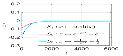
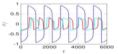
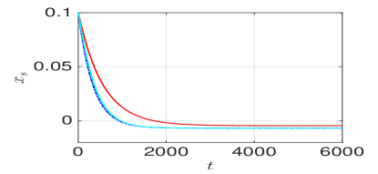
(a) $\beta-\beta_{c}<0$

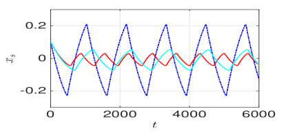
(b) $0<\beta-\beta_{c}<1$

Figure 2: States $x_{f},x_{s}$ of system (2) for different nonlinearities.

We consider several sigmoid functions, namely $S_{1}:x\mapsto\tanh(x),S_{2}:x\mapsto e^{-e^{-x}}-e^{-1},S_{3}:x\mapsto\frac{1}{1+e^{-x}}-\frac{1}{2}$. The corresponding critical values are $\beta_{c1}=1,\beta_{c2}=e$ and $\beta_{c3}=4$. We choose $\varepsilon=0.001,u=-0.01$ and $k=5$ in (8). Figure 2 illustrates the fact that, in spite of the different sigmoid nonlinearities, when $\beta-\beta_{c}<0$, the state $x_{f}$ converges to a constant value as time increases, as well as $x_{s}$, which is consistent with item 1) of Proposition 2.1. When $0<\beta-\beta_{c}<1$, both $x_{f}$ and $x_{s}$ converge to an oscillatory behavior, which is in agreement with item 2) of Proposition 2.1.

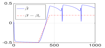
(a) without filter

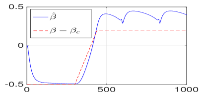
(b) with low pass filter

Figure 3: Variable $\hat{\beta}$ for two different values of $\beta$.

To check that the proposed algorithm is able to detect a change of activity of the system, we use a varying signal for $\beta$ and we consider $S=S_{1}$ and the same data as above. In particular, $\beta(t)=0.5$ on $t\in[0,300]$, it increases with slope $0.005$ on $t\in[300,425]$, and $\beta(t)=1.2$ on $t\in[425,1000]$, which leads to a change of sign of $\beta-\beta_{c}$ at $t=400$, since $\beta=\beta_{c1}=1$ in this case. We observe in Figure 3(a) that, when $\beta-\beta_{c}<0$, $\hat{\beta}$ converges to a constant value as time increases, corresponding to the resting activity. When $0<\beta-\beta_{c}<1$, $\hat{\beta}$ tends to a periodic function, which is strictly positive. Hence, it indicates the oscillation activity. The spikes seen in Figure 3(a) are due to the “jump” of the solution to system (2) from one stable branch of the critical manifold to the other. This phenomenon is captured by item 2) of Theorem 3.7, as $\hat{\beta}$ is guaranteed to be close to $\hat{\beta}^{*}$ for all time except, periodically, over interval of length $|\delta T^{\varepsilon}|=\mathcal{O}(\varepsilon)T^{\varepsilon}$. These spikes can simply be removed by using a low pass filter on $\hat{\beta}$ as illustrated in Figure 3(b). Moreover, the value of $\hat{\beta}$ evolves from negative to positive when the change of sign of $\beta-\beta_{c}$ occurs. In other words, the qualitative detector is able to detect the current activity and whether a change is occuring. We have tested different values of $k$ in (8). The simulations indicate that the speed of convergence of $\hat{\beta}$ increases with $k$. However, this also leads to bigger spikes at “jumps”, which may provide wrong information during a very short interval, which may again be moderated by a low pass filter.

The same tests have been done for $S_{2}$ and $S_{3}$. We emphasize that, even though the nonlinearities are different, the detector remains the same as defined in (8). Figure 4 shows the relationship between $\hat{\beta}$ and $\beta-\beta_{c}$ for different input $u$ and perturbation parameter $\varepsilon$. When $\beta-\beta_{c}<0$, the value of $\hat{\beta}$ provided in Figure 4 is the constant value to which it converges as seen in simulations. When $0<\beta-\beta_{c}<1$, the value of $\hat{\beta}$ reported in the figure corresponds to the average value of $\hat{\beta}$. We observe that for $\beta-\beta_{c}<0$, $\hat{\beta}$ is negative and it increases as $\beta-\beta_{c}$ increases. Moreover, because the fixed point of system (2) is near zero for small $u$, $\hat{\beta}$ evolves almost linearly with respect to $\beta-\beta_{c}$. When $0<\beta-\beta_{c}<1$, $\hat{\beta}$ is positive. In addition, when $\beta-\beta_{c}=0$, $\hat{\beta}$ is around the origin. Hence $\hat{\beta}$ is able to detect the current activity type and whether a change is likely to occur. Figure 4 illustrates the efficiency of the approach.

To further evaluate the robustness of the scheme, we have added small additive measurement noises given by $d_{out}(t)=0.005\sin(50t)$ for $x_{f},x_{s}$ and $d_{in}=0.008$ for input $u$. It is found from Figure 5 that the detector still provides good results in this case, which is in agreement with Remark 3.8.

4.2 Hodgkin-Huxley model

We consider Hodgkin-Huxley model [7]

$$C\dot{V} =\begin{aligned} &-g_{K}n^{4}(V-V_{K})\\ &-g_{Na}m^{3}h(V-V_{Na})\\ &-g_{l}(V-V_{l})+I_{app},\end{aligned}$$ (16a)

$$\tau_{m}(V)\dot{m} =-m+m_{\infty}(V),$$ (16b)

$$\tau_{n}(V)\dot{n} =-n+n_{\infty}(V),$$ (16c)

$$\tau_{h}(V)\dot{h} =-h+h_{\infty}(V),$$ (16d)

where the variable $V$ is the membrane potential. The sodium fast activation is $m$ and its slow inactivation is $h$. The potassium slow activation is $n$. The input is the applied current $I_{app}$. The parameters $V_{K},V_{Na}$ are the equilibrium potentials for the potassium and sodium ions and $V_{l}$ is the potential at which the leakage current is zero. The constant $C$ is the membrane capacity. The sodium, potassium and ionic conductances are denoted by $g_{Na},g_{K},$ and $g_{l}$. The gating variable time constants are $\tau_{m},\tau_{n},\tau_{h}$ and their steady state characteristics are $m_{\infty},n_{\infty},h_{\infty}$, which are all monotone sigmoidal functions. We consider the same parameter values as in [7] unless otherwise specified.

As explained in Remark 2.3, Hodgkin-Huxley model can be reduced to two dimensions by assuming that $m\equiv m_{\infty}(V)$ and that $h\equiv l(n)$, for a suitable linear function $l$, which is fine close to the Hopf bifurcation point via center manifold reduction [18], see e.g., [19, 20]. In its two-dimensional reduced form, Hodgkin-Huxley model falls into the class of systems (1), with $V$ the fast variable and $n$ the slow variable. The fast nullcline can also be shown to be either monotone or cubic depending on $g_{Na}$ and, since $n_{\infty}$ is monotone, the slow variable nullcline can locally be approximated as being linear. We therefore expect the detector designed for the class of system (2) to work locally for the Hodgkin-Huxley model with $u=I_{app}$ and $\beta=g_{Na}$.

In the following, we apply the proposed algorithm to the full Hodgkin-Huxley model in (16) to detect changes due to the ruling parameter $g_{Na}$. We assume that the state variables $V,n$ are measurable. The input $I_{app}$ is a constant and is assumed to be known. From (8), the detector for the Hodgkin-Huxley model is

$$\dot{\hat{g}}_{Na}=-kV(-V^{3}+\hat{g}_{Na}V+I_{app}-m),$$ (17)

where $k>0$.

In the simulations, the state variables $V,m$ are centered at zero by using a high-pass filter. We choose $k=4,I_{app}=20$. The values of $g_{Na}$ are selected from the set $\{23,25,27,29,31\}$, which gives $g_{Na}-g_{Nac}\simeq\{-4,-2,0,2,4\}$ corresponding to an approximate critical value $g_{Nac}\simeq 27$. Figure 6 shows the asymptotic value of $\hat{g}_{Na}$ as a function of $g_{Na}-g_{Nac}$, just like we did to generate Figures 4-5 in Section 4.1. The blue line corresponds to the nominal case $I_{app}=20$. Red and purple lines correspond to the perturbed cases $I_{app}=20\pm 2$. When $g_{Na}-g_{Nac}>0$, $\hat{g}_{Na}$ is selected as the average value over a period of the asymptotic periodic function to which it converges. We observe that in the nominal case, $\hat{g}_{Na}$ is negative for $g_{Na}-g_{Nac}<0$ and it increases as $g_{Na}-g_{Nac}$ increases. The value of $\hat{g}_{Na}$ is positive when $g_{Na}-g_{Nac}>0$. Moreover, $\hat{g}_{Na}$ is around zero when $g_{Na}=g_{Nac}$. Hence $\hat{g}_{Na}$ provides information about the actual activity of the model and whether the model is prone to change its activity. The perturbed cases also show that the detector performance is robust to small input uncertainties. These preliminary numerical results highlight the potentiality of the proposed approach beyond the academic example thoroughly analyzed in the present paper.

5 Conclusion

We have introduced the concept of qualitative detection, as the problem of informing on-line the qualitative dynamical behavior of a multiple-time scale nonlinear system, independently of large uncertainties on the system nonlinearities and without using any quantitative fitting of measured data. This is achieved by first extracting the system ruling parameter(s) and by subsequently designing a qualitative detector, which determines the system activity type and whether a qualitative change in the activity is close to occur. We have presented this idea on a general class of nonlinear singularly perturbed systems. As a first application, we have focused on a class of two-dimensional nonlinear systems with two time-scales and a single nonlinearity either exhibiting resting or relaxation oscillation behaviors. We have illustrated the extension of the proposed detector to real-word application through numerical simulations. Future extensions will include generalizing the detector design problem to systems exhibiting more than two possible qualitatively distinct behaviors.

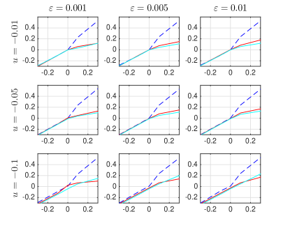
Figure 4: Evolution of $\hat{\beta}$ with $\beta-\beta_{c}$ for different sigmoid functions. Vertical axis is $\hat{\beta}$ and horizontal axis is $\beta-\beta_{c}$. Different $S$ functions: $S_{1}$ (blue dashed line), $S_{2}$ (red solid line), $S_{3}$ (light blue solid line).

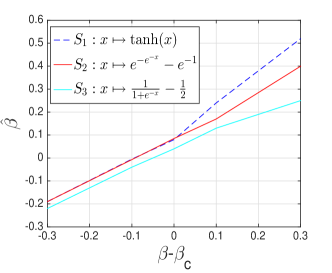
Figure 5: Evolution of $\hat{\beta}$ with $\beta-\beta_{c}$ when adding measurement noise.

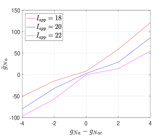
Figure 6: Evolution of the estimate $\hat{g}_{Na}$ with $g_{Na}-{g}_{Nac}$ for different input values $I_{app}$.

Appendix

Proof of Theorem 3.2. $1)$ Let $\beta\in\mathbb{R}$ and $x_{f}\in S(\mathbb{R})\setminus\{0\}$. According to (12), $\hat{\beta}^{*}(x_{f},\beta)=x^{2}_{f}-\frac{S^{-1}(x_{f})}{x_{f}}+\beta$, which is well-defined and differentiable on $S(\mathbb{R})\setminus\{0\}\times\mathbb{R}$. The only critical term for the smoothness of $\hat{\beta}^{*}$ with respect to $x_{f}$ is $\frac{S^{-1}(x_{f})}{x_{f}}$ when $x_{f}=0$. In view of items a$)$ and c$)$ of Assumption 1, the function $S^{-1}$ is differentiable. Then the Taylor expansion of $S^{-1}(x_{f})$ at the origin is, for any $x_{f}\in S(\mathbb{R})$

$$S^{-1}(x_{f})= S^{-1}(0)+(S^{-1})^{\prime}(0)x_{f}$$

$$+\frac{(S^{-1})^{\prime\prime}(0)}{2}x^{2}_{f}+\mathcal{O}(x_{f}^{3}).$$ (18)

In view of item b$)$ of Assumption 1 and (6), since $S(S^{-1}(0))=0$, it holds that $S^{-1}(0)=0$, $(S^{-1})^{\prime}(0)=\frac{1}{S^{\prime}(0)}=\beta_{c}>0$. Due to item d$)$ of Assumption 1, $(S^{-1})^{\prime\prime}(0)=-\frac{S^{\prime\prime}(0)}{(S^{\prime}(0))^{2}}=0$. We deduce from (18), $S^{-1}(x_{f})=\beta x_{f}+\mathcal{O}(x^{3}_{f})$. Then the term $\frac{S^{-1}(x_{f})}{x_{f}}$ becomes

$$\frac{S^{-1}(x_{f})}{x_{f}}=\beta_{c}+\mathcal{O}(x^{2}_{f}),$$ (19)

which is smooth with respect to $x_{f}$. This concludes the proof of the first item.
$2)$ Let $\beta\in\mathbb{R}$, we first consider that $\beta<\beta_{c}$ and $x_{f}=x_{s}\in S^{0}$. By implicitly differentiating (11) with respect to $\beta$, for $x_{f}\in S(\mathbb{R})$,

$$\frac{\partial x_{f}}{\partial\beta}=\frac{x_{f}}{-(\beta-1)+(S^{-1})^{\prime}(x_{f})}.$$ (20)

Using (12) and (20), we obtain

$$\frac{\partial\hat{\beta}^{*}(x_{f},\beta)}{\partial\beta} = \frac{\partial\hat{\beta}^{*}(x_{f},\beta)}{\partial\beta}+\frac{\partial\hat{\beta}^{*}(x_{f},\beta)}{\partial x_{f}}\frac{\partial x_{f}}{\partial\beta}$$ (21)

$$\!\!\!\!\!\!\!\!\!\!\!\!\!\!\!\!\!\!\!\!\!\!\!\!\!\!\!\!=1+\frac{\left(2x_{f}-\frac{(S^{-1})^{\prime}(x_{f})}{x_{f}}+\frac{S^{-1}(x_{f})}{x^{2}_{f}}\right)x_{f}}{-(\beta-1)+(S^{-1})^{\prime}(x_{f})}$$

$$\!\!\!\!\!\!\!\!\!\!\!\!\!\!\!\!\!\!\!\!\!\!\!\!\!\!\!\!=\frac{\left(1-\beta+2x^{2}_{f}+\frac{S^{-1}(x_{f})}{x_{f}}\right)}{-(\beta-1)+(S^{-1})^{\prime}(x_{f})}.$$

By item c$)$ of Assumption 1, $(S^{-1})^{\prime}(x_{f})=\frac{1}{S^{\prime}(S^{-1}(x_{f}))}\geqslant\frac{1}{S^{\prime}(0)}=\beta_{c}$. Since $\beta-\beta_{c}<0$, we have $-(\beta-1)+(S^{-1})^{\prime}(x_{f})\geqslant\beta_{c}-\beta+1>0$. Then the term $\frac{1}{-(\beta-1)+(S^{-1})^{\prime}(x_{f})}$ in the right-hand side of (21) is strictly positive. According to the mean value theorem, it holds $\frac{S^{-1}(x_{f})-S^{-1}(0)}{x_{f}-0}=\frac{S^{-1}(x_{f})}{x_{f}}=(S^{-1})^{\prime}(c)$ for some $c$ such that $c\in(x_{f},0)$ if $x_{f}<0$ and $c\in(0,x_{f})$ if $x_{f}>0$. Using again item c$)$ of Assumption 1, it holds $(S^{-1})^{\prime}(c)=\frac{1}{S^{\prime}(c)}\geqslant\frac{1}{S^{\prime}(0)}=\beta_{c}$. Hence, we deduce from (21) with the fact that $\beta_{c}-\beta>0$, $\frac{\partial\hat{\beta}^{*}(x_{f},\beta)}{\partial\beta}\geqslant\frac{(1+\beta_{c}-\beta+2x^{2}_{f})}{-(\beta-1)+(S^{-1})^{\prime}(x_{f})}>0$.
3$)$ Let $\beta\in(0,\beta_{c}+1)$, for any fixed $x_{s}\in\mathbb{R}$ on $S^{0}$ and $u\in\mathbb{R}$, by implicitly differentiating (11) with respect to $\beta$, we have $\frac{\partial x_{f}}{\partial\beta}=\frac{x_{f}}{-\beta+(S^{-1})^{\prime}(x_{f})}$, which is well-defined as long as $x_{f}\neq\{x^{-}_{fold},x^{+}_{fold}\}$.
We deduce from (12) and $\frac{\partial x_{f}}{\partial\beta}=\frac{x_{f}}{-\beta+(S^{-1})^{\prime}(x_{f})}$,

$$\frac{\partial\hat{\beta}^{*}(x_{f},\beta)}{\partial\beta} = \frac{\partial\hat{\beta}^{*}(x_{f},\beta)}{\partial\beta}+\frac{\partial\hat{\beta}^{*}(x_{f},\beta)}{\partial x_{f}}\frac{\partial x_{f}}{\partial\beta}$$ (22)

$$= 1+\frac{\left(2x^{2}_{f}-(S^{-1})^{\prime}(x_{f})+\frac{S^{-1}(x_{f})}{x_{f}}\right)}{-\beta+(S^{-1})^{\prime}(x_{f})}.$$

We use again $\frac{S^{-1}(x_{f})}{x_{f}}=(S^{-1})^{\prime}(c)$ for some $c$ such that $c\in(x_{f},0)$ if $x_{f}<0$ and $c\in(0,x_{f})$ if $x_{f}>0$, and write $(S^{-1})^{\prime}(c)=(S^{-1})^{\prime}(x_{f})+(S^{-1})^{\prime}(c)-(S^{-1})^{\prime}(x_{f})$. Substituting this expression into (22), we obtain

$$\frac{\partial\hat{\beta}^{*}(x_{f},\beta)}{\partial\beta}=1+\frac{(S^{-1})^{\prime}(c)-(S^{-1})^{\prime}(x_{f})+2x_{f}^{2}}{-\beta+(S^{-1})^{\prime}(x_{f})},$$ (23)

since $(S^{-1})^{\prime}(c)=\beta_{c}+\mathcal{O}(c^{2})$, $(S^{-1})^{\prime}(x_{f})=\beta_{c}+\mathcal{O}(x^{2}_{f})$ and $|c|<|x_{f}|$, it follows from (23) that $\frac{\partial\hat{\beta}^{*}(x_{f},\beta)}{\partial\beta}=1+\mathcal{O}(x_{f}^{2})$. This proves the first part of item 3$)$.

We now prove the second part of item 3$)$. Let $x_{fold}\in\{x^{+}_{fold},x^{-}_{fold}\}$. By definition of $x^{+}_{fold},x^{-}_{fold}$ in Lemma 3.2, it holds $-1+\beta S^{\prime}(S^{-1}(x_{fold}))=0,$ which is equivalent to

$$\beta=(S^{-1})^{\prime}(x_{fold}),$$ (24)

as $(S^{-1})^{\prime}(x_{fold})=\frac{1}{S^{\prime}(S^{-1}(x_{fold}))}$.

We deduce from (22) by using (24),

$$\frac{\partial\hat{\beta}^{*}(x_{f},\beta)}{\partial\beta} = 1+\frac{\left(2x^{2}_{f}-(S^{-1})^{\prime}(x_{f})+\frac{S^{-1}(x_{f})}{x_{f}}\right)}{-\beta+(S^{-1})^{\prime}(x_{f})}$$ (25)

$$= \frac{\left(-\beta+2x^{2}_{f}+\frac{S^{-1}(x_{f})}{x_{f}}\right)}{-\beta+(S^{-1})^{\prime}(x_{f})}$$

$$= \frac{\left(-(S^{-1})^{\prime}(x_{fold})+2x^{2}_{f}+\frac{S^{-1}(x_{f})}{x_{f}}\right)}{-\beta+(S^{-1})^{\prime}(x_{f})}.$$

By virtue of items c$)$ and d$)$ of Assumption 1, the following holds, for $x_{f}\in(-\infty,x^{-}_{fold})\cup(x^{+}_{fold},+\infty)$

$$-1+\beta S^{\prime}(S^{-1}(x_{f}))<0.$$ (26)

Dividing both sides of the above inequality by $S^{\prime}(S^{-1}(x_{f}))$, which is strictly positive, and using $(S^{-1})^{\prime}(x_{f})=\frac{1}{S^{\prime}(S^{-1}(x_{f}))}$, we obtain

$$-\beta+(S^{-1})^{\prime}(x_{f}) >0.$$ (27)

This implies that the denominator of (25) is strictly positive. We denote $g(x_{f})=\frac{(S^{-1})(x_{f})}{x_{f}}$. The derivative of $g(x_{f})$ is given by

$$g^{\prime}(x_{f}) =\frac{x_{f}(S^{-1})^{\prime}(x_{f})-S^{-1}(x_{f})}{x^{2}_{f}}.$$ (28)

We show below that the growth of $g(x_{f})$ increases with $|x_{f}|$. According to item c$)$ of Assumption 1, it holds $(S^{-1})^{\prime}(x_{f})=\frac{1}{S^{\prime}(S^{-1}(x_{f}))}>0$. Hence, the function $S^{-1}$ is strictly increasing. Moreover, item b$)$ of Assumption 1 implies $S^{-1}(0)=0$. We first consider the case where $x_{f}>0$. It holds that $S^{-1}(x_{f})>0$ for all $x_{f}>0$. Using $\frac{(S^{-1})(x_{f})}{x_{f}}=(S^{-1})^{\prime}(c)$ as previously done in this proof, for some $c$ such that $c\in(0,x_{f})$ and in view of items c$)$ and d$)$ of Assumption 1, $S^{\prime}(S^{-1}(x_{f}))<S^{\prime}(S^{-1}(c))$ for $x_{f}>c>0$, and thus $(S^{-1})^{\prime}(x_{f})=\frac{1}{S^{\prime}(S^{-1}(x_{f}))}>\frac{1}{S^{\prime}(S^{-1}(c))}=(S^{-1})^{\prime}(c)$. It holds that $\frac{(S^{-1})(x_{f})}{x_{f}}=(S^{-1})^{\prime}(c)<(S^{-1})^{\prime}(x_{f})$. Then, we deduce

$$x_{f}(S^{-1})^{\prime}(x_{f})-(S^{-1})(x_{f})>0.$$ (29)

In view of (28) and (29), we have $g^{\prime}(x_{f})>0$ for all $x_{f}>0$, which means that $\frac{S^{-1}(x_{f})}{x_{f}}$ increases with $x_{f}$ when $x_{f}>0$. Similar arguments show that $\frac{S^{-1}(x_{f})}{x_{f}}$ increases with $|x_{f}|$ when $x_{f}<0$. Therefore, the term $\frac{S^{-1}(x_{f})}{x_{f}}$, as well as $2x^{2}_{f}$, increases when $x_{f}\in(-\infty,x^{-}_{fold})\cup(x^{+}_{fold},+\infty)$. Under condition (13), $-(S^{-1})^{\prime}(x_{fold})+2x^{2}_{f}+\frac{S^{-1}(x_{f})}{x_{f}}$ is strictly positive for $x_{f}\in(-\infty,x^{-}_{fold})\cup(x^{+}_{fold},+\infty)$. Recall that $\frac{1}{-\beta+(S^{-1})^{\prime}(x_{f})}$ in (25) is strictly positive, we obtain the desired result.

4$)$ Combining (12) and (19), we obtain for any $x_{f}\in S(\mathbb{R})$ and $\beta\in\mathbb{R}$, $\hat{\beta}^{*}(x_{f},\beta)=\beta-\beta_{c}+\mathcal{O}(x^{2}_{f})$.
This concludes the proof of the last item. $\hfill\blacksquare$

Proof of Proposition 3.4. Two steps are used to prove this proposition. We first show a boundedness property for system (8). Then we prove that (14) holds. Let $\Delta,M,T,\mu>0$ and $x_{f},x_{s},u$ be such that conditions $(i)$ and $(ii)$ of Proposition 3.4 hold. We rewrite (8) as follows

$$\dot{\hat{\beta}}=-kx^{2}_{f}\hat{\beta}+\biggl{(}kx^{4}_{f}+kx_{f}(x_{s}-u)\biggr{)}.$$ (30)

System (30) can be interpreted as a linear time-varying system with input $kx^{4}_{f}+kx_{f}(x_{s}-u)$. We first consider the following nominal system

$$\dot{\hat{\beta}}=-kx^{2}_{f}\hat{\beta}.$$ (31)

Solutions to system (31) are given for $t\geqslant 0$ by $\hat{\beta}(t)=\Phi(t,0)\hat{\beta}(0)$, where $\Phi(t,s):=\exp\left(\int_{s}^{t}-kx^{2}_{f}(\tau)\;d\tau\right)$ and $|\Phi(t,0)|\leqslant 1$ for all $t\geqslant 0$. Hence the origin is stable for system (31).
Let $|\hat{\beta}(0)|\leqslant\Delta$ and consider the following Lyapunov function candidate for system (30)

$$V(t,\hat{\beta}):=p(t)\hat{\beta}^{2},$$ (32)

where $p(t)\!\!:=\!\!\int_{t}^{\infty}\Phi^{2}(s,t)\;\!\!ds$. We show below that $V(t,\hat{\beta})$ is positive definite and radially unbounded with respect to $\hat{\beta}$, uniformly in $t$. For $0\leqslant t\leqslant s$, we write

$$p(t)=\int_{t}^{\infty}\Phi^{2}(s,t)\;ds=\int_{t}^{\infty}\exp\left(\int_{t}^{s}-2kx^{2}_{f}(\tau)\;d\tau\right)ds.$$ (33)

Since $x_{f}$ is $(T,\mu)$-PE by assumption, for $t\leqslant s<t+T$, $\mu\leqslant\int_{t}^{t+T}x^{2}_{f}(\tau)d\tau=\int_{t}^{s}x^{2}_{f}(\tau)d\tau+\int_{s}^{t+T}x^{2}_{f}(\tau)d\tau$. Hence,

$$\int_{t}^{s}x^{2}_{f}(\tau)d\tau \geqslant \mu-\int_{s}^{t+T}x^{2}_{f}(\tau)d\tau.$$ (34)

Under assumption $\max(\|x_{f}\|_{\infty},\|x_{s}\|_{\infty},\|u\|_{\infty})\leqslant M$, we deduce from (33) and (34)

$$p(t) = \int_{t}^{\infty}\exp\left(\int_{t}^{s}-2kx^{2}_{f}(\tau)\;d\tau\right)ds$$ (35)

$$\leqslant \int_{t}^{\infty}\exp\left(-2k\mu+2k\int^{t+T}_{s}x^{2}_{f}(\tau)\;d\tau\right)ds$$

$$\leqslant \exp(-2k\mu)\int_{t}^{\infty}\exp\left(2kM^{2}(t+T-s)\right)ds$$

$$\leqslant \frac{\exp(2kM^{2}T)}{2kM^{2}}.$$

We also have from (33)

$$p(t) =\int_{t}^{\infty}\exp\left(\int_{t}^{s}-2kx^{2}_{f}(\tau)\;d\tau\right)ds$$

$$\geqslant\int_{t}^{\infty}\exp\left(-2kM^{2}(s-t)\right)ds\geqslant\frac{1}{2kM^{2}}.$$ (36)

Hence, $V(t,\hat{\beta})$ is lower and upper bounded as

$$\frac{1}{2kM^{2}}|\hat{\beta}|^{2}\leqslant V(t,\hat{\beta})\leqslant\frac{\exp(2kM^{2}T)}{2kM^{2}}|\hat{\beta}|^{2}.$$ (37)

The time-derivative of $V(t,\hat{\beta})$ along the solution to (30) is, for any $t\geqslant 0$,

$$\frac{\partial V}{\partial t}+\frac{\partial V}{\partial\hat{\beta}}\hat{f}(\hat{\beta},x_{f},u-x_{s})$$

$$= \dot{p}(t)\hat{\beta}^{2}+2p(t)\hat{\beta}\left(-kx^{2}_{f}\hat{\beta}+\left(kx^{4}_{f}+kx_{f}(x_{s}-u)\right)\right)$$

$$= \left(\dot{p}(t)-2kx^{2}_{f}p(t)\right)\hat{\beta}^{2}+2\hat{\beta}p(t)\left(kx^{4}_{f}+kx_{f}(x_{s}-u)\right).$$

Since $\Phi(t,t)=1$ and $\frac{d\Phi(s,t)}{dt}=\Phi(s,t)kx^{2}_{f}$, we deduce after some calculations that

$$\dot{p}(t)-2kx^{2}_{f}p(t)=-1.$$ (39)

Using (35) and (39), $\frac{\partial V}{\partial t}+\frac{\partial V}{\partial\hat{\beta}}\hat{f}(\hat{\beta},x_{f},u-x_{s})\leqslant-|\hat{\beta}|^{2}+2|\hat{\beta}|\frac{\exp(2kM^{2}T)\widetilde{C}(M)}{2kM^{2}}$. According to [24, Theorem 4.18], we conclude the boundedness property of (8) from (37) and $\frac{\partial V}{\partial t}+\frac{\partial V}{\partial\hat{\beta}}\hat{f}(\hat{\beta},x_{f},u-x_{s})\leqslant-|\hat{\beta}|^{2}+2|\hat{\beta}|\frac{\exp(2kM^{2}T)\widetilde{C}(M)}{2kM^{2}}$. That is, there exists $\bar{\eta}(\Delta,M,T)>0$ such that solution $\hat{\beta}$ to system (30) holds $|\hat{\beta}(t)|\leqslant\bar{\eta}(\Delta,M,T)$, for all $t\geqslant 0$.
To prove (14), let $x_{f},x_{s},u$ be such that conditions $(i)$ and $(ii)$ of Proposition 3.4 holds, we define for $t\geqslant 0$,

$$W(t,\hat{\beta}_{1},\hat{\beta}_{2}):=p_{1}(t)(\hat{\beta}_{1}-\hat{\beta}_{2})^{2},$$ (40)

where $p_{1}(t):=\int_{t}^{\infty}\Phi_{1}^{2}(s,t)\;ds$, and $\Phi_{1}(t,0):=\exp\left(\int_{0}^{t}-kx^{2}_{f1}(\tau)d\tau\right)$. For $|\hat{\beta}_{1}(0)|,|\hat{\beta}_{2}(0)|\leqslant\Delta$, similar computations in (35)-(36) shows, for any $t\geqslant 0$

$$\frac{1}{2kM^{2}}|\hat{\beta}_{1}-\hat{\beta}_{2}|^{2} \leqslant W(t,\hat{\beta}_{1},\hat{\beta}_{2})$$ (41)

$$\leqslant \frac{\exp(2kM^{2}T)}{2kM^{2}}|\hat{\beta}_{1}-\hat{\beta}_{2}|^{2}.$$

Following the similar computations for (39), we obtain $\dot{p}_{1}(t)-2kx^{2}_{f1}p_{1}(t)=-1$. The following holds along to the solutions to (30) for any $t\geqslant 0$, where the time arguments are omitted,

$$\!\!\!\!\!\!\!\!\frac{\partial W}{\partial t}+\frac{\partial W}{\partial\hat{\beta}_{1}}\hat{f}(\hat{\beta}_{1},x_{f1},u_{1}-x_{s1})+\frac{\partial W}{\partial\hat{\beta}_{2}}\hat{f}(\hat{\beta}_{2},x_{f2},u_{2}-x_{s2})$$ (42)

$$\!\!\!\!= \!\!\!\dot{p}_{1}(t)(\hat{\beta}_{1}-\hat{\beta}_{2})^{2}+2p_{1}(t)(\hat{\beta}_{1}-\hat{\beta}_{2})\biggl{(}-kx^{2}_{f1}\hat{\beta}_{1}+\left(kx_{f1}^{4}\right.$$

$$\!\!\!\!\!\!\!\!\left.+kx_{f1}(x_{s1}-u_{1})\right)+kx^{2}_{f2}\hat{\beta}_{2}-\left(kx_{f2}^{4}+kx_{f2}(x_{s2}-u_{2})\right)\biggr{)}$$

$$= \left(\dot{p}_{1}(t)-2kx^{2}_{f1}p_{1}(t)\right)(\hat{\beta}_{1}-\hat{\beta}_{2})^{2}+2kp_{1}(t)(\hat{\beta}_{1}-\hat{\beta}_{2})$$

$$\!\!\!\!\times\biggl{(}-\hat{\beta}_{2}(x^{2}_{f1}-x^{2}_{f2})+(x^{4}_{f1}-x^{4}_{f2})+x_{s2}(x_{f1}-x_{f2})$$

$$\!\!\!\!+x_{f1}(x_{s1}-x_{s2})-x_{f1}(u_{1}-u_{2})-u_{2}(x_{f1}-x_{f2})\biggr{)}.$$

Under condition $(ii)$, $\dot{p}_{1}(t)-2kx^{2}_{f1}p_{1}(t)=-1$, and the fact that $x\mapsto x^{4}$ and $x\mapsto x^{2}$ are locally Lipschitz, we derive that there exists $\rho(\Delta,M,T)>0$ such that $\frac{\partial W}{\partial t}+\frac{\partial W}{\partial\hat{\beta}_{1}}\hat{f}(\hat{\beta}_{1},x_{f1},u_{1}-x_{s1})+\frac{\partial W}{\partial\hat{\beta}_{2}}\hat{f}(\hat{\beta}_{2},x_{f2},u_{2}-x_{s2})\leqslant-|\hat{\beta}_{1}-\hat{\beta}_{2}|^{2}+\rho(\Delta,M,T)|\hat{\beta}_{1}-\hat{\beta}_{2}|(|x_{f1}-x_{f2}|+|x_{s1}-x_{s2}|+|u_{1}-u_{2}|)$, we then obtain the desired result by following the similar analysis as in the first step of this proof. $\hfill\blacksquare$

Proof of Lemma 3.5. We first prove item 1). Let $\Delta>\delta>0$. For any $\beta-\beta_{c}<0$, any constant input $\delta<|u|<\Delta$, according to item 1 of Proposition 2.1, there exists $\bar{\varepsilon}$ such that for any $\varepsilon\in(0,\bar{\varepsilon}]$ and any $|x_{f}(0)|,|x_{s}(0)|\leqslant\Delta$, it holds $|(x_{f}(t)-x_{f}^{*}),(x_{s}(t)-x_{s}^{*})|\leqslant c(\Delta,\delta)e^{-\sigma(\Delta,\delta)t}|(x_{f}(0)-x^{*}_{f}),(x_{s}(0)-x^{*}_{s})|$, for $t\geqslant 0$, where the fixed point $(x^{*}_{f},x^{*}_{s})$ is different from $(0,0)$ (because $u\neq 0$) and $c(\Delta,\delta),\sigma(\Delta,\delta)>0$. Hence, condition $(ii)$ of item 1) of Lemma 3.5 holds. We also deduce that there exists $T_{1}(\Delta,\delta)>0$ such that $|x_{f}(t)-x_{f}^{*}|\leqslant\frac{|x_{f}^{*}|}{2}$ for any $t\geqslant T_{1}(\Delta,\delta)$. It holds that for $t\geqslant T_{1}(\Delta,\delta)$, $|x_{f}(t)|=|x_{f}(t)-x^{*}_{f}+x^{*}_{f}|\geqslant|x^{*}_{f}|-|x_{f}(t)-x^{*}_{f}|\geqslant|x^{*}_{f}|-\frac{|x^{*}_{f}|}{2}=\frac{|x^{*}_{f}|}{2}$. Let $T(\Delta,\delta)>T_{1}(\Delta,\delta)$, we deduce, for any $t\geqslant 0$

$$\int_{t}^{t+T(\Delta,\delta)}\!\!\!\!x^{2}_{f}(\tau)d\tau=\!\!\int_{t}^{t+T_{1}(\Delta,\delta)}\!\!\!\!\!\!x^{2}_{f}(\tau)d\tau+\!\!\int_{t+T_{1}(\Delta,\delta)}^{t+T(\Delta,\delta)}\!\!\!\!\!\!x^{2}_{f}(\tau)d\tau$$

$$\geqslant\int_{t+T_{1}(\Delta,\delta)}^{t+T(\Delta,\delta)}|x_{f}(\tau)|^{2}d\tau\geqslant\left(\frac{|x^{*}_{f}|}{2}\right)^{2}\!\!\!\!(T(\Delta,\delta)-T_{1}(\Delta,\delta)).$$

Thus, condition $(i)$ of item 1) of Lemma 3.5 holds with $\mu(\Delta,\delta)=\left(\frac{|x^{*}_{f}|}{2}\right)^{2}\times(T(\Delta,\delta)-T_{1}(\Delta,\delta))$.

We next prove item 2). Let $\Delta>\delta>0$, for any $0<\beta-\beta_{c}<1$ and for any input $u\in(-\bar{u},\bar{u})$, where $\bar{u}\in(0,\Delta]$, according to item 2) of Proposition 2.1, there exists $\bar{\varepsilon}$ such that for all $\varepsilon\in(0,\bar{\varepsilon}]$, and $|x_{f}(0)|,|x_{s}(0)|\leqslant\Delta$ and $|x_{f}(0)-p^{*}_{f}|,|x_{s}(0)-p^{*}_{s}|\geqslant\delta$, all trajectories of system (2) converge to an asymptotic periodic orbit $P^{\varepsilon}$ with period $T^{\varepsilon}$ and it is locally exponentially stable. Thus solutions $x_{f},x_{s}$ to system (2) are bounded. Therefore, condition $(ii)$ of item 2) of Lemma 3.5 holds. Moreover, let $|x_{f}^{lc}|$ be the absolute value of $x_{f}$-component of $P^{\varepsilon}$, which is $T^{\varepsilon}$-periodic. The average value of $|x^{lc}_{f}|$ over a period is denoted by $\bar{x}_{f}=\frac{1}{T^{\varepsilon}}\int_{t}^{t+T^{\varepsilon}}|x^{lc}_{f}(\tau)|d\tau$ for all $t\geqslant 0$ and it is strictly positive. Due to the globally attractivity of $P^{\varepsilon}$, for any $\eta>0$ there exists $T_{1}(\Delta,\delta,\eta)>0$ such that $|x_{f}(t)-\bar{x}_{f}|\leqslant\eta$ for $t\geqslant T_{1}(\Delta,\delta,\eta)$. Let $T(\Delta,\delta)=T_{1}(\Delta,\delta,\eta)+T^{\varepsilon}$, the following holds

$$\int_{t}^{t+T(\Delta,\delta)}\!\!\!\!\!\!x^{2}_{f}(\tau)d\tau\!\!=\!\!\!\!\int_{t}^{t+T_{1}(\Delta,\delta,\eta)}\!\!\!\!\!\!\!\!x^{2}_{f}(\tau)d\tau+\!\!\int_{t+T_{1}(\Delta,\delta,\eta)}^{t+T(\Delta,\delta)}\!\!\!\!\!\!x^{2}_{f}(\tau)d\tau$$

$$\geqslant\int_{t+T_{1}(\Delta,\delta)}^{t+T(\Delta,\delta)}\bar{x}^{2}_{f}d\tau+\int_{t+T_{1}(\Delta,\delta)}^{t+T(\Delta,\delta)}(x^{2}_{f}(\tau)-\bar{x}^{2}_{f})d\tau$$

$$\geqslant\bar{x}^{2}_{f}T^{\varepsilon}-\int_{t+T_{1}(\Delta,\delta)}^{t+T(\Delta,\delta)}|x^{2}_{f}(\tau)-\bar{x}^{2}_{f}|d\tau.$$ (43)

Since $x\mapsto x^{2}$ is locally Lipschitz, it holds $|x^{2}_{f}(t)-\bar{x}^{2}_{f}|\leqslant\psi(\Delta,\delta)|x_{f}(t)-\bar{x}_{f}|$. We deduce from (43)

$$\int_{t}^{t+T(\Delta,\delta)}x^{2}_{f}(\tau)d\tau \geqslant \bar{x}^{2}_{f}T^{\varepsilon}-\int_{t+T_{1}(\Delta,\delta)}^{t+T(\Delta,\delta)}|x^{2}_{f}(\tau)-\bar{x}^{2}_{f}|d\tau$$ (44)

$$\geqslant\bar{x}^{2}_{f}T^{\varepsilon}-\psi(\Delta,\delta)\eta T^{\varepsilon}.$$

Let choose $T_{1}(\Delta,\delta,\eta)$ sufficiently large such that $\eta=\frac{\bar{x}_{f}}{2\psi(\Delta,\delta)}$. Then, the above inequality follows

$$\int_{t}^{t+T(\Delta,\delta)}x^{2}_{f}(\tau)d\tau \geqslant\bar{x}^{2}_{f}T^{\varepsilon}-\psi(\Delta,\delta)\eta T^{\varepsilon}=\frac{\bar{x}^{2}_{f}}{2}T^{\varepsilon}.$$

Thus, condition $(i)$ of item 2) of Lemma 3.5 holds with $\mu(\Delta,\delta)=\frac{\bar{x}^{2}_{f}}{2}T^{\varepsilon}$. $\hfill\blacksquare$

Proof of Theorem 3.6. In the following, we denote the $(x_{f},x_{s})$-component of the solutions to (15) as $x$. We first prove item 1). Let $\Delta>\delta>0$, $\beta<\beta_{c}$ and constant input $\delta<|u|<\Delta$, according to item 1) of Proposition 1, there exists $\bar{\varepsilon}>0$ such that for any $\varepsilon\in(0,\bar{\varepsilon}]$ and any $|x(0)|\leqslant\Delta$, the corresponding solution $x$ to subsystem (15a)-(15b) satisfies for $t\geqslant 0$,

$$|x(t)-x^{*}|\leqslant c_{1}(\Delta,\delta)e^{-c_{2}(\Delta,\delta)t}|x(0)-x^{*}|,$$ (45)

where $x^{*}:=(x^{*}_{f},x^{*}_{s})$ is the fixed point of subsystem (15a)-(15b), and $c_{1}(\Delta,\delta),c_{2}(\Delta,\delta)>0$.

We next consider for $t\geqslant 0$,

$$W(t,\hat{\beta}):=p(t)(\hat{\beta}-\bar{\hat{\beta}})^{2},$$ (46)

where $\bar{\hat{\beta}}$ is the equilibrium point of (15c) associated with constant input $(x^{*},u)$, and $p(t)\!\!:=\!\!\int_{t}^{\infty}\Phi^{2}(s,t)\;ds$ as in the proof of Proposition 3.4. For any $|\hat{\beta}(0)|\leqslant\Delta$, by the similar computations in (35)-(36) for any $t\geqslant 0$

$$\underline{M}(\Delta,\delta)|\hat{\beta}-\bar{\hat{\beta}}|^{2} \leqslant W(t,\hat{\beta})\leqslant\overline{M}(\Delta,\delta)|\hat{\beta}-\bar{\hat{\beta}}|^{2},$$ (47)

where $\underline{M}(\Delta,\delta),\overline{M}(\Delta,\delta)>0$. Following similar lines as in (39), we obtain $\dot{p}(t)-2kx^{2}_{f}p(t)=-1$, and we derive that for any $t\geqslant 0$, where the time arguments are omitted,

$$\frac{\partial W}{\partial t}+\frac{\partial W}{\partial\hat{\beta}}\hat{f}(\hat{\beta},x_{f},u-x_{s})$$

$$\leqslant -|\hat{\beta}-\bar{\hat{\beta}}|^{2}+\nu(\Delta,\delta)|\hat{\beta}-\bar{\hat{\beta}}|\left(|x_{f}-x^{*}_{f}|+|x_{s}-x^{*}_{s}|\right),$$

where $\nu(\Delta,\delta)>0$. We deduce from the above inequality

$$|\beta(t)-\bar{\hat{\beta}}|^{2} \leqslant c_{3}(\Delta,\delta)e^{-c_{4}(\Delta,\delta)t}|\hat{\beta}(0)-\bar{\hat{\beta}}|^{2}$$ (49)

$$+c_{5}(\Delta,\delta)e^{-c_{4}(\Delta,\delta)t}|x(0)-x^{*}|^{2},$$

with $c_{3}(\Delta,\delta),c_{4}(\Delta,\delta),c_{5}(\Delta,\delta)>0$. This property together with (45) imply that the semiglobal exponential stability of system (15), which, in turn, implies the global asymptotic stability, according to [21, Proposition 3.4]. Thus, the desired result follows.

We next prove item 2). Let $\Delta>0$. For any $0<\beta-\beta_{c}<1$, according to item 2) of Proposition 1, there exist $\bar{\varepsilon}>0,\bar{u}\in(0,\Delta)$ such that for any $\varepsilon\in(0,\bar{\varepsilon}]$, for any $u\in(-\bar{u},\bar{u})$, there exists $m>0$ such that for any $|x(0)|_{P^{\varepsilon}}\leqslant m$ except the unique unstable fixed point of (15a)-(15b), the corresponding solution $x$ to subsystem (15a)-(15b) satisfies for $t\geqslant 0$,

$$|x(t)|_{P^{\varepsilon}}\leqslant c_{6}(m)e^{-c_{7}(m)t}|x(0)|_{P^{\varepsilon}},$$ (50)

where $P^{\varepsilon}$ is the periodic solution of subsystem (15a)-(15b) and $c_{6}(m),c_{7}(m)>0$. By virtue of Lemma 2 and Proposition 2, subsystem (15c) is semiglobally incrementally ISS. Then according to [21, Proposition 4.4], there exists initial condition $\bar{\hat{\beta}}^{lc}(0)$ such that $\bar{\hat{\beta}}^{lc}(t)$ is a periodic solution to (15c) with periodic input $(P^{\varepsilon},u)$. We choose $W(t,\hat{\beta}):=p(t)(\hat{\beta}-\bar{\hat{\beta}}^{lc})^{2}$. Then using similar arguments as above we obtain the local exponential stability of system (15) with respect to a limit cycle.

Due to [21, Proposition 4.5], for any initial condition $x(0)$ except the unique unstable fixed point $x^{*}$ of subsystem (15a)-(15b), the corresponding solution to system (15c) holds $\lim\limits_{t\to\infty}|\hat{\beta}(t)|_{\bar{\hat{\beta}}^{lc}}=0$ as $\lim\limits_{t\to\infty}|x(t)|_{P^{\varepsilon}}=0$ . In addition, local exponential stability implies local stability, then the desired result follows.

Proof of Theorem 3.7. We start by proving item 1). By Theorem 3.6, if $\beta<\beta_{c}$ then $(x_{f}(t),x_{s}(t))\to(x^{*}_{f},x^{*}_{s})$ and $\hat{\beta}(t)\to\bar{\hat{\beta}}$ as time goes to infinity. Note that, since $(x^{*}_{f},x^{*}_{s})$ is a steady-state of (15a)-(15b), it must satisfies $(x^{*}_{f},x^{*}_{s})\in S^{0}$. Moreover, $u\neq 0$ implies $x^{*}_{f}\neq 0$. Because $-kx^{*}_{f}(-x^{*3}_{f}+\bar{\hat{\beta}}x^{*}_{f}+u-x^{*}_{s})=0$ and $(x^{*}_{f},x^{*}_{s})\in S^{0}$, it follows that $\bar{\hat{\beta}}=\frac{x^{*3}_{f}-S^{-1}(x^{*}_{f})+\beta x^{*}_{f}}{x^{*}_{f}}=\hat{\beta}^{*}(x^{*}_{f},\beta)$.

We next prove item 2). At the singular limit $\epsilon=0$, the one dimensional estimate critical manifold $R^{0}$ of system (15) is defined by the following two equations

$$[left=\empheqlbrace\,]0 =-x_{f}+S(\beta x_{f}+u-x_{s}),$$

$$0 =-x_{f}^{3}+\hat{\beta}x_{f}+u-x_{s},$$

which can explicitly be solved as rCl R^0&={(x_f,x_s,^β):
x_s=ϕ(x_f,u,β):=-S^-1(x_f)+βx_f+u,
^β= xf3-u+ϕ(xf,u,β)xf=^β^*(x_f,β)}. Note that the $(x_{f},x_{s})$-projection of $R^{0}$ is $S^{0}$.
The layer dynamics reads

$$[left=\!\!\!\!\empheqlbrace\,]\dot{x}_{f} =-x_{f}+S(\beta x_{f}+u-x_{s}),\IEEEyessubnumber$$ (52a)

$$\dot{x}_{s} =0,\IEEEyessubnumber$$ (52b)

$$\dot{\hat{\beta}} =-kx_{f}(-x_{f}^{3}+\hat{\beta}x_{f}+u-x_{s}).\IEEEyessubnumber$$ (52c)

To study the normal hyperbolicity of $R^{0}$, we compute the Jacobian matrix of (52) on $R^{0}$ as

$$\!\!\!\!J \!\!=\!\! \begin{pmatrix}\!\!\!\!\!\!-1+\beta S^{\prime}(\beta x_{f}+u-x_{s})&\!\!\!\!-S^{\prime}(\beta x_{f}+u-x_{s})&0\\ 0&0&0\\ 4kx_{f}^{3}-2k\hat{\beta}x_{f}-k(u-x_{s})&kx_{f}&-kx_{f}^{2}\end{pmatrix}$$

for $x_{s}=\phi(x_{f},u,\beta)$, $\hat{\beta}=\hat{\beta}^{*}(x_{f},\beta)$. The two nonzero eigenvalues are $\lambda_{1}=-kx^{2}_{f},\;\lambda_{2}=-1+\beta S^{\prime}(S^{-1}(x_{f}))$. For $0<\beta-\beta_{c}<1$, it holds that $\beta>\beta_{c}=\frac{1}{S^{\prime}(0)}$, which is equivalent to $\frac{1}{\beta}<S^{\prime}(0)$ and therefore, invoking item d) of Assumption 1, the equation $-1+\beta S^{\prime}(S^{-1}(x_{f}))=0$ has exactly one positive and negative roots, $x_{fold}^{+}$ and $x_{fold}^{-}$, respectively. Moreover,

$$\lambda_{2}\left\{\begin{array}[]{rl}<0,&{\rm if}\ x_{f}<x_{fold}^{-}\ {\rm or}\ x_{f}>x_{fold}^{+},\\ >0,&{\rm if}\ x_{fold}^{-}<x_{f}<x_{fold}^{+}.\end{array}\right.$$

Since $\lambda_{1}<0$ for $x_{f}\neq 0$, it follows that two branches of $R^{0}$ given by rCl R^0_+&:=R^0∩{x_f¿x_fold^+},
R^0_-:=R^0∩{x_f¡x_fold^-}, are locally exponentially attractive branches of the estimate critical manifold $R^{0}$. Let

$$\hat{\beta}_{fold}^{+}=\hat{\beta}^{*}(x_{fold}^{+},\beta),\;\hat{\beta}_{fold}^{-}=\hat{\beta}^{*}(x_{fold}^{-},\beta),$$

$$x_{s,fold}^{+}=\phi(x_{fold}^{+},u,\beta),\;x_{s,fold}^{-}=\phi(x_{fold}^{-},u,\beta).$$

The end points of $R^{0}_{+}$ and $R^{0}_{-}$ are given by

$$F^{+}:=(x_{fold}^{+},\hat{\beta}_{fold}^{+},x_{s,fold}^{+}),\;F^{-}:=(x_{fold}^{-},\hat{\beta}_{fold}^{-},x_{s,fold}^{-})$$

respectively, are fold points of the estimate critical manifold $R^{0}$. See Figure 7.

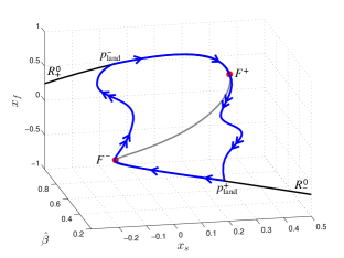
Figure 7:

The slow flow on $R^{0}$ is defined by the reduced dynamics

$$[left=\empheqlbrace\,]0 =-x_{f}+S(\beta x_{f}+u-x_{s}),\IEEEyessubnumber$$ (53a)

$$x_{s}^{\prime} =x_{f}-x_{s},\IEEEyessubnumber$$ (53b)

$$0 =-kx_{f}(-x_{f}^{3}+\hat{\beta}x_{f}+u-x_{s}).\IEEEyessubnumber$$ (53c)

The flow on $R^{0}_{+}$, as well as on $R^{0}_{-}$, with respect to the reduced dynamics of (53) is given as follows. It holds that $x_{s}^{\prime}<0(x_{f}<x_{s}<0)$ on $R^{0}_{-}$ and, similarly, $x_{s}^{\prime}>0$ on $R^{0}_{+}$. Noticing that the $x_{s}$-projection of $R^{0}_{+}$ (resp. $R^{0}_{-}$) is the semiline $(-\infty,x^{+}_{s,fold})$ (resp. $(x^{-}_{s,fold},\infty)$), it follows that all trajectories on $R^{0}_{+}$ eventually reach the fold point $F^{+}$. Conversely, all trajectories on $R^{0}_{-}$ eventually reach $F^{-}$ (see Fig. 7).

At the folds, we connect the slow flow with the (two-dimensional) fast flow. We claim that the fast flow brings the trajectory on the opposite branch of the critical manifold. Indeed, by monotonicity of (52a), $x_{f}$ converges to equilibrium. By the cascade structure of (52a)-(52c) and incremental ISS property of (52c), $\hat{\beta}$ also converges to equilibrium. Because the only equilibria of (52a)-(52c) are on the estimate critical manifold, the result follows.

We have therefore constructed a candidate singular periodic orbit $Q^{0}$. The persistence of this singular orbit for $\varepsilon>0$ follows as in the proof of Proposition 2.1 and is omitted. Let $Q^{\varepsilon}$ be the resulting periodic orbit of (15). By Theorem 3.6, almost all the trajectories of system (15) asymptotically converge to $Q^{\varepsilon}$. Following again the same arguments as the proof of Proposition 2.1, it holds that trajectories along $Q^{\varepsilon}$ spend only an $\mathcal{O}(\varepsilon)$-fraction of the limit cycle period outside an $\mathcal{O}(\varepsilon)$ neighborhood of the estimate critical manifold. Because $\hat{\beta}(t)=\hat{\beta}^{*}(x^{lc}_{f}(t+\theta),\beta)$ on the estimate critical manifold, the result follows.$\hfill\blacksquare$

References

• [1] Y. Tang, A. Franci, and R. Postoyan. Qualitative parameter estimation for a class of relaxation oscillators. In 20th IFAC World Congress, Toulouse, France, 2017.
• [2] M.S. Goldman, J. Golowasch, E. Marder, and L.F. Abbott. Global structure, robustness, and modulation of neuronal models. J. Neurosci., 21(14):5229–5238, 2001.
• [3] E. Marder. Variability, compensation, and modulation in neurons and circuits. PNAS, 108:15542–15548, 2011.
• [4] G. Drion, A. Franci, J. Dethier, and R. Sepulchre. Dynamic input conductances shape neuronal spiking. eNeuro, 2(1):e0031–14.2015: 1–15, 2015.
• [5] A. Franci, G. Drion, and R. Sepulchre. Modeling the modulation of neuronal bursting: a singularity theory appraoch. SIAM J. Appl. Dyn. Syst., 13(2):798–829, 2014.
• [6] G. Drion, T. O’Leary, J. Dethier, A. Franci, and R. Sepulchre. Neuronal behaviors: a control perspective. In IEEE Conference on Decision and Control, pages 1923–1944, Osaka, Japan, 2015. Tutorial paper.
• [7] A. Hodgkin and A. Huxley. A quantitative description of membrane current and its application to conduction and excitation in nerve. J. Physiol., 117:500–544, 1952.
• [8] H.R. Wilson and J.D. Cowan. Excitatory and inhibitory interactions in localized populations of model neurons. Biophys J, 12(1):1–24, 1972.
• [9] M. Golubitsky and D.G. Schaeffer. Singularities and Groups in Bifurcation Theory. Springer, 1985.
• [10] A. Franci and R. Sepulchre. Realization of nonlinear behaviors from organizing centers. In IEEE Conference on Decision and Control, pages 56–61, Los Angeles, California, USA, 2014.
• [11] L. Moreau and E. Sontag. Balancing at the border of instability. Physical Review, 68:020901:1–4, 2003.
• [12] L. Moreau, E. Sontag, and M. Arcak. Feedback tuning of bifurcations. Systems & control letters, 50(3):229–239, 2003.
• [13] T. Gedeon and E.D. Sontag. Oscillations in multi-stable monotone systems with slowly varying feedback. J Differ Equ., 239:273–295, 2007.
• [14] P. Kokotović, H.K. Khalil, and J. O’Reilly. Singular perturbation methods in control: analysis and design. Academic Press, 1986.
• [15] N. Fenichel. Geometric singular perturbation theory for ordinary differential equations. Journal of Differential Equations, 31(1):53–98, 1979.
• [16] Y. Tang, A. Franci, and R. Postoyan. Parameter estimation without fitting: a qualitative approach. arXiv:1611.05820, 2017.
• [17] D. Angeli. An almost global notion of input-to-state stability. IEEE Transactions on Automatic Control, 49:866–874, 2004.
• [18] J. Guckenheimer and P. Holmes. Nonlinear oscillations, dynamical systems, and bifurcations of vector fields, volume 42 of Applied Mathematical Sciences. Springer, New-York, 7th edition, 1983.
• [19] R. FitzHugh. Impluses and physisological states in theoretical models of nerve membrane. Biophys.J., pages 445–466, 1961.
• [20] J. Rinzel. Excitation dynamics: Insights from simplified membrane models. Fed. Proc., 44:2944–2946, 1985.
• [21] D. Angeli. A Lyapunov approach to incremental stability properties. IEEE Transactions on Automatic Control, 47(3):410–421, 2002.
• [22] B.D.O. Anderson. Exponential stability of linear equations arising in adaptive identification. IEEE Transactions on Automatic Control, pages 83–88, 1977.
• [23] E.D. Sontag and Y. Wang. New characterizations of input to state stability. IEEE Transactions on Automatic Control, 41:1283–1294, 1996.
• [24] H. K. Khalil. Nonlinear systems (3rd Edition). Prentice-Hall, 2002.