On the measurements of numerical viscosity and resistivity in Eulerian MHD codes

Abstract

We propose a simple ansatz for estimating the value of the numerical resistivity and the numerical viscosity of any Eulerian MHD code. We test this ansatz with the help of simulations of the propagation of (magneto)sonic waves, Alfvén waves, and the tearing mode instability using the MHD code Aenus. By comparing the simulation results with analytical solutions of the resistive-viscous MHD equations and an empirical ansatz for the growth rate of tearing modes we measure the numerical viscosity and resistivity of Aenus. The comparison shows that the fast-magnetosonic speed and wavelength are the characteristic velocity and length, respectively, of the aforementioned (relatively simple) systems. We also determine the dependance of the numerical viscosity and resistivity on the time integration method, the spatial reconstruction scheme and (to a lesser extent) the Riemann solver employed in the simulations. From the measured results we infer the numerical resolution (as a function of the spatial reconstruction method) required to properly resolve the growth and saturation level of the magnetic field amplified by the magnetorotational instability in the post-collapsed core of massive stars. Our results show that it is to the best advantage to resort to ultra-high order methods (e.g., $9^{\rm th}-$order Monotonicity Preserving method) to tackle this problem properly, in particular in three dimensional simulations.

=10

1 INTRODUCTION

Every Eulerian MHD code introduces numerical errors during the integration of an MHD flow because of unavoidable errors resulting from the spatial and time discretisation of the problem. These errors can manifest themselves in two ways. They can either smear out the solution (numerical dissipation) or introduce phase errors (numerical dispersion). As the mode of action of numerical dissipation resembles that of a physical viscosity and, for magnetized flows, also of a resistivity, they are commonly referred to as numerical viscosity and numerical resistivity, respectively (see, e.g., Laney (1998), Chap.14, and Bodenheimer, Laughlin, Rozyczka, Plewa & Yorke (2006), Chap. 8.3).

A necessary condition for a physically reliable simulation is that the amount of numerical viscosity and resistivity be sufficiently small. If this requirement is violated, numerical errors can change the solution not only quantitatively, but even qualitatively. For example, Obergaulinger et al. (2009) found that the tearing mode (TM) instability (Furth, Killeen & Rosenbluth 1963; FKR63 hereafter) developed in their 2D ideal MHD simulations of the magnetorotational instability (MRI; Balbus & Hawley, 1991) in core-collapse supernovae, although the TM instability should grow only in resistive MHD. Thus, it must have developed due to numerical resistivity (as pointed out by the authors).

This problem becomes even more exacerbated in relativistic (magneto)-hydrodynamics, since the jumps of physical variables across strong shocks are no longer limited in magnitude, and both linearly degenerate and non-linear eigenfields degenerate when the flow velocities approach the speed of light (Mimica et al., 2009).

The collapsed core of a massive star is yet another physical application where viscous and resistive effects can definitive shape the outcome after core collapse, i.e. whether a failed or successful supernova explosion results. Abdikamalov et al. (2015) estimate that the Reynolds number in the gain layer (where neutrino heating is stronger than neutrino cooling) can be huge ($\sim 10^{17}$), resulting in a fully turbulent flow in that region. This turbulence may generate anisotropic stresses on the flow that definitely help in the supernova shock revival (Murphy, Dolence, & Burrows, 2013; Couch & Ott, 2015). In this context, convection (Herant, 1995; Burrows, Hayes, & Fryxell, 1995; Janka & Müller, 1996; Foglizzo, Scheck, & Janka, 2006), the growth of the magnetic field induced by the MRI (Akiyama et al., 2003; Obergaulinger et al., 2006; Cerdá-Durán, Font, & Dimmelmeier, 2007; Sawai, Yamada, & Suzuki, 2013; Mösta et al., 2015; Sawai & Yamada, 2016; Rembiasz et al., 2016a, b) and its interplay with buoyancy (Obergaulinger et al., 2009; Obergaulinger, Janka, & Aloy, 2014; Guilet & Müller, 2015) are (magneto-)hydrodynamic instabilities whose numerical treatment crucially depends on the amount of numerical viscosity and resistivity of the algorithms employed.

As the magnitude of numerical viscosity and resistivity is a priori unknown in a given simulation, one has to perform convergence tests to determine upper limits for these quantities. However, convergence tests are not always performed in the case of 3D simulations because of a high computational cost. Therefore, it would be valuable to have some way of assessing the importance of numerical viscosity and resistivity for a given system. One would also like to know whether the dominant source of the numerical dissipation are spatial discretisation errors or time integration errors.

In this paper, we propose a simple ansatz and a corresponding calibration method to estimate the numerical resistivity and viscosity of any Eulerian MHD code by investigating the dependence of the numerical resistivity and viscosity on both the numerical (i.e. grid resolution, Riemann solver, reconstruction scheme, time integrator) and physical setup of a simulation. To this end, we performed simulations of the propagation of (magneto)sonic waves and Alfvén waves, and of the TM instability. By comparing the results of our simulations with analytical solutions of these resistive-viscous MHD flow problems and an empirical ansatz for the TM growth rate, we are able to quantify the magnitude of the numerical resistivity and viscosity.

We do not consider the effects of numerical dispersion (see, however, Peterson & Hammett, 2013), because this would be beyond the scope of this work. Hence, our study should be considered as a first step to better understand the mode of action of numerical viscosity and resistivity in MHD simulations, and provide a quantitative measure of the magnitude of the corresponding errors.

In Sec. 2, we present the key idea of our ansatz to quantify the numerical viscosity and resistivity of an MHD code, and we describe the code Aenus, used for our simulations in Sec. 3. Although we calibrate the numerical viscosity and resistivity for a specific code only, the method is general and independent of Aenus. As a service to the community, we provide the data from our tests online to facilitate comparisons with other codes. In Sec. 4, we present a methodology to compute numerical viscosity and resistivity based on the results of numerical simulations of several MHD flows encompassing the propagation of fast magnetosonic waves, Alfvén waves, sound waves, and of the TM instability. In Sec. 5 we present an example of the application of our methodology. Finally, in Sec. 6, we summarise and discuss our results.

2 NUMERICAL RESISTIVITY AND VISCOSITY

2.1 Numerical Integration of the MHD Equations

The equations of resistive-viscous (non-ideal) magnetohydrodynamics (MHD) can be written as

$$\partial_{t}\rho+\nabla\cdot(\rho{\bf{v}}) =0,$$ (1)

$$\partial_{t}(\rho{\bf{v}})+\nabla\cdot\left(\rho{\bf{v}}\otimes{\bf{v}}+{\bf{T}}\right) =0,$$ (2)

$$\partial_{t}e_{\star}+\nabla\cdot\left[e_{\star}{\bf{v}}+{\bf{v}\cdot T}+\eta\left({\bf{b}}\cdot\nabla{\bf{b}}-\frac{1}{2}\nabla{\bf{b}}^{2}\right)\right] =0,$$ (3)

$$\partial_{t}{\bf{b}}-\nabla\times[{\bf{v}}\times{\bf{b}}+\eta(\nabla\times{\bf{b}})] =0,$$ (4)

$$\nabla\cdot{\bf{b}} =0,$$ (5)

where $\bf{v}$, $\rho$, $\eta$, and ${\bf{b}}$ are the fluid velocity, the density, a uniform resistivity, and the magnetic field, respectively, expressed in Heaviside-Lorentz units. The total energy density, $e_{\star}$, is composed of fluid and magnetic contributions, i.e. $e_{\star}=\varepsilon+\frac{1}{2}\rho{\bf{v}}^{2}+\frac{1}{2}{\bf{b}}^{2}$ where $\varepsilon$ and $p=p(\rho,\varepsilon,\dots)$ are the internal energy density and the gas pressure, respectively. The stress tensor ${\bf{T}}$ is given by

$${\bf{T}}=\left[P+\frac{1}{2}{\bf{b}}^{2}+\rho\left(\frac{2}{3}\nu-\xi\right)\nabla\cdot{\bf{v}}\right]{\bf{I}}-{\bf{b}}\otimes{\bf{b}}-\rho\nu\left[\nabla\otimes{\bf{v}}+(\nabla\otimes{\bf{v}})^{T}\right],$$ (6)

where ${\bf{I}}$ is the unit tensor, and $\nu$ and $\xi$ are the kinematic shear and bulk viscosity, respectively.

The system of partial differential equations (PDEs) given by Eqs. (1)-(3) is expressed in conservation form

$$\partial_{t}{\bf U}+\nabla\cdot\bm{\mathcal{F}}({\bf U})=0,$$ (7)

where ${\bf U}$ is the vector of conservative variables and $\bm{\mathcal{F}}$ is the matrix of the fluxes associated with those variables. For simplicity, we do not consider in this work source terms in the equations.

There exist powerful techniques to integrate numerically hyperbolic systems of conservation laws including a correct treatment of flow discontinuities (e.g. LeVeque, 1992; Toro, 1997; Laney, 1998; LeVeque, 2002). Among the most popular techniques are Eulerian methods, which rely on a numerical discretisation of the solution (typically in finite volumes) on a fixed, i.e. Eulerian grid. The numerical solution of the discretised system of PDEs differs from its exact solution by an amount which we call the numerical error of the solution. This numerical error can be interpreted as a sum of numerical dissipation and numerical dispersion which are not present in the original system of hyperbolic equations. The purpose of this work is to characterise this numerical dissipation and to assess whether it can be interpreted as a numerical viscosity or as a numerical resistivity for magnetised flows.

2.2 A Simple Example

To illustrate the concept of numerical viscosity and resistivity, we present an example of a one-dimensional conservation law for a scalar quantity without external sources

$$\partial_{t}u+\partial_{x}f(u)=0,$$ (8)

where $u(x,t)$ is the conserved variable and $f(u)$ is the flux. Given its value at $t=0$, $u(0,x)=u_{0}(x)$, this equation can be integrated to obtain its solution at any later time.

The numerical solution of Eq. (8) can be obtained discretising the time and spatial derivatives. Hence, the numerical version of Eq. (8) reads

$$(\partial_{t}u^{*})_{\mathrm{num}}+(\partial_{x}f(u^{*}))_{\mathrm{num}}=0,$$ (9)

where the subscript ”num” means that a given derivative is determined numerically, and $u^{*}(x,t)$ is a function approximating the solution.

Let us consider a spatial and time discretisation of the order $r$ and $q$, respectively. Hence, the numerical approximations of the spatial and time derivatives differ from the analytical ones by terms of the order $\mathcal{O}(\Delta x^{r})$ and $\mathcal{O}(\Delta t^{q})$ or higher, respectively. In this case, Eq. (9) reads

$$\partial_{t}u^{*}+\partial_{x}f(u^{*})+f^{\prime}a_{r}(\Delta x)^{r}\,\frac{\partial^{r+1}u^{*}}{\partial x^{r+1}}+b_{q}(\Delta t)^{q}\frac{\partial^{q+1}u^{*}}{\partial t^{q+1}}=$$

$$=\mathcal{O}(\Delta x^{r+1})+\mathcal{O}(\Delta t^{q+1}).\quad$$ (10)

where $a_{r}$ and $b_{q}$ are coefficients that depend on the spatial and time discretisation, and $f^{\prime}={\rm d}f(u)/{\rm d}u$, whose analytic expression is not necessarily known. This equation for $u^{*}$ differs from Eq. (8) in terms which are proportional to powers of $\Delta x$ and $\Delta t$. Hence, in the limit $\Delta x\to 0$ and $\Delta t\to 0$, $u^{*}$ and $u$ coincide. However, at finite resolution, the additional terms arising from the discretisation may change the character of the equation, which, in certain regimes, may change the hyperbolic system into a parabolic one. To show the consequences more explicitly, we consider two examples.

In the first example, we examine a method with $r=1$ (e.g. using piecewise constant reconstruction, as in Godunov’s method) and a time integrator with $q>2$. In this case

$$\partial_{t}u^{*}+\partial_{x}f(u^{*})+f^{\prime}a_{1}\Delta x\,\partial_{xx}u^{*}+f^{\prime}a_{2}(\Delta x)^{2}\,\partial_{xxx}u^{*}=\mathcal{O}(3),$$ (11)

where all third or higher order terms are grouped into $\mathcal{O}(3)$. The terms proportional to $\partial_{xx}u^{*}$ and $\partial_{xxx}u^{*}$ are usually referred to as numerical dissipation and numerical dispersion, respectively. For wave-like solutions of the form $\exp[i(\omega t-kx)]$ the dispersion relation reads

$$i[\mathcal{R}(\omega)-k(1-a_{2}(\Delta x)^{2}k^{2})f^{\prime}]-[\mathcal{I}(\omega)+f^{\prime}a_{1}\Delta x\,k^{2}]=\mathcal{O}(3),$$ (12)

where $\mathcal{R}(\omega)$ and $\mathcal{I}(\omega)$ are the real and imaginary part of $\omega$, respectively. The dissipative and dispersive character can be explicitly seen by computing the dissipation rate $\sigma_{\rm dis}$ and the phase velocity $v_{\mathrm{ph}}$ of the wave. These quantities are obtained by identifying the two terms in Eq. (12) with the respective spatial derivate of $u^{*}$ in Eq. (11):

$$\sigma_{\rm dis}=\mathcal{I}(\omega)\approx -f^{\prime}a_{1}(k\Delta x)\,k,$$ (13)

$$v_{\mathrm{ph}}=\frac{\mathcal{R}(\omega)}{k}\approx (1-a_{2}(k\Delta x)^{2})f^{\prime}.$$ (14)

In the second example, we consider an explicit time integration method with $q=1$ (e.g. the forward Euler method) and $r>1$. In this case, keeping only first order terms for simplicity,

$$\partial_{t}u^{*}+\partial_{x}f(u^{*})+f^{\prime 2}b_{1}\Delta t\,\partial_{xx}u^{*}+2f^{\prime}f^{\prime\prime}b_{1}\Delta t\,(\partial_{x}u^{*})^{2}=\mathcal{O}(2),$$ (15)

where we used that $\partial_{tt}u^{*}-f^{\prime 2}\partial_{xx}u^{*}-2f^{\prime}f^{\prime\prime}\,(\partial_{x}u^{*})^{2}=\mathcal{O}(1)$, to eliminate second order time derivatives. As in the previous example, we consider wave-like solutions keeping only terms linear in the amplitude of the perturbations, which results in the following dispersion relation:

$$i[\mathcal{R}(\omega)-kf^{\prime}]-[\mathcal{I}(\omega)+f^{\prime}b_{1}\Delta t\,k^{2}f^{\prime}]=\mathcal{O}(2).$$ (16)

The resulting error also acts as numerical dissipation (proportional to $k^{2}$).

In this work, we focus on the measurement of numerical dissipation in single-scale problems where the distinction between dissipation and hyper-dissipation is of minor importance. However, one should bear in mind that this distinction is important if the estimates presented in this work are applied to multi-scale problems.

2.3 An Ansatz for Numerical Viscosity and Resistivity

Following the reasoning of the previous section, one can try to estimate the importance of the additional terms arising from the numerical discretisation of the MHD equations. The additional terms in (2)-(4) are commonly called numerical viscosity and numerical resistivity, since these terms modify the dynamics of the system in a similar way as does a physical viscosity and resistivity. This is especially valid for flux-conservative methods, in which numerical discretisation does not introduce non-conservative terms in the equations (i.e. sources) and similarities with physical viscosity and resistivity are accentuated.

A detailed analysis of the numerical errors is, in general, a challenging task. Here, we will perform an error analysis in a simplified manner. We will not discriminate between numerical dissipation and dispersion, but simply assume that all spatial discretisation errors and time integration errors only contribute to numerical dissipation, i.e. to numerical viscosity and resistivity.

Based on the discussion above and the simple tests of the previous section, we propose an ansatz for the numerical viscosity and resistivity of an MHD code that depends on the discretisation scheme and the grid resolution used in a simulation.

In the CGS units, both resistivity and kinematic viscosity have dimension of $[\text{cm}^{2}\,\textrm{s}^{-1}]$, hence their numerical counterparts must have the same dimension. The most natural ansatz for, say, the numerical shear viscosity then has the form $\nu_{\ast}\propto\mathcal{V}\mathcal{L}$, where $\mathcal{V}$ and $\mathcal{L}$ are the characteristic velocity and length of a simulated system, respectively. The determination of $\mathcal{V}$ and $\mathcal{L}$ is not an easy task in general, since it is problem dependent, as we will show in the subsequent sections.

Let us consider a one-dimensional (1D) MHD simulation. Because numerical errors arise from the spatial ($\Delta x$) and temporal discretisation ($\Delta t$), these terms should be proportional to $(\Delta x)^{r}$ and $(\Delta t)^{q}$, where $r$ and $q$ depend on the order of the numerical schemes. Since $\Delta x$ has dimension $[\text{cm}]$, $(\Delta x)^{r}$ should be multiplied by $\mathcal{L}^{-r}$. The resulting term $(\Delta x/\mathcal{L})^{r}$ has a simple interpretation: the more zones used to resolve the characteristic length, the lower the numerical viscosity. The same argumentation holds for time integration errors, which should enter the ansatz in the form $(\Delta t\mathcal{V}/\mathcal{L})^{q}$. Therefore, the ansatz for the numerical shear viscosity $\nu_{\ast}$ should read

$$\nu_{\ast}=\mathfrak{N}_{\nu}^{\Delta x}\mathcal{V}\mathcal{L}\left(\frac{\Delta x}{\mathcal{L}}\right)^{r}+\mathfrak{N}_{\nu}^{\Delta t}\mathcal{V}\mathcal{L}\left(\frac{\mathcal{V}\Delta t}{\mathcal{L}}\right)^{q},$$ (17)

where $\mathfrak{N}_{\nu}^{\Delta x}$, $\mathfrak{N}_{\nu}^{\Delta t}$, $r$, and $q$ are constants for a given numerical scheme.

Using the CFL factor definition for an equidistant grid, Eq. (17) can be rewritten as

$$\nu_{\ast}=\mathfrak{N}_{\nu}^{\Delta x}\mathcal{V}\mathcal{L}\left(\frac{\Delta x}{\mathcal{L}}\right)^{r}+\mathfrak{N}_{\nu}^{\Delta t}\mathcal{V}\mathcal{L}\left(\frac{C_{\mathrm{CFL}}\Delta x}{\mathcal{L}}\right)^{q}\left(\frac{\mathcal{V}}{\textsl{v}_{\textrm{max}}}\right)^{q},$$ (18)

where $\textsl{v}_{\textrm{max}}$ is the maximum velocity of the system limiting the timestep. If $\mathcal{V}=\textsl{v}_{\textrm{max}}$, Eq. (18) simplifies to

$$\nu_{\ast}=\mathfrak{N}_{\nu}^{\Delta x}\mathcal{V}\mathcal{L}\left(\frac{\Delta x}{\mathcal{L}}\right)^{r}+\mathfrak{N}_{\nu}^{\Delta t}\mathcal{V}\mathcal{L}\left(\frac{C_{\mathrm{CFL}}\Delta x}{\mathcal{L}}\right)^{q}.$$ (19)

Note that time and spatial discretisation contribute to different derivatives provided $r\neq q$.

The same ansatz should hold for the numerical bulk viscosity $\xi_{\ast}$ and the resistivity $\eta_{\ast}$, with the coefficients $\mathfrak{N}_{\eta}^{\Delta x}$, $\mathfrak{N}_{\eta}^{\Delta t}$, and $\mathfrak{N}_{\xi}^{\Delta x}$ and $\mathfrak{N}_{\xi}^{\Delta t}$, respectively:

$$\xi_{\ast}=\mathfrak{N}_{\xi}^{\Delta x}\mathcal{V}\mathcal{L}\bigg{(}\frac{\Delta x}{\mathcal{L}}\bigg{)}^{r}+\mathfrak{N}_{\xi}^{\Delta t}\mathcal{V}\mathcal{L}\left(\frac{\mathcal{V}\Delta t}{\mathcal{L}}\right)^{q},$$ (20)

$$\eta_{\ast}=\mathfrak{N}_{\eta}^{\Delta x}\mathcal{V}\mathcal{L}\bigg{(}\frac{\Delta x}{\mathcal{L}}\bigg{)}^{r}+\mathfrak{N}_{\eta}^{\Delta t}\mathcal{V}\mathcal{L}\left(\frac{\mathcal{V}\Delta t}{\mathcal{L}}\right)^{q},$$ (21)

where we assume that $r$ and $q$ have the same values as in Eqs. (17)–(19). Once the unknown coefficients $\mathfrak{N}$, $r$, and $q$ are determined, the above ansatz can be used to estimate the numerical resistivity and viscosity in any simulation performed with the same code. Throughout this paper, we will differentiate between the measured order of a numerical scheme, $r$ and $q$, and its theoretically expected value, i.e. $r_{\rm th}$ and $q_{\rm th}$. For example, for a 5th-order accurate reconstruction scheme $r_{\rm th}=5$, and for a 3rd-order accurate time integrator $q_{\rm th}=3$. However, when fitting simulation data, $r$ and $q$ are always assumed to be fit parameters and not a priori known constants (cf. Tab. 1).

In the multidimensional (multi-D) case, the ansatz given by Eqs. (17), (20) and (21) can be generalised. Inspecting Eq. (10) one realizes that in the multi-D case similar terms appear for the spatial derivatives in each of the directions and for all possible cross derivatives. However, the contribution from the time derivative remains the same. A detailed analysis of the form of these numerical dissipative and dispersive terms is beyond the scope of this work. Instead, we propose a simple ansatz containing the main features of numerical dissipation in multiple directions. The first fact to realize is that different characteristic length scales apply to the different directions. For example, in 2D using coordinates $(x,y)$, the relevant quantities are $\Delta x/\mathcal{L}_{x}$ and $\Delta y/\mathcal{L}_{y}$, where $\mathcal{L}_{x}$ and $\mathcal{L}_{y}$ are characteristic lengths in the respective direction. Similarly there is a characteristic velocity, $\mathcal{V}_{x}$ and $\mathcal{V}_{y}$, in each direction. As a consequence, dissipation acts differently for each direction of the grid and it becomes anisotropic. The diffusion coefficients, $\nu$, $\xi$ and $\eta$, appearing in Eqs. (2)-(4) rely on the assumption of an isotropic fluid (see e.g. Landau & Lifshitz, 1982), therefore numerical dissipation cannot be modeled using these scalar coefficients in the multi-D case. However, it is relatively easy to find a prescription for a non-isotropic dissipation generalising the scalar character of the dissipation coefficients to 2-tensors. In this way the generalisation of the scalar kinematic viscosity $\nu_{*}$ to a tensor $\bm{\nu}_{*}$ (whose components are $\nu_{*}^{ij}$) would imply substitutions in the MHD equations of the kind

$$\partial_{i}(\,\nu_{*}\,\partial_{j})\to\partial_{i}(\,\nu_{*}^{jk}\,\partial_{k}),$$ (22)

and similarly for ${\bm{\xi}}_{*}$ and ${\bm{\eta}}_{*}$, with components $\xi_{*}^{ij}$ and $\eta_{*}^{ij}$. Explicit expressions for the case of viscosity can be obtained using a rank four dynamic viscosity tensor of the form

$$\eta_{iklm}=\rho\left[\nu_{il}\delta_{km}+\nu_{km}\delta_{il}+(\xi_{lm}-\frac{2}{3}\nu_{lm})\delta_{ik}\right]$$ (23)

and following the procedure laid out in chapter 5 of Landau & Lifshitz (1970).

We propose an ansatz for these tensorial coefficients, in which we neglect terms coming from cross derivatives for simplicity, keeping only the contribution to the numerical discretisation error in each direction separately. For the 2D case, which can be trivially generalised to 3D, our ansatz reads

$$\bm{\nu}_{*}=\left(\begin{array}[]{cc}\nu_{\rm sp}^{xx}&0\\ 0&\nu_{\rm sp}^{yy}\end{array}\right)+\nu_{t}\left(\begin{array}[]{cc}1&0\\ 0&1\end{array}\right),$$ (24)

where

$$\nu_{\rm sp}^{xx} =\mathfrak{N}_{\nu}^{\Delta x}\mathcal{V}_{x}\mathcal{L}_{x}\left(\frac{\Delta x}{\mathcal{L}_{x}}\right)^{r},$$ (25)

$$\nu_{\rm sp}^{yy} =\mathfrak{N}_{\nu}^{\Delta x}\mathcal{V}_{y}\mathcal{L}_{y}\left(\frac{\Delta y}{\mathcal{L}_{y}}\right)^{r},$$ (26)

$$\nu_{t} =\mathfrak{N}_{\nu}^{\Delta t}\mathcal{V}\mathcal{L}\left(\frac{\mathcal{V}\Delta t}{\mathcal{L}}\right)^{q},$$ (27)

and similarly for $\xi_{*}^{ij}$ and $\eta_{*}^{ij}$. Note that the temporal contribution to the dissipation coefficients is isotropic and depends on the characteristic length and time of the solution ($\mathcal{L}$ and $\mathcal{V}$) instead of on the characteristic scales along each direction. In this ansatz, we assume that the same algorithm is used to compute the derivatives in all spatial directions, and hence the coefficient $\mathfrak{N}_{\nu}^{\Delta x}$ is the same in all components $\nu_{\rm sp}^{ij}$.

One also needs to correctly identify the characteristic velocity, $\mathcal{V}$, and length, $\mathcal{L}$, of the system (or the corresponding quantities in the multi-D case), which may require a good understanding of the problem (see 2D simulations of sound waves and TMs in Sections  4.2 and 4.3, respectively).

To test the robustness of the above ansatz and to determine the unknown coefficients, we considered four test problems in resistive-viscous MHD that have analytically known solutions: the damping of sound waves, Alfvén waves, and fast magnetosonic waves, and the TM instability. Because slow magnetosonic waves will not be discussed in the remaining part of this paper, we will simply write magnetosonic waves to denote fast magnetosonic waves.

3 THE CODE

We used the three-dimensional Eulerian MHD code Aenus (Obergaulinger, 2008) to solve the MHD equations (1)–(5). The code is based on a flux-conservative, finite-volume formulation of the MHD equations and the constrained-transport scheme to maintain a divergence-free magnetic field (Evans & Hawley, 1988). Based on high-resolution shock-capturing methods (e.g.  LeVeque, 1992), the code employs various optional high-order reconstruction algorithms including a total-variation-diminishing (TVD) piecewise-linear (PL) reconstruction of second-order accuracy, a third-, fifth-, seventh- and ninth-order monotonicity-preserving (MP3, MP5, MP7 and MP9, respectively) scheme (Suresh & Huynh, 1997), a fourth-order, weighted, essentially non-oscillatory (WENO4) scheme (Levy et al., 2002), and approximate Riemann solvers based on the multi-stage (MUSTA) method (Toro & Titarev, 2006) and the HLLD Riemann solver (Harten, 1983; Miyoshi & Kusano, 2005).

We add terms including viscosity and resistivity to the flux terms in the Euler equations and to the electric field in the MHD induction equation. We treat these terms similarly to the fluxes and electric fields of ideal MHD, except for using an arithmetic average instead of an approximate Riemann solver to compute the interface fluxes. The explicit time integration can be performed with Runge-Kutta schemes of first, second, third, and fourth order accuracy (RK1, RK2, RK3, and RK4), respectively.

4 NUMERICAL TESTS

4.1 Wave Damping Tests in 1D

To determine the numerical dissipation of the Aenus code and to test the ansatz (17), (20), and (21), we perform a series of numerical tests involving the propagation of waves in a homogeneous medium. Three kind of waves are studied, sound waves, Alfvén waves, and fast magnetosonic waves. We align the propagation direction of the wave with one of the grid coordinate directions, making the problem 1-dimensional. We determine the damping rates of the wave amplitudes, which depend only on the dissipative terms in the discretised MHD equations, in our case owing to only numerical dissipation.

To measure the damping rate, we performed numerical simulations letting the wave cross the simulation box, which has periodic boundaries, at least $10$ times. The energy of the wave, computed as an integral of the kinetic energy density over the box, decreases exponentially with time. We fit a linear function to the logarithm of this quantity to obtain a measure of the energy damping rate which is equivalent to twice the amplitude damping rate (see below). To estimate the different dissipation coefficients of our ansatz, we exploit the fact that the damping rate of the different kinds of waves depends differently on numerical viscosity and resistivity.

If not otherwise stated, the simulation box length and the wavevector are set to $L=1$ and $k=2\pi$, respectively. An ideal gas equation of state (EOS) with an adiabatic index $\Gamma=5/3$ is used.

Table 1: Wave damping simulations: the columns give (from left to right) the series identifier, the wave type, the reconstruction scheme, the Riemann solver, the time integrator, the CFL factor, and the grid resolution. The estimators for $\mathfrak{N}_{\rm tot}^{\Delta x}$, $r$, $\mathfrak{N}_{\rm tot}^{\Delta t}$, and $q$ (see Eqs. 17, 20, and 21) are obtained from linear fits to the simulation results. For sound waves, Alfvén, waves, and magnetosonic waves $\mathfrak{N}_{\rm tot}^{\Delta x}=(4/3)\mathfrak{N}_{\nu}^{\Delta x}+\mathfrak{N}_{\xi}^{\Delta x}$,  $\mathfrak{N}_{\rm tot}^{\Delta x}=\mathfrak{N}_{\nu}^{\Delta x}+\mathfrak{N}_{\eta}^{\Delta x}$, and $\mathfrak{N}_{\rm tot}^{\Delta x}=(4/3)\mathfrak{N}_{\nu}^{\Delta x}+\mathfrak{N}_{\xi}^{\Delta x}+(3/8)\mathfrak{N}_{\eta}^{\Delta x}$, respectively. The estimators $\mathfrak{N}_{\rm tot}^{\Delta t}$ are defined analogously.

series	wave	Reco	Riemann	time	CFL	resolution	$\mathfrak{N}_{\rm tot}^{\Delta x}$	$r$	$\mathfrak{N}_{\rm tot}^{\Delta t}$	$q$
#S1	sound	PL	HLL	RK4	$0.01$	$64\dots 1028$	$14.3\pm 0.7$	$3.049\pm 0.009$	-	-
#S2	sound	MP5	LF	RK4	$0.01$	$8\dots 256$	$42.9\pm 2.3$	$4.957\pm 0.013$	-	-
#S3	sound	MP5	HLL	RK4	$0.01$	$8\dots 256$	$43.4\pm 2.5$	$4.961\pm 0.014$	-	-
#S4	sound	MP5	HLLD	RK4	$0.01$	$8\dots 256$	$42.7\pm 2.2$	$4.956\pm 0.013$	-	-
#S5	sound	MP7	HLL	RK4	$0.01$	$8\dots 64$	$302\pm 20$	$6.897\pm 0.021$	-	-
#S6	sound	MP9	HLL	RK4	$0.01$	$8\dots 32$	$\ \;830\pm 340$	$8.42\pm 0.15$	-	-
#S7	sound	MP9	HLL	RK3	$0.5$	$8\dots$ 256	-	-	$1.492\pm 0.013$	$2.985\pm 0.002$
#S8	sound	MP9	HLL	RK3	$0.1\dots 0.9$	$64$	-	-	$2.45\pm 0.17$	$\;\;2.95\pm 0.01$
#S9	sound	MP9	HLL	RK4	$0.5$	$8\dots 32$	$-$	$-$	$71\pm 32$	$5.5\pm 0.2$
#A1	Alfvén	MP5	LF	RK4	$0.01$	$8\dots 256$	$42\pm 3$	$4.95\pm 0.02$	-	-
#A2	Alfvén	MP5	HLL	RK4	$0.01$	$8\dots 256$	$42.6\pm 2.1$	$\ \ 4.96\pm 0.01$	-	-
#A3	Alfvén	MP5	HLLD	RK4	$0.01$	$8\dots 256$	$42\pm 3$	$4.95\pm 0.02$	-	-
#A4	Alfvén	MP7	HLL	RK4	$0.01$	$8\dots 128$	$\ \ 44\pm 53$	$6.19\pm 0.03$	-	-
#A5	Alfvén	MP9	HLL	RK4	$0.01$	$8\dots 64$	$1190\pm 190$	$8.57\pm 0.06$	-	-
#A6	Alfvén	MP9	HLL	RK3	$0.8$	$16\dots 128$	-	-	$0.86\pm 0.08$	$2.949\pm 0.022$
#A7	Alfvén	MP9	HLL	RK4	$0.8$	$8\dots 64$	-	-	$7.6\pm 2.5$	$5.18\pm 0.10$
#A8	Alfvén	MP5	HLL	RK3	$0.5$	$5\dots 1024$	-	-	-	-
#MS1	magnetosonic	MP5	HLL	RK4	$0.01$	$8\dots 128$	$40\pm 3$	$4.95\pm 0.02$	-	-
#MS2	magnetosonic	MP7	HLL	RK4	$0.01$	$8\dots 64$	$288\pm 20$	$6.903\pm 0.023$	-	-
#MS3	magnetosonic	MP9	HLL	RK4	$0.01$	$8\dots 32$	$1970\pm 160$	$8.82\pm 0.03$	-	-
#MS4	magnetosonic	MP9	HLL	RK3	$0.1\dots 0.9$	$64$	-	-	$1.77\pm 0.06$	$2.977\pm 0.007$
#MS5	magnetosonic	MP9	HLL	RK4	$0.2\dots 0.9$	$64$	-	-	$4.3\pm 0.8$	$4.834\pm 0.013$

Table 2: Wave damping simulations performed with the MP5 reconstruction scheme, the HLL Riemann solver, and the RK3 time integrator to identify the characteristic velocity and length of the system. The CFL factor was set to $0.01$ to guarantee negligible time integration errors. The columns give (from left to right) the series identifier, the wave type, the initial pressure, density and magnetic field, and the wavelength $\lambda$. $\mathfrak{N}_{\rm tot}^{\Delta x}$ is defined as in Tab. 1 for the corresponding wave type. The exponent $\alpha$ is obtained for each simulation series by means of the fitting functions given by Eqs. (38), (39), (46), (49), and (61), respectively.

series	wave	$p_{0}$	$\rho_{0}$	$b_{0}$	$\lambda$	$\mathfrak{N}_{\rm tot}^{\Delta x}$	$\alpha$
#cS1	sound	$1\dots 10^{4}$	$1$	$0$	$1$	$46.2\pm 2.3$	$0.993\pm 0.003$
#cS2	sound	$1$	$10^{-4}\dots 10$	$0$	$1$	$46.2\pm 2.3$	$0.993\pm 0.003$
#cS3	sound	$1$	$1$	$0$	$0.1\dots 20$	$46.2\pm 2.4$	$0.9899\pm 0.0024$
#cA1	Alfvén	$10^{-1}$	$1$	$10^{-3}\dots 20$	$1$	$34.8\pm 2.4$	$0.945\pm 0.015$
#cA2	Alfvén	$2\times 10^{-3}\dots 10^{7}$	$1$	1	$1$	$34.8\pm 2.4$	$0.945\pm 0.015$
#cA3	Alfvén	$2\times 10^{-3}$	$10^{-4}\dots 10^{4}$	$1$	$1$	$34.8\pm 2.4$	$0.945\pm 0.015$
#cA4	Alfvén	$2\times 10^{-3}$	$1$	$1$	$0.1\dots 10$	$44\pm 2$	$-1.0003\pm 0.0003$
#cMS1	magnetosonic	$1$	$1$	$10^{-4}\dots 10^{3}$	$1$	$40\pm 3$	$0.997\pm 0.006$
#cMS2	magnetosonic	$10^{-4}\dots 10^{4}$	$1$	$1$	$1$	$40\pm 3$	$0.997\pm 0.006$
#cMS3	magnetosonic	$1$	$10^{-3}\dots 10^{4}$	$1$	$1$	$40\pm 3$	$0.997\pm 0.006$

4.1.1 Sound Waves

We measured the numerical shear and bulk viscosity of the Aenus code using sound waves. We set the background density and pressure to $\rho_{0}=p_{0}=1$, and imposed a perturbation of the form

$$\textsl{v}_{1x}(x,t=0) =\epsilon\sin(kx),$$ (28)

$$\rho_{1}(x,t=0) =\frac{\textsl{v}_{1x}(x,0)}{c_{\mathrm{s}}}\rho_{0},$$ (29)

$$p_{1}(x,t=0) =\frac{\textsl{v}_{1x}(x,0)}{c_{\mathrm{s}}}\Gamma p_{0},$$ (30)

where $c_{\mathrm{s}}=\sqrt{\Gamma p_{0}/\rho_{0}}$ is the sound speed. The amplitude of the velocity perturbation is set to $\epsilon=10^{-5}$, which is small enough to prevent wave steepening (cf. Shore, 2007) within the time of our simulations.

In the presence of (numerical) viscosity, the wave is damped with time. For a plane wave $\textsl{v}_{x1}(x,t)=\hat{\textsl{v}}_{x1}\exp[i(kx-\omega t)]$ one finds from the dispersion relation

$$\omega=\frac{-i(4\nu/3+\xi)k^{2}}{2}\pm kc_{\mathrm{s}}\sqrt{1-\frac{k^{2}\rho_{0}(4\nu/3+\xi)^{2}}{4\Gamma p_{0}}}.$$ (31)

In the weak damping approximation, i.e. if

$$\frac{k^{2}\rho_{0}\,(4\nu/3+\xi)^{2}}{4\Gamma p_{0}}\ll 1,$$ (32)

the phase velocity remains constant and the solution can be written as

$$v_{x}(x,t)=\hat{v}_{1x}e^{-\mathfrak{D}_{s}t}e^{ik(x\mp c_{\mathrm{s}}t)},$$ (33)

where the sound damping coefficient $\mathfrak{D}_{s}$ is defined as

$$\mathfrak{D}_{s}=\frac{k^{2}}{2}\left(\frac{4}{3}\nu+\xi\right).$$ (34)

The sound wave propagates with a constant speed and its amplitude decreases with time. Performing simulations with different values of the physical shear and bulk viscosity we found an excellent agreement between the analytical (Eq. 33) and the numerical solution (see Rembiasz, 2013, for details).

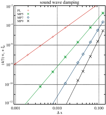
MM
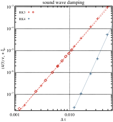
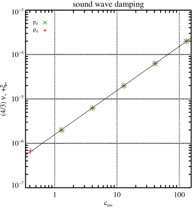
MM

Figure 1: Numerical dissipation of sound waves. Upper left panel: dependence on the grid resolution $\Delta x$ for different reconstruction schemes (PL/#S1, MP5/#S3, MP7/#S5, and MP9/#S6), the RK4 time integrator, and $C_{\mathrm{CFL}}=0.01$. Upper right panel: dependence on the size of the time step size $\Delta t$ for the RK3 (red; series #S7 and #S8) and RK4 (blue; series #S9) time integrators in simulations done with the MP9 scheme (so that spatial reconstruction errors are negligible). Different time steps were obtained by putting $C_{\mathrm{CFL}}=0.5$ and varying the grid resolution (plus symbols, dotted lines), or, additionally for the RK3 integrator, by keeping resolution fixed (i.e. $64$ zones) and varying the CFL factor (diamonds, dashed line). Lower left panel: dependence on the sound speed for two simulations series in which we kept the background density $\rho_{0}$ constant but varied the background pressure $p_{0}$ (#cS1, green crosses), and in which we kept $p_{0}$ constant but varied $\rho_{0}$ (#cS2, red plus signs). Lower right panel: dependence on the wavenumber $k=2\pi/\lambda$, i.e. on the box size (#cS3). The results shown in the two lower panels were obtained using $32$ zones, the MP5 scheme, the RK3 time integrator, and $C_{\mathrm{CFL}}=0.01$. Straight lines are fits to the simulation results.

With simulation series #S1, #S3, #S5, and #S6 (Tab. 1; upper left panel of Fig. 1), we investigated the influence of the reconstruction scheme on the numerical dissipation. To keep the contribution of the time integration errors as small as possible, we set $C_{\mathrm{CFL}}=0.01$. For every simulation, we measure the damping rate $\mathfrak{D}_{\mathrm{s}\ast}$ from the decay of the kinetic energy, from which we compute the numerical dissipation of the code according to Eq. (34) as

$$\frac{4}{3}\nu_{\ast}+\xi_{\ast}=\frac{2}{k^{2}}\mathfrak{D}_{\mathrm{s}\ast},$$ (35)

where the right hand side is given by the simulation results. Thus, in the case of sound waves, one cannot determine $\nu_{\ast}$ and $\xi_{\ast}$ separately from the value of $\mathfrak{D}_{\mathrm{s}\ast}$, but only a linear combination of both quantities. For every simulation series (i.e. reconstruction scheme), we fit the function

$$\ln\bigg{(}\frac{4}{3}\nu_{\ast}+\xi_{\ast}\bigg{)}=r\ln(\Delta x)+d,$$ (36)

where $r$ is the measured order of convergence of the scheme. From the fit parameter

$$d=\ln\left[\left(\frac{4}{3}\mathfrak{N}_{\nu}^{\Delta x}+\mathfrak{N}_{\xi}^{\Delta x}\right)\frac{\mathcal{V}}{\mathcal{L}^{r-1}}\right],$$ (37)

we can compute $\frac{4}{3}\mathfrak{N}_{\nu}^{\Delta x}+\mathfrak{N}_{\xi}^{\Delta x}$ if both the characteristic speed and the length of the system are known. As we will show below, for this test $\mathcal{L}=\lambda=1$ ($\lambda=2\pi/k$ being the wavelength) and $\mathcal{V}=c_{\mathrm{s}}=1.291$. The results presented in Tab. 1 and the upper right panel of Fig. 1 show that all schemes have an exponent $r$ close to the theoretical order $r_{\rm th}$ of the method.

The results of the simulation series #S2, #S3, and #S4 (Tab. 1) show that the LF, HLL and HLLD Riemann solvers damp sound waves very similarly.

With the simulation series #S7–#S9, we determine the contribution of the RK3 (#S7 and #S8) and RK4 (#S9) time integrators to the numerical dissipation. To keep the contribution of the spatial discretisation errors as low as possible, we use the MP9 reconstruction. We vary the timestep either by varying the grid resolution (keeping $C_{\mathrm{CFL}}=0.5$; series #S7 and #S9) or by varying the CFL factor (series #S8). According to Eq. (19), both approaches should be equivalent. In both cases, the RK3 scheme performs very close to third order accuracy, whereas the order of the RK4 integrator is higher than expected. We attribute the overperformance of RK4 in this test to the fact that it is not a TVD scheme since we have not computed the time-reversed operator $\tilde{L}$ as suggested in the Shu & Osher (1988) and in Suresh & Huynh (1997) for time integration schemes with order larger than three. However, the overperformance of RK4 in this test is very likely a fortunate coincidence (see Sec. 4.1.3, where it is not the case). The estimators $\frac{4}{3}\mathfrak{N}_{\nu}^{\Delta t}+\mathfrak{N}_{\xi}^{\Delta t}$ are obtained by employing a fitting procedure analogous to the one for $\frac{4}{3}\mathfrak{N}_{\nu}^{\Delta x}+\mathfrak{N}_{\xi}^{\Delta x}$ (see Tab. 1 and the upper right panel of Fig. 1).

The natural characteristic speed of this flow problem should be the sound speed ($\mathcal{V}=c_{\mathrm{s}}$). To test this hypothesis, we performed simulations varying the background pressure (series #cS1) or the density (#cS2) within the range given in Tab. 2. The results were fitted with the function

$$\ln\bigg{(}\frac{4}{3}\nu_{\ast}+\xi_{\ast}\bigg{)}=\alpha\ln(c_{\mathrm{s}})+d.$$ (38)

From the fit, we obtain the value of $\alpha$, expecting $\alpha=1$, and from the offset $d$, we determine $\mathfrak{N}_{\rm tot}^{\Delta x}=\mathfrak{N}_{\rm tot}^{\Delta x}=(4/3)\mathfrak{N}_{\nu}^{\Delta x}+\mathfrak{N}_{\xi}^{\Delta x}$ (Tab. 2). The table and the lower left panel of Fig. 1 clearly show that the sound speed is indeed the characteristic speed of the system.

To determine the characteristic length of the system (the natural candidate being the wavelength $\lambda$), we performed the simulation series #cS3 varying the wavelength $\lambda$ (and the size of the simulation domain accordingly, i.e. $L=\lambda$). The results were fitted with the function

$$\ln\bigg{(}\frac{4}{3}\nu_{\ast}+\xi_{\ast}\bigg{)}=\alpha\ln(\lambda)+d,$$ (39)

expecting again $\alpha=1$. Table 2 and the lower right panel of Fig. 1 confirm our hypothesis. The figure shows that the numerical viscosity term is proportional to $k^{-1}$, i.e. $D_{s*}/k^{2}\propto k^{-1}$ (see Eq. 34).

4.1.2 Alfvén Waves

With the help of Alfvén wave simulations, we determine a linear combination of the numerical shear viscosity and resistivity of the code. We set the background magnetic field and density to $b_{0x}=\rho_{0}=1$, the pressure to $p_{0}=2\times 10^{-3}$, and the transversal velocity to $\textsl{v}_{0y}=\textsl{v}_{0}=0$. We imposed a perturbation of the form

$$b_{1y}(x,0)=\epsilon\sin(kx),$$ (40)

$$\textsl{v}_{1y}(x,0)=-\frac{b_{y1}}{\sqrt{\rho_{0}}}.$$ (41)

In ideal MHD, an Alfvén wave propagates with a constant amplitude at the Alfvén speed $c_{\mathrm{A}}=b_{0x}/\sqrt{\rho_{0}}$. In the presence of viscosity and resistivity, the wave amplitude decreases with time. In the weak damping approximation, i.e. for $k^{4}(\nu+\eta)^{2}/(4c_{\mathrm{A}}^{2})\ll 1$, the velocity evolution reads (for the derivation, see Campos, 1999)

$$\textsl{v}_{y}(x,t)=\textsl{v}_{0}e^{-\mathfrak{D}_{\mathrm{A}}t}e^{ik(x\mp c_{\mathrm{A}}t)},$$ (42)

where the Alfvén damping rate is defined as

$$\mathfrak{D}_{\mathrm{A}}=\frac{k^{2}}{2}(\eta+\nu).$$ (43)

We verified Eq. (43) with the help of numerical simulations, and also checked that the bulk viscosity does not influence the damping coefficient (see Rembiasz, 2013, for details).

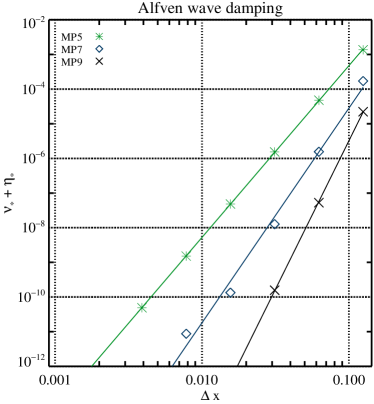
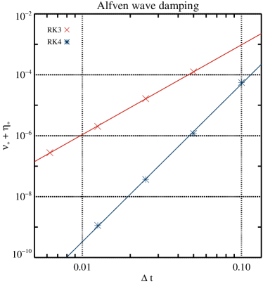
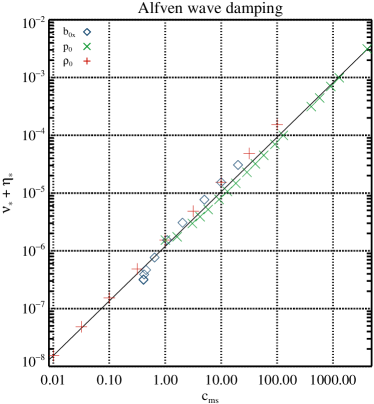
MM MM

Figure 2: Numerical dissipation of Alfvén waves. Upper left panel: dependence on the grid resolution $\Delta x$ for three different reconstruction schemes (MP5/#A2, MP7/#A3, and MP9/#A4) using RK4 and $C_{\mathrm{CFL}}=0.01$. Upper right panel: dependence on the time step size $\Delta t$ (changing the grid resolution but keeping $C_{\mathrm{CFL}}=0.8$) for two different time integrators (#A6, and #A7) using the HLL Riemann solver and MP9. Lower left panel: dependence on the fast magnetosonic speed for three simulation series varying the background magnetic field strength $b_{0x}$ (#cA1, blue diamonds), the background pressure $p_{0}$ (#cA2, green crosses), and the background density $\rho_{0}$ (#cA3, red plus signs) keeping all other parameters constant. Lower right panel: dependence on the wavenumber $k=2\pi/\lambda$, i.e. on the box size #cA4. Straight lines are fits to the simulation results.

In the simulation series #A2, #A4, and #A5 (see Tab. 1) we compared the influence of the MP5, MP7, and MP9 reconstruction schemes on the numerical shear viscosity $\nu_{\ast}$ and resistivity $\eta_{\ast}$. For every simulation, we measured the decrease of the kinetic energy, from which we determined a linear combination of the numerical shear viscosity and resistivity

$$\nu_{\ast}+\eta_{\ast}=\frac{2}{k^{2}}\mathfrak{D}_{\mathrm{A}\ast}.$$ (44)

The simulation results are fitted with the function

$$\ln(\nu_{\ast}+\eta_{\ast})=r\ln(\Delta x)+d,$$ (45)

where $r$ is the numerically measured order of accuracy of the reconstruction scheme. From the fit parameter $d$ and Eqs. (17), (21), and (44) we determined $\mathfrak{N}_{\nu}^{\Delta x}+\mathfrak{N}_{\eta}^{\Delta x}$. Table 1 and the upper left panel of Fig. 2 show that all methods have an order of convergence close to the theoretical expectation.

According to the results of the simulation series #A1, #A2, and #A3 (Tab. 1), the numerical dissipation of the LF, HLL, and HLLD Riemann solvers are also very similar for Alfvén waves.

With the simulation series #A6 and #A7 (upper right panel of Fig. 2), we assessed the contribution to the numerical dissipation of the RK3 and RK4 time integrators, respectively. We set $C_{\mathrm{CFL}}=0.8$ and changed the timestep by varying the grid resolution. The results presented in Tab. 1 and the upper right panel of Fig. 2 show that the RK3 time integrator performs at its theoretical order, whereas the order of the RK4 integrator is once again (like in the sound wave tests) higher than expected.

The characteristic velocity $\mathcal{V}$ for the Alfvén wave test problem can be inferred from simulation series #cA1, #cA2, and #cA3, in which we varied the magnetic field, pressure, and density, respectively. We find that the logarithm of the numerical dissipation determined from these simulation data can be fitted (see lower left panel of Fig. 2) by the function

$$\ln(\nu_{\ast}+\eta_{\ast})=\alpha\ln(c_{\mathrm{ms}})+d,$$ (46)

where $\alpha$ and $d$ are fitting parameters, and $c_{\mathrm{ms}}$ is the fast magnetosonic speed, which is is defined as

$$c_{\mathrm{ms}}=\sqrt{\frac{1}{2}\left(c_{\mathrm{A}}^{2}+c_{\mathrm{s}}^{2}+\sqrt{(c_{\mathrm{A}}^{2}+c_{\mathrm{s}}^{2})^{2}-4c_{\mathrm{A}}^{2}c_{\mathrm{s}}^{2}\cos^{2}\theta}\right)},$$ (47)

where $\theta$ is the angle between the perturbation wave vector and the background magnetic field. For a wavevector parallel to the background field ($\theta=0$)

$$c_{\mathrm{ms}}=\mathrm{max}\{c_{\mathrm{A}},c_{\mathrm{s}}\}.$$ (48)

The values of the fitting parameter $\alpha$, which are given in Tab. 2, confirm that the characteristic velocity $\mathcal{V}$ is the fast magnetosonic speed (not the Alfvén speed as one could have presumed), both in the flow regime where $\mathcal{V}$ is dominated by the Alfvén speed and the sound speed.

The simulation series #cA4 (Tab. 2) shows that the characteristic length of the Alfvén wave simulations is, as for the sound wave test, the wavelength, and that the numerical dissipation can be fitted by (see Tab. 2 and the lower right panel of Fig. 2)

$$\ln(\nu_{\ast}+\eta_{\ast})=\alpha\ln{\lambda}+d\,.$$ (49)

Finally, to investigate whether the errors resulting from spatial discretisation and time integration are additive, we performed simulations #A8, in which both types of errors should contribute non-negligibly to the numerical dissipation. Figure 3 shows the simulation results together with the expected numerical dissipation of the RK3 integrator (green), the MP5 scheme (blue), and the sum of both contributions (red). As the figure shows, the errors add linearly.

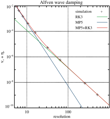
Figure 3: Numerical dissipation as a function of grid resolution for the MP5 reconstruction scheme and the RK3 time integrator with $C_{\mathrm{CFL}}=0.5$. The simulation results are marked with black plus signs. The straight lines depict the predicted numerical dissipation of the RK3 time integrator (green), the MP5 scheme (blue), and the sum of both types of numerical dissipation (red). For a grid resolution $\leq 16$ zones, Alfvén waves are mainly damped by spatial discretisation errors, and for $\geq 128$ zones by time integration errors. In the intermediate regime ($16\ldots 128$ zones), both types of errors add linearly (like proper scalars).

4.1.3 Magnetosonic Waves

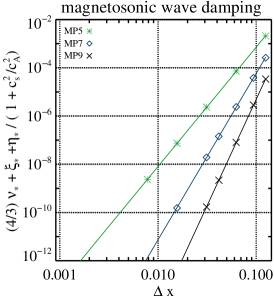
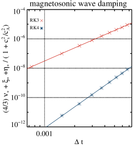
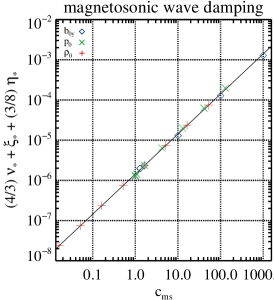
Figure 4: Numerical dissipation of magnetosonic waves. Left panel: dependence on the grid resolution $\Delta x$ for three different reconstruction schemes (MP5/#MS1, MP7/#MS2, and MP9/#MS3) using a HLL Riemann solver, RK4, and $C_{\mathrm{CFL}}=0.01$. Middle panel: dependence on the time step size $\Delta t$ for two different time integrators (RK3/#MS4 and RK4/#MS5) using the HLL Riemann solver, MP9, and a grid resolution of 64 zones. Right panel: dependence on the fast magnetosonic speed for simulations varying the background magnetic field strength $b_{0y}$ (#cMS1, blue diamonds), the background pressure $p_{0}$ (#cMS2, green crosses), and the background density $\rho_{0}$ (#cMS3, red plus signs) keeping all other parameters constant. Straight lines of are fits to the simulation results.

From the simulations of magnetosonic waves, we determine the numerical resistivity and viscosity of the Aenus  code. If not otherwise stated, the background pressure, density, and magnetic field strength are set to $p_{0}=\rho_{0}=b_{0y}=1$ and ${\bf b_{0}}=b_{0y}{\bf\hat{y}}$, respectively. We perturb the background by a magnetosonic wave of the form

$$\textsl{v}_{x1}(x,0) =\epsilon\sin(k_{x}x),$$ (50)

$$\textsl{v}_{y1}(x,0) =\textsl{v}_{x1}\frac{k_{x}^{2}b_{0x}b_{0y}}{b_{0x}^{2}k_{x}^{2}-\rho_{0}\omega^{2}},$$ (51)

$$b_{y1}(x,0) =\textsl{v}_{x1}\frac{k_{x}b_{0y}\omega\rho_{0}}{\rho_{0}\omega^{2}-b_{0x}^{2}k_{x}^{2}},$$ (52)

$$\rho_{1}(x,0) =\textsl{v}_{x1}\frac{k_{x}\rho_{0}}{\omega},$$ (53)

$$e_{1}(x,0) =\textsl{v}_{x1}\frac{k_{x}p_{0}\Gamma}{\omega(\Gamma-1)},$$ (54)

where $e_{1}$ is the total specific energy of the wave. The velocity amplitude $\epsilon=10^{-5}$, and the wave’s angular frequency $\omega$ is given by

$$\omega^{2}=k^{2}c_{\rm ms}^{2}.$$ (55)

For $\theta=\pi/2$ (a value chosen in almost all simulations) the magnetosonic speed reads (see Eq. 47)

$$c_{\mathrm{ms}}=\frac{\omega}{k}=\sqrt{\frac{{\bf b_{0}}^{2}+\Gamma p_{0}}{\rho_{0}}}.$$ (56)

In the presence of viscosity or resistivity, the wave will be damped with time, i.e. the $x$ component of the wave velocity will decrease as

$$\textsl{v}_{x}(x,t)=\epsilon\,e^{-\mathfrak{D}_{\mathrm{ms}}t}e^{ik(x\mp c_{\mathrm{ms}}t)},$$ (57)

where the damping coefficient for a fast magnetosonic wave propagating in the direction perpendicular to the background magnetic field is (for the derivation, see Campos, 1999)

$$\mathfrak{D}_{\mathrm{ms}}=\frac{k^{2}}{2}\left(\frac{4}{3}\nu+\xi+\frac{\eta}{1+c_{\mathrm{s}}^{2}/c_{\mathrm{A}}^{2}}\right).$$ (58)

We verified this equation numerically (see Rembiasz, 2013, for details).

We also performed simulations #MS1, #MS2, and #MS3 (Tab. 1) to investigate the influence of the MP5, MP7, and MP9 reconstruction schemes. From the measured kinetic energy damping, we determined a linear combination of the numerical resistivity, shear viscosity, and bulk viscosity, i.e.

$$\frac{4}{3}\nu_{\ast}+\xi_{\ast}+\frac{3}{8}\eta_{\ast}=\frac{2}{k^{2}}\mathfrak{D}_{{\rm ms}\ast}.$$ (59)

We fitted the simulation results with the function

$$\ln\left(\frac{4}{3}\nu_{\ast}+\xi_{\ast}+\frac{3}{8}\eta_{\ast}\right)=r\ln(\Delta x)+d,$$ (60)

where the fit parameter $r$ is the numerically measured order of the reconstruction scheme. From the fit parameter $d$, and with Eqs. (17), (20), (21), and (59), we determined the combination of coefficients $\frac{4}{3}\mathfrak{N}_{\nu}^{\Delta x}+\mathfrak{N}_{\xi}^{\Delta x}+\frac{8}{3}\mathfrak{N}_{\eta}^{\Delta x}$ (see Tab. 1 and left panel of Fig. 4).

Using simulation series #MS4 and #MS5, we studied the contribution of the RK3 and RK4 time integrators to the numerical dissipation (see Tab. 1 and middle panel of Fig. 4). We find that the RK4 integrator performs at a higher order than theoretically expected. Again, we point out that probably due to the non-TVD preserving property of our implementation of RK4, it overperformes in this test (see Sect. 4.1.2).

To determine the characteristic speed, we performed simulation series #cMS1, #cMS2 and #cMS3 varying background magnetic field strength, pressure, and density, respectively (Tab. 2). Hardly surprisingly, the characteristic speed is the fast magnetosonic speed (see bottom panel of Fig. 4), which is confirmed quantitatively with the help of the fit function

$$\ln\left(\frac{4}{3}\nu_{\ast}+\xi_{\ast}+\frac{3}{8}\eta_{\ast}\right)=\alpha\ln(c_{\mathrm{ms}})+d.$$ (61)

As expected, the fit (see Tab. 2) is consistent with $\alpha=1$ within the measurement errors. The value of $d$ can be used to estimate $\frac{4}{3}\mathfrak{N}_{\nu}^{\Delta x}+\mathfrak{N}_{\xi}^{\Delta x}+\frac{3}{8}\mathfrak{N}_{\eta}^{\Delta x}$. In the asymptotic regime $b_{0}\ll p_{0}$, the numerical damping is independent of the magnetic field strength, while it is proportional to the field strength for $b_{0}\gg p_{0}$.

4.1.4 Estimation of Numerical Resistivity and Viscosity

So far, we measured the numerical damping for three wave types separately. For each type of a wave, the damping coefficient depends on a linear combination of the resistivity, shear viscosity and bulk viscosity (see Eqs. 34, 43, and 58). This gives a system of three linearly independent equations with three unknowns, which has a unique solution.

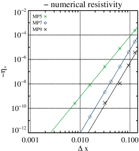
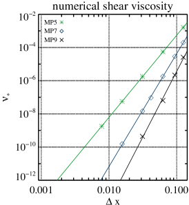
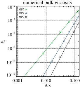
Figure 5: Fits of the numerical resistivity (left), shear viscosity (center), and bulk viscosity (right) computed from the combined damping rates of sound waves, Alfvén waves, and magnetosonic waves for three different reconstruction schemes. Note that the numerical resistivity is negative.

If we consider series of simulations in which time discretisation errors are negligible (as those in upper left panels of Figs. 1, 2, and 4), at a fixed grid resolution $k\Delta x=const.$ and for a given numerical method the numerical viscosity and resistivity should be the same according to our ansatz (Eqs.  17, 20, and 21). Therefore, the damping rates of the three propagating waves can (in principle) be used to compute the numerical viscosity and resistivity.

In Fig. 5 we present the resistivity, shear viscosity, and bulk viscosity for three different reconstruction schemes (MP5, MP5 and MP9) as a function of grid resolution. In all simulations we used the HLL Riemann solver, a RK4 time integrator, and $C_{\mathrm{CFL}}=0.01$. Fitting a power law to the data allows us to compute the coefficients entering in the ansatz given by Eqs. (17), (20), and (21). From the fit parameters, which can be found in Tab. 3, we compute the exponent $r$ appearing in the ansatz independently for resistivity and viscosity. For all three reconstruction schemes, (i) the values of $r$ are close to the expected order of convergence, $r_{\rm th}$, except for a small deviation in the case of MP9, and (ii) the value of the numerical viscosity is significantly larger than the absolute value of the numerical resistivity.

Our most striking result is that the value of the numerical resistivity $\eta_{*}$ is negative, its absolute value being about one order of magnitude smaller (and even two orders for MP9) than the value of the numerical viscosity (see Tab. 3). The value of the resistivity coefficient $\mathfrak{N}_{\eta}^{\Delta x}$ obtained with MP9 (providing the most accurate result) is compatible with a non-negative (very small) numerical resistivity, while the values of the numerical shear viscosity and bulk viscosity are positive and very similar. The resulting damping rate, which is a combination of resistivity and viscosity, prevented an amplification of the wave amplitude in all three systems studied. Taken together these facts suggest that the numerical viscosity must be considerably larger than the numerical resistivity of the code. Hence, we conjecture that there are large systematic uncertainties that prevent us from properly measuring the numerical resistivity of the code in all three wave propagation tests.

Given that the dissipation is dominated by viscosity rather than resistivity, we had to turn to a completely different system in order to study whether our ansatz for numerical resistivity is a valid one, and if true, whether the results are consistent with a positive value of the resistivity (see Sec. 4.3).

reconstruction	$\mathfrak{N}_{\eta}^{\Delta x}$	$r_{\eta}$	$\mathfrak{N}_{\nu}^{\Delta x}$	$r_{\nu}$	$\mathfrak{N}_{\xi}^{\Delta x}$	$r_{\xi}$
MP5	$-7.0\pm 0.5$	$4.94\pm 0.02$	$49\pm 3$	$4.95\pm 0.02$	$51\pm 4$	$4.95\pm 0.02$
MP7	$-41\pm 3$	$6.81\pm 0.03$	$270\pm 50$	$6.80\pm 0.06$	$354\pm 18$	$6.881\pm 0.017$
MP9	$\ \ -3\pm 6$	$6.8\pm 0.6$	$300\pm 200$	$7.9\pm 0.3$	$200\pm 200$	$7.7\pm 0.3$

Table 3: Values of the parameters in our ansatz for the spatial dependence of the numerical viscosity (Eqs. 17 and 20) and numerical resistivity (Eq. 21) based on a fit of the results shown in Fig. 5. Note that we obtain three different estimates of the exponent $r$ from fits of resistivity ($r_{\eta}$), shear viscosity ($r_{\nu}$), and bulk viscosity ($r_{\xi}$).

4.1.5 Waves with a Background Velocity

So far, in the wave damping simulations, we have set the background velocity to zero. To test whether a background velocity affects the numerical damping (i.e. by modifying the characteristic speed of the flow), we repeated the damping test for the sound waves, Alfvén, waves, and magnetosonic waves with a non-zero background velocity. All simulations were performed with the MP5 reconstruction scheme and the RK3 time integrator (with $C_{\mathrm{CFL}}=0.1$). For all three Riemann solvers and all types of waves we observed the same behaviour, i.e. the component of the background flow velocity that is perpendicular to the propagation of the wave ($\textsl{v}_{0y}$) does not affect the numerical dissipation, whereas the parallel component ($\textsl{v}_{0x}$) does. Figure 6 shows the numerical dissipation for some exemplary simulations of the sound wave damping test done with the HLL Riemann solver. Based on these simulations, we conclude that the characteristic speed of the flow is given by the sum of (the parallel component of) the flow velocity and the fast magnetosonic speed or, in other words, by the fast magnetosonic eigenvalue of the ideal MHD equations.

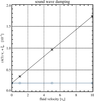
Figure 6: Numerical dissipation as a function of the flow velocity parallel (black asterisks) and perpendicular (blue diamonds) to the direction of the propagation of the sound wave. The simulations were performed with 32 zones, MP5, RK3 (with $C_{\mathrm{CFL}}=0.1$), and the HLL Riemann solver. Other solvers (LF and HLLD) exhibit a very similar behaviour.

4.2 Sound waves in 2D

So far, we have studied wave propagation problems in 1D. However, it is well known that unless a genuinely multi-D reconstruction algorithm is used (as proposed by, e.g.  Colella et al., 2011; McCorquodale & Colella, 2011; Zhang et al., 2011; Buchmüller & Helzel, 2014), the order of a reconstruction scheme can be reduced in simulations involving more than one spatial dimension. Our code Aenus employs several independent one-dimensional reconstruction steps (one per dimension). Thus, the convergence rate may be degraded to second order in multi-D simulations, i.e. well below that of 1D applications.

We studied this aspect with the help of 2D simulations (Tab. 4) of sound wave propagation in a box of size $L_{x}\times L_{y}$ with periodic boundary conditions in both directions. We set the background density and pressure to $\rho_{0}=p_{0}=1$, and imposed a perturbation of the form

$$\textsl{v}_{1x}(x,y,t=0) =\epsilon\sin(\theta)\sin(k_{x}x+k_{y}y),$$ (62)

$$\textsl{v}_{1y}(x,y,t=0) =\epsilon\cos(\theta)\sin(k_{x}x+k_{y}y),$$ (63)

$$\rho_{1}(x,t=0) =\frac{\epsilon}{c_{\mathrm{s}}}\rho_{0}\sin(k_{x}x+k_{y}y),$$ (64)

$$p_{1}(x,t=0) =\frac{\epsilon}{c_{\mathrm{s}}}\Gamma p_{0}\sin(k_{x}x+k_{y}y)$$ (65)

where $\Gamma=5/3$, $\epsilon=10^{-5}$, $\theta$ is an angle between the $x-$axis and the wavevector, ${\bf{k}}=(k_{x},k_{y}),$ where

$$k_{x} =\frac{2\pi}{L_{x}},$$ (66)

$$k_{y} =\frac{2\pi}{L_{y}}.$$ (67)

The wavelength is given by

$$\lambda=\frac{2\pi}{k}=\frac{2\pi}{\sqrt{k_{x}^{2}+k_{y}^{2}}}=\frac{L_{x}L_{y}}{\sqrt{L_{x}^{2}+L_{y}^{2}}}.$$ (68)

In all 2D simulations, we set $L_{x}=1$, like in all 1D sound wave simulations (but series #cS3) and use a uniform grid, i.e. $\Delta x=\Delta y$. Note that the 1D expressions are recovered in the limit $L_{y}\rightarrow\infty$. We determine numerical damping from the kinetic energy of sound waves whose time evolution is

$$E_{kin}(t)=E_{kin}(0)e^{-2\mathfrak{D}_{s}t}$$ (69)

in an analogous manner as described in Sec. 4.1.1. In the case of scalar constant bulk and shear viscosities, the damping rate $\mathfrak{D}_{s}$ is given by (analogically to the 1D case, Eq. 34)

$$\mathfrak{D}_{s}=\frac{k^{2}}{2}\left(\frac{4}{3}\nu+\xi\right)=\frac{k_{x}^{2}+k_{y}^{2}}{2}\left(\frac{4}{3}\nu+\xi\right).$$ (70)

However, as already mentioned in Sec. 2.3 (see Eq. 24), numerical viscosities have a tensorial character in a multi-D simulation, hence the damping rate is given by

$$\mathfrak{D}_{s} =\frac{1}{2}{\bf k}^{T}\left(\frac{4}{3}\bm{\nu}_{\ast}+\bm{\xi}_{\ast}\right){\bf k}=$$

$$=\frac{1}{2}\Bigg{[}k_{x}^{2}\left(\frac{4}{3}\nu_{\rm sp}^{xx}+\xi_{\rm sp}^{xx}\right)+k_{y}^{2}\left(\frac{4}{3}\nu_{\rm sp}^{yy}+\xi_{\rm sp}^{yy}\right)+k^{2}\left(\frac{4}{3}\nu_{t}+\xi_{t}\right)\Bigg{]}.$$ (71)

To be able to determine (linear combinations of) $\mathfrak{N}_{\nu}^{\Delta x},\mathfrak{N}_{\xi}^{\Delta x},\mathfrak{N}_{\nu}^{\Delta x}$ and $\mathfrak{N}_{\xi}^{\Delta x}$ (defined in Eqs. 17 and 20), i.e. $\mathfrak{N}_{\rm tot}^{\Delta x}=(4/3)\mathfrak{N}_{\nu}^{\Delta x}+\mathfrak{N}_{\xi}^{\Delta x}$ and $\mathfrak{N}_{\rm tot}^{\Delta t}=(4/3)\mathfrak{N}_{\nu}^{\Delta t}+\mathfrak{N}_{\xi}^{\Delta t}$ (Tab. 4), we first need to identify the characteristic velocities $\mathcal{V}_{x},\mathcal{V}_{y}$ and $\mathcal{V}$, and lengths $\mathcal{L}_{x},\mathcal{L}_{y}$ and $\mathcal{L}$ of the system. From our studies in 1D, we infer that the former must be the sound speed, which is homogenous and isotropic in the whole system and, thereby, $\mathcal{V}_{x}=\mathcal{V}_{y}=\mathcal{V}=c_{\mathrm{s}}$. Moreover, we postulate that $\mathcal{L}_{x}=2\pi/k_{x}$ and $\mathcal{L}_{y}=2\pi/k_{y}$, since for the reconstruction scheme in each dimensional sweep, this 2D sound wave problem reduces to a 1D wave propagation (e.g. Eq. 62 reduces to Eq. 50 for $y=\rm{const.}$). The characteristic (physical) time scale of the system is $\mathcal{T}=c_{\mathrm{s}}/\lambda$. And since the time integration errors must be proportional to $\Delta t/\mathcal{T}$, we conclude that $\mathcal{L}=\lambda$.

Therefore, for our system, ansatzes for $\nu_{\rm sp}^{xx}$ and $\nu_{t}$ (see Eqs.  25 and 27) read

$$\nu_{\rm sp}^{xx} =\mathfrak{N}_{\nu}^{\Delta x}c_{\mathrm{s}}\frac{2\pi}{k_{x}}\left(\frac{k_{x}\,\Delta x}{2\pi}\right)^{r},$$ (72)

$$\nu_{t} =\mathfrak{N}_{\nu}^{\Delta t}c_{\mathrm{s}}\lambda\left(\frac{c_{\mathrm{s}}\,\Delta t}{\lambda}\right)^{q}.$$ (73)

The ansatzes for the other components of numerical viscosities have an analogous form. Finally, the damping rate for 2D wave simulations is

$$\begin{split}\mathfrak{D}_{s}&=2\pi^{2}c_{\mathrm{s}}\left\{\left[(4/3)\mathfrak{N}_{\nu}^{\Delta x}+\mathfrak{N}_{\xi}^{\Delta x}\right]\left[\left(\frac{k_{x}}{2\pi}\right)^{r+1}(\Delta x)^{r}+\left(\frac{k_{y}}{2\pi}\right)^{r+1}(\Delta y)^{r}\right]\vphantom{\left[(4/3)\mathfrak{N}_{\nu}^{\Delta t}+\mathfrak{N}_{\xi}^{\Delta t}\right]\left[\left(\frac{k}{2\pi}\right)^{q+1}C_{\mathrm{CFL}}^{q}(\Delta x)^{q}\right]}\right.\\ &+\left.\left[(4/3)\mathfrak{N}_{\nu}^{\Delta t}+\mathfrak{N}_{\xi}^{\Delta t}\right]\left[\left(\frac{k}{2\pi}\right)^{q+1}C_{\mathrm{CFL}}^{q}(\Delta x)^{q}\right]\right\},\end{split}$$ (74)

which for an equidistant grid, i.e. $\Delta x=\Delta y$, and $L_{x}=1$, further simplifies to

$$\begin{split}\mathfrak{D}_{s}&=2\pi^{2}c_{\mathrm{s}}\left\{\left[(4/3)\mathfrak{N}_{\nu}^{\Delta x}+\mathfrak{N}_{\xi}^{\Delta x}\right]\left[(\Delta x)^{r}\left(1+L_{y}^{-r-1}\right)\right]\vphantom{\left[(4/3)\mathfrak{N}_{\nu}^{\Delta t}+\mathfrak{N}_{\xi}^{\Delta t}\right]\left[\left(1+L_{y}^{-2}\right)^{(1+q)/2}C_{\mathrm{CFL}}^{q}(\Delta x)^{q}\right]}\right.\\ &+\left.\left[(4/3)\mathfrak{N}_{\nu}^{\Delta t}+\mathfrak{N}_{\xi}^{\Delta t}\right]\left[\left(1+L_{y}^{-2}\right)^{(1+q)/2}C_{\mathrm{CFL}}^{q}(\Delta x)^{q}\right]\right\}.\end{split}$$ (75)

According to the above equation, for simulations in which numerical dissipation is dominated either by spatial reconstruction errors (series #LS1–#LS11 from Tab. 4) or by time integration errors (series #LS12–#LS17), the dissipation rate should respectively be $\left(1+L_{y}^{-r-1}\right)$ and $\left(1+L_{y}^{-2}\right)^{(1+q)/2}$ times larger than in the corresponding 1D simulations (with the same $L_{x}=1)$. Note that this difference between 1D and 2D simulations is due to the small change in the value of $\lambda$. Deviations from this expected value would be indicative of differences in the dissipation coefficients between 1D and 2D simulations. For the MP5 reconstruction scheme, assuming $r=5$, and boxes with $L_{y}=1,1.125$ and $1.25$, the dissipation should be respectively $2,1.49$ and $1.26$ times larger than in the 1D case, whereas in boxes with $L_{y}=2$ and $3$, the numerical dissipation rate should be basically equal to the 1D case (i.e. merely greater by a factor of $1.016$ and $1.001$, respectively). The upper panel of Fig. 7 depicts (in red) the damping rates in simulation series #LS1, #LS4, #LS5, #LS6, and #LS9 (Tab. 7) performed with the MP5 reconstruction scheme in 2D boxes of those sizes. The ratios of these damping rates to the damping rates in 1D (simulation series #S3 from Tables 1 and 4, marked with asterisks in the figure) are in a very good agreement with the above estimates. Similarly, we expect twice higher dissipation rates in simulations done with MP7 (series #LS2) and MP9 (series #LS3) reconstruction schemes in boxes with $L_{y}=1$ than in their 1D counterparts (simulation series #S5 and #S6, respectively), and basically equal (to the 1D case) dissipation rates in simulations with $L_{y}=2$ and $L_{y}=3$ (simulation series #LS7, #LS8, #LS10, and #LS11). Indeed, dissipation rates presented in the upper panel of Fig. 7 exhibit this behaviour.

In the above analysis, we implicitly assumed that $r,\,\mathfrak{N}_{\nu}^{\Delta x}$, etc. are equal in 1D and 2D simulations, so the previous analysis only provides a consistency check. However, these coefficients can actually be measured in 2D simulations and can be compared with the coefficients obtained for the 1D case. In Table 4, we present estimators for these quantities determined in the 2D simulations from dissipation rates with the help of Eq. (75) in an analogous way as described in Sec.  4.1.1. The estimators are indeed equal within the measurement errors for each reconstruction scheme, i.e. MP5, MP7 and MP9, in 1D and in 2D simulations. This signifies that our ansatzes (24)–(27) are correct at least for 2D wave simulations for the spatial reconstruction errors.

The bottom panel of Fig. 7 depicts dissipation rates in simulations series #LS12–#LS17 (Tab. 4) performed with the MP9 reconstruction scheme (so that spatial discretisation errors are negligible), $C_{\mathrm{CFL}}=0.5$, and RK3 (red) or RK4 (blue) time integrators in 2D boxes with $L_{y}=1$, $2$ and $3$ as well as in 1D (series #S7 and #S9). The estimators for $q$ and $\mathfrak{N}_{\rm tot}^{\Delta t}$ determined from these data are presented in Tab. 4. The RK3 time integration scheme once again (like in 1D) has its theoretical order, i.e. $q\approx 3$, whereas the RK4 time integrator once again overperforms by one unit the expected order, i.e. $q\approx 5$. The estimators for $\mathfrak{N}_{\rm tot}^{\Delta t}$ and $q$ for the RK3 scheme are very similar in 1D and 2D simulations, whereas for the RK4 scheme, there is a discrepancy, which cannot be explained by the measurement errors (i.e. $\mathfrak{N}_{\rm tot}^{\Delta t}$ ranges from $17\pm 3$ to $71\pm 32$, and $q$ from $5.14\pm 0.05$ to $5.5\pm 0.2$). Note, however, that this discrepancy is insignificant in the considered range of $\Delta t$ as there is a clear correlation between $q$ and $\mathfrak{N}_{\rm tot}^{\Delta t}$, i.e. the larger $q$, the larger $\mathfrak{N}_{\rm tot}^{\Delta t}$, leading to very similar predictions for the dissipation rate as we show in the next paragraph. Therefore, we conclude that our ansatzes (24)–(27) are valid for time integration errors in 2D and that both RK3 and RK4 time integration schemes perform (basically) identically in 1D and 2D simulations (with various box sizes).

Based on Eq. (75), we can make the following estimates for simulations where time integrator errors are dominant. For simulations done with RK3, assuming $q=3$ (and equal $\mathfrak{N}_{\rm tot}^{\Delta t}$), in a box with $L_{y}=1,2$ and $3$ (series #LS12, #LS14 and #LS16, respectively) numerical dissipation should be respectively $4,1.56$ and $1.23$ times greater than in 1D simulations (series #S7). For analogous simulations done with RK4 (series #LS13, #LS15 and #LS17, respectively), assuming $q=5$ (and equal $\mathfrak{N}_{\rm tot}^{\Delta t}$), the dissipation rates should respectively be $8,1.95,1.37$ greater than in the 1D case (series #S9). As can be seen in the bottom panel of Fig.  7, these predictions agree very well with our simulation results.

Table 4: Sound wave damping in 2D simulations (series #LS). Additionally, for the reader’s convenience, we repeat some 1D simulations (series #S) from Tab.  1. The columns give (from left to right) the series identifier, the $L_{y}$ box length ($L_{x}=1$), the reconstruction scheme, the Riemann solver, the time integrator, and the CFL factor. In all 2D simulations, an uniform grid is used (i.e. $\Delta y=\Delta x$) and the number of grid zones $N_{x}$ per $L_{x}$ is in the range from $8$ to $32$. The estimator for $\mathfrak{N}_{\rm tot}^{\Delta x}$, $r$, $\mathfrak{N}_{\rm tot}^{\Delta t}$, and $q$ (see Eqs. 17 and 20) is obtained from linear fits to the simulation results. For sound waves, $\mathfrak{N}_{\rm tot}^{\Delta x}=(4/3)\mathfrak{N}_{\nu}^{\Delta x}+\mathfrak{N}_{\xi}^{\Delta x}$ and $\mathfrak{N}_{\rm tot}^{\Delta t}=(4/3)\mathfrak{N}_{\nu}^{\Delta t}+\mathfrak{N}_{\xi}^{\Delta t}$.

series	$L_{y}$	Reco	Riemann	time	CFL	$\mathfrak{N}_{\rm tot}^{\Delta x}$	$r$	$\mathfrak{N}_{\rm tot}^{\Delta t}$	$q$
#LS1	$1$	MP5	HLL	RK3	$0.01$	$37.1\pm 2.6$	$4.90\pm 0.02$	$-$	$-$
#LS2	$1$	MP7	HLL	RK3	$0.01$	$273\pm 21$	$6.86\pm 0.03$	$-$	$-$
#LS3	$1$	MP9	HLL	RK3	$0.01$	$440\pm 300$	$8.2\pm 0.2$	$-$	$-$
#LS4	$1.125$	MP5	HLL	RK3	$0.01$	$33.7\pm 4.4$	$4.86\pm 0.02$	$-$	$-$
#LS5	$1.25$	MP5	HLL	RK3	$0.01$	$37\pm 7$	$4.90\pm 0.04$	$-$	$-$
#LS6	$2$	MP5	HLL	RK3	$0.01$	$37.2\pm 2.7$	$4.90\pm 0.02$	$-$	$-$
#LS7	$2$	MP7	HLL	RK3	$0.01$	$276\pm 24$	$6.86\pm 0.03$	$-$	$-$
#LS8	$2$	MP9	HLL	RK3	$0.01$	$570\pm 370$	$8.3\pm 0.2$	$-$	$-$
#LS9	$3$	MP5	HLL	RK3	$0.01$	$37.1\pm 2.5$	$4.90\pm 0.02$	$-$	$-$
#LS10	$3$	MP7	HLL	RK3	$0.01$	$277\pm 24$	$6.86\pm 0.03$	$-$	$-$
#LS11	$3$	MP9	HLL	RK3	$0.01$	$680\pm 360$	$8.35\pm 0.18$	$-$	$-$
#S3	$-$	MP5	HLL	RK4	$0.01$	$43.4\pm 2.5$	$4.962\pm 0.0141$	$-$	$-$
#S5	$-$	MP7	HLL	RK4	$0.01$	$302\pm 20$	$6.897\pm 0.021$	$-$	$-$
#S6	$-$	MP9	HLL	RK4	$0.01$	$830\pm 340$	$8.42\pm 0.15$	$-$	$-$
#LS12	$1$	MP9	HLL	RK3	$0.5$	$-$	$-$	$1.28\pm 0.04$	$2.94\pm 0.01$
#LS13	$1$	MP9	HLL	RK4	$0.5$	$-$	$-$	$17\pm 3$	$5.14\pm 0.05$
#LS14	$2$	MP9	HLL	RK3	$0.5$	$-$	$-$	$1.4\pm 0.2$	$2.970\pm 0.005$
#LS15	$2$	MP9	HLL	RK4	$0.5$	$-$	$-$	$31\pm 9$	$5.3\pm 0.1$
#LS16	$3$	MP9	HLL	RK3	$0.5$	$-$	$-$	$1.56\pm 0.01$	$2.978\pm 0.002$
#LS17	$3$	MP9	HLL	RK4	$0.5$	$-$	$-$	$46\pm 17$	$5.38\pm 0.13$
#S7	$-$	MP9	HLL	RK3	$0.5$	$-$	$-$	$1.492\pm 0.013$	$2.985\pm 0.002$
#S9	$-$	MP9	HLL	RK4	$0.5$	$-$	$-$	$71\pm 32$	$5.5\pm 0.2$

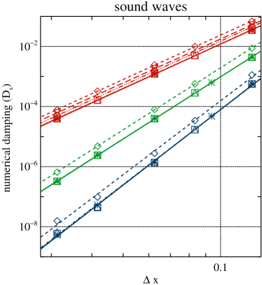
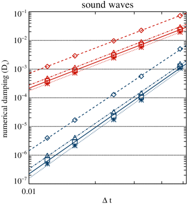
Figure 7: Numerical damping in sound wave simulations performed with the HLL Riemann solver in 1D (asterisks, dotted lines), and in 2D with $L_{y}=1$ (diamonds, dashed lines) , $L_{y}=1.125$ (downwards triangles, dash-dot-dot-dot line), $L_{y}=1.25$ (circles, long-dashed line), $L_{y}=2$ (upwards triangles, dashed-dotted lines) and $L_{y}=3$ (squares, solid lines). Top: simulations done with the RK3 time integrator with $C_{\mathrm{CFL}}=0.01$ (so that the time integration errors are negligible) and the MP5 (red), MP7 (green) and MP9 (blue) reconstruction schemes. Bottom: simulations done with the MP9 reconstruction scheme (so that time discretisation errors are negligible) and the RK3 (red) and RK4( blue) time integrators with $C_{\mathrm{CFL}}=0.5$. See also Tab. 4.

4.3 Tearing Mode Tests

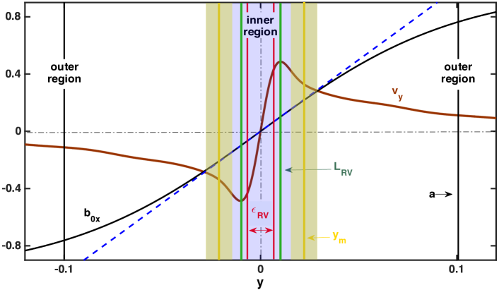
Figure 8: Background magnetic field, $b_{0x}$, (black; Eq. 76) and the amplitude (rescaled for a better visibility) of the velocity perturbation $v_{y}$ (brown; Eq. 94) of a TM. Only the central part of the computational domain is shown, i.e. $y\in[-0.15,0.15]$. In the outer region (white) and the inner region (blue) $v_{y}$ is given by Eqs. (A9) and (A22), respectively. In an intermediate region (shaded yellow) both solutions are valid and must be matched at a certain matching point, $y_{\mathrm{m}}$, within this region (yellow vertical line). Black, green, and red vertical lines respectively mark, the shear width $a$, the width of the resistive viscous layer $L_{\rm RV}$ (Eq. 92), and the point where $y=\epsilon_{\rm RV}$ (defined in Eq. A28). In the inner region, the Taylor expansion $b_{0x}(y)\approx b_{0}y/a$ (Eq. 85) is used to obtain the analytical solution (see Appendix A.1). The blue dashed line depicts the function $b_{0}y/a$ (with $b_{0}=1$) to illustrate the regime of the validity of the Taylor expansion.

The TM instability is a resistive MHD instability that can develop in current sheets, where, as a direct consequence of Ampère’s law, the magnetic field changes direction. TMs dissipate magnetic energy into kinetic energy and subsequently into thermal energy, disconnect and rejoin magnetic field lines, thereby changing the topology of the magnetic field. The linear theory of TM was extensively studied, in the context of plasma fusion physics, in a seminal paper by FKR63. TMs are of great relevance in astrophysics, (e.g. in the magnetopause or magnetotail of the solar wind, in flares or coronal loops of the Sun, and in the flares of the Crab pulsar (cf. Priest & Forbes, 2007; Pucci & Velli, 2014). They have also been suggested to be a terminating agent of the MRI (Balbus & Hawley, 1991; Latter et al., 2009; Pessah, 2010, but see Rembiasz et al. 2016a who observed an MRI termination by the Kelvin-Helmholtz instability in their 3D MRI simulations).

In this section, we present a test involving TMs, for which we know how the reconnection rate depends on the relevant parameters (resistivity, viscosity, etc.). By performing numerical simulations of viscous, but non-resistive MHD flows at different grid resolutions with various numerical methods, we developed a method to measure the numerical resistivity of MHD codes.

4.3.1 Theory

In this section, we sketch how to analytically obtain a growth rate and an instability criterion of the TM instability, leaving out all technical details which can be found in Appendix A.1. Many of the results presented here were already obtained by FKR63, or they are different limits of expressions found in that work.

Consider a two dimensional flow in the $x$-$y$ plane of constant background density $\rho_{0}=1$ threaded by a magnetic field

$$b_{0x}=b_{0}\tanh(y/a),$$ (76)

where $b_{0}$ is the magnetic field strength and $a$ defines the shear length (see Fig. 8). This magnetic field configuration gives rise to a current sheet at $|y/a|\lesssim 1$. To balance the resulting magnetic pressure gradient, one can introduce either a gas pressure gradient, so that $\nabla_{y}(p+b_{0x}^{2}/2)=0$ (pressure equilibrium configuration), or an additional magnetic field component, so that $\nabla_{y}(b_{0x}^{2}/2+b_{0z}^{2}/2)=0$ (force-free configuration). Both equilibrium configurations are stable in ideal MHD, but are TM unstable in resistive MHD.

FKR63 derived the instability criterion and the growth rate using the linearised resistive-viscous MHD equations in the incompressible limit, which read

$$\partial_{t}{\bf b} = \nabla\times({\bf v_{1}}\times{\bf b_{0}})+\eta\nabla^{2}{\bf b},$$ (77)

$$\rho_{0}\partial_{t}{\bf v_{1}} = -\nabla p+(\nabla\times{\bf b_{1}})\times{\bf b_{0}}+(\nabla\times{\bf b_{0}})\times{\bf b_{1}}$$ (78)

$$+\rho_{0}\nu\nabla^{2}{\bf v_{1}},$$

$$\nabla\cdot{\bf v} = 0,$$ (79)

$$\nabla\cdot{\bf b} = 0,$$ (80)

where ${\bf v}={\bf v_{0}}+{\bf v_{1}}$, ${\bf b}={\bf b_{0}}+{\bf b_{1}}$ and we denote background and perturbed quantities with subscripts ”$0$” and ”$1$”, respectively. In the incompressible limit, $|{\bf v_{1}}|\ll c_{s}$ holds, which was used to obtain the linearised equations. To simplify the notation, we omit hereafter the subscript “$1$” for the velocity perturbations, because the background flow is assumed to be at rest.

FKR63 solved the above equations using a WKB ansatz, i.e.

$$\textsl{v}_{y}(x,y,t) =\textsl{v}(y)e^{ikx+\gamma t},$$ (81)

$$b_{1y}(x,y,t) =b_{1}(y)e^{ikx+\gamma t},$$ (82)

where $k$ is the wavevector in the $x$ direction, and $\gamma$ is the growth rate of the TM instability. This ansatz is justified only if the time dependence of the background magnetic field can be neglected. This is the case when the diffusion time scale is much larger than the instability time scale, i.e. $a^{2}/\eta\gg\gamma^{-1}$. The Alfvén crossing time must be sufficiently short too, i.e. $a/c_{\mathrm{A}}\ll\gamma^{-1}$, which is equivalent to considering instantaneous propagation of Alfvén waves through the system. Combining both conditions, we have

$$\frac{a^{2}}{\eta}\gg\gamma^{-1}\gg\frac{a}{c_{\mathrm{A}}}.$$ (83)

Among other cases, FKR63 also considered perturbations whose wavelengths in the $x$ direction are comparable to (but smaller than) the shear width, i.e.

$$k\lesssim a^{-1}.$$ (84)

For such perturbations, the wavevectors may differ from that of the fastest growing mode appreciably, and it is possible to set up a numerical test in which, for a given grid resolution, both the magnetic shear layer and the TM are well resolved.

FKR63 solved the TM problem in the limit (84) with a so-called boundary layer analysis (BLA; for details see Appendix A.1). They define an inner region (see Fig.8) where resistive effects are important. We call this region the resistive layer of width $L_{\mathrm{R}}$ or, if the flow is also viscous, the resistive-viscous layer of width $L_{\mathrm{RV}}$. Far away from this layer, $|y|\gg L_{\mathrm{R}}$ or $|y|\gg L_{\mathrm{RV}}$, there is an outer region (see Fig. 8) where resistivity can be ignored and the ideal MHD equations are valid. The layer width $L_{\mathrm{R}}$ or $L_{\mathrm{RV}}$ can be expressed in terms of the physical parameters of the system (see Appendix A). The velocity perturbation $v_{y}(x,y,t)$ of the WKB ansatz (Eq. 81) exhibits two extrema at $y=\pm L_{\mathrm{R}}$ or $y=\pm L_{\mathrm{RV}}$ (see Fig. 8). Because the location of these extrema can be determined from our simulation results, the layer width $L_{\mathrm{R}}$ or $L_{\mathrm{RV}}$ is an appropriate quantity to compare simulation and theory.

In the BLA, the inner solution of the resistive MHD equations in a linearised background, i.e.

$$b_{0x}(y)\approx b_{0}y/a.$$ (85)

(which holds for $|y|\ll a$; blue dashed line in Fig. 8), is matched with the ideal MHD solution in the outer region at some matching point $|y_{\mathrm{m}}|$. The coordinate $y_{\mathrm{m}}$ has to fulfill the condition $L_{\mathrm{R}}\ll|y_{\mathrm{m}}|\ll a$ (or $L_{\mathrm{RV}}\ll|y_{\mathrm{m}}|\ll a$), which implies that these transition region can exist only if

$$L_{\mathrm{R}}\ll a\qquad\text{or}\qquad L_{\mathrm{RV}}\ll a.$$ (86)

In the inviscid limit, analytic TM solutions of the resistive MHD equations can be obtained. For the background magnetic field given by Eq. (76), TM will grow if

$$a\,k<1\ \ \ \mathrm{(instability)}.$$ (87)

In this case, the growth rate of the TM is

$$\gamma=1.82\eta^{3/5}\left(\frac{b_{0}k}{\sqrt{\rho_{0}}}\right)^{2/5}a^{-6/5}\left(\frac{1}{a\,k}-a\,k\right)^{4/5},$$ (88)

and the width of the resistive layer is according to our definition

$$L_{\mathrm{R}}=1.40\eta^{2/5}\left(\frac{\sqrt{\rho_{0}}}{b_{0}k}\right)^{2/5}a^{1/5}\left(\frac{1}{a\,k}-a\,k\right)^{1/5}$$ (89)

(see equations A24 and A25, respectively).

The growth rate given by Eq. (88) is of little value for our purpose, since it is obtained in the inviscid limit. However, as we have argued in section 2, both numerical viscosity and resistivity are an unavoidable result of the discretisation of the equations. Hence, if we want to use TMs to measure numerical resistivity, we have to use an approach which takes into account numerical viscosity as well. FKR63 also considered the resistive-viscous case for Prandtl numbers

$$P_{\mathrm{m}}\equiv\frac{\nu}{\eta}\gtrsim 1,$$ (90)

in the limit $k\ll a^{-1}$. Based on their approach, we obtained the TM growth rate for wavenumbers $k\lesssim a^{-1}$ (see Eq. A30)

$$\gamma\approx 0.84\eta^{5/6}\nu^{-1/6}\left(\frac{b_{0}k}{\sqrt{\rho_{0}}}\right)^{1/3}a^{-4/3}\left(\frac{1}{a\,k}-a\,k\right),$$ (91)

and the width of the resistive-viscous layer

$$L_{\mathrm{RV}}\sim(\eta\nu)^{1/6}\left(a\frac{\sqrt{\rho_{0}}}{b_{0}k}\right)^{1/3}.$$ (92)

These expressions should be useful to set up a test to measure numerical resistivity. However, as we will show in the next sections, it is difficult to find a region in the numerical parameter space where Eq. (91) holds, i.e. where Eqs. (84), (83), (86), and (90) are fulfilled.

4.3.2 Numerical Simulations of Physical TM

To demonstrate the possibility of using a TM simulation to measure numerical resistivity, we first set up the test using physical resistivity. This allows us to estimate the reconnection rate as a function of physical resistivity and viscosity.

Our numerical experiment is based on Landi et al. (2008), who were mainly interested in the non-linear phase of TM, i.e. the formation of magnetic islands and the onset of turbulence. Since we want to study the exponential growth of a single TM in detail, we modified their setup for our purposes. We used a computational box of size $[-L_{x},L_{x}]\times[-L_{y},L_{y}]$, where $L_{x}=L_{y}=\pi/3$, with periodic and open boundary conditions in $x$ and $y$ direction, respectively. We set the density and pressure to $\rho_{0}=p_{0}=1$, and used an ideal-gas EOS with $\Gamma=5/3$. In the expression for the background field, Eq. (76), we set $b_{0}=1$ and $a=0.1$.

We tested both the pressure equilibrium and force-free configurations and found that only the latter is suitable for our numerical experiments (see Rembiasz, 2013, for details). To obtain the force-free configuration we set

$$b_{0z}=\frac{b_{0}}{\cosh(y/a)}.$$ (93)

We note that our initial perturbations differ from those of Landi et al. (2008). As those authors only perturbed the velocity, the TM instability is triggered promptly for high resistivities only ($\eta\geq 10^{-5}$). Instead, we perturb both the velocity and the magnetic field based on an analytic solution of the TM:

$$\textsl{v}_{y}(x,y,t=0) =\textsl{v}(y)\sin(kx),$$ (94)

$$b_{1y}(x,y,t=0) =b_{1}(y)\cos(kx).$$ (95)

The function $\textsl{v}(y)$ is given by Eqs. (A9) and (A22) for $|y|\geq y_{\mathrm{m}}$ and $|y|\leq y_{\mathrm{m}}$, respectively, where $y_{\mathrm{m}}$ is the matching point (typically $y_{\mathrm{m}}=2L_{\mathrm{RV}}$). Landi et al. (2015) used similar perturbations, i.e. eigenfunctions of the TM, in their studies of what they called “an ideal TM”. This ideal case is a solution of the TM problem in a regime first studied by FKR63, but different from the one we consider here.

The function $b_{1}(y)$ in Eq. (95) is given by Eq. (A8) for $|y|\geq y_{\mathrm{m}}$, and it is constant for $|y|\leq y_{\mathrm{m}}$, i.e. $b_{1}(y\leq y_{\mathrm{m}})=b_{1}(y_{\mathrm{m}})$ according to the constant $\psi$ approximation (see Appendix A). The remaining perturbations $v_{1x}(x,y,t=0)$ and $b_{1x}(x,y,t=0)$ are determined from the divergence free conditions $\nabla\cdot{\bf b}=\nabla\cdot{\bf v}=0$. To reduce the computational cost, we chose the value of $k$ in such a way that exactly one TM fits into the box, i.e. $k=3$.

To compare the results of our TM simulations with the analytical predictions of Eqs. (91) and (92) for the TM growth rate and the width of the resistive viscous layer, respectively, we must ensure that we are in the regime of applicability of these analytical predictions, i.e. Eqs. (84), (83), (86), and (90) should be fulfilled. The first condition (Eq. 84) is ensured by our choice of $k$ and $a$. The other conditions can be written as

$$\mathcal{C}_{1}\equiv \,\gamma a^{2}\eta^{-1}\gg 1,$$ (96)

$$\mathcal{C}_{2}\equiv \,a^{-1}c_{\mathrm{A}}\gamma^{-1}\gg 1,$$ (97)

$$\mathcal{C}_{3}\equiv \,aL_{\mathrm{R}V}^{-1}\gg 1,$$ (98)

$$P_{\mathrm{m}}\equiv \,\nu\eta^{-1}\gtrsim 1.$$ (99)

We plot iso-contours of these four quantities in the $\eta$-$\nu$ plane (see Fig. 9) to locate the region where the analytical expressions are valid.

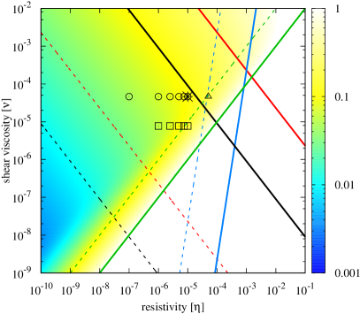
Figure 9: Parameter space of our numerical TM simulations and validity limits of the analytical expression for the growth rate $\gamma$ given by Eq. (91). The color map gives the value of the quantity $(C_{1}^{-2}+C_{2}^{-2}+C_{3}^{-2}+0.01P_{\rm m}^{-2})^{1/2}$, and the red, blue, and black solid and dashed lines show the locations where $\mathcal{C}_{1}$, $\mathcal{C}_{2}$, and $\mathcal{C}_{3}$ (see Eqs. 96 - 98) have a constant value of $10$ and $100$, respectively. Solid and dashed green lines show the locations where $P_{\mathrm{m}}$ has a value $0.1$ and $1$, respectively. Symbols indicate the parameter values obtained for the reference simulation #Rf (asterisk), and the simulations #TMa (circles), #TMc (squares), and #TMc (triangles). In the blue shaded region the conditions given by Eqs. (96) - (98) are satisfied best.

We first discuss the results of a simulation with $\eta=10^{-5}$ and $\nu=10^{-4}$, which we call reference model (#Rf) and which is marked by an asterisk in Fig. 9. The first condition (Eq. 96) is only marginally satisfied for the reference model ($\mathcal{C}_{1}\approx 25$). To improve the situation, one should decrease the resistivity and viscosity, i.e. one should increase the grid resolution. This would place the model towards the lower left corner of Fig. 9, where all the conditions are better satisfied. Therefore, we are limited here by the numerical resolution that we can afford. In the following, we present simulations with numerical resistivities and viscosities as low as $10^{-7}$, corresponding to values of $\mathcal{C}_{1}$ in the range $1<\mathcal{C}_{1}<100$, which are marginally consistent with (Eq. 96). As a result, the diffusion timescale is only about ten times larger than the TM e-folding time, i.e. we observe diffusion of the background solution within the duration of the simulation. We circumvent this problem by solving instead of the proper induction equation (4) a modified (physically incorrect) version for a constant resistivity, $\eta$:

$$\partial_{t}{\bf b}=\nabla\times({\bf v}\times{\bf b})+\eta\nabla^{2}({\bf b}-{\bf b_{0}}).$$ (100)

Thereby, the background magnetic field, ${\bf b_{0}}$, does not suffer from diffusion by resistivity.

The second condition (Eq.97) yields $\mathcal{C}_{2}\approx 403\gg 1$ for the reference model, i.e. the Alfvén crossing time is sufficiently small compared to the growth time scale of the TM instability.

The third condition (Eq. 98) is $\mathcal{C}_{3}\approx 10$ for the reference model, i.e. it is only roughly fulfilled. This condition is the most challenging one to be met in numerical simulations, because the size of the resistive-viscous layer $L_{\mathrm{R}V}$ has to be much smaller than the width $a$ of the magnetic shear layer. This can be achieved again by decreasing viscosity and resistivity, but since $L_{\mathrm{R}V}\propto(\eta\nu)^{-1/6}$ (Eq. 92) it is necessary to decrease $\eta\nu$ by six orders of magnitude to decrease $L_{\mathrm{R}V}$ by a factor of 10. Thus, if we aim for $\mathcal{C}_{3}\approx 100$, we need $\sim 10^{4}$ grid points for each box dimension to resolve the resistive-viscous layer with $\sim 10$ grid points.

The fourth condition (Eq. 99) is satisfactorily fulfilled, since $P_{\mathrm{m}}=10\gtrsim 1$.

The reference simulation #Rf was performed with the HLL Riemann solver, a MP9 reconstruction scheme, and with a grid of $2048\times 2048$ zones (Fig. 10). We find that the initially imposed magnetic field and velocity perturbations do not evolve much with time, except for a growth of their amplitudes. This indicates that our initial perturbations, which are based on the TM solution in resistive-non-viscous MHD (in the constant $\psi$ approximation), are very similar to the eigenfunctions of resistive-viscous TM.

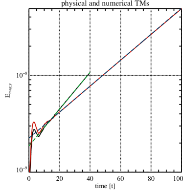
MM
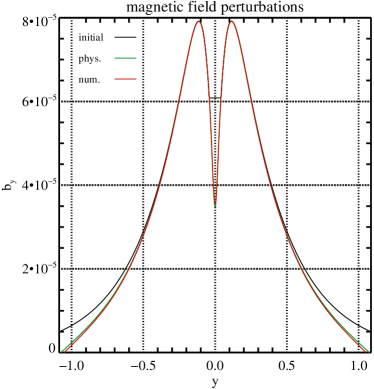
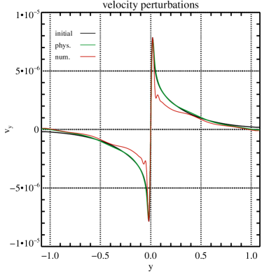
MM

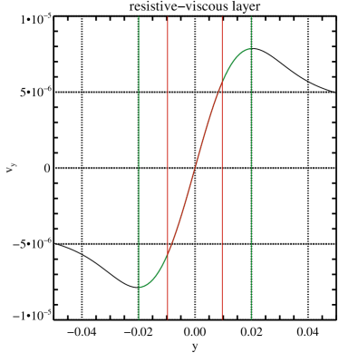
Figure 10: Reference simulation (#Rf, $2048\times 2048$ zones, MP9, HLL Riemann solver) of TM driven by physical resistivity ($\eta=10^{-5}$) and exemplary simulation (#Ex, $384\times 384$ zones, MP5, LF Riemann solver) of TM driven by numerical resistivity (i.e. $\eta=0$). The numerical resistivity is negligible for #Rf ($\eta_{\ast}\ll\eta=10^{-5}$), and has value of $\eta_{\ast}=6.5\times 10^{-6}$ for #Ex (marked by the third rightmost asterisk in Fig. 12). Top left: evolution of the magnetic energy, $\bar{E}_{\mathrm{mag},y}$ (Eq. 101) for simulation #Rf (black line) and #Ex (red line) together with linear fits to the logarithm of $\bar{E}_{\mathrm{mag},y}$ for $t\in[20,40]$ (green and blue dashed lines) from which the instability growth rate can be measured. Top right: initial (black) and evolved profiles of the magnetic field perturbation $b_{1y}$ at $x=-0.5$ in simulation #Rf (at $t=40$; green) and #Ex (at $t=100$; red) normalised to the ratio $\max{|b_{y}(t=0)|}/\max{|b_{y}(t=100)|}$. Bottom left: same as upper right panel, but showing the velocity perturbation $v_{y}$ at $x=0$. The two extrema at $y\approx\pm 0.02$ determine the width of the resistive-viscous layer $L_{\rm RV}$. Bottom right: zoom of the bottom left panel near the current sheet showing the evolved velocity perturbation for simulation #Rf. The two green and two red vertical lines, which are located at $y=\pm L_{\mathrm{RV}}$ and $y=\pm\epsilon_{\mathrm{RV}}$ (Eq. A19), respectively, bracket the resistive viscous layer and the region where the modulus of the dimensionless parameter $\tilde{s}$ (Eq. A28) is smaller than one.

The upper right panel of Fig. 10 shows profiles in $y$ direction of the initial (black) and the evolved (at $t=40$; green) magnetic field perturbations at $x=-0.5$, the latter being normalised to the ratio $\max{|b_{y}(t=0)|}/\max{|b_{y}(t=100)|}$. The corresponding velocity perturbation at $x=0$ (bottom panels) exhibit two pronounced extrema surrounding the magnetic shear layer (marked by the two vertical green lines in the lower right panel, which is a zoom of the lower left panel), which are characteristic of TMs.

To measure the TM growth rate, we compute the evolution with time of the quantity

$$\bar{E}_{\mathrm{mag},y}\equiv\int_{-L_{x}}^{L_{x}}\int_{-a}^{a}\frac{b_{y}^{2}}{2}\ \mathrm{d}x\mathrm{d}y\,,$$ (101)

where the integration is performed only up to $|y|\leq a$ to reduce a potential influence of boundary conditions. After an initial transient lasting up to 20 time units during which the initial perturbation adjusts to the analytic solution, $\bar{E}_{\mathrm{mag},y}(t)$ grows exponentially at a constant rate. Since $b_{y}\propto\exp(\gamma t)$,

$$\frac{1}{2}\ln\left(\bar{E}_{\mathrm{mag},y}\right)=\gamma t+\mathrm{const.},$$ (102)

where the constant depends on the initial perturbation amplitude and the box size. Using the above equation, we compute the instability growth rate by means of a simple linear regression. The black line in the upper left panel of Fig. 10 shows the time evolution of $\bar{E}_{\mathrm{mag},y}$, while the green dashed line is the linear fit according to Eq. (102) -note that both lines are almost indistinguishable after the initial transient time.

To obtain the width of the resistive viscous layer, we plot $v_{y}(x=0,y)$ for every simulation at $t=30$ and measure the locations $L^{+}_{\mathrm{RV}}$ and $L^{-}_{\mathrm{RV}}$ of the two velocity extrema (see vertical green lines in the bottom right panel of Fig. 10). To attribute a measurement error, we note that the extremum can be located anywhere inside of the corresponding computational zone of vertical size $\Delta y$. Thus, the actual location of the extremum is uncertain up to an error $\pm\Delta y/2$, i.e. the layer width is

$$L_{\mathrm{RV}}=\frac{L^{+}_{\mathrm{RV}}-L^{-}_{\mathrm{RV}}}{2}\pm\frac{\Delta y}{2}.$$ (103)

The methodology explained above to measure the growth rate $\gamma$ and the width of the resistive-viscous layer $L_{\mathrm{RV}}$ was applied to all TM simulations discussed below. To understand the dependence of these quantities on the different relevant parameters and to compare with the analytic results, we performed several series of simulations exploring the parameter space in the neighbourhood of the reference model, by varying $\eta$, $\nu$, $b_{0}$ and $k$. Details of these simulations can be found in Appendix A.

The main result extracted from this set of (numerically converged) simulations is the disagreement between the numerically obtained growth rates and the analytic ones given by Eq. (91). The most likely explanation for the discrepancy is that the parameters of our TM simulations are outside of the regime of validity of the analytic results, particularly because of the difficulty to guarantee $L_{\mathrm{R}V}\ll a$. Unfortunately, this means that the analytic expressions (91) and (92) cannot be used to measure numerical resistivity. Thus, we decided to use an empirical approach to the problem.

Using the insight gained from the theoretical work of FKR63, we postulate an ansatz for the dependence of both the TM growth rate and the width of the resistive-viscous layer on the physical parameters, which we then calibrate using the series of numerical simulations mentioned above. The whole procedure is described in detail in Appendix A. The empirical expressions resulting for $k=3$ and $a=0.1$ are

$$\gamma(k=3,a=0.1) =34.56\eta^{4/5}\nu^{-1/5}\left(\frac{b_{0}}{\sqrt{\rho_{0}}}\right)^{2/5},$$ (104)

$$L_{\mathrm{RV}}(k=3,a=0.1) =0.634(\eta\nu)^{1/6}\left(\frac{b_{0}}{\sqrt{\rho_{0}}}\right)^{-1/3}.$$ (105)

Figure 11 shows the TM growth rates (upper panel) and the width of the resistive-viscous layer (lower panel) measured from two series of simulations done with a viscosity $\nu=10^{-4}$ (blue diamonds) and $\nu=10^{-5}$ (red asterisks) for different values of the resistivity. Solid lines represent the empirical expressions given by Eqs. (104) and (105), while the analytic results given by Eq. (91) are plotted with dashed lines in the upper panel of Fig. 11. The discrepancy in the growth rate between analytic and numerical results is obvious, whereas our empirical expression (105) for the width of the resistive-viscous layer is compatible with the analytical one (Eq. 92).

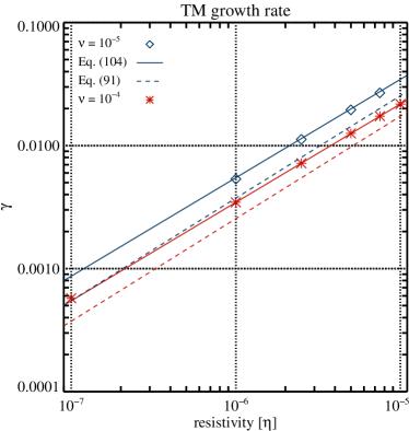
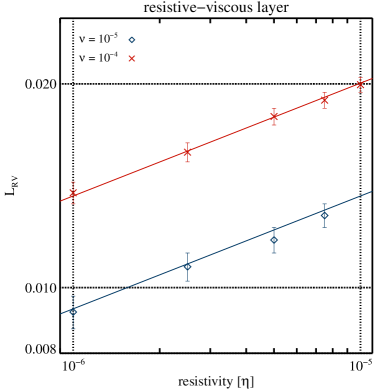
Figure 11: TM growth rate (top) and resistive-viscous layer width (bottom) as a function of resistivity. Blue diamonds and red asterisks denote results of simulations performed with a constant viscosity of $\nu=10^{-5}$ and $\nu=10^{-4}$, respectively. The simulations employed the HLL Riemann solver, MP9, and a grid resolution of $2048\times 2048$ zones. The solid lines are empirical expressions given by Eqs. (104) and (105), respectively. The dashed lines in the upper panel are the analytical predictions given by Eq. (91).

4.3.3 Numerical TM

With the knowledge acquired from the resistive-viscous simulations of the previous section, we can tackle the problem of estimating the numerical resistivity of the code. If we perform a simulation with $\eta=0$, the development of TM signals the presence of a non-zero numerical resistivity $\eta_{\ast}$, because TM are not present in ideal MHD.

For the numerical setup presented in the previous section and for a viscosity $\nu=10^{-4}$, the TM growth rate should be well described by Eq. (104), if $\eta_{\ast}\lesssim 10^{-5}$. In this case, we can determine $\eta_{\ast}$ using the expression

$$\eta_{\ast}=\left(\frac{\gamma(k=3,a=0.1)}{34.56}\right)^{5/4}\nu^{1/4}\left(\frac{\sqrt{\rho_{0}}}{b_{0}}\right)^{1/2},$$ (106)

where we need to measure only the growth rate of the instability, $\gamma$, for a simulation with $k=3$ and $a=0.1$.

Alternatively, one could measure the resistive-viscous layer width (Eq. 105) to obtain $\eta_{\ast}$ from the expression

$$\eta_{\ast}=\left(\frac{L_{\mathrm{RV}}(k=3,a=0.1)}{0.634}\right)^{6}\nu^{-1}\left(\frac{b_{0}}{\sqrt{\rho_{0}}}\right)^{2}.$$ (107)

This method is much less accurate, however, because measuring $L_{\mathrm{RV}}$ from a simulation is prone to rather large relative errors (of the order of $0.1$), and because $\eta_{\ast}\propto L_{\mathrm{RV}}^{6}$.

To compute the numerical resistivity from Eq. (106) we need to know the value of the viscosity $\nu$. However, for a coarse numerical resolution the value of the numerical viscosity can be of the same order. Therefore, we should require $\nu\gg\nu_{\ast}$. Expecting that the numerical resistivity and viscosity are of the same order, we had to choose a value of $\nu$ that is larger than the typical values of both numerical resistivity and numerical viscosity. On the other hand, $\nu$ must not be too large because the growth rate of the instability decreases with increasing $\nu$, i.e. more expensive simulations are required. The size of the resistive-viscous layer also grows with $\nu$ and may become comparable to $a$, thus violating the condition $L_{RV}\ll a$, i.e. Eq. (104) no longer holds. As a compromise, we chose a value of $\nu=10^{-4}$ and performed all simulations with sufficiently high resolution to ensure that $P_{\mathrm{m}}\gg 1$.

Eq. (104) was obtained from numerical simulations in which we removed the background field from the resistive term of the MHD equations (see Eq. 100) to prevent diffusion of the background field. The simulations to be discussed in the remainder of this section did not require this measure, because they were performed without physical resistivity. In spite of this difference, we can still apply the calibration obtained in the former series of simulations, because we find that the results of both series of simulations are consistent (TM develop in both cases, but the background magnetic field dose not diffuse). Hence, numerical resistivity seems to act independently on large scales (diffusion of the background field across the box) and small scales (development of TM). This finding confirms our ansatz, which postulates that the value of numerical resistivity differs for phenomena occurring at different length scales, because $\eta_{\ast}$ depends on the typical length ($\mathcal{L}$) and velocity ($\mathcal{V}$) of the flow.

To determine the dependence of the numerical resistivity on the three Riemann solvers (LF, HLL, HLLD), we performed simulations with the MP5 reconstruction scheme, the RK3 time integrator, a CFL factor of $0.7$, and grids of $128\times 128$ to $1024\times 1024$ zones. The default physical parameters were $a=0.1$, $k=3$, $b_{0}=\rho_{0}=1$, $\nu=10^{-4}$, and $\eta=0$.

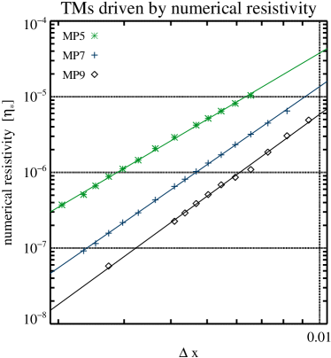
Figure 12: Numerical resistivity of TM simulations performed with $224$ to $1024$ zones (per dimension), the LF Riemann solver, a viscosity $\nu=10^{-4}$, no (physical) resistivity, and the MP5 (green asterisks), MP7 (blue plus signs), and MP9 reconstruction scheme (black diamonds). The straight lines are linear fits to the data.

We find that TM are instigated by numerical resistivity for the LF solver. In the simulations performed with the HLL and HLLD Riemann solvers no TM are observed, i.e. the numerical resistivity resulting from these solvers, although undetermined, must be much less than that of the LF solver. For the latter solver, as expected, the higher the grid resolution the smaller the instability growth rate, i.e. the lower the numerical resistivity (see Fig. 12), since $\gamma\propto\eta^{4/5}$ (Eq. 104). Coarsening the grid resolution, the numerical resistivity eventually becomes so high that the width of the resistive-viscous layer is so large that Eq. (104) is invalid, and we can no longer precisely measure the magnitude of the numerical resistivity. The resolution limit depends on the order of the reconstruction scheme, being $320$, $256$, and $224$ zones per dimension for the MP5, MP7, and MP9 scheme, respectively.

The results of an exemplary simulation (#Ex) without resistivity obtained with MP5 reconstruction scheme on a grid of $384\times 384$ zones are shown in Fig. 10. Like in the reference model #Rf (with $\eta=10^{-5}$; black dashed-dotted line in upper left panel), a TM grows exponentially with time in model #Ex (red dashed-dotted line in the panel), this time being driven by numerical resistivity (in this simulation $\eta_{\ast}=6.5\times 10^{-6}$ marked with the third rightmost asterisk in Fig. 12). The TM induced growth of the magnetic field (upper right panel of Fig. 10) and velocity (bottom left panel) perturbations in model #Ex (without resistivity; red lines) are similar to those in model #Rf (with resistivity; green lines). This comparison clearly demonstrates that the behaviour of the numerical resistivity closely resembles that of (real) physical resistivity.

We anticipate that the main contribution to the numerical resistivity comes from the $y$-direction. All variables exhibit a much stronger variation in $y$-direction than in $x$-direction. Hence, the characteristic length scales in our multi-D ansatz for the numerical resistivity (analogous one to ansatz (24) for numerical shear viscosity), are much larger in $x$-direction than in $y$-direction, $\mathcal{L}_{x}\gg\mathcal{L}_{y}$. More specifically, we can preliminarily estimate that $\mathcal{L}_{x}\propto k^{-1}\propto L_{x}$ and $\mathcal{L}_{y}\lesssim a$. Consequently, the total numerical errors coming from the $x$-direction will be negligible compared to the ones due to the discretisation in $y$, allowing us to use the simpler one-dimensional ansatz in the following. Therefore, in the further discussion of TMs, we will refer to the 1D ansatz for numerical resistivity (Eq. 21) for the sake of simplicity. Furthermore, we will use $\Delta x$ instead of $\Delta y$, since they are equal in our simulations, having in mind, however that the main contribution comes form errors proportional to $(\Delta y/\mathcal{L}_{y})^{r}$. A similar situation occurred in the 2D simulation of sound waves (series #LS6–#LS11 from Tab. 4) in which $(\Delta x/\mathcal{L}_{x})^{r}\gg(\Delta y/\mathcal{L}_{y})^{r}$ and therefore the contribution of the $y$ sweep to the numerical dissipation was negligible and one could equally well use 1D ansatzes for numerical dissipation.

The dependence of the numerical resistivity (which is determined from the measured growth rate of the instability using Eq. 106) on the grid resolution is shown in Fig. 12. The results are fitted with the functions

$$\ln(\gamma) =\alpha_{5}\ln(\Delta x)+c_{5},$$

$$\ln(\gamma) =\alpha_{7}\ln(\Delta x)+c_{7},$$

$$\ln(\gamma) =\alpha_{9}\ln(\Delta x)+c_{9},$$ (108)

where $\alpha_{i}$ and $c_{i}$ are the coefficients of the MP reconstruction scheme of $i-$th order. Their values are (for a CFL factor in the range $0.1$ to $0.7$)

$$\alpha_{5} =2.35\pm 0.02, c_{5}=9.85\pm 0.13,$$

$$\alpha_{7} =2.740\pm 0.015, c_{7}=11.06\pm 0.09,$$

$$\alpha_{9} =2.88\pm 0.05, c_{9}=11.1\pm 0.3.$$ (109)

If the numerical resistivity scales as $\eta_{\ast}\propto\mathcal{V}\mathcal{L}\,(\Delta x/\mathcal{L})^{r}$ as in Eq. (21), one would naively expect that the growth rate scales as $\gamma\propto(\Delta x)^{4r/5}$, i.e. the expected theoretical values should be $\alpha_{5}=4$, $\alpha_{7}=5.6$, and $\alpha_{9}=7.2$, which do not agree with our results. As we explain below, this argumentation is wrong, however, because it fails to account for an (implicit) dependence of the quantities $\mathcal{V}$ and $\mathcal{L}$ on $\eta_{\ast}$.

To explain the apparent considerable reduction of the convergence order $r$ of the MP reconstruction schemes in (109), we need to have a careful look at the ansatz (21) for the numerical resistivity (neglecting the contribution of time integration errors)

$$\eta_{\ast}=\mathfrak{N}_{\eta}^{\Delta x}\mathcal{V}\mathcal{L}\bigg{(}\frac{\Delta x}{\mathcal{L}}\bigg{)}^{r},$$ (110)

where $\mathcal{V}$ and $\mathcal{L}$ are the system’s characteristic speed and length, respectively.

If we were to assume $\mathcal{L}\propto a$ (which is constant), we would obtain $r_{i}=(5/4)\alpha_{i}$. The conceptual mistake we have made here is that $a$ is the correct choice for the characteristic length of the background magnetic field diffusion problem, but not for a TM whose length scale is much smaller than the shear width. It turns out (as we demonstrate below) that the characteristic length of the system is proportional to the width of the resistive-viscous layer, i.e. $\mathcal{L}\propto L_{\mathrm{RV}}$. This seems logical because the current sheet can be described very well neglecting Ohmic dissipation everywhere outside the narrow resistive-viscous layer whose width is $L_{\mathrm{RV}}$ rather than $a$.

The value of $\mathcal{L}$ is somewhat arbitrary, because the boundary of the resistive-viscous layer is (physically) not sharp. We defined its width to be set by the characteristic velocity peaks (see Fig. 8), which is a useful convention for our purpose. In fact, there exists a transition region (marked in shaded yellow in the figure), where the ideal MHD equations can still approximately be applied, although one is already in the non-ideal regime.

For our applications, we found a useful definition based on the fact that resistive and viscous effects are largest in the vicinity of steep gradients of the MHD variables. The (in relative terms) most important gradient is that of the $y$-component of the velocity, which is very large between the two extrema close to the current sheet (see bottom left panel of Fig. 10). Taking into account that $L_{\mathrm{RV}}$ is the half distance between the two extrema, which approximately corresponds to $1/4$ of a wavelength of a sine function, we propose to use as the proper length scale

$$\mathcal{L}=4L_{\mathrm{RV}}.$$ (111)

This choice is consistent with identifying $\mathcal{L}$ with the wavelength in the wave-damping tests. It further suggests that a similar reasoning based on local extrema may lead to the appropriate value in other systems, too. Combining Eqs. (111) and (110), we obtain

$$\eta_{\ast}=\mathfrak{N}_{\eta}^{\Delta x}\mathcal{V}4L_{{\mathrm{RV}}}\bigg{(}\frac{\Delta x}{4L_{{\mathrm{RV}}}}\bigg{)}^{r}.$$ (112)

On the other hand, from Eq. (105), we have

$$L_{{\mathrm{RV}}}(k=3,a=0.1)=0.634\eta_{\ast}^{1/6}\nu^{1/6}\left(\frac{b_{0}}{\sqrt{\rho_{0}}}\right)^{-1/3}.$$ (113)

Note the explicit dependence of Eq. (112) on $L_{{\mathrm{R}V}}$ and of Eq. (113) on $\eta_{\ast}$. This dependence can be easily removed obtaining the expressions

$$\eta_{\ast}= \left[2.536^{(1-r)}\mathfrak{N}_{\eta}^{\Delta x}\mathcal{V}\nu^{(1-r)/6}\left(\frac{b_{0}}{\sqrt{\rho_{0}}}\right)^{-(1-r)/3}(\Delta x)^{r}\right]^{6/(5+r)}$$ (114)

$$L_{{\mathrm{RV}}}= \left[\frac{0.2596}{4^{r}}\nu\left(\frac{b_{0}}{\sqrt{\rho_{0}}}\right)^{-2}\mathfrak{N}_{\eta}^{\Delta x}\mathcal{V}(\Delta x)^{r}\right]^{1/(5+r)}\,,$$ (115)

which are valid only for $a=0.1$ and $k=3$, and give the true dependence of $\eta_{\ast}$ and $L_{{\mathrm{RV}}}$ on the grid resolution. Consequently, the TM growth rate is expected to depend on $\Delta x$ with an exponent $\alpha_{i}=24r/[5(5+r)]$, which allows us to compute the order of convergence from the numerical values $\alpha_{i}$ as

$$r=\frac{25\alpha_{i}}{24-5\alpha_{i}}.$$ (116)

Similarly, Eq. (114) can be used to compute $\mathfrak{N}_{\eta}^{\Delta x}$ resorting to the coefficient $c_{i}$ from the fit to the growth rate and identifying $\mathcal{V}$ as the magnetosonic speed, i.e. $\mathcal{V}=c_{ms}\approx 1.63$ in this case ($\theta=\pi/2$ in Eq. 47).

Reconstruction	$\mathfrak{N}_{\eta}^{\Delta x}$	$r$
MP5	$16\pm 5$	$4.81\pm 0.09$
MP7	$142\pm 33$	$6.65\pm 0.08$
MP9	$\ \ 170\pm 220$	$7.6\pm 0.6$

Table 5: Resistivity coefficient $\mathfrak{N}_{\eta}^{\Delta x}$ (for the definition see Eq. (21)) and reconstruction scheme order $r$ (Eq. (116)) determined from TM simulations performed with the LF Riemann solver (see also Fig. 15).

In Table 5, we list the values of $\mathfrak{N}_{\eta}^{\Delta x}$ and $r$ computed with the procedure outlined above. The MP5 and MP7 schemes are almost 5th and 7th order accurate, whereas the MP9 scheme performs below the theoretical expectation. In other words, the higher the order of the reconstruction scheme, the higher the reduction of the convergence order. A possible explanation of this fact is the following. The function $\textsl{v}_{y}$ is proportional to $y^{-1}$ for $|y|\ll a$, i.e., outside of the resistive-viscous layer (see the discussion in Appendix A, in particular Eq. A6 and Fig. 17). For this reason all the derivatives of $\textsl{v}_{y}$ in the $y-$direction diverge. Thus, the neglected higher order terms of the Taylor expansion in the reconstruction of $\textsl{v}_{y}$ for $y\approx 0$ can actually be dominant. Taking this into consideration, it is rather more surprising that the MP5 and MP7 schemes almost achieve their theoretical order of accuracy than the fact that the MP9 scheme performed below the theoretical expectation.

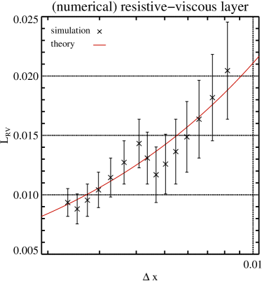
Figure 13: Width of the resistive-viscous layer as a function of $\Delta x$ (which is proportional to the value of the numerical resistivity) in simulations of TM driven by numerical resistivity. Black crosses depict measured values obtained in simulations with MP7. The red curve shows the expected layer width (Eq. 115), given the parameters for the numerical resistivity determined from the measured growth rate.

According to Fig. 13, the values of $L_{{\mathrm{R}V}}$ measured directly from the numerical simulations (see previous section) agree well with those computed with Eq. (115), where the values of $r$ and $\mathfrak{N}_{\eta}^{\Delta x}$ needed in this equation are extracted from the growth rate using Eqs. (109) and (116). This result shows that our assumptions are correct, which is far from being obvious, because we assumed that (i) numerical errors can be called “numerical resistivity”, (ii) this numerical resistivity can be treated as normal physical resistivity, and (iii) the same equations can be used to determine its magnitude or predict its influence on the system. Moreover, we also had to make use of ansatz (21) for the numerical resistivity.

To test whether the magnetosonic speed is indeed the characteristic velocity of our TM setup, as expected from the arguments given in the discussion of the wave damping simulations, we ran several simulations with the same setup, but varying the fast magnetosonic speed from $c_{\mathrm{ms}}\approx 1$ to $\approx 39$. This was achieved by changing the background pressure from $0.01$ to $900$, keeping $b_{0}=\rho_{0}=1$. The upper panel of Fig. 14 shows that the numerical resistivity increases with $c_{\mathrm{ms}}$.

Different from the wave damping tests, it is not straightforward, however, to compute the fast magnetosonic speed, because in TM simulations the perturbed fluid makes a “U-turn” in the vicinity of the magnetic shear layer (i.e. for $|y/a|\ll 1$). Therefore, determining the “correct” values of $\theta$ (which changes from $0$ to $\pi/2$) and the background magnetic field strength (which changes from $1$ for $|y/a|\gg 1$ to $0$ for $|y/a|\approx 0$) is very error-prone. That is why we introduced ansatzes (17), (20), and (21) to have a simple way of estimating the code’s numerical dissipation. Consequently, we took the maximum possible magnetosonic speed (obtained for $\cos\theta=0$; Eq. 47) in our previous analysis, i.e.

$$c_{\mathrm{ms}}=\sqrt{c_{\mathrm{A}}^{2}+c_{\mathrm{s}}^{2}}.$$ (117)

and put $c_{\mathrm{A}}=1$, which is well motivated by practical purposes (i.e. to keep the ansatzes as simple as possible). However, in the current analysis (simulations presented in Fig. 14), we obtained a better fit with respect to $c_{\rm ms}$ with $c_{\mathrm{A}}=0.76$, which corresponds to the Alfvén speed at a distance $y=a$, i.e.

$$c_{\mathrm{ms}}=\sqrt{5/3p_{0}+0.76^{2}}.$$ (118)

We note that the precise choice of $c_{\mathrm{A}}$ is irrelevant in the high plasma $\beta$ regime, while it only slightly affects the quality of the fits in the low plasma $\beta$ regime (where the parameter $\beta\equiv b_{0}^{2}/(2p_{0})$) .

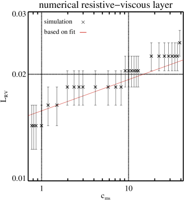
Figure 14: Upper panel: Numerical resistivity in TM simulations performed with MP5 on a grid of $512\times 512$ zones as a function of the fast magnetosonic speed $c_{\mathrm{ms}}$ (Eq. 118), which was changed varying $p_{0}$ but keeping $b_{0}$ and $\rho_{0}$ constant. The black curve is a fit to the simulation data. Bottom panel: Width of the resistive-viscous shear layer (black crosses) as a function of $c_{\mathrm{ms}}$ for the simulations shown in the upper panel. The red curve gives the predicted width of the resistive-viscous layer based on the fit in the upper panel.

From the measured growth-rates $\gamma$, we determined the numerical resistivity in each simulation ($\eta_{\ast}\propto\gamma^{5/4}$), and fitted the results with

$$\ln(\eta_{\ast})=s\ln(c_{\mathrm{ms}})+d$$ (119)

obtaining

$$s =0.524\pm 0.002,$$

$$d =-12.9\pm 0.5.$$ (120)

From Eq. (114) and Eq. (104), we find that

$$\eta_{\ast}\propto\mathcal{V}^{6/(5+r)}\,,$$ (121)

and putting $\mathcal{V}=c_{\mathrm{ms}}$ in Eq. (121), we finally obtain

$$s=\frac{6}{5+r}.$$ (122)

For MP5 reconstruction ($r_{\rm th}=5$), the expected value is $s=0.6$, which is close to the measured one. Using $s$ from Eq. (120), we determine the reconstruction scheme order to be $r=6.45\pm 0.05$, which is neither equal to $5$ within the errors nor consistent with the value $r=4.81\pm 0.09$ from Tab. 5. This discrepancy should not concern us, however, because we included only statistical errors in the measurement errors from the linear fit neglecting other errors, e.g. those originating from estimating the fast magnetosonic speed (which changes from zone to zone in the simulation). This implies that this way of determining the order of the reconstruction scheme is much less reliable than from the resolution studies.

In the bottom panel of Fig. 14, we show the measured width of the resistive-viscous layer and its value (red curve) predicted from the fit Eq. (119). Using the values of $s$ and $d$ in Eq. (120) we determined $r$ and $\mathfrak{N}_{\eta}^{\Delta x}$, which we then inserted into Eq. (115). This methodology demonstrates that our model is self-consistent, since the width of the resistive-viscous layer does depend on $c_{\rm ms}$ as expected.

At the beginning of this section we made the assumption that the numerical resistivity is not changing the background magnetic profile, but affects only the flow in the resistive-viscous layer, where TM grow. All consistency checks performed in this section seem to indicate that our assumption is correct. As a confirmation, we checked that in none of the simulations there has been a significant modification of the background profile. This finding differs from the one obtained in the simulations with physical resistivity but without removing the background field from the induction equation (100). In those simulations, the background field started to diffuse during the simulations (which was the reason why we modified the induction equation (Eq. 100) in the first place).

Finally, in Fig. 15, we present a comparison of the expected numerical dissipation in simulations of TM and magnetosonic wave damping based on our ansatz (see Eqs. 17, 20, and 21) and the estimators from Tables 1 and 5. For the simulations, we set the characteristic velocities and lengths equal to one, i.e. $\mathcal{V}=\mathcal{L}=1$. The box length is set to 1 too, hence “resolution” in the abscissa of Fig. 15 refers to the number of zones per characteristic length. As we can see, the expected numerical dissipation based on calibration with the help of both types of simulations (MS waves and TM) is similar. This is an indication that our approach is presumably universal, and it makes us confident that it can be used to estimate dissipation coefficients for other flows.

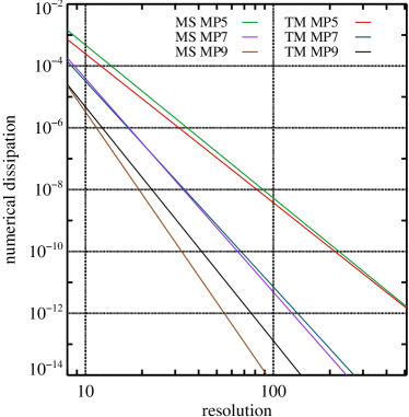
Figure 15: Comparison of the numerical dissipation of Aenus when simulating magnetosonic waves (MS) and tearing modes (TM) with different reconstruction schemes (MP5, MP7, and MP9) and RK3. The numerical dissipation is given by $(4/3)\nu_{\ast}+\xi_{\ast}+\eta_{\ast}/(1+c_{\mathrm{s}}^{2}/c_{\mathrm{A}}^{2})$ in the former case and by $\eta_{\ast}$ in the latter case. For the wave simulations, we found that $\eta_{\ast}/(1+c_{\mathrm{s}}^{2}/c_{\mathrm{A}}^{2})\ll(4/3)\nu_{\ast}+\xi_{\ast}$ (see Sec. 4.1.3). For the wave problem both the HLL and the LF Riemann solver result in a very similar amount of dissipation, whereas for the TM simulations $\eta_{\ast}(\mathrm{HLL})\ll\eta_{\ast}(\mathrm{LF})$. The CFL factor was chosen such that time integration errors were negligible. The results are renormalised by setting the characteristic velocity and length equal to one, i.e. $\mathcal{V}=\mathcal{L}=1$.

5 CASE STUDY: MAGNETOROTATIONAL INSTABILITY

In the previous section, we present a methodology which allows us to estimate the numerical viscosity (bulk and shear) and resistivity of a code. It also serves to determine the characteristic velocity, $\mathcal{V}$, relevant for the numerical dissipation coefficients. We applied this methodology to the AENUS code for different numerical schemes. Using the ansatzes Eqs. (17), (20) and (21) and the numerical dissipation coefficients given by Tables 3 (for shear and bulk viscosity coefficients) and 5 (for resistivity coefficients), it is possible to determine the numerical resolution, $\Delta x$, needed to perform a numerical simulation with a numerical viscosity and resistivity lower than a given threshold. This allows us to estimate the computational resources needed for a particular application and helps us to choose the numerical scheme that minimises the computational cost. To show the feasibility and the usefulness of this analysis, we present here the estimates for a particular application of AENUS to simulations of the MRI.

The MRI (Velikhov, 1959; Chandrasekhar, 1960) is an instability which can develop in a differentially rotating fluid in the presence of a magnetic field. In the case of an homogeneous vertical magnetic field the MRI develops non-linear channel flows which are then disrupted by parasitic instabilities (Goodman & Xu, 1994; Pessah & Goodman, 2009) into a turbulent flow. The instability has been proposed as the main driver of accretion in accretion disks (Balbus & Hawley, 1991) and may play an important role in the amplification of magnetic field during the collapse of stellar cores (Akiyama et al., 2003). There are a number of MHD simulations devoted to the study of the MRI in local box simulations (see e.g. Obergaulinger et al., 2009; Rembiasz et al., 2016a, b) in which we can aim to resolve numerically the magnetised flow with minimal numerical viscosity and resistivity. The main difficulty of those simulations is that the characteristic length scale relevant for the growth of the MRI channel modes and its termination due to parasitic instabilities (Kelvin-Helmholtz vortices) is very small ($\mathcal{L}\sim 100$ m) compared to the size of the system ($\sim 10$ km) when realistic conditions are considered (see Obergaulinger et al., 2009, for a discusion). Here we show, as an example, how one can estimate the resolution requirement and computational cost for the numerical simulations presented in Rembiasz et al. (2016b).

In the typical setup of Rembiasz et al. (2016b) the box size is $2{\rm\,km}\times 2{\rm\,km}\times 0.666{\rm\,km}$ or $2{\rm\,km}\times 8{\rm\,km}\times 2{\rm\,km}$ (radial, azimuthal and vertical extension) and channel modes develop with a size of $\lambda_{\rm MRI}=0.666$ km in the vertical direction (one or three channel modes fit in the vertical direction, depending on the box size). The characteristic length is set by the width of the channel mode, i.e. $\mathcal{L}=\lambda_{\rm MRI}$. The characteristic speed may be chosen among the fast magnetosonic speed ($c_{\rm ms}=3\times 10^{9}$ cm s^-1), the Alfvén speed, ($c_{\rm A}=7.8\times 10^{7}$ cm s^-1), or the flow velocity ($v_{\rm flow}=2.4\times 10^{9}$ cm s^-1). To make a conservative estimate we take the largest of the three, i.e. $\mathcal{V}=3\times 10^{9}$ cm s^-1. The goal of Rembiasz et al. (2016b) was to run the simulations with numerical viscosities and resistivities below a value of $7.48\times 10^{8}$ cm² s^-1 (according to estimates of Guilet et al., 2015, (physical) viscosity due to neutrinos can vary from $10^{9}\text{--}10^{12}$ cm² s^-1 inside of a proto-neutron star). They estimated that in that regime the Reynolds numbers are above $\sim 100$, which would be sufficient to have convergent results for the growth of the channel flows up to the termination due to parasitic instabilities. The post-termination evolution of the generated turbulent flow would have probably required more stringent resolutions, but this was not the aim of Rembiasz et al. (2016b).

Figure 16 shows the estimated numerical viscosities and resistivities of the AENUS code according to the measurements of the present work rescaled to the simulations of Rembiasz et al. (2016b) for an HLLD solver and three different reconstruction schemes (MP5, MP7 and MP9). According to the figure, it is sufficient to perform simulations with $10$, $14$, and $28$ zones per $\mathcal{L}$ to reach the accuracy goal for MP9, MP7, and MP5, respectively. This result demonstrates the advantage of using ultra-high order schemes (MP9) in simulations of smooth flows

Once the numerical resolution is known, it is possible to estimate the computational cost of a given simulation. As an example, we consider our smallest simulation box ($2{\rm\,km}\times 2{\rm\,km}\times 0.666{\rm\,km}$), a typical simulation period of $12$ ms duration, and a CFL factor of $0.7$. AENUS performs on the SuperMUC supercomputer (www.lrz.de) typically at $0.15$ ms/iteration/zone. The upper abscissa of Fig. 16 shows the resulting total CPU time for this setup. To reach the accuracy goal, we estimate that we need at least $15$, $60$, and $842$ CPU hrs for MP9, MP7, and MP5, respectively. Even if MP9 suffers of a slight computational overhead in comparison to MP7 and MP5, due to the larger size of the numerical stencil, our analysis shows that it pays off to perform simulations with MP9. Indeed, Rembiasz et al. (2016b) performed their simulations with resolutions ranging from $20$ to $134$ zones per $\lambda_{\rm MRI}$ and showed convergence of the results.

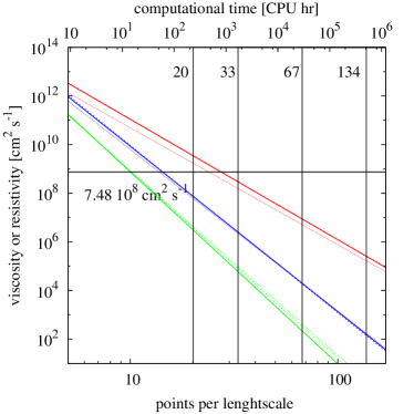
Figure 16: Estimation of the numerical shear viscosity (solid lines), bulk viscosity (dashed lines), and resistivity (dotted lines) for the MRI simulations of Rembiasz et al. (2016b) for different numbers of grid points per length scale ($\Delta x/\mathcal{L}$; lower abscissa). Results are shown for three different reconstruction schemes: MP5 (red), MP7 (blue), and MP9 (green). Vertical black lines show the resolution used in that work. The horizontal black line shows the viscosity and resistivity goal, below which the Reynolds numbers exceed a value of $\sim 100$. The upper abscissa gives an estimate of the corresponding computational cost of a $12$ ms simulation with AENUS for the smallest box size ($2{\rm\,km}\times 2{\rm\,km}\times 0.666{\rm\,km}$).

6 SUMMARY AND CONCLUSIONS

We have presented a reliable methodology to measure the numerical shear and bulk viscosity, and the resistivity of Eulerian finite volume MHD codes by means of a simple ansatz for each of these numerical effects, which are inevitably present in any such code. We have postulated that the amount of numerical dissipation depends on the characteristic length and velocity of the system under consideration, the numerical resolution, and some free parameters which have to be calibrated depending on the numerical scheme in use. Hence, our ansatz for each of the three numerical effects consists of two additive terms describing the contribution of spatial and temporal discretisation errors, which both depend on the characteristic length and velocity of the system, and on the grid resolution and the size of the time step, respectively.

We performed the parameter calibration by means of a set of test simulations using the Aenus code. However, because the procedure is not restricted to this code, we provide potential users of our methodology with the detailed results of our test suite at http://www.uv.es/camap/tmweb/Web_tm.html. These data should help to measure the dissipation coefficients of other Eulerian finite volume MHD codes.

Firstly, we have considered three wave damping tests from which one can directly extract a linear combination of the numerical resistivity, and the numerical shear and bulk viscosities. These simulations allowed us to estimate the latter two quantities accurately. However, we failed to obtain a physically sound value of the numerical resistivity, because it is much smaller than that of the numerical viscosity of Aenus, i.e. our estimate of the numerical resistivity is dominated by systematic errors.

Nevertheless, the wave damping simulations confirm the appropriateness of our ansatz for the numerical shear and bulk viscosity, and the resistivity. In almost all simulations performed by us, the spatial reconstruction schemes and the RK time integrators have the theoretically expected order of accuracy. We also find that in simulations of sound waves, Alfvén, waves, and fast magnetosonic waves the characteristic length and velocity of the system are always the wavelength of the wave and the fast magnetosonic speed (which reduces to the sound speed in the case of sound waves), respectively. Because the value of the numerical resistivity is substantially lower than that of the numerical viscosity in the wave damping tests (see above), the numerical magnetic Prandtl number $P_{\mathrm{m}\ast}\equiv\nu_{\ast}/\eta_{\ast}$ is not close to $1$, as it is commonly suspected among practitioners in the field.

Secondly, we have performed TM simulations since the wave damping ones were hardly useful to asses the value of the numerical resistivity. By measuring the growth rate of the TM instability and fixing the value of the physical viscosity, we have been able to estimate the numerical resistivity of Aenus. Moreover, from the estimated value of the numerical resistivity, we could correctly predict the expected width of the resistive viscous layer. This indicates that our method is (self-)consistent. A cautionary note must be added here. In order to obtain reliable estimates of the numerical resistivity in TM simulations it is necessary to employ spatial reconstruction schemes of order $r\geq 5$. Extensive numerical experience (Rembiasz, 2013) shows that the TM setup employed here becomes numerically unstable for lower order reconstruction schemes in the resolution range considered by us, i.e.  it was difficult to maintain a magnetohydrodynamical equilibrium of the background flow for tests in which less than a fifth order spatial reconstruction scheme was employed.

Comparing the expected numerical dissipation in simulations of magnetosonic wave damping and TM, we find that the expected numerical dissipation based on a calibration with the help of both types of simulations is similar. This indicates that our approach is supposedly universal, which gives us confidence that it is also applicable to estimate the dissipation coefficients for different flow regimes and numerical setups. For illustration of our approach in an astrophysical context, we have estimated in Sec. 5 the numerical viscosities and resistivity for the MRI models of Rembiasz et al. (2016b), which in turn have allowed us to obtain a reliable estimate of the computational needs in terms of numerical resolution and computational time for these particular simulations.

We have found that the high orders of convergence of the MP reconstruction schemes obtained in the wave damping tests are retained in the 2D simulations of sound waves and TMs. This is a remarkable result, because our approach is based on several (one per dimension) independent one-dimensional reconstruction steps instead of a genuinely multi-D reconstruction algorithm as proposed by, e.g. Colella et al. (2011); McCorquodale & Colella (2011); Zhang et al. (2011); Buchmüller & Helzel (2014). In general, such a simplification may introduce additional numerical errors, thus degrading the order of accuracy of multi-D simulations to second order, i.e. well below that of 1D ones.

However, our 2D simulations do not suffer from this degradation. This may be the result of our somewhat simple tests, i.e. in the TM case, the derivatives in the $y$-direction dominate over the ones in the $x$-direction, and in 2D simulations of sound waves, we consider small sinusoidal perturbations of the background. One should not expect this behaviour to hold in a general case of a non-linear multi-D problem. Exploring this topic is beyond the scope of this work though.

It is important to note that in our ansatz there is a single length scale $\mathcal{L}$ for which the dissipation coefficients are estimated. If applied to systems in which dissipation occurs at multiple length scales (e.g. turbulence), then the interpretation of our ansatz is a measurement of the dissipation coefficients at each length scale, which may give rise to different values of these coefficients. Indeed, we observe this effect in our TM simulations, if the background magnetic field is not eliminated from the induction equation. If not eliminated, we have dissipation occurring both in the resistive-viscous layer (of size $L_{\rm RV}$) and within the background shear profile (of size $a>>L_{\rm RV}$) at the same time. This scale-dependent definition of the dissipation coefficients is similar to that used in large eddy simulations of anisotropic weakly compressible turbulence (see e.g. Fureby & Grinstein, 1999; Zhou et al., 2014; Radice, Couch, & Ott, 2015). Alternatively, we could have formulated our ansatz equivalently in terms of scale-independent hyperviscosity and hyperresistivity coefficients. This formulation has the disadvantage of not having physical counterparts for the purely numerical hyperdissipation coefficients but, on the other hand, it allows to interpret the high-order derivative terms appearing in the Taylor expansion of the space and time derivatives (see Eq. 10).

Using our ansatz may not always be straightforward, since it requires identifying the relevant characteristic velocity $\mathcal{V}$ and length $\mathcal{L}$, of the system. As for the former, we have shown that in all our tests (wave damping and TM) without background flow, the characteristic velocity is equal to the fast magnetosonic speed. In the wave-damping tests with a non-zero background velocity (see Sec. 4.1.5), we have found that the characteristic velocity depends on the direction of the wave propagation relative to the direction of the background flow. However, one can easily obtain an estimate for the upper limit of the characteristic velocity, i.e. for the sum of the moduli of the background velocity and the fast magnetosonic speed. The determination of the characteristic length, $\mathcal{L}$, of the system can be tricky and requires a good understanding of the simulated system. For example, in the case of the TM simulations, the first “natural candidate” for $\mathcal{L}$ seems to be the width of the magnetic shear layer, $a$, (Eq. 76), but it turns out to be the width of the resistive-viscous layer, $L_{\rm RV}$ (Eq. 105).

Even though all our test were performed in boxes with uniform grid resolutions, our results can be translated to adaptive mesh refinements (AMR) codes that refine the grid where the flow develops small-scale structures. A natural way of using our ansatzes in AMR simulations would be to apply it at each refinement level separately, i.e. to compute the numerical dissipation coefficients (21) based on the refined grid width. Numerical viscosity and resistivity then quite obviously are position-dependent. This is, however, not a unique feature of AMR simulations because, in general, numerical viscosity and resistivity are local quantities because they depend on the characteristic velocity and length scale that may vary strongly throughout the simulation domain.

Finally, we note that in the (astro-)physics literature hydrodynamic and magnetohydrodynamic simulations are often categorised by the numerical Reynolds numbers

$$R_{{\rm e}\ast}=\frac{VL}{\nu_{\ast}}\qquad,\qquad R_{{\rm m}\ast}=\frac{VL}{\eta_{\ast}},$$ (123)

where $L$ and $V$ are the typical length and typical velocity of the system, respectively. However, often both quantities are subjectively chosen. In other words, the assumed typical length and velocity of the system are not the values obtained after a thorough calibration analysis as we have conducted it here. Indeed, in general, $L\neq\mathcal{L}$ and $V\neq\mathcal{V}$, i.e. the typical values (chosen by the respective author) are not equal to the characteristic values, which are uniquely set by the physics and numerics of a given simulation. Hence, the Reynolds numbers commonly estimated can vary by a few orders of magnitude for the same physical system and numerical setup across the literature. For this reason, the typical values of the numerical Reynolds number seldomly are a useful quantity to cross-compare different numerical models. However, once the numerical viscosity and resistivity are measured (as we propose it in this paper), one can easily express simulation results in terms of numerical hydrodynamic and magnetohydrodynamic Reynolds numbers, in as much as the proper characteristic length and velocity of the system have been identified. Because this is not a common practice in the community, we conclude that the use of numerical Reynolds numbers more often obscures than reveals the true nature of numerical viscosity and resistivity.

Appendix A TEARING MODE GROWTH RATE

In Appedix A.1, we present an analytical derivation of the TM growth rate in resistive MHD, and we briefly discuss a generalisation of these results to resistive-viscous MHD, which was already done by FKR63.

In Appendix A.2, we postulate empirical equations for the TM growth rate in resistive-viscous MHD and calibrate these rates with the help of numerical simulations.

A.1 Analytical Approach

In their analytical study of the TM instability, FKR63 considered the effects of various physical factors, like a position dependent background density, temperature, and resistivity. We will restrict ourselves to a much simpler system, yet demonstrating the key features of the TM instability. Our presentation is greatly inspired by the excellent discussion of this topic in Goedbloed et al. (2010). We also recommend Schnack (2009) for a concise introduction to the TM instability.

A.1.1 General Case

We consider perturbations of the system described in Sec. 4.3.1 whose wavelength in $x$ direction is comparable to the shear width, i.e. $k\lesssim a^{-1}$ (Eq. 84). Note that one only needs to solve Eqs. (77) and (78) for $\textsl{v}_{y}$ and $b_{1y}$, respectively, while the other perturbation components can be easily determined from conditions (79) and (80). For the WKB ansatz (Eqs. 81 and 82) to be justified, condition (83) must be satisfied.

Inserting the WKB ansatz into Eqs. (77) and (78) and taking the curl of the latter equation to eliminate the pressure, the $y$ component of the induction equation and the derivative $\partial_{x}$ of the $z$ component of the equation of motion read

$$\gamma b_{1y}= [\nabla\times({\bf v}\times{\bf b_{0}})]_{y}+\eta(-k^{2}+\partial^{2}_{y})b_{1y},$$ (A1)

$$\gamma\rho_{0}(-k^{2}+\partial^{2}_{y})\textsl{v}_{y}= \partial_{x}\{\nabla\times[(\nabla\times{\bf b_{1}})\times{\bf b_{0}}+(\nabla\times{\bf b_{0}})\times{\bf b_{1}}+\rho_{0}\nu\nabla^{2}{\bf v}]\}_{z}.$$ (A2)

After some algebra we arrive at

$$\gamma b_{1y}= ik\textsl{v}_{y}b_{0x}+\eta(-k^{2}+\partial^{2}_{y})b_{1y},$$ (A3)

$$\gamma\rho_{0}(-k^{2}+\partial^{2}_{y})\textsl{v}_{y}= \rho_{0}\nu(k^{4}-2k^{2}\partial_{x}^{2}+\partial_{x}^{4})\textsl{v}_{y}+ik[-b_{1y}\partial_{y}^{2}b_{0x}+b_{0x}(-k^{2}+\partial_{y}^{2})b_{1y}].$$ (A4)

Because this system cannot be integrated analytically, FKR63 used the BLA method (see Sect. 4.3.1). They divided the domain into two regions, an outer one ($-L_{y}\leq y<-y_{\epsilon}$ and $y_{\epsilon}<y\leq L_{y}$, where $y_{\epsilon}$ is a small positive constant such that $y_{\epsilon}\ll a$) in which dissipative effects can be neglected, and an inner layer ($-y_{\epsilon}<y<y_{\epsilon}$) in which resistivity (and viscosity) are important (see Fig. 8). The complete solution is determined by an interplay between both regions: resistivity acts in the inner region, but the rate at which magnetic field lines are reconnected also depends on the rate at which the field can be advected into and out of the inner region. Hence, the growth rate can be quite different for field profiles that are the same close to $y=0$, but differ elsewhere.

Outer Layer

Condition (83) implies that there are negligible field gradients in the outer regions ($|y|>y_{\epsilon}$), i.e. resistive processes are slow there compared to the growth of TMs. On the other hand, $\gamma\gg a^{-2}\eta\sim k^{2}\eta$ (the second relation follows from assumption 84). Hence, to solve Eqs. (A3) and (A4) in the outer region the resistivity term in the induction equation (A3) can be neglected, i.e.

$$ik\textsl{v}_{y}b_{0x}=\gamma b_{1y}\ .$$ (A5)

Furthermore, from the second part of condition (83), we have $\gamma\ll c_{\mathrm{A}}/L_{y}\sim c_{\mathrm{A}}k$. This inequality together with Eq. (A5) imply that terms proportional to velocity (gradients) in Eq. (A4) are negligible, i.e. $|\gamma\rho_{0}k^{2}\textsl{v}_{y}|\ll|ik^{3}b_{0x}b_{1y}|$. Hence, TMs evolve so slowly that the plasma inertia (terms containing $\rho_{0}\textsl{v}_{y}$ in Eq. A4) can be neglected on the ideal MHD time scale, and Eqs. (A3) and (A4) simplify to

$$ik\textsl{v}_{y} =\frac{\gamma b_{1y}}{b_{0x}},$$ (A6)

$$ik[-b_{1y}\partial_{y}^{2}b_{0x}+b_{0x}(-k^{2}+\partial_{y}^{2})b_{1y}] =0.$$ (A7)

in the outer layers. So far, we have not yet made any assumption concerning the background magnetic field. For $b_{0x}(y)=b_{0}\tanh(y/a)$, the solution of Eq. (A7) reads

$$b_{1y}(y)=b_{1}\left(\frac{1+\tanh(y/a)}{1-\tanh(y/a)}\right)^{a\,k/2}\frac{\tanh(y/a)-ak}{\Gamma(2-ak)},$$ (A8)

where $b_{1}$ is a constant (initial perturbation amplitude) and $\Gamma$ denotes the Euler gamma function. The velocity perturbations can be easily determined combining Eqs. (A6) and (A8):

$$\textsl{v}_{1y}(y)=\frac{\gamma b_{1}}{ikb_{0}}\left(\frac{1+\tanh(y/a)}{1-\tanh(y/a)}\right)^{a\,k/2}\frac{\tanh(y/a)-ak}{\Gamma(2-ak)\tanh(y/a)}.$$ (A9)

Note that Eq. (A6) has a singularity for $|y/a|\rightarrow 0$, i.e. for $|b_{0x}|\rightarrow 0$, which is removed (i.e. smearded out) by resistivity in the inner region.

Inner Layer

Resistive (and viscous) terms can no longer be neglected in the inner layer ($|y|<y_{\epsilon}$), and we have to solve Eqs. (A3) and (A4) simultaneously. Because in the inner region $|y/a|\ll 1$, we can approximate the background magnetic field (Eq. 76) as $b_{0x}(y)\approx b_{0}y/a$ (Eq. 85). In the inner region, perturbations in both velocity and magnetic field vary more strongly in the $y$ direction than in the $x$ direction, i.e. $|k^{2}\textsl{v}_{y}|\ll|\partial_{y}^{2}\textsl{v}_{y}|$ and $|k^{2}b_{1y}|\ll|\partial_{y}^{2}b_{1y}|$. Therefore, we can neglect the terms proportional to $k^{2}$ in Eqs. (A3) and (A4), and we obtain

$$\gamma b_{1y} =ik\textsl{v}_{y}b_{0}a^{-1}y+\eta\partial^{2}_{y}b_{1y},$$ (A10)

$$\gamma\rho_{0}\partial^{2}_{y}\textsl{v}_{y} =\rho_{0}\nu(-2k^{2}\partial_{y}^{2}+\partial_{y}^{4})\textsl{v}_{y}+ikb_{0}a^{-1}y\partial_{y}^{2}b_{1y},$$ (A11)

where we used also Eq. (85). Combining both equations into a single one by eliminating terms that contain $b_{1y}$, we arrive at a sixth-order ordinary differential equation (ODE) for $\textsl{v}_{y}$ that reads

$$\textsl{v}_{y}^{(6)}[\nu\eta y^{2}]+\textsl{v}_{y}^{(5)}[-2\nu\eta y]+\textsl{v}_{y}^{(4)}[-(\gamma(\eta+\nu)+2\nu\eta k^{2})y^{2}+2\nu\eta]+$$

$$\textsl{v}_{y}^{(3)}[2\eta(\gamma+2\nu k^{2})y]+\textsl{v}_{y}^{(2)}[k^{2}a^{-2}c_{\rm A}^{2}y^{4}+\gamma(\gamma+2\nu k^{2})y^{2}-2\eta(\gamma+2\nu k^{2})]+\textsl{v}_{y}^{(1)}[2k^{2}a^{-2}c_{\rm A}^{2}y^{3}]=0,$$ (A12)

where $c_{\rm A}^{2}\equiv b_{0}^{2}/\rho_{0}$ and $\textsl{v}_{y}^{(n)}\equiv\partial_{y}^{n}\textsl{v}_{y}$. This equation cannot be integrated analytically, i.e. some further approximations are necessary.

In the inner layer, but sufficiently far away from $y=0$, velocity perturbations will have a solution of type $\textsl{v}_{y}\propto y^{-1}$, i.e. the terms with the highest order derivatives of $\textsl{v}_{y}$ dominate the solution of (A12). Thus, we proceed neglecting lower order derivatives in (A12). Because the two terms with the highest order derivatives ($\partial_{y}^{6}\textsl{v}_{y}$ and $\partial_{y}^{5}\textsl{v}_{y}$) depend on viscosity, we consider Eq. (A12) for two limiting cases, namely in the viscous and the inviscid regime.

A.1.2 Inviscid Case

In the inviscid case ($\nu=0$), Eq. (A12) reduces to a fourth order differential equation that is still too complicated to be solved analytically. Therefore, we follow FKR63 and use their constant $\psi$ approximation.

FKR63 noted that the function $\textsl{v}_{y}$ becomes singular in ideal MHD because $\textsl{v}_{y}\propto y^{-1}$ for $y\rightarrow 0$ (see Eq. A6), i.e. $\textsl{v}_{y}$ varies strongly in the limit of small resistivity. Resistivity regularises this ill-behaved solution. The function $b_{1y}$ varies less for $|y/a|\approx 0$ and can be approximated by a constant $b_{1y}(y)\approx b_{1y}(0)$. With this approximation, Eqs. (A10) and (A11) reduce to

$$\gamma\eta\rho_{0}\partial_{y}^{2}\textsl{v}_{y}-k^{2}a^{-2}b_{0}^{2}\textsl{v}_{y}y^{2} =ik\gamma b_{0}a^{-1}yb_{1y}(0),$$ (A13)

$$\partial_{y}^{2}b_{1y} =\frac{\gamma\rho_{0}}{ikb_{0}a^{-1}y}\partial_{y}^{2}\textsl{v}_{y}.$$ (A14)

We solve this system of equations by first integrating Eq. (A13) to obtain $\textsl{v}_{y}$, which we insert into Eq. (A14) to get $b_{1y}$.

To express Eqs. (A13) and (A14) in dimensionless form, we introduce the dimensionless variables

$$s =y\left(\frac{k^{2}b_{0}^{2}}{a^{2}\gamma\eta\rho_{0}}\right)^{\frac{1}{4}}\equiv\frac{y}{\epsilon_{\mathrm{R}}},$$ (A15)

$$\Phi =i\textsl{v}_{y}\left(\frac{b_{0}^{2}\rho_{0}\eta k^{2}}{a^{2}b_{1y}^{4}(0)\gamma^{3}}\right)^{\frac{1}{4}},$$ (A16)

$$\psi =\frac{b_{1y}}{b_{1y}(0)},$$ (A17)

$$\lambda =\gamma\left(\frac{\rho_{0}a^{2}}{k^{2}\eta b_{0}^{2}}\right)^{\frac{1}{3}}$$ (A18)

with the length scale

$$\epsilon_{\mathrm{R}}\equiv\left(\frac{\gamma\eta\rho_{0}a^{2}}{k^{2}b_{0}^{2}}\right)^{\frac{1}{4}}.$$ (A19)

The physical interpretation of $\epsilon_{\rm R}$ is that resistive effects are important in the centre ($y=0$) up to $|y|\sim\epsilon_{\rm R}$. In these new variables, Eqs. (A13) and (A14) read

$$\frac{{\mathrm{d}}^{2}\Phi}{{\mathrm{d}}s^{2}}-s^{2}\Phi =-s,$$ (A20)

$$\frac{{\mathrm{d}}^{2}\psi}{{\mathrm{d}}s^{2}} =-\lambda^{3/2}\frac{1}{s}\frac{{\mathrm{d}}^{2}\Phi}{{\mathrm{d}}s^{2}}.$$ (A21)

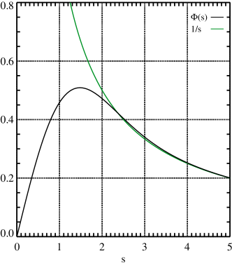
Figure 17: Graphical illustration of the functions $\Phi(s)$ (black; defined in Eq. (A22) and $1/s$ (green). The velocity perturbations $\textsl{v}_{y}$ are exactly proportional to the former function in the inner region and approximately proportional to the latter one in the outer region for $|y/a|\ll 1$. For $s\gtrsim 2.5$ both functions are very similar.

The solution of Eq. (A20) can be written as an integral over an auxiliary variable $u$ (Goedbloed et al., 2010):

$$\Phi=\frac{s}{2}\int^{1}_{0}(1-u^{2})^{-1/4}e^{-s^{2}u/2}\mathrm{d}u.$$ (A22)

The function $\Phi$ (black line in Fig. 17) is positive for $s>0$, and has a global maximum at $s_{\rm max}\approx 1.48$. Moreover, $\Phi(s)\approx 1.06/\sqrt{\pi}\,s$ for $s\ll 1$, and $\Phi(s)\approx 1/s$ for $s\gg 1$.

To obtain the final form of the velocity perturbations, $\textsl{v}_{y}$, in the inner layer (given by Eqs. A16 and A22), we need to determine the TM growth rate $\gamma$. It can be calculated by matching the inner and outer solutions of $\textsl{v}_{y}$ (the former given by Eq. (A9) at a certain point $y_{\mathrm{m}}$ in the region (marked in yellow in Fig. 8), where both solutions are valid and overlap, i.e. where they give the same predictions for both the velocity and the magnetic field perturbations. The value of $y_{\mathrm{m}}$ must be large enough, so that $\Phi(s)$ can be approximated as $\Phi(s)\approx s^{-1}$, i.e. $s\gg 1$, yet small enough that the outer ideal MHD solution behaves like $\textsl{v}_{y}\propto y^{-1}$ (for $y\rightarrow 0$). Moreover, the inner resistive solution was found for such small values of $y$ that $b_{0x}(y)$ can be approximated by Eq. (85). Hence, $y_{\mathrm{m}}\ll a$ must hold. Recalling that $s=1$ for $y=\epsilon_{\mathrm{R}}$, we can combine the above conditions into

$$\epsilon_{\mathrm{R}}\ll y_{\mathrm{m}}\ll a.$$ (A23)

The remaining part of the matching procedure is conceptually rather straightforward. Comparing Eqs. (A22) and (A9) at $y_{\mathrm{m}}$, we can determine the tearing mode growth rate $\gamma$. We omit the details of these calculations and only give here the final expression for the TM growth rate in resistive (-inviscid) MHD:

$$\gamma=\left(\frac{2}{2.12}\right)^{4/5}\eta^{3/5}\left(\frac{b_{0}k}{\sqrt{\rho_{0}}}\right)^{2/5}a^{-6/5}\left(\frac{1}{a\,k}-a\,k\right)^{4/5}.$$ (A24)

For $a\,k>1$, the growth rate is complex (because of the last factor), i.e. the system is TM unstable only for perturbations with wavevectors $a\,k<1$. On the other hand, for $a\,k\rightarrow 0$ the growth rate given by Eq. (A24) diverges, but in this regime the constant $\psi$ approximation becomes invalid and Eq. (A24) no longer holds.

We note that the width of the resistive layer is somewhat arbitrary. Some authors (cf. Goedbloed et al., 2010; Schnack, 2009) define the layer extend to $|y|=\epsilon_{\mathrm{R}}$, whereas we define its boundary to be located at

$$|y|=L_{\mathrm{R}}=1.48\epsilon_{\mathrm{R}},$$ (A25)

which corresponds to the maximum of $\Phi(s)$ (Fig. 17). This is a convenient definition, because $\Phi(s_{\rm max})$ corresponds to the peaks of $\textsl{v}_{y}$, which can be determined from simulations rather easily (compare Fig. 17 with the bottom panels of Fig. 10).

Eqs. (A9) and (A22) for the velocity perturbation $\textsl{v}_{y}$, and Eq. (A8) for the magnetic field perturbation $b_{1y}$ (supplemented by Eq. (A24) and the transformations (A15) and (A16) constitute a complete solution of the TM problem in resistive MHD. In the inner layer, the magnetic field perturbation $b_{1y}$ is approximately constant, i.e. $b_{1y}(y\leq y_{\mathrm{m}})\approx b_{1y}(y_{\mathrm{m}})$, and the perturbations $\textsl{v}_{x}$ and $b_{1x}$ can be determined from conditions (79) and (80), respectively.

As a next step, we will generalise the above results to resistive-viscous MHD, because Eq. (A24) does not take into account (numerical) viscosity which might be comparable to (or even larger than) numerical resistivity.

A.1.3 Viscous Case

The derivation of the TM solution in resistive-viscous MHD by FKR63 is very similar to that of the non-viscous case. Therefore, we will only sketch their procedure (for more details see FKR63). One integrates Eqs. (A3) and (A4) again separately in the outer and inner region. In the outer region, one can neglect dissipative terms and plasma inertia as in the inviscid case, i.e. the magnetic field perturbation $b_{1y}$ and the velocity perturbation $\textsl{v}_{y}$ are still given by Eqs. (A8) and (A9), respectively. In the inner region, FKR63 simplified the sixth-order ODE (A12) for $\textsl{v}_{y}$ using again the constant $\psi$ approximation to a fourth-order ODE, but now including viscous terms. They further simplified the ODE by neglecting terms with lower-order derivatives, which is an acceptable approximation for magnetic Prandtl numbers $P_{\mathrm{m}}\equiv\nu/\eta\gtrsim 1$. Next, FKR63 introduced the dimensionless variables

$$\tilde{s} =\frac{y}{\epsilon_{\mathrm{RV}}},$$ (A26)

$$\tilde{\Phi} \propto\textsl{v}_{1y},$$ (A27)

(where we used the tilde symbol to explicitly stress that functions A22 and A27 differ) with the length scale

$$\epsilon_{\mathrm{RV}}=(\eta\nu)^{1/6}\left(\frac{a\sqrt{\rho_{0}}}{b_{0}k}\right)^{1/3}.$$ (A28)

The latter expression shows that both resistivity and viscosity affect the size of the region, where dissipative effects are important. We call this region the resistive-viscous layer. The width of this layer $L_{{\mathrm{RV}}}$ is proportional to $\epsilon_{\mathrm{RV}}$, and hence differs from the width $L_{{\mathrm{R}}}$ of the resistive (inviscid) layer, which is proportional to $\epsilon_{\mathrm{R}}$ (Eq. A19).

In the resistive-viscous case, matching condition (A23) has to be replaced by

$$\epsilon_{\mathrm{RV}}\ll y_{\mathrm{m}}\ll a,$$ (A29)

and from matching of $\tilde{\Phi}(\tilde{s})$ with Eq. (A9), we obtain the TM growth rate in resistive-viscous MHD:

$$\gamma\approx\frac{2^{4/3}}{3}\eta^{5/6}\nu^{-1/6}\left(\frac{b_{0}k}{\sqrt{\rho_{0}}}\right)^{1/3}a^{-4/3}\left(\frac{1}{a\,k}-a\,k\right).$$ (A30)

The above expression differs from the result of FKR63 (see their Eq. (H.8)), because these authors derived their equation in the $a\,k\ll 1$ limit (in our units), whereas we did not neglect terms proportional to $a\,k$. For the background magnetic field $b_{0x}=b_{0}\tanh(y/a)$, we calculated the growth rate more accurately. Note that Eq. (A30) is only an approximation, because FKR63 only approximately solved ODE (A12). Therefore, the above equation could be off by a small constant numerical factor.

Our numerical results differ from the analytic growth-rates derived above. Restrictions of grid resolution and computing time prevented us from reaching the parameter regime where the derivation of the analytic growth rates holds. Therefore, in the following subsection, we present an “empirical” ansatz for the TM growth rate which gives much better predictions for our simulation results presented in Sec. 4.3.

A.2 Empirical Approach

In the analytically derived Eqs. (A24) and (A30), the TM growth rate is proportional to a product of different powers of resistivity, viscosity, Alfvén speed, $a,k$, and $(1/(a\,k)-a\,k)$. Based on this observation, we postulate an ansatz:

$$\gamma=N_{0}\eta^{n_{1}}\nu^{n_{2}}\left(\frac{b_{0}}{\sqrt{\rho_{0}}}\right)^{n_{3}}k^{n_{4}}a^{n_{5}}\left(\frac{1}{a\,k}-a\,k\right)^{n_{6}},$$ (A31)

where $N_{0}$ is a (real) constant and $n_{1},\dots,n_{6}$ are fractional constants, which shall be determined by numerical simulations. The dimension of the growth rate is $[s^{-1}]$, which we abbreviate as $\mathrm{dim}(\gamma)=[\textrm{s}^{-1}]$. It has to be “constructed” from the other physical quantities. Since $\mathrm{dim}(\eta)=\mathrm{dim}(\nu)=[\textrm{cm}^{2}\ \textrm{s}^{-1}]$, $\mathrm{dim}(c_{\mathrm{A}})=[\textrm{cm}\ \textrm{s}^{-1}]$, $\mathrm{dim}(k)=[\textrm{cm}^{-1}]$, and $\mathrm{dim}(a)=[\textrm{cm}]$, dimensional analysis provides the following conditions:

$$n_{1}+n_{2}+n_{3} =1,$$ (A32)

$$2(n_{1}+n_{2})+n_{3}-n_{4}+n_{5} =0.$$ (A33)

Similarly, the width $L_{\mathrm{RV}}$ of the resistive-viscous layer should be equal to

$$L_{{\mathrm{RV}}}=M_{0}\epsilon_{\mathrm{RV}}=M_{0}\eta^{m_{1}}\nu^{m_{2}}\left(\frac{b_{0}}{\sqrt{\rho_{0}}}\right)^{m_{3}}k^{m_{4}}a^{m_{5}}\left(\frac{1}{a\,k}-a\,k\right)^{m_{6}},$$ (A34)

where $M_{0}$ is a (real positive) constant and $m_{1},\dots,m_{6}$ are fractional numbers to be determined by simulations. From the dimensional analysis follows

$$m_{1}+m_{2}+m_{3} =0,$$ (A35)

$$2(m_{1}+m_{2})+m_{3}-m_{4}+m_{5} =1.$$ (A36)

Table 6: 2D simulations performed to test and calibrate ansatz (A31) and (A34). The columns give the series identifier, shear parameter $a$, initial magnetic field strength $b_{0}$, viscosity $\nu$, and resistivity $\eta$. In all simulations the background density is set to $\rho_{0}=1$, and an equidistant grid spacing of $\Delta x=\Delta y=(\pi/3)/1024$ is used. The box length is $2L=20\,\pi a/3$ and the TM wavevector $k=3/(10a)$. The estimators $n_{i}$, $N_{i}$, $m_{i}$, and $M_{i}$ are given by fits according to Eqs. (A37), (A38), (A42), and (A43), respectively. In #TMa the estimators $n_{1}$, $N_{1}^{\mathrm{a}}$, $m_{1}$, and $M_{1}^{\mathrm{a}}$ are determined, whereas in #TMar the estimators $n_{1}$ and $m_{1}$ are set to fractional values and $N_{1}^{\mathrm{ar}}$ and $N_{1}^{\mathrm{ar}}$ are determined. For series #TMb, #TMc, and #TMd we proceeded analogously.

series	$a$	$b_{0}$	$\nu$	$\eta$	$n_{i}$	$N_{i}$	$m_{i}$	$M_{i}$
#TMa	$0.1$	$1$	$10^{-4}$	$10^{-7}\dots 10^{-5}$	$0.7994\pm 0.0012$	$5.377\pm 0.015$	$0.160\pm 0.003$	$-2.08\pm 0.04$
#TMar	$0.1$	$1$	$10^{-4}$	$10^{-7}\dots 10^{-5}$	$4/5$	$5.385\pm 0.001$	$1/6$	$-1.992\pm 0.004$
#TMb	$0.1$	$1$	$10^{-5}$	$10^{-6}\dots 10^{-5}$	$0.801\pm 0.004$	$5.84\pm 0.05$	$0.159\pm 0.007$	$-2.393\pm 0.006$
#TMbr	$0.1$	$1$	$10^{-5}$	$10^{-6}\dots 10^{-5}$	$4/5$	$5.826\pm 0.003$	$1/6$	$-2.393\pm 0.006$
#TMc	$0.1$	$0.5\dots 10$	$10^{-4}$	$5\times 10^{-5}$	$0.391\pm 0.004$	$-4.377\pm 0.006$	$-0.364\pm 0.017$	$-4.021\pm 0.015$
#TMcr	$0.1$	$0.5\dots 10$	$10^{-4}$	$5\times 10^{-5}$	$2/5$	$-4.385\pm 0.006$	$-1/3$	$-4.03\pm 0.02$
#TMd	$0.05$	$0.5\dots 4$	$10^{-5}$	$10^{-6}$	$0.411\pm 0.008$	$-4.058\pm 0.005$	$-0.329\pm 0.017$	$-5.17\pm 0.01$
#TMdr	$0.05$	$0.5\dots 4$	$10^{-5}$	$10^{-6}$	$2/5$	$-4.055\pm 0.005$	$-1/3$	$-5.17\pm 0.01$

To determine $n_{1}$ and $m_{1}$, we performed the simulations series #TMa (the setup is described in Tab. 6 and the results are given in Fig. 11, where the solid lines are the theoretical predictions according to Eqs. A48 and A49) keeping all parameters constant but the resistivity. To the measured TM growth rates and widths of the resistive-viscous layer (as described in Sec. 4.3.2), we fit functions

$$\ln(\gamma) =n_{1}\ln(\eta)+N_{1},$$ (A37)

$$\ln(L_{{\mathrm{RV}}}) =m_{1}\ln(\eta)+M_{1},$$ (A38)

where according to ansatzes (A31) and (A34) $N_{1}$ and $M_{1}$ should be constant for the models of series #TMa, i.e.

$$N_{1} =\ln\left[N_{0}\nu^{n_{2}}\left(\frac{b_{0}}{\sqrt{\rho_{0}}}\right)^{n_{3}}k^{n_{4}}a^{n_{5}}\left(\frac{\delta}{k}-\frac{k}{\delta}\right)^{n_{6}}\right],$$ (A39)

$$M_{1} =\ln\left[M_{0}\nu^{m_{2}}\left(\frac{b_{0}}{\sqrt{\rho_{0}}}\right)^{m_{3}}k^{m_{4}}a^{m_{5}}\left(\frac{1}{a\,k}-\frac{a\,k}{1}\right)^{m_{6}}\right].$$ (A40)

From the obtained estimators (and their small errors; see Tab. 6) $N_{1}^{\mathrm{a}}$ and $M_{1}^{\mathrm{a}}$ (the upper index “a” denotes the simulation series, i.e. #TMa), we conclude that our ansatzes hold (at least for resistivity) and that $n_{1}=4/5$ and $m_{1}=1/6$.

In the simulation series #TMb (Fig. 11), we set the value of the viscosity to $\nu=10^{-5}$, keeping the other parameters as in #TMa, and also vary the value of the resistivity. The fits done according to Eqs. (A37) and (A38) (see Tab. 6) confirm that $n_{1}=4/5$ and $m_{1}=1/6$.

We determine the dependence of the TM growth rate and of the width of the resistive-viscous layer on viscosity in the following somewhat indirect way. To the results of simulations #TMa, we refit functions (A37) and (A38), but this time with $n_{1}\equiv 4/5$ and $m_{1}\equiv 1/6$, to obtain $N_{1}^{\mathrm{ar}}$ and $M_{1}^{\mathrm{ar}}$, respectively (Tab. 6; note that we denote this series as #TMar, where “r” stands for “refitted”). In an analogous way, we obtain $N_{1}^{\mathrm{br}}$ and $M_{1}^{\mathrm{br}}$. According to ansatz (A31), the difference between $N_{1}^{\mathrm{ar}}$ and $N_{1}^{\mathrm{br}}$ should be

$$N_{1}^{\mathrm{ar}}-N_{1}^{\mathrm{br}}=\ln(10^{-4n_{2}})-\ln(10^{-5n_{2}})=n_{2}\ln(10).$$ (A41)

From the obtained estimators (Tab. 6), we have $N_{1}^{\mathrm{ar}}-N_{1}^{\mathrm{br}}=-0.441\pm 0.004$, from which we can infer $n_{2}=-1/5$. Analogously, from $M_{1}^{\mathrm{ar}}-M_{1}^{\mathrm{br}}=0.40\pm 0.01$, we infer that $m_{2}=1/6$ (theoretically this value should be $M_{1}^{\mathrm{ar}}-M_{1}^{\mathrm{br}}=(1/6)\ln(10)\approx 0.384$).

In two further sets of simulations (#TMc and #TMd), we determined the dependence of the TM growth rate and of the width of the resistive-viscous layer on the strength of the background magnetic field. To the simulation results (Fig. 18), we fit functions

$$\ln(\gamma) =n_{3}\ln(b_{0})+N_{3},$$ (A42)

$$\ln(L_{{\mathrm{RV}}}) =m_{3}\ln(b_{0})+M_{3},$$ (A43)

where $N_{3}$ and $M_{3}$ should be constant for a given simulation series.

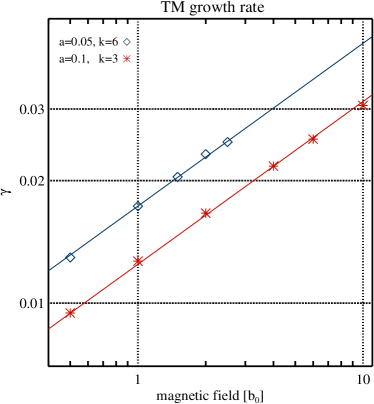
MM

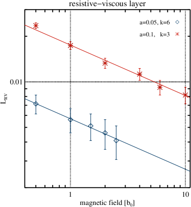
Figure 18: TM growth rate (left) and resistive-viscous layer width (right) as a function of background magnetic field strength. Simulations #TMd and #TMc are depicted with blue diamonds and red asterisks, respectively. Straight lines of the corresponding colours are linear fits to the logarithms of the simulation data.

From the obtained estimators (Tab. 6), we infer that $n_{3}=2/5$ and $m_{3}=-1/3$. Note that these results are consistent with our ansatzes, as from condition (A32), by putting $n_{1}=4/5$ and $n_{2}=-1/5$, we find $n_{3}=1-(n_{1}+n_{2})=2/5$, and analogously from condition (A35) we have $m_{3}=-m_{1}-m_{2}=-1/3$, as $m_{1}=m_{2}=1/6$.

With the results of simulation series #TMc and #TMd, one more aspect of Eqs. (A31) and (A34) can be tested. Even though we have not determined $n_{4},n_{5},n_{6}$ and $m_{4},m_{5},n_{6}$, we expect from dimensional analysis that $n_{4}-n_{5}=8/5$ and $m_{4}-m_{5}=-2/3$ (Eqs. A33 and A36, respectively). Therefore, doubling $a^{-1}$ and $k$ (from $a=0.1$, $k=3$ to $a=0.05$, $k=6$) should increase the instability growth rate by a factor of $2^{8/5}$ and decrease the width of the resistive-viscous layer by a factor of $2^{-2/3}$ (because for a constant $a$ to $k$ ratio, the term $(1/(a\,k)-a\,k)^{n_{6}}$ in Eq. A31 does not change). To the results of simulations #TMc and #TMd, we refitted functions (A42) and (A43), but this time with $n_{3}\equiv 2/5$ and $m_{3}\equiv-1/3$, obtaining (Tab. 6) $\Delta_{\mathrm{N3}}^{\mathrm{sim}}\equiv N_{3}^{\mathrm{cr}}-N_{3}^{\mathrm{dr}}=0.330\pm 0.011$ and $\Delta_{\mathrm{M3}}^{\mathrm{sim}}\equiv M_{3}^{\mathrm{cr}}-M_{3}^{\mathrm{dr}}=1.14\pm 0.03$. Taking into account the different values of resistivity and viscosity in these two series of simulations, we theoretically expect $\Delta_{\mathrm{N3}}^{\mathrm{th}}\equiv N_{3}^{\mathrm{cr}}-N_{3}^{\mathrm{dr}}=0.282$ and $\Delta_{\mathrm{M3}}^{\mathrm{th}}\equiv M_{3}^{\mathrm{cr}}-M_{3}^{\mathrm{dr}}=1.11$. Hence, the difference between theory and simulation is

$$\Delta_{\mathrm{N3}}^{\mathrm{th}}-\Delta_{\mathrm{N3}}^{\mathrm{sim}} =-0.048\pm 0.011,$$ (A44)

$$\Delta_{\mathrm{M3}}^{\mathrm{th}}-\Delta_{\mathrm{M3}}^{\mathrm{sim}} =-0.03\pm 0.03.$$ (A45)

Hence, the predictions for the resistive-viscous layer agree within the measurement error. Moreover, we tested that, as theoretically expected, in the parameter range explored by us (incompressible limit), the growth rate of the TM does neither depend on the background pressure $p_{0}$ nor on the bulk viscosity (see Rembiasz, 2013, for details).

So far, we have confirmed that our ansatzes for the TM growth rate (Eq. A31) and the width of the resistive-viscous layer (Eq. A34) hold and are given by

$$\gamma =N_{0}\eta^{4/5}\nu^{-1/5}\left(\frac{b_{0}}{\sqrt{\rho_{0}}}\right)^{2/5}k^{n_{4}}a^{n_{5}}\left(\frac{1}{a\,k}-\frac{a\,k}{1}\right)^{n_{6}},$$ (A46)

$$L_{{\mathrm{RV}}} =M_{0}(\eta\nu)^{1/6}\left(\frac{b_{0}}{\sqrt{\rho_{0}}}\right)^{-1/3}k^{m_{4}}a^{m_{5}}\left(\frac{1}{a\,k}-\frac{a\,k}{1}\right)^{m_{6}},$$ (A47)

where $N_{0}$ and $M_{0}$ are (real) constants, and $n_{4},n_{5},n_{6}$ and $m_{4},m_{5}$ are fractions. Moreover, from conditions (A33) and (A36) we have $n_{4}-n_{5}=8/5$ and $m_{4}-m_{5}=-2/3$, respectively. This allows us to calibrate these equations with the help of estimators $N_{1}^{\mathrm{ar}}$ and $M_{1}^{\mathrm{ar}}$ (Tab. 6) for $k=3$ and $a=0.1$ obtaining

$$\gamma(k=3,a=0.1) =34.56\eta^{4/5}\nu^{-1/5}\left(\frac{b_{0}}{\sqrt{\rho_{0}}}\right)^{2/5},$$ (A48)

$$L_{{\mathrm{RV}}}(k=3,a=0.1) =0.634(\eta\nu)^{1/6}\left(\frac{b_{0}}{\sqrt{\rho_{0}}}\right)^{-1/3}.$$ (A49)

References

- Aloy, Pons, & Ibáñez (1999) Aloy M. A., Pons J. A., Ibáñez J. M., 1999, CoPhC, 120, 115
- Abdikamalov et al. (2015) Abdikamalov E., et al., 2015, ApJ, 808, 70
- Akiyama et al. (2003) Akiyama S., Wheeler J. C., Meier D. L., Lichtenstadt I., 2003, ApJ, 584, 954
- Balbus & Hawley (1991) Balbus, S. A. & Hawley, J. F. 1991, ApJ, 376, 214
- Bodenheimer, Laughlin, Rozyczka, Plewa & Yorke (2006) Bodenheimer, P., Laughlin, G. P., Rozyczka, M., Plewa, T., & Yorke, H.W. 2006, Numerical Methods in Astrophysics: An Introduction (CRC Press)
- Buchmüller & Helzel (2014) Buchmüller P. & Helzel C., 2014, J Sci Comput, 61, 343
- Burrows, Hayes, & Fryxell (1995) Burrows A., Hayes J., Fryxell B. A., 1995, ApJ, 450, 830
- Campos (1999) Campos, L. M. B. C. 1999, Physics of Plasmas, 6, 57
- Cerdá-Durán, Font, & Dimmelmeier (2007) Cerdá-Durán P., Font J. A., Dimmelmeier H., 2007, A&A, 474, 169
- Chandrasekhar (1960) Chandrasekhar, S. 1960, Proceedings of the National Academy of Science, 46, 253
- Colella et al. (2011) Colella, P., Dorr, M. R., Hittinger, J. A. F., & Martin, D. F. 2011, Journal of Computational Physics, 230, 2952
- Couch & Ott (2015) Couch S. M., Ott C. D., 2015, ApJ, 799, 5
- Del Zanna et al. (2016) Del Zanna, L., Papini, E., Landi, S., Bugli, M., & Bucciantini, N. 2016, arXiv:1605.06331
- Evans & Hawley (1988) Evans, C. R. & Hawley, J. F. 1988, ApJ, 332, 659
- Foglizzo, Scheck, & Janka (2006) Foglizzo T., Scheck L., Janka H.-T., 2006, ApJ, 652, 1436
- Fureby & Grinstein (1999) Fureby C., Grinstein F. F., 1999, AIAAJ, 37, 544
- Furth et al. (1963) Furth, H. P., Killeen, J., & Rosenbluth, M. N. 1963, Physics of Fluids, 6, 459
- Goodman & Xu (1994) Goodman, J. & Xu, G. 1994, ApJ, 432, 213
- Guilet et al. (2015) Guilet, J., Müller, E. & Janka, H. T. 2015, ApJ, 447, 3992
- Guilet & Müller (2015) Guilet J., Müller E., 2015, MNRAS, 450, 2153
- Goedbloed & Poedts (2004) Goedbloed, J. P. H. & Poedts, S. 2004, Principles of Magnetohydrodynamics (Cambridge University Press)
- Goedbloed et al. (2010) Goedbloed, J. P., Keppens, R., & Poedts, S. 2010, Advanced Magnetohydrodynamics (Cambridge University Press)
- Harten (1983) Harten, A. 1983, J. Comput. Phys., 49, 357
- Herant (1995) Herant M., 1995, PhR, 256, 117
- Hou & Le Floch (1994) Hou, T. Y. & Le Floch, P. G. 1994, Math. of Computation, 62, 497
- Janka & Müller (1996) Janka H.-T., Müller E., 1996, A&A, 306, 167
- Landau & Lifshitz (1982) Landau, L. D., Lifshitz, E. M. 1982, Course of theoretical physics, Vol. 6: Fluid mechanics (Pergamon Press)
- Landau & Lifshitz (1970) Landau, L. D., Lifshitz, E. M. 1970 , Course of theoretical physics, Vol. 7: Theory of elasticity (Pergamon Press)
- Landi et al. (2008) Landi, S., Londrillo, P., Velli, M., & Bettarini, L. 2008, Physics of Plasmas, 15, 012302
- Landi et al. (2015) Landi, S., Del Zanna, L., Papini, E., Pucci, F., & Velli, M. 2015, ApJ, 806, 131
- Laney (1998) Laney, C. 1998, Computational Gasdynamics (Cambridge University Press)
- Latter et al. (2009) Latter, H. N., Lesaffre, P., & Balbus, S. A. 2009, MNRAS, 394, 715
- LeVeque (1992) LeVeque, R. J. 1992, Numerical Methods for Conservation Laws, 2nd edn., Lectures in mathematics - ETH Zürich (Birkhäuser)
- LeVeque (2002) LeVeque, R. J. 2002, Finite Volume Methods for Hyperbolic Problems (Cambridge University Press)
- Levy et al. (2002) Levy, D., Puppo, G., & Russo, G. 2002, SIAM J. Sci. Comput., 24, 480
- McCorquodale & Colella (2011) McCorquodale, P. & Colella, P. 2011, Communications in Applied Mathematics and Computational Science, Vol. 6, No. 1, 1
- Mimica et al. (2009) Mimica, P., Giannios, D., & Aloy. M- A. 2009, A&A, 494, 879
- Miyoshi & Kusano (2005) Miyoshi, T. & Kusano, K. 2005, Journal of Computational Physics, 208, 315
- Mösta et al. (2015) Mösta, P. and Ott, C. D. and Radice, et al. 2015, Nature, 528, 376
- Murphy, Dolence, & Burrows (2013) Murphy J. W., Dolence J. C., Burrows A., 2013, ApJ, 771, 52
- Obergaulinger (2008) Obergaulinger, M. 2008, PhD thesis, Technische Universität München. https://mediatum.ub.tum.de/doc/632729/632729.pdf
- Obergaulinger et al. (2006) Obergaulinger M., Aloy M. A., Dimmelmeier H., Müller E., 2006, A&A, 457, 209
- Obergaulinger et al. (2009) Obergaulinger, M., Cerdá-Durán, P., Müller, E., & Aloy, M. A. 2009, A&A, 498, 241
- Obergaulinger, Janka, & Aloy (2014) Obergaulinger M., Janka H.-T., Aloy M. A., 2014, MNRAS, 445, 3169
- Pessah & Goodman (2009) Pessah, M. E., & Goodman, J. 2009, ApJ, 698, L72
- Pessah (2010) Pessah, M. E. 2010, ApJ, 716, 1012
- Peterson & Hammett (2013) Peterson, J. L., Hammett, G. W. 2013, SIAM J. Sci. Comput., 35(3), B576-B605
- Priest & Forbes (2007) Priest, E., & Forbes, T. 2007, Magnetic Reconnection, by Eric Priest , Terry Forbes, Cambridge, UK: Cambridge University Press, 2007,
- Pucci & Velli (2014) Pucci, F., & Velli, M. 2014, ApJ, 780, L19
- Radice, Couch, & Ott (2015) Radice D., Couch S. M., Ott C. D., 2015, ComAC, 2, 7
- Rembiasz (2013) Rembiasz, T. 2013, PhD thesis, Technische Universität München. https://mediatum.ub.tum.de/doc/1183388
- Rembiasz et al. (2016a) Rembiasz T., Obergaulinger M., Cerdá-Durán P., Müller E., Aloy M. A., 2016, MNRAS, 456, 3782
- Rembiasz et al. (2016b) Rembiasz T., Guilet J., Obergaulinger M., Cerdá-Durán P., Aloy M. A., Müller E., 2016, MNRAS.
- Sawai & Yamada (2016) Sawai H., Yamada S., 2016, ApJ, 817, 153
- Sawai, Yamada, & Suzuki (2013) Sawai H., Yamada S., Suzuki H., 2013, ApJ, 770, L19
- Schnack (2009) Schnack, D. D. 2009, Lectures in Magnetohydrodynamics by Dalton D. Schnack, Springer, ISBN: 978-3-642-00687-6,
- Shore (2007) Shore, S. N. 2007, Astrophysical Hydrodynamics: An Introduction (Wiley-VCH)
- Shu (1997) Shu, C.-W. 1997, ICASE Report No.97-65
- Shu & Osher (1988) Shu C.-W., Osher S., 1988, J. Comput. Phys., 77, 439
- Suresh & Huynh (1997) Suresh, A. & Huynh, H. 1997, J. Comput. Phys., 136, 83
- Toro (1997) Toro, E. 1997, Riemann Solvers and Numerical Methods for Fluid Dynamics (Berlin: Springer)
- Toro & Titarev (2006) Toro, E. F. & Titarev, V. A. 2006, J. Comput. Phys., 216, 403
- Velikhov (1959) Velikhov, E. 1959, Sov. Phys. JETP, 36, 995
- Zhang et al. (2011) Zhang, R., Zhang M., Shu C.-W., 2011, Commun. Comput. Phys., 9, 807-827
- Zhou et al. (2014) Zhou Y., Grinstein F. F., Wachtor A. J., Haines B. M., 2014, PhRvE, 89, 013303