A Generalized Stochastic Variational Bayesian Hyperparameter Learning Framework for Sparse Spectrum Gaussian Process Regression

Abstract

While much research effort has been dedicated to scaling up sparse Gaussian process (GP) models based on inducing variables for big data, little attention is afforded to the other less explored class of low-rank GP approximations that exploit the sparse spectral representation of a GP kernel. This paper presents such an effort to advance the state of the art of sparse spectrum GP models to achieve competitive predictive performance for massive datasets. Our generalized framework of stochastic variational Bayesian sparse spectrum GP ($s$VBSSGP) models addresses their shortcomings by adopting a Bayesian treatment of the spectral frequencies to avoid overfitting, modeling these frequencies jointly in its variational distribution to enable their interaction a posteriori, and exploiting local data for boosting the predictive performance. However, such structural improvements result in a variational lower bound that is intractable to be optimized. To resolve this, we exploit a variational parameterization trick to make it amenable to stochastic optimization. Interestingly, the resulting stochastic gradient has a linearly decomposable structure that can be exploited to refine our stochastic optimization method to incur constant time per iteration while preserving its property of being an unbiased estimator of the exact gradient of the variational lower bound. Empirical evaluation on real-world datasets shows that $s$VBSSGP outperforms state-of-the-art stochastic implementations of sparse GP models.

1 Introduction

The machine learning community has recently witnessed the Gaussian process (GP) models gaining considerable traction in the research on kernel methods due to its expressive power and capability of performing probabilistic non-linear regression. However, a full-rank GP regression model incurs cubic time in the size of the data to compute its predictive distribution, hence limiting its use to small datasets. To lift this computational curse, a vast literature of sparse GP regression models (?; ?) have exploited a structural assumption of conditional independence based on the notion of inducing variables for achieving linear time in the data size. To scale up these sparse GP regression models further for performing real-time predictions necessary in many time-critical applications and decision support systems (e.g., environmental sensing (?; ?; ?; ?; ?; ?; ?; ?; ?), traffic monitoring (?; ?; ?; ?; ?; ?; ?; ?; ?; ?)), (a) distributed (?; ?; ?) and (b) stochastic (?; ?) implementations of such models have been developed to, respectively, (a) reduce their time to train with all the data by a factor close to the number of machines and (b) train with a small, randomly sampled subset of data in constant time per iteration of stochastic gradient ascent update and achieve asymptotic convergence to their predictive distributions.

On the other hand, there is a less well-explored, alternative class of low-rank GP approximations that exploit sparsity in the spectral representation of a GP kernel (?; ?) for gaining time efficiency and have empirically demonstrated competitive predictive performance for datasets of up to tens of thousands in size but, surprisingly, not received as much attention and research effort. In contrast to the above literature, such sparse spectrum GP regression models do not need to introduce an additional set of inducing inputs which is computationally challenging to be jointly optimized, especially with a large number of them that is necessary for accurate predictions. Unfortunately, the sparse spectrum GP (SSGP) model of ? (?) does not scale well to massive datasets due to its linear time in the data size and also finds a point estimate of the spectral frequencies of its kernel that risks overfitting. The recent variational SSGP (VSSGP) model of ? (?) has attempted to address both shortcomings of SSGP with a stochastic implementation and a Bayesian treatment of the spectral frequencies, respectively. However, VSSGP has imposed the following highly restrictive structural assumptions to facilitate analytical derivations but potentially compromise its predictive performance: (a) The spectral frequencies are assumed to be fully independent a posteriori in its variational distribution, and (b) every test output assumes a deterministic relationship with the spectral frequencies in its test conditional and is thus conditionally independent of the training data, including the local data “close” to it (in the correlation sense). As such, open questions remain whether VSSGP can still perform competitively well with these highly restrictive structural assumptions for massive, million-sized datasets and, more importantly, whether these assumptions can be relaxed to improve the predictive performance while preserving scalability to big data.

To tackle these questions, this paper presents a novel generalized framework of stochastic variational Bayesian sparse spectrum GP ($s$VBSSGP) regression models which (a) enables the spectral frequencies to interact a posteriori by modeling them jointly in its variational distribution, and (b) spans a spectrum of test conditionals that can trade off between the contributions of the degenerate test conditional of VSSGP vs. the local SSGP model trained with local data (Section 2). However, such proposed structural improvements over VSSGP and SSGP to boost the predictive performance result in a variational lower bound that is intractable to be optimized. To overcome this computational difficulty, we exploit a variational parameterization trick to make the variational lower bound amenable to stochastic optimization, which still incurs linear time in the data size per iteration of stochastic gradient ascent update (Section 3). Interestingly, we can exploit the linearly decomposable structure of this stochastic gradient to refine our stochastic optimization method to incur only constant time per iteration while preserving its property of being an unbiased estimator of the exact gradient of the variational lower bound (Section 4). We empirically evaluate the predictive performance and time efficiency of $s$VBSSGP on three real-world datasets, one of which is millions in size (Section 5).

2 A Generalized Bayesian Sparse Spectrum Gaussian Process Regression Framework

Let $\mathcal{X}$ be a $d$-dimensional input space such that each input vector $\mathbf{x}\in\mathcal{X}$ is associated with a latent output $f_{\mathbf{x}}$ and a noisy output $y_{\mathbf{x}}\triangleq f_{\mathbf{x}}+\epsilon$ generated by perturbing $f_{\mathbf{x}}$ with a random noise $\epsilon\sim\mathcal{N}(0,\sigma_{n}^{2})$ where $\sigma_{n}^{2}$ is the noise variance. Let $\{f_{\mathbf{x}}\}_{\mathbf{x}\in\mathcal{X}}$ denote a Gaussian process (GP), that is, every finite subset of $\{f_{\mathbf{x}}\}_{\mathbf{x}\in\mathcal{X}}$ follows a multivariate Gaussian distribution. Then, the GP is fully specified by its prior mean $\mathbb{E}[f_{\mathbf{x}}]$ (i.e., assumed to be $0$ for notational simplicity) and covariance $k(\mathbf{x},\mathbf{x}^{\prime})\triangleq\text{cov}[f_{\mathbf{x}},f_{\mathbf{x}^{\prime}}]$ for all $\mathbf{x},\mathbf{x}^{\prime}\in\mathcal{X}$, the latter of which can be defined by the commonly-used squared exponential kernel $k(\mathbf{x},\mathbf{x}^{\prime})\triangleq\sigma^{2}_{s}\mathrm{exp}(-0.5(\mathbf{x}-\mathbf{x^{\prime}})^{\top}\bm{\Delta}^{-1}(\mathbf{x}-\mathbf{x^{\prime}}))$ where $\bm{\Delta}\triangleq\mathrm{diag}[\ell_{1}^{2},\ell_{2}^{2},\ldots,\ell_{d}^{2}]$ and $\sigma^{2}_{s}$ are its squared length-scale and signal variance hyperparameters, respectively. Such a kernel can be expressed as the Fourier transform of a density function $p(\mathbf{r})$ over the domain of frequency vector $\mathbf{r}$ whose coefficients form a set of trigonometric basis functions (?):

$$k(\mathbf{x},\mathbf{x}^{\prime})=\mathbb{E}_{\mathbf{r}\sim p(\mathbf{r})}[\ \sigma^{2}_{s}\mathrm{cos}(2\pi\mathbf{r}^{\top}(\mathbf{x}-\mathbf{x}^{\prime}))\ ]$$ (1)

where $p(\mathbf{r})\triangleq\mathcal{N}\left(\mathbf{0},(4\pi^{2}\bm{\Delta})^{-1}\right)$. In the same spirit as that of ? (?), we approximate the kernel in (1) by its unbiased estimator constructed from $m$ i.i.d. sampled spectral frequencies $\mathbf{r}_{i}$ for $i=1,\ldots,m$:

$$\begin{array}[]{l}\displaystyle k(\mathbf{x},\mathbf{x}^{\prime})\simeq\frac{\sigma^{2}_{s}}{m}\sum^{m}_{i=1}\mathrm{cos}(2\pi\mathbf{r}^{\top}_{i}(\mathbf{x}-\mathbf{x}^{\prime}))=\bm{\phi}^{\top}_{{\bm{\theta}}}(\mathbf{x})\bm{\Lambda}\bm{\phi}_{{\bm{\theta}}}(\mathbf{x^{\prime}})\vspace{-0mm}\end{array}\vspace{-1mm}$$ (2)

where $\bm{\phi}_{\bm{\theta}}(\mathbf{x})\triangleq[\phi^{1}_{\bm{\theta}}(\mathbf{x}),\phi^{2}_{\bm{\theta}}(\mathbf{x}),\ldots,\phi^{2m}_{\bm{\theta}}(\mathbf{x})]^{\top}$ denotes a vector of basis functions $\phi^{2i-1}_{\bm{\theta}}(\mathbf{x})\triangleq\cos(2\pi\mathbf{r}_{i}^{\top}\mathbf{x})$ and $\phi^{2i}_{\bm{\theta}}(\mathbf{x})\triangleq\sin(2\pi\mathbf{r}_{i}^{\top}\mathbf{x})$ for $i=1,\ldots,m$, $\bm{\Lambda}\triangleq(\sigma^{2}_{s}/m)\mathbf{I}$, and ${\bm{\theta}}\triangleq\mathrm{vec}(\mathbf{r}_{1},\mathbf{r}_{2},\ldots,\mathbf{r}_{m})$. Learning the length-scales in $\bm{\Delta}$ of the original kernel is thus cast as optimizing ${\bm{\theta}}$ in this alternative representation (2) of the kernel. Then, the induced covariance matrix $\mathbf{K}(\mathbf{X},\mathbf{X})$ for any finite subset $\mathbf{X}\triangleq\{\mathbf{x}_{i}\}_{i=1}^{n}$ of training inputs can be written as $\mathbf{K}(\mathbf{X},\mathbf{X})\triangleq\mathbf{\Phi}_{\bm{\theta}}^{\top}(\mathbf{X})\mathbf{\Lambda}\mathbf{\Phi}_{\bm{\theta}}(\mathbf{X})$ where $\mathbf{\Phi}_{\bm{\theta}}(\mathbf{X})\triangleq[\bm{\phi}_{\bm{\theta}}(\mathbf{x}_{1})\ldots\bm{\phi}_{\bm{\theta}}(\mathbf{x}_{n})]$.

To learn the optimal parameters of the distribution over ${\bm{\theta}}$ (i.e., not known in advance) given by $\mathcal{N}(\mathbf{0},(4\pi^{2}\bm{\Delta}_{\bm{\theta}})^{-1})$ (i.e., derived from $p(\mathbf{r})$ below (1)) where $\bm{\Delta}_{\bm{\theta}}\triangleq\mathbf{I}\otimes\bm{\Delta}$, we adopt the standard Bayesian treatment for ${\bm{\theta}}$ by first imposing a prior distribution ${\bm{\theta}}\sim\mathcal{N}(\mathbf{0},{\bm{\Theta}})$ for some covariance ${\bm{\Theta}}$ designed a priori to reflect our knowledge about ${\bm{\theta}}$ and then using training data to infer its posterior which is expected to closely approximate the optimal distribution. This signifies a key difference between our generalized framework and the sparse spectrum GP (SSGP) model of ? (?), the latter of which finds a point estimate of ${\bm{\theta}}$ via maximum likelihood estimation that risks overfitting.

As shall be elucidated later in this paper, the finite trigonometric representation of the kernel (2) can be used to efficiently and scalably compute the predictive distribution of our framework by exploiting some mild structural assumptions. Specifically, we assume that for any finite subset $\mathbf{X}\subset\mathcal{X}$, a vector $\mathbf{s}$ of nuisance variables exists for which the joint distribution of $\mathbf{f}\triangleq[f_{\mathbf{x}}]^{\top}_{\mathbf{x}\in\mathbf{X}}$ and $\mathbf{s}$ conditioned on ${\bm{\theta}}$ is

$$\left[\begin{array}[]{l}\mathbf{s}\\ \mathbf{f}\end{array}\right]\hskip 0.7113pt\sim\hskip 0.7113pt\mathcal{N}\left(\left[\begin{array}[]{l}\mathbf{0}\\ \mathbf{0}\end{array}\right],\left[\begin{array}[]{cc}\bm{\Lambda}&\bm{\Lambda}\bm{\Phi}_{\bm{\theta}}(\mathbf{X})\\ \bm{\Phi}^{\top}_{\bm{\theta}}(\mathbf{X})\bm{\Lambda}&\bm{\Phi}^{\top}_{\bm{\theta}}(\mathbf{X})\bm{\Lambda}\bm{\Phi}_{\bm{\theta}}(\mathbf{X})\end{array}\right]\right).$$ (3)

Intuitively, $\mathbf{s}$ can be interpreted as the latent outputs of some imaginary inputs $\mathbf{U}\triangleq\{\mathbf{u}_{j}\}_{j=1}^{2m}$ such that $\phi^{i}_{\bm{\theta}}(\mathbf{u}_{j})\triangleq\mathbb{I}(i=j)$. Using (2), it follows immediately that $\mathbf{K}(\mathbf{U},\mathbf{U})=\bm{\Lambda}$, $\mathbf{K}(\mathbf{U},\mathbf{X})=\bm{\Lambda}\bm{\Phi}_{\bm{\theta}}(\mathbf{X})$, and $\mathbf{K}(\mathbf{X},\mathbf{U})=\bm{\Phi}^{\top}_{\bm{\theta}}(\mathbf{X})\bm{\Lambda}$ which reproduce the covariance matrix in (3). Secondly, we assume that given $\bm{\alpha}\triangleq\mathrm{vec}({\bm{\theta}},\mathbf{s})$, any latent test output depends on only a small subset of local training data of fixed size: Supposing the input space is partitioned into $p$ disjoint sub-spaces (i.e., $\mathcal{X}=\bigcup_{i=1}^{p}\mathcal{X}_{i}$) which directly induce a partition on the training inputs $\mathbf{X}=\bigcup_{i=1}^{p}\mathbf{X}_{i}$ such that $\mathbf{X}_{i}\subset\mathcal{X}_{i}$, $p(f_{\mathbf{x}_{\ast}}|\mathbf{y},\bm{\alpha})=p(f_{\mathbf{x}_{\ast}}|\mathbf{y}_{k},\bm{\alpha})$ for any test input $\mathbf{x}_{\ast}\in\mathcal{X}_{k}$ and $k=1,\ldots,p$ where $\mathbf{y}\triangleq[y_{\mathbf{x}}]^{\top}_{\mathbf{x}\in\mathbf{X}}$ and $\mathbf{y}_{k}\triangleq[y_{\mathbf{x}}]^{\top}_{\mathbf{x}\in\mathbf{X}_{k}}$. Then, the predictive distribution can be computed using

$$p(f_{\mathbf{x}_{*}}|\mathbf{y})=\mathbb{E}_{\bm{\alpha}\sim p(\bm{\alpha}|\mathbf{y})}[\ p(f_{\mathbf{x}_{*}}|\mathbf{y}_{k},\bm{\alpha})\ ]$$ (4)

which reveals that it can be evaluated by deriving posterior distribution $p(\bm{\alpha}|\mathbf{y})$ described later in Section 3, and the test conditional $p(f_{\mathbf{x}_{*}}|\mathbf{y}_{k},\bm{\alpha})$ consistent with the above structural assumption of $\mathbf{s}$: Marginalizing out nuisance variables $\mathbf{s}$ from such a test conditional should yield $p(f_{\mathbf{x_{\ast}}}|\mathbf{y}_{k},{\bm{\theta}})$, i.e., $p(f_{\mathbf{x_{\ast}}}|\mathbf{y}_{k},{\bm{\theta}})=\int_{\mathbf{s}}\ p(f_{\mathbf{x}_{*}}|\mathbf{y}_{k},\bm{\alpha})\ p(\mathbf{s}|\mathbf{y}_{k},{\bm{\theta}})\ \mathrm{d}\mathbf{s}$ where both $p(f_{\mathbf{x_{\ast}}}|\mathbf{y}_{k},{\bm{\theta}})$ and $p(\mathbf{s}|\mathbf{y}_{k},{\bm{\theta}})$ can be derived from (3), as shown in Appendix A.

Our first result below derives a spectrum of consistent test conditionals in our generalized framework that trade off between the use of global information $\bm{\alpha}$ vs. local data $(\mathbf{X}_{k},\mathbf{y}_{k})$, albeit to varying degrees controlled by $\gamma$:

Proposition 1

For all $\mathbf{x_{\ast}}\in\mathcal{X}_{k}$ and $|\gamma|\leq 1$, define the test conditional $p(f_{\mathbf{x_{\ast}}}|\mathbf{y}_{k},\bm{\alpha})\triangleq\mathcal{N}(\mu_{\mathbf{x}_{\ast}}(\bm{\alpha}),\sigma^{2}_{\mathbf{x}_{\ast}}(\bm{\alpha}))$ where

$$\begin{array}[]{rcl}\mu_{\mathbf{x}_{\ast}}(\bm{\alpha})&\triangleq&\displaystyle\gamma\bm{\phi}^{\top}_{\bm{\theta}}(\mathbf{x_{\ast}})\mathbf{s}+(1-\gamma)\bm{\phi}^{\top}_{\bm{\theta}}(\mathbf{x_{\ast}})\bm{\Gamma}^{-1}_{k}\bm{\Phi}_{\bm{\theta}}(\mathbf{X}_{k})\mathbf{y}_{k}\ ,\vspace{0.5mm}\\ \sigma^{2}_{\mathbf{x}_{\ast}}(\bm{\alpha})&\triangleq&\displaystyle(1-\gamma^{2})\sigma^{2}_{n}\bm{\phi}^{\top}_{\bm{\theta}}(\mathbf{x_{\ast}})\bm{\Gamma}^{-1}_{k}\bm{\phi}_{\bm{\theta}}(\mathbf{x_{\ast}})\ ,\end{array}$$

and $\bm{\Gamma}_{k}\triangleq\bm{\Phi}_{\bm{\theta}}(\mathbf{X}_{k})\bm{\Phi}_{\bm{\theta}}^{\top}(\mathbf{X}_{k})+\sigma_{n}^{2}\bm{\Lambda}^{-1}$. Then, $p(f_{\mathbf{x_{\ast}}}|\mathbf{y}_{k},\bm{\alpha})$ is consistent with the structural assumption of $\mathbf{s}$ in (3).

Its proof is in Appendix A.

Remark 1 The special case of $\gamma=1$ recovers the degenerate test conditional $p(f_{\mathbf{x}_{\ast}}|\bm{\alpha})=\mathcal{N}(\bm{\phi}_{\bm{\theta}}^{\top}(\mathbf{x}_{\ast})\mathbf{s},0)$ induced by the variational SSGP (VSSGP) model of ? (?) (see equation $4$ and Section $3$ therein) which reveals that it imposes a highly restrictive deterministic relationship between $f_{\mathbf{x}_{\ast}}$ and $\bm{\alpha}$ and also fails to exploit the local data $(\mathbf{X}_{k},\mathbf{y}_{k})$ (i.e., due to conditional independence between $f_{\mathbf{x}_{\ast}}$ and $\mathbf{y}_{k}$ given $\bm{\alpha}$) that can potentially improve the predictive performance. Unfortunately, VSSGP cannot be trivially extended to span the entire spectrum since it relies on the induced deterministic relationship between $f_{\mathbf{x}_{\ast}}$ and $\bm{\alpha}$ to analytically derive its predictive distribution, which does not hold for $\gamma\neq 1$. On the other hand, when $\gamma=0$, the test conditional in Proposition 1 becomes independent of the nuisance variables $\mathbf{s}$ and reduces to the predictive distribution $p(f_{\mathbf{x_{\ast}}}|\mathbf{y}_{k},\bm{\theta})$ of the SSGP model of ? (?) (see equation $7$ therein) given its point estimate of the spectral frequencies ${\bm{\theta}}$ but restricted to the local data $(\mathbf{X}_{k},\mathbf{y}_{k})$ corresponding to input subspace $\mathcal{X}_{k}$. Hence, $\gamma$ can also be perceived as a controlling parameter that trades off between the contributions of the degenerate test conditional of VSSGP vs. the local SSGP model to constructing a test conditional in our generalized framework. To investigate this trade-off, our experiments in Section 5 show that given the learned ${\bm{\theta}}$, the predictive performance is maximized at $\gamma=0$ when the test conditional $p(f_{\mathbf{x_{\ast}}}|\mathbf{y}_{k},\bm{\alpha})$ depends on local data $(\mathbf{X}_{k},\mathbf{y}_{k})$ but not $\mathbf{s}$, which justifies viewing $\mathbf{s}$ as a “nuisance” to prediction despite its crucial role in scalable learning of ${\bm{\theta}}$ via stochastic optimization (Section 4).

In the sections to follow, we will propose a novel stochastic optimization method for deriving a variationally optimal approximation to the posterior distribution $p(\bm{\alpha}|\mathbf{y})$ that is used to marginalize out the global information $\bm{\alpha}$ from any test conditional $p(f_{\mathbf{x_{\ast}}}|\mathbf{y}_{k},\bm{\alpha})$ in Proposition 1 to yield an asymptotic approximation to the predictive distribution $p(f_{\mathbf{x_{\ast}}}|\mathbf{y})$ (4) regardless of the value of $\gamma\in[-1,1]$.

3 Variational Inference for Bayesian Sparse Spectrum Gaussian Process Regression

This section presents a variational approximation $q(\bm{\alpha})$ of the posterior distribution $p(\bm{\alpha}|\mathbf{y})$ achieved by using variational inference which involves choosing a parameterization for $q(\bm{\alpha})$ (Section 3.1) and optimizing its defining parameters (Section 3.2) to minimize its Kullback-Leibler (KL) distance ${D}_{\mathrm{KL}}(q)\triangleq\mathrm{KL}(q(\bm{\alpha})\|p(\bm{\alpha}|\mathbf{y}))$ to $p(\bm{\alpha}|\mathbf{y})$. The optimized $q(\bm{\alpha})$ can then be used as a tractably cheap surrogate of $p(\bm{\alpha}|\mathbf{y})$ for marginalizing out $\bm{\alpha}$ from test conditional $p(f_{\mathbf{x_{\ast}}}|\mathbf{y}_{k},\bm{\alpha})$ in Proposition 1 to derive an approximation to predictive distribution $p(f_{\mathbf{x_{\ast}}}|\mathbf{y})$ (4) efficiently (Section 4).

3.1 Variational Parameterization

Specifically, we parameterize $\bm{\alpha}=\mathrm{vec}({\bm{\theta}},\mathbf{s})\triangleq\mathbf{Mz+b}$ where the variational parameters $\bm{\eta}\triangleq\mathrm{vec}(\mathbf{M},\mathbf{b})$ are independent of $({\bm{\theta}},\mathbf{s})$, and $\mathbf{z}$ is distributed by an analytically tractable user-specified distribution $\psi(\mathbf{z})\simeq p(\mathbf{z}|\mathbf{y})$ that is straightforward to draw samples from (i.e., $\mathbf{z}\sim\psi(\mathbf{z})$). We assume that $\psi(\mathbf{z})$ is analytically differentiable with respect to $\mathbf{z}$ and the affine matrix $\mathbf{M}$ is invertible such that $\mathbf{z}=\mathbf{M}^{-1}(\bm{\alpha}-\mathbf{b})$ exists. Then, $q({\bm{\theta}},\mathbf{s})$ can be expressed in terms of $\mathbf{M}$, $\mathbf{b}$, and $\psi(\mathbf{z})$:

Lemma 1

The variational distribution $q({\bm{\theta}},\mathbf{s})$ can be indirectly parameterized via $\psi(\mathbf{z})$ by $q({\bm{\theta}},\mathbf{s})=q(\bm{\alpha})=\psi(\mathbf{M}^{-1}(\bm{\alpha}-\mathbf{b}))/|\mathbf{M}|=\psi(\mathbf{z})/|\mathbf{M}|$ where $|\mathbf{M}|$ denotes the absolute value of $\mathrm{det}(\mathbf{M})$.

Lemma 1 follows directly from the change of variables theorem. Using the above parameterization of $\bm{\alpha}$, we can also express the prior $p({\bm{\theta}},\mathbf{s})$ in terms of variational parameters $\mathbf{M}$ and $\mathbf{b}$. To see this, recall that $p({\bm{\theta}})=\mathcal{N}(\mathbf{0},{\bm{\Theta}})$ and $p(\mathbf{s})=\mathcal{N}(\mathbf{0},\bm{\Lambda})$ (see Section 2 and (3)). This implies $p(\bm{\alpha})=p(\mathrm{vec}({\bm{\theta}},\mathbf{s}))=p({\bm{\theta}})\ p(\mathbf{s})=\mathcal{N}(\bm{\alpha}|\mathbf{0},\mathrm{blkdiag}[{\bm{\Theta}},\bm{\Lambda}])$. Plugging in the expression of $\bm{\alpha}$ yields $p(\bm{\alpha})=\mathcal{N}(\mathbf{M}\mathbf{z}+\mathbf{b}|\mathbf{0},\mathrm{blkdiag}[{\bm{\Theta}},\bm{\Lambda}])$. At this time, the need to parameterize $q(\bm{\alpha})$ in Lemma 1 may not be obvious to a reader because it is motivated by a technical necessity to guarantee the asymptotic convergence of our stochastic optimization method (Remark $4$) rather than a conceptual intuition.

Remark 2 Our generalized framework enables both the spectral frequencies ${\bm{\theta}}$ and the nuisance variables $\mathbf{s}$ to interact a posteriori by modeling them jointly in the variational distribution $q({\bm{\theta}},\mathbf{s})$, as detailed in Lemma 1, and still preserves scalability (Section 4). In contrast, the VSSGP model of ? (?) assumes $\mathbf{r}_{1},\ldots,\mathbf{r}_{m},\text{and}\ \mathbf{s}$ to be statistically independent a posteriori in its variational distribution (see section $4$ therein). Relaxing this assumption will cause VSSGP to lose its scalability as its induced variational lower bound will inevitably become intractable.

Remark 3 Though the model of ? (?) has adopted a similar parameterization but only for the original GP hyperparameters, it incurs cubic time in the data size per iteration of gradient ascent update, as shown in its supplementary materials and experiments. A factorized marginal likelihood has to be further assumed for this parameterization to achieve scalability. Our framework does not require such a strong assumption and still scales well to million-sized datasets (Section 5). This is, perhaps surprisingly, achieved through introducing the nuisance variables $\mathbf{s}$ (Section 2), which interestingly embeds a linearly decomposable structure within the log-likelihood of data $\log p(\mathbf{y}|\bm{\alpha})$ instead of $\log p(\mathbf{y}|{\bm{\theta}})$. As shown later in Theorem 1, such a structure is the key ingredient for developing our stochastic optimization method (Section 4).

3.2 Variational Optimization

To optimize $q(\bm{\alpha})$ (i.e., by minimizing ${D}_{\mathrm{KL}}(q)$), we first show that the log-marginal likelihood $\log p(\mathbf{y})$ can be decomposed into a sum of a lower-bound functional ${L}(q)$ and ${D}_{\mathrm{KL}}(q)$: $\log p(\mathbf{y})={L}(q)+{D}_{\mathrm{KL}}(q)$ where ${L}(q)\triangleq\mathbb{E}_{\bm{\alpha}\sim q(\bm{\alpha})}[\log p(\mathbf{y}|\bm{\alpha})-\log({q(\bm{\alpha})}/{p(\bm{\alpha})})]$, as detailed in Appendix B. So, minimizing ${D}_{\mathrm{KL}}(q)$ is equivalent to maximizing ${L}(q)$ with respect to the variational parameter $\bm{\eta}=\mathrm{vec}(\mathbf{M},\mathbf{b})$ of $q(\bm{\alpha})$ (Lemma 1) since $\log p(\mathbf{y})$ is a constant (i.e., independent of $\bm{\eta}$). In practice, this is usually achieved by setting the derivative $\partial{L}/\partial\bm{\eta}=0$ and solving for $\bm{\eta}$, which is unfortunately intractable since its exact analytic expression is not known.

To sidestep this intractability issue, we instead adopt a stochastic optimization method that is capable of maximizing ${L}(q)$ via iterative stochastic gradient ascent updates. However, this also requires the stochastic gradient $\partial\widehat{{L}}/\partial\bm{\eta}$ (6) to be an analytically tractable and unbiased estimator of the exact gradient $\partial{L}/\partial\bm{\eta}$. To derive this, we first exploit Lemma 1 to re-express ${L}(q)$ as an expectation with respect to $\mathbf{z}\sim\psi(\mathbf{z})$: ${L}(q)=\mathbb{E}_{\mathbf{z}\sim\psi(\mathbf{z})}[\log p(\mathbf{y}|\bm{\alpha})-\log({q(\bm{\alpha})}/{p(\bm{\alpha})})]$ where $\bm{\alpha}=\mathbf{M}\mathbf{z}+\mathbf{b}$, as shown in Appendix C. Then, taking the derivatives with respect to $\bm{\eta}$ on both sides of the above equation yields

$$\partial{L}/\partial\bm{\eta}=\mathbb{E}_{\mathbf{z}\sim\psi(\mathbf{z})}[\ \partial(\log p(\mathbf{y}|\bm{\alpha})-\log(q(\bm{\alpha})/p(\bm{\alpha})))/\partial\bm{\eta}\ ]$$ (5)

which reveals a simple, analytically tractable (proven in Appendix D using Lemma 1) choice for our stochastic gradient

$$\partial\widehat{{L}}/\partial\bm{\eta}\triangleq\partial(\log p(\mathbf{y}|\bm{\alpha})-\log(q(\bm{\alpha})/p(\bm{\alpha})))/\partial\bm{\eta}\ .$$ (6)

Thus, $\mathbb{E}_{\mathbf{z}\sim\psi(\mathbf{z})}[\partial\widehat{{L}}/\partial\bm{\eta}]=\partial{L}/\partial\bm{\eta}$ guarantees that $\partial\widehat{{L}}/\partial\bm{\eta}$ is indeed an unbiased estimator of $\partial{L}/\partial\bm{\eta}$.

Remark 4 (5) reveals that parameterizing $q(\bm{\alpha})$ indirectly through $\psi(\mathbf{z})$ in Lemma 1 is essential to enabling stochastic optimization in our generalized framework: Since $\psi(\mathbf{z})$ does not depend on the variational parameters $\bm{\eta}=\mathrm{vec}(\mathbf{M},\mathbf{b})$, the derivative operator in (5) can be moved inside the expectation, which trivially reveals an unbiased stochastic estimate (6) of the exact gradient via sampling $\mathbf{z}$. Otherwise, suppose that we attempt to derive a stochastic gradient for ${L}(q)$ using the original expression ${L}(q)=\mathbb{E}_{\bm{\alpha}\sim q(\bm{\alpha})}[\log p(\mathbf{y}|\bm{\alpha})-\log({q(\bm{\alpha})}/{p(\bm{\alpha})})]$ instead of (5) in the same manner with a direct parameterization of $q(\bm{\alpha})$ not exploiting $\psi(\mathbf{z})$. Then, after differentiating both sides of the above expression with respect to $\bm{\eta}$, the derivative operator on the RHS cannot be moved inside the expectation over $\bm{\alpha}\sim q(\bm{\alpha})$ since it depends on $\bm{\eta}$, which suggests that deriving an unbiased estimator for $\partial{L}/\partial\bm{\eta}$ has become non-trivial without using the parameterization of $q(\bm{\alpha})$ in Lemma 1.

To understand why ${\partial\widehat{{L}}}/{\partial\bm{\eta}}$ (6) is analytically tractable, it suffices to show that both its derivatives $\partial\log p(\mathbf{y}|\bm{\alpha})/\partial\bm{\eta}$ and $\partial\log(q(\bm{\alpha})/p(\bm{\alpha}))/\partial\bm{\eta}$ in (6) are analytically tractable, the latter of which is detailed in Appendix D. For the former, since the trigonometric basis functions $\{\phi_{\bm{\theta}}^{i}(\mathbf{x})\}_{i=1}^{2m}$ (Section 2) are differentiable, it can be shown that $\partial\log p(\mathbf{y}|\bm{\alpha})/\partial\bm{\eta}$ is analytically tractable by exploiting the following result giving a closed-form expression of $\log p(\mathbf{y}|\bm{\alpha})$ in terms of ${\bm{\theta}}$ and $\mathbf{s}$:

Lemma 2

$\log p(\mathbf{y}|\bm{\alpha})=-0.5\sigma_{n}^{-2}\mathbf{v}^{\top}\mathbf{v}-0.5n\log(2\pi\sigma_{n}^{2})$ where $\mathbf{v}\triangleq\mathbf{y}-\bm{\Phi}^{\top}_{\bm{\theta}}(\mathbf{X})\mathbf{s}$.

Its proof is in Appendix E. The above choice of ${\partial\widehat{{L}}}/{\partial\bm{\eta}}$ (6) and Lemma 2 show that it is not only an unbiased estimator of the exact gradient but is also analytically tractable, which satisfies all the required conditions to guarantee the asymptotic convergence of our proposed stochastic optimization method. However, a critical issue remains that makes it scale poorly in practice: It can be derived from Lemma 2 that naively evaluating its derivative $\partial\log p(\mathbf{y}|\bm{\alpha})/\partial\bm{\eta}$ in (6) in a straightforward manner incurs linear time in data size $n$ per iteration of stochastic gradient ascent update, which is expensive for massive datasets.

4 Stochastic Optimization

To overcome the issue of scalability in evaluating the stochastic gradient ${\partial\widehat{{L}}}/{\partial\bm{\eta}}$ (6) (Section 3.2), we will show in Theorem 1 below that $\partial\log p(\mathbf{y}|\bm{\alpha})/\partial\bm{\eta}$ is decomposable into a linear sum of analytically tractable terms, each of which depends on only a small subset of local data. Interestingly, since only the derivative $\partial\log p(\mathbf{y}|\bm{\alpha})/\partial\bm{\eta}$ in (6) involves the training data $(\mathbf{X},\mathbf{y})$, Theorem 1 implies a similar decomposition of $\partial\widehat{{L}}/\partial\bm{\eta}$. As a result, we can derive a new stochastic estimate of the exact gradient $\partial{L}/\partial\bm{\eta}$ that can be computed efficiently and scalably using only one or a few randomly sampled subset(s) of local data of fixed size and still preserves the property of being its unbiased estimator (Section 4.1). Computing this new stochastic gradient incurs only constant time in the data size $n$ per iteration of stochastic gradient ascent update, which, together with Proposition 1 in Section 2, constitute the foundation of our generalized framework of stochastic variational Bayesian SSGP regression models for big data (Section 4.2).

4.1 Stochastic Gradient Revisited

To derive a computationally scalable and unbiased stochastic gradient, we rely on our main result below showing the decomposability of $\partial\log p(\mathbf{y}|\bm{\alpha})/\partial\bm{\eta}$ in (6) into a linear sum of analytically tractable terms, each of which depends on only a small subset of local training data of fixed size:

Theorem 1

Let $\mathbf{v}_{i}\triangleq\mathbf{y}_{i}-\bm{\Phi}^{\top}_{\bm{\theta}}(\mathbf{X}_{i})\mathbf{s}$ for $i=1,\ldots,p$. Then, $\partial\log p(\mathbf{y}|\bm{\alpha})/\partial\bm{\eta}=\sum_{i=1}^{p}{F}_{i}(\bm{\eta},\bm{\alpha})$ where ${F}_{i}(\bm{\eta},\bm{\alpha})\triangleq-0.5\sigma_{n}^{-2}\nabla_{\bm{\eta}}(\mathbf{v}^{\top}_{i}\mathbf{v}_{i})$ is analytically tractable.

Its proof in Appendix F utilizes Lemma 2. Using Theorem 1 , the following linearly decomposable structure of ${\partial\widehat{{L}}}/{\partial\bm{\eta}}$ (6) results:

$$\partial\widehat{{L}}/\partial\bm{\eta}=\mathbb{E}_{i\sim\mathcal{U}(1,p)}[\ p{F}_{i}(\bm{\eta},\bm{\alpha})-{\partial}\log(q(\bm{\alpha})/p(\bm{\alpha}))/\partial\bm{\eta}\ ]\vspace{-1mm}$$ (7)

where $i$ is treated as a discrete random variable uniformly distributed over the set of partition indices $\{1,2,\ldots,p\}$. This interestingly reveals an unbiased estimator for the stochastic gradient $\partial\widehat{{L}}/\partial\bm{\eta}$ which can be constructed stochastically by sampling $i$:

$${\partial\widetilde{{L}}}/{\partial\bm{\eta}}\triangleq p{F}_{i}(\bm{\eta},\bm{\alpha})-{\partial}\log({q(\bm{\alpha})}/{p(\bm{\alpha})})/{\partial\bm{\eta}}\vspace{-1mm}$$

such that substituting it into (7) yields $\mathbb{E}_{i\sim\mathcal{U}(1,p)}[\partial\widetilde{{L}}/\partial\bm{\eta}]=\partial\widehat{{L}}/\partial\bm{\eta}$. Then, taking the expectation over $\mathbf{z}\sim\psi(\mathbf{z})$ on both sides of this equality gives $\mathbb{E}_{\mathbf{z}\sim\psi(\mathbf{z})}[\mathbb{E}_{i\sim\mathcal{U}(1,p)}[\partial\widetilde{{L}}/\partial\bm{\eta}]]=\mathbb{E}_{\mathbf{z}\sim\psi(\mathbf{z})}[\partial\widehat{{L}}/\partial\bm{\eta}]=\partial{L}/\partial\bm{\eta}$, which proves that $\partial\widetilde{{L}}/\partial\bm{\eta}$ is also an unbiased estimator of $\partial{L}/\partial\bm{\eta}$ that can be constructed by sampling both $i\sim\mathcal{U}(1,p)$ and $\mathbf{z}\sim\psi(\mathbf{z})$ (Section 3.1) independently. Replacing $\partial\widehat{{L}}/\partial\bm{\eta}$ with $\partial\widetilde{{L}}/\partial\bm{\eta}$ produces a highly efficient stochastic gradient ascent update that incurs constant time in the data size $n$ per iteration since $\partial\widetilde{{L}}/\partial\bm{\eta}$ can be computed using only a single randomly sampled subset of local data $(\mathbf{X}_{i},\mathbf{y}_{i})$ of fixed size.

Instead of utilizing just a single pair $(i,\mathbf{z})$ of samples, the above stochastic gradient ${\partial\widetilde{{L}}}/{\partial\bm{\eta}}$ can be generalized to simultaneously process multiple pairs of independent samples and their corresponding sampled subsets of local data in one stochastic gradient ascent update (detailed in Appendix G), thereby improving the rate of convergence while preserving its property of an unbiased estimator of the exact gradient ${\partial{{L}}}/{\partial\bm{\eta}}$. Asymptotic convergence of the estimate of $\bm{\eta}$ (and hence the estimate of $q(\bm{\alpha})$) is guaranteed if the step sizes are scheduled appropriately.

4.2 Approximate Predictive Inference

In iteration $t$ of stochastic gradient ascent update, an estimate $q_{t}(\bm{\alpha})$ of the variationally optimal approximation $q(\bm{\alpha})$ can be induced from the current estimate $\bm{\eta}_{t}=\mathrm{vec}(\mathbf{M}_{t},\mathbf{b}_{t})$ of its variational parameters $\bm{\eta}$ using the parameterization in Lemma 1. As a result, using the law of iterated expectations, the predictive mean can be approximated by $\widehat{\mu}_{\mathbf{x}_{\ast}}=\mathbb{E}_{\bm{\alpha}\sim q_{t}(\bm{\alpha})}[\mathbb{E}[f_{\mathbf{x}_{\ast}}|\mathbf{y}_{k},\bm{\alpha}]]=\mathbb{E}_{\bm{\alpha}\sim q_{t}(\bm{\alpha})}[\mu_{\mathbf{x}_{\ast}}(\bm{\alpha})]=\int_{\bm{\alpha}}q_{t}(\bm{\alpha})\mu_{\mathbf{x}_{\ast}}(\bm{\alpha})\mathrm{d}\bm{\alpha}$ where $\bm{\alpha}=\mathrm{vec}({\bm{\theta}},\mathbf{s})$ and $\mu_{\mathbf{x}_{\ast}}(\bm{\alpha})$ is previously defined in Proposition 1. However, since the integration over $\bm{\alpha}$ is not always analytically tractable, we approximate it by drawing i.i.d. samples $\bm{\alpha}_{1},\ldots,\bm{\alpha}_{r}$ from $q_{t}(\bm{\alpha})$ to estimate $\widehat{\mu}_{\mathbf{x}_{\ast}}\simeq r^{-1}\sum_{i=1}^{r}\mu_{\mathbf{x}_{\ast}}(\bm{\alpha}_{i})$. Similarly, using the variance decomposition formula and definition of variance, the predictive variance can be approximated by $\widehat{\sigma}^{2}_{\mathbf{x}_{\ast}}=\mathbb{E}_{\bm{\alpha}\sim q_{t}(\bm{\alpha})}[\sigma^{2}_{\mathbf{x}_{\ast}}(\bm{\alpha})]+\mathbb{V}_{\bm{\alpha}\sim q_{t}(\bm{\alpha})}[\mu_{\mathbf{x}_{\ast}}(\bm{\alpha})]=\mathbb{E}_{\bm{\alpha}\sim q_{t}(\bm{\alpha})}[\sigma^{2}_{\mathbf{x}_{\ast}}(\bm{\alpha})+\mu^{2}_{\mathbf{x}_{\ast}}(\bm{\alpha})]-\widehat{\mu}^{2}_{\mathbf{x}_{\ast}}\simeq r^{-1}\sum_{i=1}^{r}(\sigma^{2}_{\mathbf{x}_{\ast}}(\bm{\alpha}_{i})+\mu^{2}_{\mathbf{x}_{\ast}}(\bm{\alpha}_{i}))-\widehat{\mu}^{2}_{\mathbf{x}_{\ast}}$ where $\sigma^{2}_{\mathbf{x}_{\ast}}(\bm{\alpha})$ is previously defined in Proposition 1 and the $\mathbb{V}_{\bm{\alpha}\sim q_{t}(\bm{\alpha})}[\mu_{\mathbf{x}_{\ast}}(\bm{\alpha})]$ term arises due to the uncertainty of $\bm{\alpha}$. The samples $\bm{\alpha}_{1},\ldots,\bm{\alpha}_{r}$ are in turn obtained by sampling $\mathbf{z}_{1},\ldots,\mathbf{z}_{r}$ from $\psi(\mathbf{z})$ and applying the parametric transformation in Lemma 1 with respect to the current estimates $\mathbf{M}_{t}$ and $\mathbf{b}_{t}$, that is, $\mathrm{vec}({\bm{\theta}}_{i},\mathbf{s}_{i})=\bm{\alpha}_{i}=\mathbf{M}_{t}\mathbf{z}_{i}+\mathbf{b}_{t}$ for $i=1,\ldots,r$. Computing the predictive mean $\widehat{\mu}_{\mathbf{x}_{\ast}}$ and variance $\widehat{\sigma}^{2}_{\mathbf{x}_{\ast}}$ thus incurs constant time in the data size $n$, hence achieving efficient approximate predictive inference.

5 Empirical Studies

This section empirically evaluates the predictive performance and time efficiency of our $s$VBSSGP model on three real-world datasets: (a) The AIMPEAK dataset (?) consists of $41800$ traffic speed observations (km/h) along $775$ urban road segments during the morning peak hours on April $20$, $2011$. Each observation features a $5$-dimensional input vector of a road segment’s length, number of lanes, speed limit, direction, and its recording time (i.e., discretized into $54$ five-minute time slots), and a corresponding output measuring the traffic speed (km/h); (b) the benchmark AIRLINE dataset (?; ?) contains $2000000$ information records of US commercial flights in $2008$. Each record features a $8$-dimensional input vector of the aircraft’s age (year), travel distance (km), the flight’s total airtime, departure time, arrival time (min), and the date given by day of week, day of month, and month, and a corresponding output of the flight’s delay time (min); and (c) the BLOG feedback dataset (?) contains $60000$ instances of blog posts. Each blog post features a fairly large $60$-dimensional input vector associated with its first $60$ attributes described at https://archive.ics.uci.edu/ml/datasets/BlogFeedback, and a corresponding output measuring the number of comments in the next $24$ hours. The BLOG dataset is used to evaluate the robustness of $s$VBSSGP to overfitting which usually occurs in training with datasets of high input dimensions. All datasets are modeled using GPs with prior covariance defined in Section 2 and split into $95\%$ training data and $5\%$ test data. All experimental results are averaged over $5$ random splits. For the AIMPEAK, AIRLINE, and BLOG datasets, we use, respectively, $2m=40,40,\text{and}\ 10$ trigonometric basis functions to approximate the GP kernel (2) and sample $\mathbf{z}$ from $\mathcal{N}(\mathbf{0},\mathbf{I})$ (Section 3.1). All experiments are run on a Linux system with Intel$\circledR$ Xeon$\circledR$ E$5$-$2670$ at $2.6$GHz with $96$ GB memory.

The performance of $s$VBSSGP is compared against the state-of-the-art VSSGP (?) and stochastic implementations of sparse GP models based on inducing variables such as DTC$+$ and PIC$+$ (?; ?) (i.e., run with their GitHub codes) using the following metrics: (a) Root mean square error (RMSE) $\{|\overline{\mathbf{X}}|^{-1}\sum_{\mathbf{x}_{*}\in\overline{\mathbf{X}}}(y_{\mathbf{x}_{*}}-\widehat{\mu}_{\mathbf{x}_{*}})^{2}\}^{1/2}$ over the set $\overline{\mathbf{X}}$ of test inputs, (b) mean negative log probability (MNLP) $0.5|\overline{\mathbf{X}}|^{-1}\sum_{{\mathbf{x}_{*}}\in\overline{\mathbf{X}}}\{(y_{\mathbf{x}_{*}}-\widehat{\mu}_{\mathbf{x}_{*}})^{2}/\widehat{\sigma}^{2}_{\mathbf{x}_{*}}+\mathrm{log}(2\pi\widehat{\sigma}^{2}_{\mathbf{x}_{*}})\}$, and (c) training time.

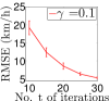
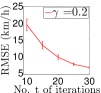
Figure 1: Graphs of RMSEs (with standard deviations) achieved by $s$VBSSGP vs. number $t$ of iterations with varying values of $\gamma$ for the AIMPEAK dataset.

AIMPEAK Dataset. This dataset is evenly partitioned into $p=200$ disjoint subsets using $k$-means ($k=p$). Fig. 1 shows results of RMSEs of $s$VBSSGP for $\gamma=0,0.1,0.2,0.3$ that rapidly decrease by $4$- to $5$-fold over $30$ iterations. It can also be observed that increasing $\gamma$ from $0$ results in higher converged RMSEs. To further investigate this, Fig. 2a reveals that $s$VBSSGP indeed achieves the lowest converged RMSE at $\gamma=0$ among all tested values of $\gamma$. This confirms our hypothesis stated earlier in Remark $1$ that given the learned spectral frequencies $\bm{\theta}$, the information carried by $\mathbf{s}$ becomes a “nuisance” to prediction despite its interaction with $\bm{\theta}$ in $q(\bm{\theta},\mathbf{s})=q(\bm{\alpha})$ during stochastic optimization. That is, when the influence of $\mathbf{s}$ on the test output is completely removed from the test conditional by setting $\gamma=0$ in Proposition 1, the predictions are no longer interfered by the nuisance information of $s$, hence explaining the lowest RMSE achieved by $s$VBSSGP at $\gamma=0$.

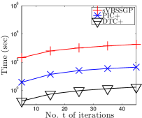
(a)	(b)	(c)	(d)

Figure 2: (a) Graph of RMSEs achieved by $s$VBSSGP vs. $\gamma$ for the AIMPEAK dataset; graphs of RMSEs achieved by $s$VBSSGP, PIC$+$, DTC$+$, and VSSGP vs. number $t$ of iterations for the (b) AIMPEAK and (c) AIRLINE datasets; and (d) graph of total training time incurred by $s$VBSSGP, PIC$+$, and DTC$+$ vs. number $t$ of iterations for the AIRLINE dataset.

Fig. 2b and Table 1 show that $s$VBSSGP ($\gamma=0$ and $r=20$) significantly outperforms VSSGP, DTC$+$, and PIC$+$ ($250$ inducing variables) in terms of RMSE after $30$ iterations. To explain this, DTC$+$ and PIC$+$ find point estimates of the kernel hyperparameters, which may have resulted in their poorer performance. Though VSSGP also adopts a Bayesian treatment of the spectral frequencies, it uses a degenerate test conditional corresponding to the case of $\gamma=1$ in Proposition 1. As a result, VSSGP imposes a highly restrictive deterministic relationship between the test output and spectral frequencies and also fails to exploit the local data for prediction (see Remark $1$). The results of the MNLP metric are similar and reported in Appendix H.

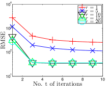
(a)	(b)

Figure 3: Graphs of RMSEs achieved by $s$VBSSGP vs. number $t$ of iterations with varying number $r$ of samples drawn from $q_{t}(\bm{\alpha})$ to compute predictive mean $\widehat{\mu}_{\mathbf{x}_{*}}$ (Section 4.2) for the (a) AIMPEAK and (b) BLOG datasets.

AIRLINE Dataset. This dataset is partitioned into $p=2000$ disjoint subsets using $k$-means. Fig. 2c and Table 1 show that $s$VBSSGP ($\gamma=0$ and $r=5$) significantly outperforms VSSGP, DTC$+$, and PIC$+$ ($512$ inducing variables) in terms of RMSE after $45$ iterations, as explained previously. Fig. 2d shows that the total training time of $s$VBSSGP increases linearly with the number $t$ of iterations, which highlights a principled trade-off between its predictive performance and time efficiency. The training time of $s$VBSSGP, though longer than DTC$+$ and PIC$+$, is only $43$ sec. per iteration; the training time of VSSGP is not included since its GitHub code runs on GPU instead of CPU. The results of MNLP metric are similar to that for the AIMPEAK dataset.

Dataset	$s$VBSSGP	DTC$+$	PIC$+$	SSGP	VSSGP
AIMPEAK	4.73	$12.46$	$6.15$	$11.30$	$9.46$
AIRLINE	22.18	$39.60$	$33.40$	n/a	$39.49$

Table 1: RMSEs achieved by $s$VBSSGP, DTC$+$, PIC$+$, SSGP (?), and VSSGP after final convergence for AIMPEAK and AIRLINE datasets.

BLOG Dataset. This dataset is evenly partitioned into $p=200$ disjoint subsets using $k$-means. Fig. 3 shows that with more samples drawn from $q_{t}(\bm{\alpha})$ to compute predictive mean $\widehat{\mu}_{\mathbf{x}_{*}}$ (Section 4.2), $s$VBSSGP tends to converge faster and to a lower RMSE, which suggests a greater robustness to overfitting by exploiting a higher degree of Bayesian model averaging. More interestingly, the effect of overfitting appears to be more pronounced for the BLOG dataset with a much larger input dimension of $60$: When $r=1$, $s$VBSSGP effectively reduces to a local SSGP model utilizing the sampled spectral frequencies as its point estimate (see Proposition 1, Remark $1$, and Section 4.2) and converges to the poorest performance that stops improving after $10$ iterations. It can also be observed that the performance gap between $s$VBSSGP’s with different number $r$ of samples is much wider at early iterations, thus highlighting the practicality of our Bayesian treatment in the case of limited data.

6 Conclusion

This paper describes a novel generalized framework of $s$VBSSGP regression models that addresses the shortcomings of existing sparse spectrum GP models like SSGP (?) and VSSGP (?) by adopting a Bayesian treatment of the spectral frequencies to avoid overfitting, modeling the spectral frequencies jointly in its variational distribution to enable their interaction a posteriori, and exploiting local data for improving the predictive performance while still being able to preserve its scalability to big data through stochastic optimization. As a result, empirical evaluation on real-world datasets (i.e., including the million-sized benchmark AIRLINE dataset) shows that our proposed $s$VBSSGP regression model can significantly outperform the existing sparse spectrum GP models like SSGP and VSSGP as well as the stochastic implementations of the sparse GP models based on inducing variables like DTC$+$ and PIC$+$ (?; ?).

Acknowledgments. This research is supported by the National Research Foundation, Prime Minister’s Office, Singapore under its International Research Centre in Singapore Funding Initiative and Campus for Research Excellence and Technological Enterprise (CREATE) programme.

Appendix A Proof of Proposition 1

Since $\{f_{\mathbf{x}}\}_{\mathbf{x}\in\mathcal{X}}$ denotes a zero-mean Gaussian process with kernel $k(\mathbf{x},\mathbf{x}^{\prime})$ and the noisy output $y_{\mathbf{x}}=f_{\mathbf{x}}+\epsilon$ is generated by perturbing $f_{\mathbf{x}}$ with a random noise $\epsilon\sim\mathcal{N}(0,\sigma_{n}^{2})$ (Section 2), $p(f_{\mathbf{x}_{\ast}}|\mathbf{y}_{k},{\bm{\theta}})=\mathcal{N}(\mathbb{E}[f_{\mathbf{x}_{\ast}}|\mathbf{y}_{k},{\bm{\theta}}],\mathbb{V}[f_{\mathbf{x}_{\ast}}|\mathbf{y}_{k},{\bm{\theta}}])$ for $\mathbf{x}_{\ast}\in\mathcal{X}_{k}$ where

$$\begin{array}[]{rcl}\mathbb{E}[f_{\mathbf{x}_{\ast}}|\mathbf{y}_{k},{\bm{\theta}}]&\triangleq&\displaystyle\mathbf{K}(\mathbf{x}_{\ast},\mathbf{X}_{k})\bm{\Xi}_{k}\mathbf{y}_{k}\ ,\vspace{0.5mm}\\ \mathbb{V}[f_{\mathbf{x}_{\ast}}|\mathbf{y}_{k},{\bm{\theta}}]&\triangleq&\displaystyle k(\mathbf{x_{\ast}},\mathbf{x_{\ast}})-\mathbf{K}(\mathbf{x_{\ast}},\mathbf{X}_{k})\bm{\Xi}_{k}\mathbf{K}(\mathbf{X}_{k},\mathbf{x}_{\ast})\ ,\end{array}$$ (8)

and $\bm{\Xi}_{k}\triangleq(\mathbf{K}(\mathbf{X}_{k},\mathbf{X}_{k})+\sigma_{n}^{2}\mathbf{I})^{-1}$, which is essentially the standard GP predictive distribution of $f_{\mathbf{x}_{\ast}}$ given the noisy outputs $\mathbf{y}_{k}$ for the training inputs $\mathbf{X}_{k}$ and the hyperparameters ${\bm{\theta}}$. Using (2),

$$\begin{array}[]{l}\bm{\Xi}_{k}\\ \displaystyle=(\bm{\Phi}_{\bm{\theta}}^{\top}(\mathbf{X}_{k})\bm{\Lambda}\bm{\Phi}_{\bm{\theta}}(\mathbf{X}_{k})+\sigma_{n}^{2}\mathbf{I})^{-1}\vspace{0.5mm}\\ \displaystyle=\sigma_{n}^{-2}\mathbf{I}-\sigma_{n}^{-4}\bm{\Phi}_{\bm{\theta}}^{\top}(\mathbf{X}_{k})(\sigma_{n}^{-2}\bm{\Phi}_{\bm{\theta}}(\mathbf{X}_{k})\bm{\Phi}_{\bm{\theta}}^{\top}(\mathbf{X}_{k})+\bm{\Lambda}^{-1})^{-1}\bm{\Phi}_{\bm{\theta}}(\mathbf{X}_{k})\\ \displaystyle=\sigma_{n}^{-2}(\mathbf{I}-\bm{\Phi}_{\bm{\theta}}^{\top}(\mathbf{X}_{k})\bm{\Gamma}^{-1}_{k}\bm{\Phi}_{\bm{\theta}}(\mathbf{X}_{k}))\end{array}$$

where the second and third equalities are due to the matrix inversion lemma and the definition of $\bm{\Gamma}_{k}$, respectively. Using (2), (8) can also be rewritten as

$$\begin{array}[]{rcl}\mathbb{E}\left[f_{\mathbf{x}_{\ast}}|\mathbf{y}_{k},{\bm{\theta}}\right]&=&\displaystyle\gamma\mathbf{H}\bm{\mu}+(1-\gamma)\mathbf{H}\bm{\mu}\\ \mathbb{V}\left[f_{\mathbf{x}_{\ast}}|\mathbf{y}_{k},{\bm{\theta}}\right]&=&\displaystyle(1-\gamma^{2})\mathbf{H}\bm{\Sigma}\mathbf{H}^{\top}+\gamma^{2}\mathbf{H}\bm{\Sigma}\mathbf{H}^{\top}\end{array}$$

for all $|\gamma|\leq 1$ where $\mathbf{H}\triangleq\bm{\phi}_{\bm{\theta}}^{\top}(\mathbf{x}_{\ast})$,

$$\begin{array}[]{rcl}\bm{\mu}&\triangleq&\displaystyle\bm{\Lambda}\bm{\Phi}_{\bm{\theta}}(\mathbf{X}_{k})\bm{\Xi}_{k}\mathbf{y}_{k}\\ &=&\displaystyle\sigma_{n}^{-2}\bm{\Lambda}(\mathbf{I}-\bm{\Phi}_{\bm{\theta}}(\mathbf{X}_{k})\bm{\Phi}_{\bm{\theta}}^{\top}(\mathbf{X}_{k})\bm{\Gamma}^{-1}_{k})\bm{\Phi}_{\bm{\theta}}(\mathbf{X}_{k})\mathbf{y}_{k}\\ &=&\displaystyle\sigma_{n}^{-2}\bm{\Lambda}(\mathbf{I}-(\bm{\Gamma}_{k}-\sigma^{2}_{n}\bm{\Lambda}^{-1})\bm{\Gamma}^{-1}_{k})\bm{\Phi}_{\bm{\theta}}(\mathbf{X}_{k})\mathbf{y}_{k}\\ &=&\displaystyle\bm{\Gamma}^{-1}_{k}\bm{\Phi}_{\bm{\theta}}(\mathbf{X}_{k})\mathbf{y}_{k}\end{array}$$

where the third equality is due to the definition of $\bm{\Gamma}_{k}$, and

$$\begin{array}[]{rcl}\mathbf{\Sigma}&\triangleq&\displaystyle\bm{\Lambda}-\bm{\Lambda}\bm{\Phi}_{\bm{\theta}}(\mathbf{X}_{k})\bm{\Xi}_{k}\bm{\Phi}_{\bm{\theta}}^{\top}(\mathbf{X}_{k})\bm{\Lambda}\\ &=&\displaystyle\bm{\Lambda}-\bm{\Gamma}^{-1}_{k}\bm{\Phi}_{\bm{\theta}}(\mathbf{X}_{k})\bm{\Phi}_{\bm{\theta}}^{\top}(\mathbf{X}_{k})\bm{\Lambda}\\ &=&\displaystyle\bm{\Lambda}-\bm{\Gamma}^{-1}_{k}(\bm{\Gamma}_{k}-\sigma^{2}_{n}\bm{\Lambda}^{-1})\bm{\Lambda}\\ &=&\displaystyle\sigma^{2}_{n}\bm{\Gamma}^{-1}_{k}\ .\end{array}$$

Using the Gaussian identity of affine transformation for marginalization,

$$p\left(f_{\mathbf{x}_{\ast}}|\mathbf{y}_{k},{\bm{\theta}}\right)=\int_{\mathbf{s}}\mathcal{N}\left(f_{\mathbf{x}_{\ast}}|\mu_{\mathbf{x}_{\ast}}(\bm{\alpha}),\sigma^{2}_{\mathbf{x}_{\ast}}(\bm{\alpha})\right)\mathcal{N}(\mathbf{s}|\bm{\mu},\bm{\Sigma})\ \mathrm{d}\mathbf{s}$$ (9)

where $\mu_{\mathbf{x}_{\ast}}(\bm{\alpha})\triangleq\gamma\mathbf{H}\mathbf{s}+(1-\gamma)\mathbf{H}\bm{\mu}$ and $\sigma^{2}_{\mathbf{x}_{\ast}}(\bm{\alpha})\triangleq(1-\gamma^{2})\mathbf{H}\bm{\Sigma}\mathbf{H}^{\top}$. Also, marginalizing out $[f_{\mathbf{x}}]^{\top}_{\mathbf{x}\in\mathbf{X}\setminus\mathbf{X}_{k}}$ from $p(\mathbf{f},\mathbf{s}|{\bm{\theta}})$ in (3) (Section 2) yields

$$\left[\begin{array}[]{l}\mathbf{s}\\ \mathbf{f}_{k}\end{array}\right]\sim\mathcal{N}\left(\left[\begin{array}[]{l}\mathbf{0}\\ \mathbf{0}\end{array}\right],\left[\begin{array}[]{cc}\bm{\Lambda}&\bm{\Lambda}\bm{\Phi}_{\bm{\theta}}(\mathbf{X}_{k})\\ \bm{\Phi}^{\top}_{\bm{\theta}}(\mathbf{X}_{k})\bm{\Lambda}&\mathbf{K}(\mathbf{X}_{k},\mathbf{X}_{k})\end{array}\right]\right)$$

where $\mathbf{f}_{k}\triangleq[f_{\mathbf{x}}]^{\top}_{\mathbf{x}\in\mathbf{X}_{k}}$. Consequently,

$$\left[\begin{array}[]{l}\mathbf{s}\\ \mathbf{y}_{k}\end{array}\right]\sim\mathcal{N}\left(\left[\begin{array}[]{l}\mathbf{0}\\ \mathbf{0}\end{array}\right],\left[\begin{array}[]{cc}\bm{\Lambda}&\bm{\Lambda}\bm{\Phi}_{\bm{\theta}}(\mathbf{X}_{k})\\ \bm{\Phi}^{\top}_{\bm{\theta}}(\mathbf{X}_{k})\bm{\Lambda}&\bm{\Xi}^{-1}_{k}\end{array}\right]\right),$$

which allows us to derive an analytic expression for $p(\mathbf{s}|\mathbf{y}_{k},{\bm{\theta}})=\mathcal{N}(\mathbf{s}|\bm{\mu},\bm{\Sigma})$ where $\bm{\mu}$ and $\bm{\Sigma}$ are defined as above. Plugging this expression into (9) yields

$$p\left(f_{\mathbf{x}_{\ast}}|\mathbf{y}_{k},{\bm{\theta}}\right)=\int_{\mathbf{s}}\mathcal{N}\left(f_{\mathbf{x}_{\ast}}|\mu_{\mathbf{x}_{\ast}}(\bm{\alpha}),\sigma^{2}_{\mathbf{x}_{\ast}}(\bm{\alpha})\right)p(\mathbf{s}|\mathbf{y}_{k},{\bm{\theta}})\ \mathrm{d}\mathbf{s}\ .$$ (10)

Alternatively, $p(f_{\mathbf{x}_{\ast}}|\mathbf{y}_{k},{\bm{\theta}})$ can be expressed in terms of $p(f_{\mathbf{x}_{\ast}}|\mathbf{y}_{k},\mathbf{s},{\bm{\theta}})$ and $p(\mathbf{s}|\mathbf{y}_{k},{\bm{\theta}})$ using marginalization:

$$p\left(f_{\mathbf{x}_{\ast}}|\mathbf{y}_{k},{\bm{\theta}}\right)=\int_{\mathbf{s}}p\left(f_{\mathbf{x}_{\ast}}|\mathbf{y}_{k},\mathbf{s},{\bm{\theta}}\right)p(\mathbf{s}|\mathbf{y}_{k},{\bm{\theta}})\ \mathrm{d}\mathbf{s}\ .$$ (11)

Then, subtracting (10) from (11) gives

$$0=\mathbb{E}_{\mathbf{s}\sim p(\mathbf{s}|\mathbf{y}_{k},{\bm{\theta}})}\Big{[}p(f_{\mathbf{x_{\ast}}}|\mathbf{y}_{k},\mathbf{s},{\bm{\theta}})-\mathcal{N}\left(f_{\mathbf{x}_{\ast}}|\mu_{\mathbf{x}_{\ast}}(\bm{\alpha}),\sigma^{2}_{\mathbf{x}_{\ast}}(\bm{\alpha})\right)\Big{]}.$$

Since $p(\mathbf{s}|\mathbf{y}_{k},{\bm{\theta}})>0$ for all $\mathbf{s}$, the above equation suggests that $p(f_{\mathbf{x_{\ast}}}|\mathbf{y}_{k},\mathbf{s},{\bm{\theta}})=\mathcal{N}\left(f_{\mathbf{x}_{\ast}}|\mu_{\mathbf{x}_{\ast}}(\bm{\alpha}),\sigma^{2}_{\mathbf{x}_{\ast}}(\bm{\alpha})\right)$ is a valid test conditional which is consistent with the structural assumption in (3). Finally, plugging in the above definitions of $\mathbf{H}$, $\bm{\mu}$, and $\mathbf{\Sigma}$ reproduces the definitions of $\mu_{\mathbf{x}_{\ast}}(\bm{\alpha})$ and $\sigma^{2}_{\mathbf{x}_{\ast}}(\bm{\alpha})$ in Proposition 1, thus completing our proof.

Appendix B Derivation of $L(q)$

For all $\bm{\alpha}$, $p(\mathbf{y})=p(\bm{\alpha},\mathbf{y})/p(\bm{\alpha}|\mathbf{y})$ which implies

$$\log p(\mathbf{y})=\log\frac{p(\bm{\alpha},\mathbf{y})}{p(\bm{\alpha}|\mathbf{y})}\ .$$ (12)

Then, let $q(\bm{\alpha})$ denotes an arbitrary probability density function of $\bm{\alpha}$ (i.e., $\int_{\bm{\alpha}}q(\bm{\alpha})\mathrm{d}\bm{\alpha}=1$). Integrating both sides of (12) with $q(\bm{\alpha})$ gives

$$\log p(\mathbf{y})=\int_{\bm{\alpha}}q(\bm{\alpha})\log\frac{p(\bm{\alpha},\mathbf{y})}{p(\bm{\alpha}|\mathbf{y})}\mathrm{d}\bm{\alpha}\ .$$ (13)

Then, plugging

$$\log\frac{p(\bm{\alpha},\mathbf{y})}{p(\bm{\alpha}|\mathbf{y})}=\log\frac{p(\bm{\alpha},\mathbf{y})}{q(\bm{\alpha})}+\log\frac{q(\bm{\alpha})}{p(\bm{\alpha}|\mathbf{y})}$$

into the RHS of (13) yields

$$\begin{array}[]{rcl}\log p(\mathbf{y})&=&\displaystyle\int_{\bm{\alpha}}q(\bm{\alpha})\log\frac{p(\bm{\alpha},\mathbf{y})}{q(\bm{\alpha})}\mathrm{d}\bm{\alpha}+\mathrm{KL}\left(q(\bm{\alpha})\|p(\bm{\alpha}|\mathbf{y})\right)\\ &=&\displaystyle\mathbb{E}_{\bm{\alpha}\sim q(\bm{\alpha})}\left[\log\frac{p(\bm{\alpha},\mathbf{y})}{q(\bm{\alpha})}\right]+{D}_{\mathrm{KL}}(q)\end{array}$$ (14)

where the second equality is due to the definition of ${D}_{\mathrm{KL}}(q)$ in Section 3. Finally, plugging $p(\bm{\alpha},\mathbf{y})=p(\mathbf{y}|\bm{\alpha})\ p(\bm{\alpha})$ into (14) yields

$$\begin{array}[]{rcl}\log p(\mathbf{y})&=&\displaystyle\mathbb{E}_{\bm{\alpha}\sim q(\bm{\alpha})}\left[\log p(\mathbf{y}|\bm{\alpha})-\log\frac{q(\bm{\alpha})}{p(\bm{\alpha})}\right]+{D}_{\mathrm{KL}}(q)\\ &=&\displaystyle{L}(q)+{D}_{\mathrm{KL}}(q)\ ,\end{array}$$

which concludes our proof.

Appendix C Reparameterizing $L(q)$ via $\psi(\mathbf{z})$

To do this, let us first define the following function:

$$g(\bm{\alpha})\triangleq q(\bm{\alpha})\left[\log p(\mathbf{y}|\bm{\alpha})-\log\frac{q(\bm{\alpha})}{p(\bm{\alpha})}\right],$$ (15)

which allows us to re-express ${L}(q)$ as

$${L}(q)=\int_{\bm{\alpha}}g(\bm{\alpha})\ \mathrm{d}\bm{\alpha}\ .$$ (16)

Then, applying the change of variables theorem to the RHS of (16) with respect to a sufficiently well-behaved function $\bm{\alpha}\triangleq\varphi(\mathbf{z})$, which transforms a variable $\mathbf{z}$ into $\bm{\alpha}$, gives

$${L}(q)=\int_{\mathbf{z}}g(\varphi(\mathbf{z}))\left|{J}_{\varphi}(\mathbf{z})\right|\mathrm{d}\mathbf{z}=\int_{\mathbf{z}}g(\bm{\alpha})\left|{J}_{\varphi}(\mathbf{z})\right|\mathrm{d}\mathbf{z}$$ (17)

where $|{J}_{\varphi}(\mathbf{z})|$ denotes the absolute value of $\mathrm{det}({J}_{\varphi}(\mathbf{z}))\triangleq\mathrm{det}(\partial\varphi(\mathbf{z})/\partial\mathbf{z})$.

So, choosing $\varphi(\mathbf{z})\triangleq\mathbf{M}\mathbf{z}+\mathbf{b}$ yields $|{J}_{\varphi}(\mathbf{z})|=|\mathbf{M}|$ which can be plugged into (17) to give

$$\begin{array}[]{rcl}{L}(q)&=&\displaystyle\int_{\mathbf{z}}g(\bm{\alpha})\left|\mathbf{M}\right|\mathrm{d}\mathbf{z}\\ &=&\displaystyle\int_{\mathbf{z}}q(\bm{\alpha})\left|\mathbf{M}\right|\left[\log p(\mathbf{y}|\bm{\alpha})-\log\frac{q(\bm{\alpha})}{p(\bm{\alpha})}\right]\mathrm{d}\mathbf{z}\end{array}$$ (18)

where the last equality follows from our definition of $g(\bm{\alpha})$ in (15). Now, using the parameterization in Lemma 1, $q(\bm{\alpha})=\psi(\mathbf{z})/|\mathbf{M}|$ or, equivalently, $\psi(\mathbf{z})=q(\bm{\alpha})|\mathbf{M}|$. Thus, plugging this into (18) yields

$$\begin{array}[]{rcl}{L}(q)&=&\displaystyle\int_{\mathbf{z}}\psi\left(\mathbf{z}\right)\left[\log p(\mathbf{y}|\bm{\alpha})-\log\frac{q(\bm{\alpha})}{p(\bm{\alpha})}\right]\mathrm{d}\mathbf{z}\vspace{1mm}\\ &=&\displaystyle\mathbb{E}_{\mathbf{z}\sim\psi(\mathbf{z})}\left[\log p(\mathbf{y}|\bm{\alpha})-\log\frac{q(\bm{\alpha})}{p(\bm{\alpha})}\right]\ ,\end{array}$$

which completes our proof.

Appendix D Closed-Form Evaluation of $\partial\widehat{{L}}/\partial{\bm{\eta}}$

To show that $\partial\widehat{{L}}/\partial\bm{\eta}$ is analytically tractable, it suffices to show that both $\partial\log p(\mathbf{y}|\bm{\alpha})/\partial\bm{\eta}$ and $\partial\log(q(\bm{\alpha})/p(\bm{\alpha}))/\partial\bm{\eta}$ are analytically tractable, the former of which is shown in Appendix F. To show the latter, note that $\bm{\eta}=\mathrm{vec}(\mathbf{M},\mathbf{b})$ (Section 3.1) implies

$$\frac{\partial}{\partial\bm{\eta}}\log\frac{q(\bm{\alpha})}{p(\bm{\alpha})}=\mathrm{vec}\left(\frac{\partial}{\partial\mathbf{M}}\log\frac{q(\bm{\alpha})}{p(\bm{\alpha})},\frac{\partial}{\partial\mathbf{b}}\log\frac{q(\bm{\alpha})}{p(\bm{\alpha})}\right),$$

which reveals that $\partial\log(q(\bm{\alpha})/p(\bm{\alpha}))/\partial\bm{\eta}$ can be analytically evaluated if $\partial\log(q(\bm{\alpha})/p(\bm{\alpha}))/\partial\mathbf{M}$ and $\partial\log(q(\bm{\alpha})/p(\bm{\alpha}))/\partial\mathbf{b}$ can be analytically evaluated, as detailed below.

To evaluate the derivative $\partial\log(q(\bm{\alpha})/p(\bm{\alpha}))/\partial\mathbf{M}$, note that $\partial\log(q(\bm{\alpha})/p(\bm{\alpha}))/\partial\mathbf{M}=\partial\log q(\bm{\alpha})/\partial\mathbf{M}-\partial\log p(\bm{\alpha})/\partial\mathbf{M}$. Then, using the parameterization of $q(\bm{\alpha})\triangleq\psi(\mathbf{z})/|\mathbf{M}|$ in Lemma 1, it follows that $\log q(\bm{\alpha})=\log\psi(\mathbf{z})-\log|\mathbf{M}|$ which immediately implies $\partial\log q(\bm{\alpha})/\partial\mathbf{M}=-\partial\log|\mathbf{M}|/\partial\mathbf{M}=-(\mathbf{M}^{-1})^{\top}$. Note that $\partial\log\psi(\mathbf{z})/\partial\mathbf{M}=0$ since the above derivatives are evaluated with respect to a sampled value of $\mathbf{z}$, which effectively makes $\log\psi(\mathbf{z})$ a constant that does not depend on either $\mathbf{M}$ or $\mathbf{b}$.

Also, since $p(\bm{\alpha})=\mathcal{N}(\bm{\alpha}|\mathbf{0},\mathrm{blkdiag}[{\bm{\Theta}},\bm{\Lambda}])$ (Section 3.1), $\partial\log p(\bm{\alpha})/\partial\bm{\alpha}=-\mathrm{blkdiag}[{\bm{\Theta}}^{-1},\bm{\Lambda}^{-1}]\bm{\alpha}$. Let $\bm{\alpha}\triangleq[\alpha_{k}]^{\top}_{k}$, $\mathbf{M}\triangleq[M_{ij}]_{i,j}$, $\mathbf{z}\triangleq[z_{j}]^{\top}_{j}$, and $\mathbf{b}=[b_{k}]^{\top}_{k}$. Then, by applying the chain rule of derivatives, it follows that $\partial\log p(\bm{\alpha})/\partial\mathbf{M}=\sum_{k}(\partial\alpha_{k}/\partial\mathbf{M})(\partial\log p(\bm{\alpha})/\partial\alpha_{k})$ where $\partial\log p(\bm{\alpha})/\partial\alpha_{k}$ corresponds to the $k$-th component of the gradient vector $\partial\log p(\bm{\alpha})/\partial\bm{\alpha}$ and $\partial\alpha_{k}/\partial\mathbf{M}\triangleq[\partial\alpha_{k}/\partial M_{ij}]_{i,j}$. Since $\bm{\alpha}=\mathbf{M}\mathbf{z}+\mathbf{b}$ (Section 3.1), $\alpha_{k}=\sum_{j}M_{kj}z_{j}+b_{k}$ which implies $\partial\alpha_{k}/\partial M_{ij}=\mathbb{I}(k=i)z_{j}$.

Putting all of the above together therefore yields the following analytic expression for $\partial\log(q(\bm{\alpha})/p(\bm{\alpha}))/\partial\mathbf{M}$:

$$\frac{\partial}{\partial\mathbf{M}}\log\frac{q(\bm{\alpha})}{p(\bm{\alpha})}=-\left(\mathbf{M}^{-1}\right)^{\top}-\sum_{k}\frac{\partial\alpha_{k}}{\partial\mathbf{M}}\frac{\partial\log p(\bm{\alpha})}{\partial\alpha_{k}}$$

where $\partial\log p(\bm{\alpha})/\partial\bm{\alpha}=-\mathrm{blkdiag}[{\bm{\Theta}}^{-1},\bm{\Lambda}^{-1}]\bm{\alpha}$ and $\partial\alpha_{k}/\partial\mathbf{M}=[\mathbb{I}(k=i)z_{j}]_{i,j}$ are derived previously. So, $\partial\log(q(\bm{\alpha})/p(\bm{\alpha}))/\partial\mathbf{M}$ is analytically tractable.

Likewise, to derive the derivative $\partial\log(q(\bm{\alpha})/p(\bm{\alpha}))/\partial\mathbf{b}$, note that $\partial\log q(\bm{\alpha})/\partial\mathbf{b}=0$ as $\log q(\bm{\alpha})=\log\psi(\mathbf{z})-\log|\mathbf{M}|$ does not depend on $\mathbf{b}$ since $\mathbf{z}$ is a sampled value that makes $\log\psi(\mathbf{z})$ a constant. Also, $\partial\log p(\bm{\alpha})/\partial\mathbf{b}=(\partial\bm{\alpha}/\partial\mathbf{b})(\partial\log p(\bm{\alpha})/\partial\bm{\alpha})=\partial\log p(\bm{\alpha})/\partial\bm{\alpha}$ since $\partial\bm{\alpha}/\partial\mathbf{b}=\mathbf{I}$ which is implied by the fact that $\bm{\alpha}=\mathbf{M}\mathbf{z}+\mathbf{b}$ (Section 3.1). Hence, $\partial\log(q(\bm{\alpha})/p(\bm{\alpha}))/\partial\mathbf{b}=-\partial\log p(\bm{\alpha})/\partial\bm{\alpha}$ is analytically tractable, as shown previously.

Appendix E Proof of Lemma 2

Using a derivation similar to that in Appendix A,

$$\begin{array}[]{rcl}p(\mathbf{y}|{\bm{\theta}})&=&\displaystyle\mathcal{N}\left(\mathbf{y}|\mathbf{0},\bm{\Phi}_{\bm{\theta}}^{\top}(\mathbf{X})\bm{\Lambda}\bm{\Phi}_{\bm{\theta}}(\mathbf{X})+\sigma_{n}^{2}\mathbf{I}\right)\\ &=&\displaystyle\int_{\mathbf{s}}\mathcal{N}\left(\mathbf{y}|\bm{\Phi}_{\bm{\theta}}^{\top}(\mathbf{X})\mathbf{s},\sigma_{n}^{2}\mathbf{I}\right)\mathcal{N}\left(\mathbf{s}|\mathbf{0},\bm{\Lambda}\right)\mathrm{d}\mathbf{s}\end{array}$$

where the last equality follows from the Gaussian identity of affine transformation for marginalization. Also, from (3), $p(\mathbf{s})=\mathcal{N}(\mathbf{s}|\mathbf{0},\bm{\Lambda})$ and hence

$$p(\mathbf{y}|{\bm{\theta}})=\int_{\mathbf{s}}\mathcal{N}\left(\mathbf{y}|\bm{\Phi}_{\bm{\theta}}^{\top}(\mathbf{X})\mathbf{s},\sigma^{2}_{n}\mathbf{I}\right)p(\mathbf{s})\ \mathrm{d}\mathbf{s}\ .$$ (19)

On the other hand, $p(\mathbf{y}|{\bm{\theta}})$ can also be expressed in terms of $p(\mathbf{y}|{\bm{\theta}},\mathbf{s})$ and $p(\mathbf{s})$ using marginalization:

$$\begin{array}[]{rcl}p(\mathbf{y}|{\bm{\theta}})&=&\displaystyle\int_{\mathbf{s}}p(\mathbf{y},\mathbf{s}|{\bm{\theta}})\mathrm{d}\mathbf{s}\ \ =\ \int_{\mathbf{s}}p(\mathbf{y}|{\bm{\theta}},\mathbf{s})p(\mathbf{s}|{\bm{\theta}})\mathrm{d}\mathbf{s}\vspace{0.5mm}\\ &=&\displaystyle\int_{\mathbf{s}}p(\mathbf{y}|{\bm{\theta}},\mathbf{s})p(\mathbf{s})\mathrm{d}\mathbf{s}\end{array}$$ (20)

where the last equality of (20) follows from our setting in Section 2 and (3) that ${\bm{\theta}}$ and $\mathbf{s}$ are statistically independent a priori. Subtracting both sides of (19) from that of (20) consequently yields

$$0=\int_{\mathbf{s}}\left(p(\mathbf{y}|{\bm{\theta}},\mathbf{s})-\mathcal{N}\left(\mathbf{y}|\bm{\Phi}^{\top}_{\bm{\theta}}(\mathbf{X})\mathbf{s},\sigma^{2}_{n}\mathbf{I}\right)\right)p(\mathbf{s})\ \mathrm{d}\mathbf{s}\ ,$$

which directly implies $p(\mathbf{y}|{\bm{\theta}},\mathbf{s})=\mathcal{N}(\mathbf{y}|\bm{\Phi}_{\bm{\theta}}^{\top}(\mathbf{X})\mathbf{s},\sigma^{2}_{n}\mathbf{I})$ since $p(\mathbf{s})>0$ for all $\mathbf{s}$. Then, since $\bm{\alpha}\triangleq\mathrm{vec}({\bm{\theta}},\mathbf{s})$ (Section 3.1), this result can be rewritten more concisely as $p(\mathbf{y}|\bm{\alpha})=\mathcal{N}(\mathbf{y}|\bm{\Phi}_{\bm{\theta}}^{\top}(\mathbf{X})\mathbf{s},\sigma^{2}_{n}\mathbf{I})$. Finally, taking the logarithm on both sides of this equation completes our proof of Lemma 2.

Appendix F Proof of Theorem 1

Note that $\mathbf{v}^{\top}\mathbf{v}=\sum_{i=1}^{p}\mathbf{v}_{i}^{\top}\mathbf{v}_{i}$. Plugging this into Lemma 2 yields

$$\log p(\mathbf{y}|\bm{\alpha})=-0.5\sigma_{n}^{-2}\sum_{i=1}^{p}\mathbf{v}_{i}^{\top}\mathbf{v}_{i}-0.5n\log(2\pi\sigma_{n}^{2})\ .$$ (21)

Taking derivatives with respect to $\bm{\eta}$ on both sides of (21) gives

$$\begin{array}[]{rcl}\displaystyle\frac{\partial}{\partial\bm{\eta}}\log p(\mathbf{y}|\bm{\alpha})&=&\displaystyle-0.5\sigma_{n}^{-2}\sum_{i=1}^{p}\nabla_{\bm{\eta}}(\mathbf{v}_{i}^{\top}\mathbf{v}_{i})\\ &=&\displaystyle-0.5\sum_{i=1}^{p}\mathbf{r}_{i}=\sum_{i=1}^{p}{F}_{i}(\bm{\eta,\alpha})\end{array}$$

where the last two equalities follow from the definitions of $\mathbf{r}_{i}$ and ${F}_{i}(\bm{\eta,\alpha})$ in Theorem 1. This completes our proof.

Closed-Form Evaluation of ${F}_{i}(\bm{\eta},\bm{\alpha})$.

To show that ${F}_{i}(\bm{\eta},\bm{\alpha})$ and hence $\partial\log p(\mathbf{y}|\bm{\alpha})/\partial\bm{\eta}$ can be analytically evaluated, it suffices to show that $\nabla_{\bm{\eta}}(\mathbf{v}_{i}^{\top}\mathbf{v}_{i})$ is analytically tractable.

To understand this, note that $\partial\mathbf{v}_{i}/\partial\mathbf{s}$ and $\partial\mathbf{v}_{i}/\partial{\bm{\theta}}$ are both analytically tractable since $\mathbf{v}_{i}$ is linear in $\mathbf{s}$ while the trigonometric basis functions constituting $\bm{\Phi}_{\bm{\theta}}(\mathbf{X}_{i})$ are analytically differentiable with respect to ${\bm{\theta}}$. This therefore implies $\partial\mathbf{v}_{i}/\partial\bm{\alpha}$ is also analytically tractable since $\bm{\alpha}=\mathrm{vec}({\bm{\theta}},\mathbf{s})$.

Recall from Appendix D that $\bm{\alpha}\triangleq[\alpha_{k}]^{\top}_{k}$. Then, by applying the chain rule of derivatives,

$$\frac{\partial\mathbf{v}_{i}}{\partial\mathbf{M}}=\sum_{k}\frac{\partial\alpha_{k}}{\partial\mathbf{M}}\frac{\partial\mathbf{v}_{i}}{\partial\alpha_{k}}\ ,\quad\frac{\partial\mathbf{v}_{i}}{\partial\mathbf{b}}=\frac{\partial\bm{\alpha}}{\partial\mathbf{b}}\frac{\partial\mathbf{v}_{i}}{\partial\bm{\alpha}}$$

where $\partial\alpha_{k}/\partial\mathbf{M}$ and $\partial\bm{\alpha}/\partial\mathbf{b}=\mathbf{I}$ have previously been derived in Appendix D. Thus, $\partial\mathbf{v}_{i}/\partial\bm{\eta}$ is analytically tractable, which shows that ${F}_{i}(\bm{\eta,\alpha})$ is indeed analytically tractable.

Appendix G Generalized Stochastic Gradient

Let $\mathcal{S}\triangleq\{\mathcal{I},\mathcal{Z}\}$ where $\mathcal{I}\triangleq\{i_{k}\}_{k=1}^{a}$ and $\mathcal{Z}\triangleq\{\mathbf{z}_{j}\}_{j=1}^{b}$ denote the sets of i.i.d. random samples drawn from $\mathcal{U}(1,p)$ and $\psi(\mathbf{z})$ (Section 3.1), respectively. Define the stochastic gradient of ${L}(q)$ with respect to $\bm{\eta}=\mathrm{vec}(\mathbf{M},\mathbf{b})$ as

$$\frac{\partial\widetilde{{L}}}{\partial\bm{\eta}}\triangleq\frac{1}{ab}\sum_{k=1}^{a}\sum_{j=1}^{b}\left(p{F}_{i_{k}}(\bm{\eta},\bm{\alpha}_{j})-\frac{\partial}{\partial\bm{\eta}}\log\frac{q(\bm{\alpha}_{j})}{p(\bm{\alpha}_{j})}\right)$$ (22)

where $\bm{\alpha}_{j}=\mathbf{M}\mathbf{z}_{j}+\mathbf{b}$. The result below shows that the generalized stochastic gradient $\partial\widetilde{{L}}/\partial\bm{\eta}$ (22) is an unbiased estimator of the exact gradient $\partial{L}/\partial\bm{\eta}$:

Proposition 2

$\mathbb{E}_{\mathcal{S}}\left[\partial\widetilde{{L}}/\partial\bm{\eta}\right]=\partial{L}/\partial\bm{\eta}$.

Proof Since $\mathcal{I}=\{i_{k}\}_{k=1}^{a}$ and $\mathcal{Z}=\{\mathbf{z}_{j}\}_{j=1}^{b}$ are sampled independently,

$$\mathbb{E}_{\mathcal{S}}\left[\frac{\partial\widetilde{{L}}}{\partial\bm{\eta}}\right]\triangleq\mathbb{E}_{\mathcal{K},\mathcal{Z}}\left[\frac{\partial\widetilde{{L}}}{\partial\bm{\eta}}\right]=\mathbb{E}_{\mathcal{Z}}\left[\mathbb{E}_{\mathcal{K}}\left[\frac{\partial\widetilde{{L}}}{\partial\bm{\eta}}\right]\right].$$ (23)

Also, since $i_{1},\ldots,i_{a}$ are sampled independently from the same uniform distribution $\mathcal{U}(1,p)$ over a discrete set of partition indices $\{1,2,\ldots,p\}$,

$$\begin{array}[]{l}\displaystyle\mathbb{E}_{\mathcal{K}}\left[\frac{\partial\widetilde{{L}}}{\partial\bm{\eta}}\right]\\ =\displaystyle\frac{1}{ab}\sum_{k=1}^{a}\sum_{j=1}^{b}\left(p\mathbb{E}_{i_{k}\sim\mathcal{U}(1,p)}[{F}_{i_{k}}(\bm{\eta},\bm{\alpha}_{j})]-\frac{\partial}{\partial\bm{\eta}}\log\frac{q(\bm{\alpha}_{j})}{p(\bm{\alpha}_{j})}\right)\\ =\displaystyle\frac{1}{ab}\sum_{k=1}^{a}\sum_{j=1}^{b}\left(p\mathbb{E}_{i\sim\mathcal{U}(1,p)}[{F}_{i}(\bm{\eta},\bm{\alpha}_{j})]-\frac{\partial}{\partial\bm{\eta}}\log\frac{q(\bm{\alpha}_{j})}{p(\bm{\alpha}_{j})}\right)\\ =\displaystyle\frac{1}{b}\sum_{j=1}^{b}\left(p\mathbb{E}_{i\sim\mathcal{U}(1,p)}[{F}_{i}(\bm{\eta},\bm{\alpha}_{j})]-\frac{\partial}{\partial\bm{\eta}}\log\frac{q(\bm{\alpha}_{j})}{p(\bm{\alpha}_{j})}\right).\end{array}$$ (24)

To simplify (24), $\mathbb{E}_{i\sim\mathcal{U}(1,p)}[{F}_{i}(\bm{\eta},\bm{\alpha}_{j})]$ can be re-expressed as

$$\begin{array}[]{rcl}\displaystyle\mathbb{E}_{i\sim\mathcal{U}(1,p)}[{F}_{i}(\bm{\eta},\bm{\alpha}_{j})]&=&\displaystyle\sum_{i=1}^{p}\mathcal{U}(1,p){F}_{i}(\bm{\eta},\bm{\alpha}_{j})\vspace{1mm}\\ &=&\displaystyle\frac{1}{p}\sum_{i=1}^{p}{F}_{i}(\bm{\eta},\bm{\alpha}_{j})\vspace{1mm}\\ &=&\displaystyle\frac{1}{p}\frac{\partial}{\partial\bm{\eta}}\log p(\mathbf{y}|\bm{\alpha}_{j})\end{array}$$ (25)

where the last equality follows directly from Theorem 1. Then, plugging (25) into (24),

$$\mathbb{E}_{\mathcal{K}}\left[\frac{\partial\widetilde{{L}}}{\partial\bm{\eta}}\right]=\displaystyle\frac{1}{b}\sum_{j=1}^{b}\left(\frac{\partial}{\partial\bm{\eta}}\log p(\mathbf{y}|\bm{\alpha}_{j})-\frac{\partial}{\partial\bm{\eta}}\log\frac{q(\bm{\alpha}_{j})}{p(\bm{\alpha}_{j})}\right).$$ (26)

Hence, taking expectation over $\mathcal{Z}$ on both sides of (26) yields

$$\begin{array}[]{l}\displaystyle\mathbb{E}_{\mathcal{K,Z}}\left[\frac{\partial\widetilde{{L}}}{\partial\bm{\eta}}\right]\vspace{1mm}\\ =\displaystyle\frac{1}{b}\sum_{j=1}^{b}\mathbb{E}_{\mathbf{z}_{j}\sim\psi(\mathbf{z})}\left[\frac{\partial}{\partial\bm{\eta}}\log p(\mathbf{y}|\bm{\alpha}_{j})-\frac{\partial}{\partial\bm{\eta}}\log\frac{q(\bm{\alpha}_{j})}{p(\bm{\alpha}_{j})}\right]\\ =\displaystyle\frac{1}{b}\sum_{j=1}^{b}\frac{\partial{L}}{\partial\bm{\eta}}\vspace{1mm}\\ =\displaystyle\frac{\partial{L}}{\partial\bm{\eta}}\end{array}$$ (27)

where the first equality is due to the fact that $\mathbf{z}_{1},\ldots,\mathbf{z}_{b}$ are sampled independently from the same distribution $\psi(\mathbf{z})$ while the second equality follows from (5). Finally, plugging (27) into (23) shows that $\partial\widetilde{{L}}/\partial\bm{\eta}$ is an unbiased estimator of $\partial{L}/\partial\bm{\eta}$, thereby completing our proof.

Appendix H Supplementary Experiments

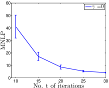
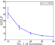
(a)	(b)
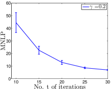
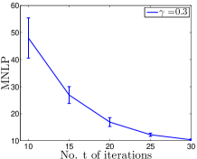
(c)	(d)

Figure 4: Graphs of MNLPs (with standard deviations) achieved by $s$VBSSGP vs. number $t$ of iterations with varying values of $\gamma$ for the AIMPEAK dataset.

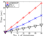
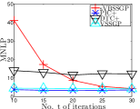
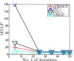
(a)	(b)	(c)

Figure 5: (a) Graph of total training time incurred by $s$VBSSGP, PIC$+$, and DTC$+$ vs. number $t$ of iterations for the AIMPEAK dataset; and graphs of MNLPs achieved by $s$VBSSGP, PIC$+$, DTC$+$, and VSSGP vs. number $t$ of iterations for the (b) AIMPEAK and (c) AIRLINE datasets.

References

- [Buza 2014] Buza, K. 2014. Feedback prediction for blogs. In Spiliopoulou, M.; Schmidt-Thieme, L.; and Janning, R., eds., Data Analysis, Machine Learning and Knowledge Discovery. Springer International Publishing. 145–152.
- [Cao, Low, and Dolan 2013] Cao, N.; Low, K. H.; and Dolan, J. M. 2013. Multi-robot informative path planning for active sensing of environmental phenomena: A tale of two algorithms. In Proc. AAMAS.
- [Chen et al. 2012] Chen, J.; Low, K. H.; Tan, C. K.-Y.; Oran, A.; Jaillet, P.; Dolan, J. M.; and Sukhatme, G. S. 2012. Decentralized data fusion and active sensing with mobile sensors for modeling and predicting spatiotemporal traffic phenomena. In Proc. UAI, 163–173.
- [Chen et al. 2013] Chen, J.; Cao, N.; Low, K. H.; Ouyang, R.; Tan, C. K.-Y.; and Jaillet, P. 2013. Parallel Gaussian process regression with low-rank covariance matrix approximations. In Proc. UAI, 152–161.
- [Chen et al. 2015] Chen, J.; Low, K. H.; Jaillet, P.; and Yao, Y. 2015. Gaussian process decentralized data fusion and active sensing for spatiotemporal traffic modeling and prediction in mobility-on-demand systems. IEEE T-ASE 12(3):901–921.
- [Chen, Low, and Tan 2013] Chen, J.; Low, K. H.; and Tan, C. K.-Y. 2013. Gaussian process-based decentralized data fusion and active sensing for mobility-on-demand system. In Proc. RSS.
- [Dolan et al. 2009] Dolan, J. M.; Podnar, G.; Stancliff, S.; Low, K. H.; Elfes, A.; Higinbotham, J.; Hosler, J. C.; Moisan, T. A.; and Moisan, J. 2009. Cooperative aquatic sensing using the telesupervised adaptive ocean sensor fleet. In Proc. SPIE Conference on Remote Sensing of the Ocean, Sea Ice, and Large Water Regions, volume 7473.
- [Gal and Turner 2015] Gal, Y., and Turner, R. 2015. Improving the Gaussian process sparse spectrum approximation by representing uncertainty in frequency inputs. In Proc. ICML, 655–664.
- [Hensman, Fusi, and Lawrence 2013] Hensman, J.; Fusi, N.; and Lawrence, N. D. 2013. Gaussian processes for big data. In Proc. UAI, 282–290.
- [Hoang et al. 2014a] Hoang, T. N.; Low, K. H.; Jaillet, P.; and Kankanhalli, M. 2014a. Active learning is planning: Nonmyopic -Bayes-optimal active learning of Gaussian processes. In Proc. ECML/PKDD Nectar Track, 494–498.
- [Hoang et al. 2014b] Hoang, T. N.; Low, K. H.; Jaillet, P.; and Kankanhalli, M. 2014b. Nonmyopic -Bayes-Optimal Active Learning of Gaussian Processes. In Proc. ICML, 739–747.
- [Hoang, Hoang, and Low 2015] Hoang, T. N.; Hoang, Q. M.; and Low, K. H. 2015. A unifying framework of anytime sparse Gaussian process regression models with stochastic variational inference for big data. In Proc. ICML, 569–578.
- [Hoang, Hoang, and Low 2016] Hoang, T. N.; Hoang, Q. M.; and Low, K. H. 2016. A distributed variational inference framework for unifying parallel sparse Gaussian process regression models. In Proc. ICML, 382–391.
- [Lázaro-Gredilla et al. 2010] Lázaro-Gredilla, M.; Quiñonero-Candela, J.; Rasmussen, C. E.; and Figueiras-Vidal, A. R. 2010. Sparse spectrum Gaussian process regression. JMLR 1865–1881.
- [Ling, Low, and Jaillet 2016] Ling, C. K.; Low, K. H.; and Jaillet, P. 2016. Gaussian process planning with Lipschitz continuous reward functions: Towards unifying Bayesian optimization, active learning, and beyond. In Proc. AAAI, 1860–1866.
- [Low et al. 2012] Low, K. H.; Chen, J.; Dolan, J. M.; Chien, S.; and Thompson, D. R. 2012. Decentralized active robotic exploration and mapping for probabilistic field classification in environmental sensing. In Proc. AAMAS, 105–112.
- [Low et al. 2014a] Low, K. H.; Chen, J.; Hoang, T. N.; Xu, N.; and Jaillet, P. 2014a. Recent advances in scaling up Gaussian process predictive models for large spatiotemporal data. In Proc. DyDESS.
- [Low et al. 2014b] Low, K. H.; Xu, N.; Chen, J.; Lim, K. K.; and Özgül, E. B. 2014b. Generalized online sparse Gaussian processes with application to persistent mobile robot localization. In Proc. ECML/PKDD Nectar Track, 499–503.
- [Low et al. 2015] Low, K. H.; Yu, J.; Chen, J.; and Jaillet, P. 2015. Parallel Gaussian process regression for big data: Low-rank representation meets Markov approximation. In Proc. AAAI.
- [Low, Dolan, and Khosla 2008] Low, K. H.; Dolan, J. M.; and Khosla, P. 2008. Adaptive multi-robot wide-area exploration and mapping. In Proc. AAMAS, 23–30.
- [Low, Dolan, and Khosla 2009] Low, K. H.; Dolan, J. M.; and Khosla, P. 2009. Information-theoretic approach to efficient adaptive path planning for mobile robotic environmental sensing. In Proc. ICAPS.
- [Low, Dolan, and Khosla 2011] Low, K. H.; Dolan, J. M.; and Khosla, P. 2011. Active Markov information-theoretic path planning for robotic environmental sensing. In Proc. AAMAS, 753–760.
- [Ouyang et al. 2014] Ouyang, R.; Low, K. H.; Chen, J.; and Jaillet, P. 2014. Multi-robot active sensing of non-stationary Gaussian process-based environmental phenomena. In Proc. AAMAS.
- [Podnar et al. 2010] Podnar, G.; Dolan, J. M.; Low, K. H.; and Elfes, A. 2010. Telesupervised remote surface water quality sensing. In Proc. IEEE Aerospace Conference.
- [Quiñonero-Candela and Rasmussen 2005] Quiñonero-Candela, J., and Rasmussen, C. E. 2005. A unifying view of sparse approximate Gaussian process regression. Journal of Machine Learning Research 6:1939–1959.
- [Titsias and Lázaro-Gredilla 2014] Titsias, M. K., and Lázaro-Gredilla, M. 2014. Doubly stochastic variational Bayes for non-conjugate inference. In Proc. ICML, 1971–1979.
- [Titsias 2009] Titsias, M. K. 2009. Variational learning of inducing variables in sparse Gaussian processes. In Proc. AISTATS.
- [Xu et al. 2014] Xu, N.; Low, K. H.; Chen, J.; Lim, K. K.; and Özgül, E. B. 2014. GP-Localize: Persistent mobile robot localization using online sparse Gaussian process observation model. In Proc. AAAI, 2585–2592.
- [Yu et al. 2012] Yu, J.; Low, K. H.; Oran, A.; and Jaillet, P. 2012. Hierarchical Bayesian nonparametric approach to modeling and learning the wisdom of crowds of urban traffic route planning agents. In Proc. IAT, 478–485.
- [Zhang et al. 2016] Zhang, Y.; Hoang, T. N.; Low, K. H.; and Kankanhalli, M. 2016. Near-optimal active learning of multi-output Gaussian processes. In Proc. AAAI, 2351–2357.