Controlling quark mass determinations non-perturbatively in three-flavour QCD

Abstract

The determination of quark masses from lattice QCD simulations requires a non-perturbative renormalization procedure and subsequent scale evolution to high energies, where a conversion to the commonly used $\kern 1.0pt\overline{\kern 0.0pt\rm MS\kern-1.0pt}\kern 1.0pt$ scheme can be safely established. We present our results for the non-perturbative running of renormalized quark masses in $N_{\rm f}=3$ QCD between the electroweak and a hadronic energy scale, where lattice simulations are at our disposal. Recent theoretical advances in combination with well-established techniques allows to follow the scale evolution to very high statistical accuracy, and full control of systematic effects.

1 Quantum Chromodynamics at all scales

For numerical simulations one starts from one of many valid discretisations of the (bare) Euclidean action density of Quantum Chromodynamics (QCD),

$$\mathcal{L}_{\tiny QCD} =\frac{1}{2g_{0}^{2}}\,\hbox{tr}\,\{F_{\mu\nu}F_{\mu\nu}\}+\sum_{i=1}^{N_{\rm f}}\overline{\psi}_{i}\big{(}\gamma_{\mu}D_{\mu}+m_{0,i}\big{)}\psi_{i}\;, D_{\mu} =\partial_{\mu}+A_{\mu}\;,$$ (1)

with a fixed number of dynamical quark flavours $N_{\rm f}$. With $N_{\rm f}+1$ input parameters the action is supposed to describe the strong interaction at all energy scales. Lattice QCD is a gauge-invariant regularisation and thus does not require a gauge-fixing and Faddeev–Popov term. It is the only regularisation allowing to determine colorless bound states $(m_{\tiny\pi^{0}},m_{\tiny\rm K^{0}},m_{\rm p},\ldots)$ between quarks from first principle calculations, which due to computational and theoretical advances can be systematically improved over time. However, incorporating all physical mass-scales that are relevant for describing ($N_{\rm f}=6$) QCD—as it seems to be realised in nature—is an impossible task to present state-of-the-art simulations due to the immense costs to accommodate many orders of magnitude of energy scales in a single simulation, cf. Figure 1. Being mainly interested in non-perturbative, long-distance effects of QCD, the phenomenological applicability of LQCD is limited to a fixed window

$$40\,{\rm MeV}\;\sim\;\Lambda_{\tiny\rm IR}\;\ll\;\mu_{\rm had},\,m_{\tiny\pi^{0}},\,m_{\rm p},\,m_{\tiny\rm K^{0}},\,\ldots\;\ll\;\Lambda_{\tiny\rm UV}\;\sim\;3\,{\rm GeV}\;.$$ (2)

Any physically interesting scale $\mu$ has to be well separated from the imposed infrared and ultraviolet cutoffs, $\Lambda_{\tiny\rm IR}\ll\mu\ll\Lambda_{\tiny\rm UV}$, to allow for a controlled assessment of the respective cutoff effects, see caption of Figure 1. Although, the lattice community can afford to simulate with three or four dynamical flavours nowadays, one still needs to balance the $N_{\rm f}+1$ chosen (bare) input parameters, given in terms of $N_{\rm f}+1$ physical scales from the real spectrum, against the intrinsic cutoff values and algorithmic costs. As no practical perfect lattice setup exists, different views on how to best achieve this balance lead to controversies among lattice practitioners. Another of those disputable topics is the application of perturbation theory at energies as low as those given by the low-energy window of lattice QCD as specified in (2), including $\mu=\Lambda_{\tiny\rm UV}\sim\,3\,{\rm GeV}$, see also Brida:2016flw .

In course of our determination of quark masses, we have to fix a renormalization prescription at scale $\mu_{\rm had}$ that lies well inside the window $[\Lambda_{\tiny\rm IR},\Lambda_{\tiny\rm UV}]$. Then the natural question arises how to compare or connect our result to other determinations as summarised for instance by the Particle Data Group PDG:2014 . Both naturally differ in the renormalization scheme and scale. After removing the UV cutoff dependence, we thus have to evolve our (continuum) result, $\kern 1.0pt\overline{\kern-1.0ptm\kern-1.0pt}\kern 1.0pt_{i}(\mu_{\rm had})$, using renormalization group (RG) transformations to the same physical scale and scheme, typically $\kern 1.0pt\overline{\kern 0.0pt\rm MS\kern-1.0pt}\kern 1.0pt$.

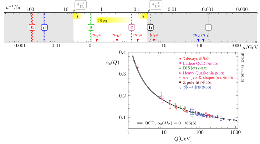
Figure 1: Sketch of energy scales relevant to QCD phenomenology. The masses for the six quark flavours found in nature so far (u, d, s, c, b, t) are taken as quoted in PDG:2014 . Also the masses of the neutral pseudoscalar meson bound states ($m_{\tiny\pi^{0}}$, $m_{\tiny\rm K^{0}}$, $m_{\tiny\rm D^{0}}$, $m_{\tiny\rm B^{0}}$) as well as the depicted scale dependence of the strong coupling $\alpha_{\rm s}$ are taken from that reference. Although, $\alpha_{\rm s}(\mu)$ can be computed in any sensible renormalization scheme one conveniently quotes it for the 5-flavour theory at the electroweak scale $\mu=m_{\tiny\rm Z}$ in the $\kern 1.0pt\overline{\kern 0.0pt\rm MS\kern-1.0pt}\kern 1.0pt$ scheme.
The lattice regularisation of QCD provides the only known (non-perturbative and gauge-invariant) framework to compute bound states of the strong interaction. For phenomenological applications one is restricted to a window ($\Lambda_{\rm IR}\leq\mu\leq\Lambda_{\rm UV}$) in the low-energy regime of QCD in order to incorporate the important long-distance effects. They are of the order of the Compton wavelength of the lightest particle, $\lambda_{\pi^{0}}=1/m_{\tiny\pi^{0}}$. It has to be well separated from the infrared cutoff $\Lambda_{\rm IR}^{-1}\sim L\gg\lambda_{\pi^{0}}$ in order to not be distorted by finite volume effects. Typical simulations have a physical extent of $L\gtrsim 3\,{\rm fm}$ and a number of lattice points of $N=(L/a)^{4}\approx(50-100)^{4}$, thus restricting the lattice spacing to $a\sim\Lambda_{\rm UV}^{-1}\gtrsim 0.045\,{\rm fm}$. To extract physical quantities one also has to stay away from the ultraviolet cutoff, i.e. $\mu\ll\Lambda_{\rm UV}$, otherwise control over finite lattice spacing effects is lost, and the continuum limit $a\to 0$ cannot be taken. Although, various advances in LQCD steadily increase the quality and reliability of numerical simulations with different number of flavours $N_{\rm f}$, the cost of simulations and algorithmic difficulties still prevent us from reaching even smaller lattice spacings.
For any non-perturbative renormalization problem posed at fixed renormalization scale $\mu$ in the low-energy regime of LQCD the continuum limit has to be taken in a controlled way. Then the remaining question is how to relate the obtained results to experiments at much higher energies, typically two orders of magnitude. For high precision physics the supposedly most convenient renormalization scheme, $\kern 1.0pt\overline{\kern 0.0pt\rm MS\kern-1.0pt}\kern 1.0pt$, is of little help at scales much below $10\,{\rm GeV}$ (or $\alpha_{\rm s}\gtrsim 0.2$). Its intrinsic perturbative nature, the behaviour of asymptotic series expansions in general, and missing non-perturbative contributions prevent us from quantifying its (non-)reliability at low energies from within the scheme itself. As detailed in the main text the renormalization group running of any operator can be determined purely non-perturbative, thus connecting the low-energy regime of LQCD in a controlled and quantifiable way to scales well above $10\,{\rm GeV}$. Recently, it has become possible to non-perturbatively test the accuracy of continuum perturbation theory for $\alpha_{\rm s}\lesssim 0.2$ Brida:2016flw , stressing the relevance and necessity of a careful assessment beyond perturbation theory in present high precision physics. Non-perturbatively it is even possible nowadays to follow the renormalization group in QCD down to scales of about $200\,{\rm MeV}$, cf. Ref. DallaBrida:2016kgh . Both results have been reported at this conference Sint:12Conf2016 ; DallaBrida:12Conf2016 .

In a mass-independent renormalization scheme for QCD, the renormalization group equations (RGE) for the running coupling and running quark mass(es) read

$$\mu\dfrac{\partial}{\partial\mu}\kern 1.0pt\overline{\kern-1.0ptg\kern-1.0pt}\kern 1.0pt(\mu) =\beta(\kern 1.0pt\overline{\kern-1.0ptg\kern-1.0pt}\kern 1.0pt)\;, \dfrac{\mu}{\kern 1.0pt\overline{\kern-1.0ptm\kern-1.0pt}\kern 1.0pt}\dfrac{\partial}{\partial\mu}\kern 1.0pt\overline{\kern-1.0ptm\kern-1.0pt}\kern 1.0pt(\mu) =\tau(\kern 1.0pt\overline{\kern-1.0ptg\kern-1.0pt}\kern 1.0pt)\;,$$ (3)

and can be formally integrated. The resulting, exact solutions are known as renormalization group invariants (RGI), conveniently written as

$${\Lambda} \equiv\mu\big{[}{b_{0}\kern 1.0pt\overline{\kern-1.0ptg\kern-1.0pt}\kern 1.0pt^{2}(\mu)}\big{]}^{-{b_{1}}/({2b_{0}^{2}})}\,{\rm e}^{-1/({2b_{0}\kern 1.0pt\overline{\kern-1.0ptg\kern-1.0pt}\kern 1.0pt^{2}(\mu)})}\exp\bigg{(}\!-\!\!\int_{0}^{\kern 1.0pt\overline{\kern-1.0ptg\kern-1.0pt}\kern 1.0pt^{\vphantom{A}}(\mu)}\!\!\!\!{\rm d}{g}\,\bigg{[}\dfrac{1}{\beta(g)}+\dfrac{1}{b_{0}g^{3}}-\dfrac{b_{1}}{b_{0}^{2}g}\bigg{]}\bigg{)}\;,$$ (4)

$${M_{i}} \equiv\kern 1.0pt\overline{\kern-1.0ptm\kern-1.0pt}\kern 1.0pt_{i}(\mu)\big{[}{2b_{0}\kern 1.0pt\overline{\kern-1.0ptg\kern-1.0pt}\kern 1.0pt^{2}(\mu)}\big{]}^{-{d_{0}}/({2b_{0}})}\,\exp\bigg{(}\!-\!\!\int_{0}^{\kern 1.0pt\overline{\kern-1.0ptg\kern-1.0pt}\kern 1.0pt^{\vphantom{A}}(\mu)}\!\!\!\!{\rm d}{g}\,\bigg{[}\dfrac{\tau(g)}{\beta(g)}-\dfrac{d_{0}}{b_{0}g}\bigg{]}\bigg{)}\;,\quad i\in\{\rm u,d,s,c,b,t\}\,.$$ (5)

Only the leading, universal (scheme-independent) coefficients $b_{0},b_{1},d_{0}$ of the perturbative expansions of the beta-function and mass-anomalous dimension,

$$\beta(g) \mathrel{\mathop{\sim}^{g\to 0}}-g^{3}({b_{0}}+{b_{1}}g^{2}+{b_{2}^{s}}g^{4}+\ldots)\;, \tau(g) \mathrel{\mathop{\sim}^{g\to 0}}-g^{2}({d_{0}}+{d_{1}^{s}}g^{2}+\ldots)\;,$$ (6)

appear such that the individual integrands are finite when $g\to 0$. Higher order coefficients are scheme-dependent—indicated by the superscript $s$—and so are $\beta$ and $\tau$. Thanks to recently completed efforts these approximations are now known to 5-loop order in the minimal subtraction scheme(s), cf. Gross:1973id ; Politzer:1973fx ; Caswell:1974gg ; Tarasov:1980au ; vanRitbergen:1997va ; Czakon:2004bu ; Baikov:2016tgj and Tarrach:1980up ; Tarasov:1982gk ; Chetyrkin:1997dh ; Vermaseren:1997fq ; Baikov:2014qja . However, it is well-known that by using an asymptotic series expansions one is missing non-perturbative contributions which become increasingly more relevant towards low energies, i.e., when the strong coupling becomes large. One has to appreciate that these issues can be overcome by determining $\beta(g)$ and $\tau(g)$ non-perturbatively. In that case, eqs. (4) and (5) determine the fundamental parameters $\{\Lambda,M_{i}\}_{N_{\rm f}}$ uniquely for any input scale $\mu$.

2 An intermediate non-perturbative renormalization scheme

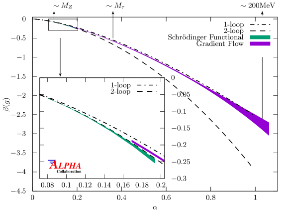
Figure 2: Non-perturbative $\beta$-function for the SF ($\alpha_{\rm SF}\lesssim 0.2$) and GF ($\alpha_{\rm GF}\gtrsim 0.17$) running coupling scheme; picture from DallaBrida:2016kgh . There also the two schemes have been matched non-perturbatively at fixed physical volume corresponding to about $4\,{\rm GeV}$.

For massless renormalization schemes (RS) it is most natural to first solve the RG equation for the coupling and then for the mass, cf. (3). In LQCD it has become customary to determine the scale evolution of coupling and mass using a finite-volume renormalization scheme in combination with recursive finite-size scaling. For that purpose the physical size $L$ of the simulated volume $L^{4}$ is identified with the inverse renormalization scale for the sole purpose of solving the RG equations by rescaling the box size, $L\to sL$. The constant factor $s$ is usually chosen to be $2$. In that way one is able to cleanly disentangle the renormalization procedure from the low-energy window of LQCD and to connect the hadronic renormalization scale $\mu_{\rm had}=1/L_{\rm had}$ to the electroweak scale $\mu=m_{\tiny\rm Z}$, where for instance a change of renormalization schemes towards the commonly quoted $\kern 1.0pt\overline{\kern 0.0pt\rm MS\kern-1.0pt}\kern 1.0pt$ scheme can typically be achieved in a controlled way, cf. Figure 1. For that purpose one should ideally cover a range of scales compatible with

$$L_{\rm max} \geq L_{\rm had}\;, L_{\rm min} \leq 1/m_{\tiny\rm Z}\;, L_{\rm max}/L_{\rm min} =s^{N_{s}}\;, s>1\;.$$ (7)

For example, to connect a scale $\mu_{\rm had}$ as low as $200\,{\rm MeV}$ to the electroweak scale of about $100\,{\rm GeV}$ using $s=2$, at least $N_{s}=9$ individual steps are necessary. Each of the $N_{s}$ steps requires a series of lattice simulations at different resolutions $L/a$ but fixed renormalized input parameters, $\kern 1.0pt\overline{\kern-1.0ptg\kern-1.0pt}\kern 1.0pt^{2}(L)=u$ and $L\kern 1.0pt\overline{\kern-1.0ptm\kern-1.0pt}\kern 1.0pt_{i}(L)=0$. In this way $\mu=1/L$ is kept fixed while only the lattice spacing $a$ is being varied, or equivalently, the bare parameters $\{g_{0}^{2},m_{0,i}\}$ as a function of $a$. A second set of simulations at the same bare parameters but $sL/a$ number of points in each direction permits to trace the change of renormalization scale $L\to sL$ at finite $a$. With adequate renormalization conditions for the coupling and quark mass, this allows to take the continuum limit $a\to 0$ of their lattice approximants in order to determine the response w.r.t. a change of scale $s$ in the continuum, equivalent to

$$-\ln(s) =\int^{\,\kern 1.0pt\overline{\kern-1.0ptg\kern-1.0pt}\kern 1.0pt(sL)}_{\,\kern 1.0pt\overline{\kern-1.0ptg\kern-1.0pt}\kern 1.0pt(L)}\!\!\frac{{\rm d}g}{\beta(g)}\;, \ln(\sigma_{\rm P}) =-\int^{\,\kern 1.0pt\overline{\kern-1.0ptg\kern-1.0pt}\kern 1.0pt(sL)}_{\,\kern 1.0pt\overline{\kern-1.0ptg\kern-1.0pt}\kern 1.0pt(L)}\!\!\!{\rm d}g\frac{\tau(g)}{\beta(g)}\;, \quad\begin{cases}\;\;\;\kern 1.0pt\overline{\kern-1.0ptg\kern-1.0pt}\kern 1.0pt^{2}(L)=u\\ \,L\kern 1.0pt\overline{\kern-1.0ptm\kern-1.0pt}\kern 1.0pt_{i}(L)=0\end{cases}\;.$$ for fixed (8)

In this way, the relevant information is encoded in the step-scaling functions (SSFs) Luscher:1993gh ; Capitani:1998mq ,

$$\sigma(s,u) =\kern 1.0pt\overline{\kern-1.0ptg\kern-1.0pt}\kern 1.0pt^{2}(sL)\;, \sigma_{\rm P}(s,u) =\kern 1.0pt\overline{\kern-1.0ptm\kern-1.0pt}\kern 1.0pt_{i}(L)\big{/}\kern 1.0pt\overline{\kern-1.0ptm\kern-1.0pt}\kern 1.0pt_{i}(sL)\;.$$ (9)

While various ways exist to determine the SSFs numerically via lattice simulations of QCD, the so-called Schrödinger functional (SF) setup Luscher:1992an ; Sint:1993un ; Sint:1995rb has been develop for exactly that purpose. For instance, in contrast to standard (anti-)periodic boundary conditions in all space time directions, Dirichlet boundary conditions are imposed in time direction. This allows for a natural non-perturbative definition of a strong coupling via non-vanishing boundary gauge fields as well as to simulate at vanishing quark mass. For additional details we point to the review article Sommer:2015kza and references therein.

The scale evolution of the strong coupling has been determined in refs. Brida:2016flw ; DallaBrida:2016kgh , and a short account of the whole procedure can be found in Bruno:2016gvs . However, a technical complication is inherited from that determination: instead of a single RS, two different schemes are being used and matched non-perturbatively at a scale of approx. $4\,{\rm GeV}$. At present, its physical motivation is two-fold: 1) control the perturbative matching at the electroweak scale to high precision Brida:2016flw using the Schrödinger functional coupling, $\kern 1.0pt\overline{\kern-1.0ptg\kern-1.0pt}\kern 1.0pt_{\rm SF}$, and 2) reach good statistical accuracy down to energies of about $200\,{\rm MeV}$ DallaBrida:2016kgh by applying the Gradient flow coupling scheme, $\kern 1.0pt\overline{\kern-1.0ptg\kern-1.0pt}\kern 1.0pt_{\rm GF}$ Fritzsch:2013je ; Ramos:2015baa . Compared to previous estimates of $\alpha_{\rm s}(m_{\tiny\rm Z})$ this represents a new quality of rigor from lattice QCD determinations and for the first time allowed to accurately determine the corresponding non-perturbative QCD $\beta$-functions, see Figure 2.

For our determination of the scale evolution of renormalized quark masses in three-flavour QCD, this does not pose any additional obstacles but only complicates the overall presentation. In fact, assuming a diagonal quark mass matrix of rank $N_{\rm f}$ in two massless schemes, one can write Sint:1998iq

$$\mu^{\prime} =c\mu\,,\;c>0, \kern 1.0pt\overline{\kern-1.0ptg\kern-1.0pt}\kern 1.0pt^{\prime 2} =\kern 1.0pt\overline{\kern-1.0ptg\kern-1.0pt}\kern 1.0pt^{2}{\cal X}_{\rm g}(\kern 1.0pt\overline{\kern-1.0ptg\kern-1.0pt}\kern 1.0pt)\,, \kern 1.0pt\overline{\kern-1.0ptm\kern-1.0pt}\kern 1.0pt_{j}^{\prime} =\kern 1.0pt\overline{\kern-1.0ptm\kern-1.0pt}\kern 1.0pt_{j}^{\vphantom{{}^{\prime}}}\,{\cal X}_{\rm m}^{\vphantom{{}^{\prime}}}(\kern 1.0pt\overline{\kern-1.0ptg\kern-1.0pt}\kern 1.0pt)\,, j=1,\ldots,N_{\rm f}\,.$$ (10)

Invariance of a physical observable $P$ under this change of variables implies

$$P^{\prime}\big{[}\,\mu^{\prime}(\mu),\,\kern 1.0pt\overline{\kern-1.0ptg\kern-1.0pt}\kern 1.0pt^{\prime}(\kern 1.0pt\overline{\kern-1.0ptg\kern-1.0pt}\kern 1.0pt),\,\{\kern 1.0pt\overline{\kern-1.0ptm\kern-1.0pt}\kern 1.0pt_{j}^{\prime}(\kern 1.0pt\overline{\kern-1.0ptg\kern-1.0pt}\kern 1.0pt,\kern 1.0pt\overline{\kern-1.0ptm\kern-1.0pt}\kern 1.0pt_{j}^{\vphantom{{}^{\prime}}})\}\,\big{]} =P\,\big{[}\,\mu,\,\kern 1.0pt\overline{\kern-1.0ptg\kern-1.0pt}\kern 1.0pt,\,\{\kern 1.0pt\overline{\kern-1.0ptm\kern-1.0pt}\kern 1.0pt_{j}\}\big{]}\;,$$ (11)

where $P^{\prime}$ satisfies the Callan–Symanzik equation in the primed scheme w.r.t.

$$\beta^{\prime}(\kern 1.0pt\overline{\kern-1.0ptg\kern-1.0pt}\kern 1.0pt^{\prime}) =\left\{\beta(\kern 1.0pt\overline{\kern-1.0ptg\kern-1.0pt}\kern 1.0pt)\frac{\partial\kern 1.0pt\overline{\kern-1.0ptg\kern-1.0pt}\kern 1.0pt^{\prime}}{\partial\kern 1.0pt\overline{\kern-1.0ptg\kern-1.0pt}\kern 1.0pt}\right\}_{\kern 1.0pt\overline{\kern-1.0ptg\kern-1.0pt}\kern 1.0pt=\kern 1.0pt\overline{\kern-1.0ptg\kern-1.0pt}\kern 1.0pt(\kern 1.0pt\overline{\kern-1.0ptg\kern-1.0pt}\kern 1.0pt^{\prime})}\;, \tau^{\prime}(\kern 1.0pt\overline{\kern-1.0ptg\kern-1.0pt}\kern 1.0pt^{\prime}) =\left\{\tau(\kern 1.0pt\overline{\kern-1.0ptg\kern-1.0pt}\kern 1.0pt)+\beta(\kern 1.0pt\overline{\kern-1.0ptg\kern-1.0pt}\kern 1.0pt)\frac{\partial}{\partial\kern 1.0pt\overline{\kern-1.0ptg\kern-1.0pt}\kern 1.0pt}\ln{\cal X}_{\rm m}(\kern 1.0pt\overline{\kern-1.0ptg\kern-1.0pt}\kern 1.0pt)\right\}_{\kern 1.0pt\overline{\kern-1.0ptg\kern-1.0pt}\kern 1.0pt=\kern 1.0pt\overline{\kern-1.0ptg\kern-1.0pt}\kern 1.0pt(\kern 1.0pt\overline{\kern-1.0ptg\kern-1.0pt}\kern 1.0pt^{\prime})}\;.$$ (12)

While this is the general connection between two massless schemes at the level of RG functions, every step in our determination is done non-perturbatively. In practise, when switching between the two schemes, we do not change the imposed renormalization condition—which is relevant for determining $\sigma_{\rm P}(2,u)$—but merely the implicit, parametric dependence on the renormalized coupling $u\equiv\kern 1.0pt\overline{\kern-1.0ptg\kern-1.0pt}\kern 1.0pt^{2}(L)$. The connection between SF and GF schemes has been established non-perturbatively at a well-chosen fixed physical box size, $L_{0}\approx(4\,{\rm GeV})^{-1}$, and reads DallaBrida:2016kgh

$$\kern 1.0pt\overline{\kern-1.0ptg\kern-1.0pt}\kern 1.0pt_{\rm SF}^{2}(L_{0}) =2.012\;, \kern 1.0pt\overline{\kern-1.0ptg\kern-1.0pt}\kern 1.0pt_{\rm GF}^{2}(2L_{0}) =2.6723(64)\;.$$ (13)

3 The running quark mass

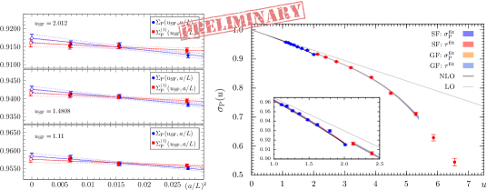
Figure 3: Left: Representative continuum extrapolations ($u$-by-$u$) for the step-scaling function $\sigma_{\rm P}(u)\equiv\lim_{a/L\to 0}\Sigma^{(1)}(u,a/L)$ in the SF scheme. For further details please consult Campos:2015fka ; Lattice16 . Right: Non-perturbatively determined step-scaling functions $\sigma_{\rm P}(u)$ in the SF ($u\lesssim 2.0$) and GF ($u\gtrsim 2.1$) running coupling scheme, together with different interpolating fits. We note that for $u_{\rm SF}\lesssim 1.5$ the data agrees with NLO perturbation theory such that the matching with SF-PT can be safely established.

Given the discussions in the previous sections, our strategy of a non-perturbatively controlled determination of quark masses in the three-flavour theory with two renormalization schemes proceeds as follows. We determine the flavour-independent RG factor ${M}/{\kern 1.0pt\overline{\kern-1.0ptm\kern-1.0pt}\kern 1.0pt(\mu_{\rm had})}$, cf. eq. (5), that connects the RGI mass to the quark mass in the hadronic, low-energy regime

$$\frac{M}{\kern 1.0pt\overline{\kern-1.0ptm\kern-1.0pt}\kern 1.0pt(\mu_{\rm had})} =\left[\frac{\kern 1.0pt\overline{\kern-1.0ptm\kern-1.0pt}\kern 1.0pt(\mu_{\rm swi})}{\kern 1.0pt\overline{\kern-1.0ptm\kern-1.0pt}\kern 1.0pt(\mu_{\rm had})}\right]_{\rm GF-NP}\!\!\times\;\left[\frac{\kern 1.0pt\overline{\kern-1.0ptm\kern-1.0pt}\kern 1.0pt(\mu_{\rm PT})}{\kern 1.0pt\overline{\kern-1.0ptm\kern-1.0pt}\kern 1.0pt(\mu_{\rm swi})}\right]_{\rm SF-NP}\!\!\times\;\left[\frac{M}{\kern 1.0pt\overline{\kern-1.0ptm\kern-1.0pt}\kern 1.0pt(\mu_{\rm PT})}\right]_{\rm SF-PT}\;.$$ (14)

Note that we intend to make use of perturbation theory at a scale $\mu_{\rm PT}$ close to $m_{\tiny\rm Z}$ where truncation errors from using the known 3-/2-loop orders in the perturbative $\beta$-/$\tau$-functions in the SF scheme are sufficiently suppressed, see Figure 3. The true challenge is to determine the two non-perturbative factors to a sufficient precision while controlling systematic effects at the sub-percent level for each individual contribution. When this is achieved, the scale- and scheme-independent RGI mass of flavour $j$ can be determined from

$$M_{j} =\frac{M}{\kern 1.0pt\overline{\kern-1.0ptm\kern-1.0pt}\kern 1.0pt(\mu_{\rm had})}\times\kern 1.0pt\overline{\kern-1.0ptm\kern-1.0pt}\kern 1.0pt_{j}(\mu_{\rm had})\;,$$ (15)

where $\kern 1.0pt\overline{\kern-1.0ptm\kern-1.0pt}\kern 1.0pt_{j}(\mu_{\rm had})$ constitutes a renormalized quark mass computed in the hadronic regime. Ideally, $M_{j}$ is the fundamental parameter to be compared to other determinations. However, it has become customary to quote $\kern 1.0pt\overline{\kern 0.0pt\rm MS\kern-1.0pt}\kern 1.0pt$ masses. In order to do so one subsequently has to employ perturbation theory and, depending on the individual flavour and renormalization scale, appropriately match at the charm and bottom thresholds.

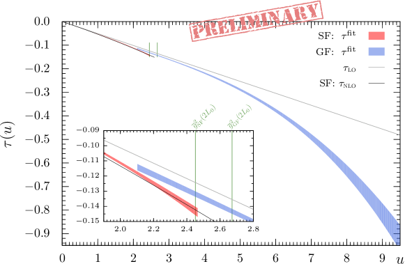
Figure 4: Non-perturbative mass anomalous dimension $\tau(g^{2})$ in the SF ($\kern 1.0pt\overline{\kern-1.0ptg\kern-1.0pt}\kern 1.0pt^{2}_{\rm SF}\lesssim 2.45$) and GF ($\kern 1.0pt\overline{\kern-1.0ptg\kern-1.0pt}\kern 1.0pt^{2}_{\rm GF}\gtrsim 2.10$) running coupling scheme. The vertical lines in the inner plot represent the respective couplings at the switching scale. Note that for $u=\kern 1.0pt\overline{\kern-1.0ptg\kern-1.0pt}\kern 1.0pt_{\rm GF}^{2}$ our data exactly covers the plotted fit range.

An important fact worth emphasising is that the continuum running factor in eq. (14) can be used by other lattice practitioners which may employ a different lattice discretization in their computations. They just have to recompute $\kern 1.0pt\overline{\kern-1.0ptm\kern-1.0pt}\kern 1.0pt_{j}(\mu_{\rm had})$ using the same—but so far unmentioned—renormalization prescription, such that eq. (15) remains well-defined. For the employed Wilson fermion action, the quark mass $\kern 1.0pt\overline{\kern-1.0ptm\kern-1.0pt}\kern 1.0pt_{j}$ can be obtained, on the lattice up to a finite renormalization, from the non-singlet axial Ward identity, or current quark mass

$$\kern 1.0pt\overline{\kern-1.0ptm\kern-1.0pt}\kern 1.0pt_{j}^{\rm\tiny awi}(\mu) =\lim_{a/L\to 0}\left[\frac{{Z_{\rm A}}(g_{0}^{2})}{{Z_{\rm P}}(g_{0}^{2},a\mu)}m_{j}^{\rm\tiny awi}\right]_{\mu=L^{-1}}\;, \partial_{\mu}\left[\overline{\psi}_{j}\gamma_{\mu}\gamma_{5}\psi_{j^{\prime}}(x)\right] =(m_{j}^{\rm\tiny awi}+m_{j^{\prime}}^{\rm\tiny awi})\,\overline{\psi}_{j}(x)\gamma_{5}\psi_{j^{\prime}}(x)\;.$$ (16)

The bare mass $m_{j}^{\rm\tiny awi}\equiv m_{j}^{\rm\tiny awi}(g_{0}^{2},\{am_{0,i}\})$ still depends on the bare parameters of the action, cf. eq. (1). From the previous discussions the connection to the mass-SSF and notation should become evident

$$\sigma_{\rm P}(s,u)\equiv\frac{\kern 1.0pt\overline{\kern-1.0ptm\kern-1.0pt}\kern 1.0pt_{j}^{\rm\tiny awi}(L)}{\kern 1.0pt\overline{\kern-1.0ptm\kern-1.0pt}\kern 1.0pt_{j}^{\rm\tiny awi}(sL)} =\lim_{a/L\to 0}\left[\frac{{Z_{\rm P}}(g_{0}^{2},sL/a)}{{Z_{\rm P}}(g_{0}^{2},L/a)}\right]_{\kern 1.0pt\overline{\kern-1.0ptg\kern-1.0pt}\kern 1.0pt^{2}(L)=u,m=0}\;,$$ (17)

cf. eqs. (8) and (9). ${Z_{\rm P}}$ is the multiplicative renormalization factor of the non-singlet pseudoscalar current, which itself is determined from a SF renormalization condition as in Capitani:1998mq .

In Figure 3 (left panel) we show preliminary results for some continuum extrapolations as in eq. (17) with $s=2$. The corresponding continuum SSF data points are then plotted against the initially fixed target couplings $u$ for both the SF- and GF-coupling schemes (right panel). Note that these values of $u$ can be chosen at will but should cover the range of interest well enough in order to reach the desired precision. Typical fit ansaetze as shown in Fig. 3 are polynomials like $\sigma_{\rm P}(u)=1+p_{\rm LO}u+p_{2}u^{2}+\cdots$ or Padé approximants with the correct, leading (universal) asymptotics fixed. With such a given smooth interpolation formula one is then able to recursively construct the running factor and its uncertainty in steps of $s=2$ as summarised in (7), i.e., the two ratios in (14) become

$$\frac{\kern 1.0pt\overline{\kern-1.0ptm\kern-1.0pt}\kern 1.0pt(\mu_{a})}{\kern 1.0pt\overline{\kern-1.0ptm\kern-1.0pt}\kern 1.0pt(\mu_{b})} =\prod_{k=1}^{N_{s}}\sigma_{\rm P}(u_{k})\;, \begin{cases}u_{k+1}=\sigma(u_{k})\\ u_{1}\quad\!=\kern 1.0pt\overline{\kern-1.0ptg\kern-1.0pt}\kern 1.0pt^{2}(\mu_{a})\\ \end{cases}\!\!\!\!, s_{ab} \equiv\frac{\mu_{a}}{\mu_{b}}=\frac{L_{b}}{L_{a}}=2^{N_{s}}\;.$$ (18)

Accordingly, we can identify the switching scale $L_{\rm swi}$ appearing in eq. (14) with the scale $2L_{0}$ of (13), which we inherit together with the coupling-SSF $\sigma(u)$ from the complementary determination of the running coupling Brida:2016flw ; DallaBrida:2016kgh ; Bruno:2016gvs ; DallaBrida:12Conf2016 ; Sint:12Conf2016 . This concludes the computation of (14) and we return to the determination of eq. (15), which we can now rewrite as

$$M_{j} =\frac{M}{\kern 1.0pt\overline{\kern-1.0ptm\kern-1.0pt}\kern 1.0pt(\mu_{\rm had})}\times\lim_{a/L\to 0}\left[\frac{{Z_{\rm A}}(g_{0}^{2})}{{Z_{\rm P}}(g_{0}^{2},a\mu_{\rm had})}m_{j}^{\rm\tiny awi}\right]\equiv\lim_{a/L\to 0}\left[{Z_{\rm M}}(g_{0}^{2})\,m_{j}^{\rm\tiny awi}(g_{0}^{2},\{am_{0,i}\})\right]\;.$$ (19)

The disappearance of the hadronic scale $\mu_{\rm had}$ reflects the scale-independence of $M_{j}$, which itself is connected to the current quark mass $m_{j}^{\rm\tiny awi}$ only by a scale-independent renormalization ${Z_{\rm M}}$. Hence, by determining ${Z_{\rm M}}$ the renormalization problem is fully solved non-perturbatively using the massless (intermediate) SF scheme. While the costs of simulating the Schrödinger functional setup are good to control in general, towards larger physical volumes the simulations get more and more involved and thus set a natural limit on the values the hadronic scale can take. At the moment we are exploring different ways to fix the value of $a\mu_{\rm had}$ in order to determine the ${Z_{\rm P}}(g_{0}^{2},a\mu_{\rm had})$, and thus ${Z_{\rm M}}$, with high precision.
As the reader may have noticed, forcing $s_{ab}$ in eq. (18) to be a multiple of $2$ is a quite stringent condition, especially as we already had to fix the scheme-switching scale in (14). Thanks to the high statistical accuracy and the achieved control of a few systematic effects which are propagated into the final error, we are able to lift this restriction for the first time. By reassessing eqs. (8) and (9), one notices that with the data points at hand and a given parameterisation of the $\beta$-function, as shown in Figure 2 and taken from Brida:2016flw ; DallaBrida:2016kgh , only a well motivated ansatz for $\tau(g)$ is required for a sensible least square minimisation. We present a preliminary but already very encouraging result in Figure 4, again for both the SF- and GF-running coupling schemes. It should be noted that this result is actually independent of the originally chosen scale-change factor $s=2$. As a non-trivial cross-check we can use the resultant to numerically reconstruct $\sigma_{\rm P}(u)$ for arbitrary $u$ from eq. (8). This is shown in Figure 3 and coincides very well with the original estimate. At the time of this conference we were still accumulating statistics at the two strongest renormalized couplings in use. Now we are finalising our analysis by also employing global fit ansaetze in various ways and include some yet missing correlations between our data, which is going to be published soon. Accordingly, we here refrain from quoting any quantitative numbers.

Compared to the aforementioned simulations, the $m_{j}^{\rm\tiny awi}$ estimates in (19) are obtained from large-scale lattice simulations that define the accessible low-energy window in the first place. We will employ $N_{\rm f}=2+1$ ensembles jointly produced by the Coordinated Lattice Simulations (CLS) effort Bruno:2014jqa , with which we share the lattice discretization in use. Although there have been many advances in lattice QCD, the accessible parameters $am_{0,i}$, in general, do not correspond directly to the set of parameters at which $m_{\pi}$ and $m_{\rm K}$ take their physical values for different values of the cutoffs (even after correcting for isospin splitting and QED effects). Beside setting the physical scale Bruno:2016plf , one thus still has to apply chiral perturbation theory. In that respect, eq. (19) is a minor simplification in our discussion, but nevertheless a step that has to be carefully evaluated in the near future.

4 Conclusions

We have presented a full strategy to determine renormalized quark masses from first principle lattice calculations in three-flavour QCD. Compared to other approaches in the community, we separate and thus disentangle the problem of renormalization from large-scale lattice QCD simulations. In this way the massless renormalization group running for the coupling and quark masses could be mapped out non-perturbatively to high accuracy in the employed Schrödinger functional scheme, and a connection to other schemes can be easily established via renormalization group invariant quantities $\{\Lambda,M_{i}\}_{N_{\rm f}}$. This strategy fully circumvents the unanswerable question regarding the applicability of perturbation theory at parametrically large values of the strong coupling. Furthermore, it provides a quantifiable and systematically improvable uncertainty at each stage of the calculation, something perturbation theory cannot really provide.

For the first time two different non-perturbative schemes, based on the Schrödinger functional coupling and the younger Gradient flow coupling, have been used and matched non-perturbatively. This specific combination has been chosen for the avail of improving on statistical and systematic uncertainties. Also the non-perturbative determination of the continuum quark mass anomalous dimension is a unique achievement for QCD.

The prospects for determining fundamental parameters of QCD valuable for high precision physics are excellent. To obtain an even more realistic approximation of nature this study can be extended to cross the charm flavour threshold $(N_{\rm f}=3\to N_{\rm f}=4)$ non-perturbatively at some point in the future. We finally remark that also the renormalization and scale dependence of the tensor current—relevant in rare meson decays (especially B decays), and studies of the neutron electric dipole moment—is being computed along the same lines Fritzsch:2015lvo .

References

- (1) M. Dalla Brida, P. Fritzsch, T. Korzec, A. Ramos, S. Sint, R. Sommer (ALPHA), Phys. Rev. Lett. 117, 182001 (2016), 1604.06193
- (2) K. Olive et al. (Particle Data Group), Chinese Physics C 38, 090001 (2014)
- (3) M. Dalla Brida, P. Fritzsch, T. Korzec, A. Ramos, S. Sint, R. Sommer (ALPHA) (2016), 1607.06423
- (4) S. Sint (ALPHA), EPJ Web of Conferences CONF12 (2016), this conference
- (5) M. Dalla Brida (ALPHA), EPJ Web of Conferences CONF12 (2016), this conference
- (6) D.J. Gross, F. Wilczek, Phys.Rev.Lett. 30, 1343 (1973)
- (7) H.D. Politzer, Phys.Rev.Lett. 30, 1346 (1973)
- (8) W.E. Caswell, Phys.Rev.Lett. 33, 244 (1974)
- (9) O. Tarasov, A. Vladimirov, A.Y. Zharkov, Phys.Lett. B93, 429 (1980)
- (10) T. van Ritbergen, J. Vermaseren, S. Larin, Phys.Lett. B400, 379 (1997), hep-ph/9701390
- (11) M. Czakon, Nucl.Phys. B710, 485 (2005), hep-ph/0411261
- (12) P.A. Baikov, K.G. Chetyrkin, J.H. KÃhn (2016), 1606.08659
- (13) R. Tarrach, Nucl.Phys. B183, 384 (1981)
- (14) O.V. Tarasov (1982), in Russian, preprint JINR P2-82-900
- (15) K. Chetyrkin, Phys.Lett. B404, 161 (1997), hep-ph/9703278
- (16) J. Vermaseren, S. Larin, T. van Ritbergen, Phys.Lett. B405, 327 (1997), hep-ph/9703284
- (17) P.A. Baikov, K.G. Chetyrkin, J.H. KÃhn, JHEP 10, 076 (2014), 1402.6611
- (18) M. Lüscher, R. Sommer, P. Weisz, U. Wolff, Nucl.Phys. B413, 481 (1994), hep-lat/9309005
- (19) S. Capitani, M. Lüscher, R. Sommer, H. Wittig (ALPHA), Nucl.Phys. B544, 669 (1999), hep-lat/9810063
- (20) M. Lüscher, R. Narayanan, P. Weisz, U. Wolff, Nucl.Phys. B384, 168 (1992), hep-lat/9207009
- (21) S. Sint, Nucl.Phys. B421, 135 (1994), hep-lat/9312079
- (22) S. Sint, Nucl.Phys. B451, 416 (1995), hep-lat/9504005
- (23) R. Sommer, U. Wolff (ALPHA), Nucl.Part.Phys.Proc. 261-262, 155 (2015), 1501.01861
- (24) M. Bruno et al. (ALPHA), The determination of by the ALPHA collaboration, in Proceedings, 6th Workshop on Theory, Phenomenology and Experiments in Flavour Physics : Interplay of Flavour Physics with electroweak symmetry breaking. (Capri 2016): Anacapri, Capri, Italy, June 11-13, 2016 (2017), Vol. 285-286, pp. 132–138, 1611.05750
- (25) P. Fritzsch, A. Ramos, JHEP 1310, 008 (2013), 1301.4388
- (26) A. Ramos, S. Sint, Eur. Phys. J. C76, 15 (2016), 1508.05552
- (27) S. Sint, P. Weisz (ALPHA), Nucl.Phys. B545, 529 (1999), hep-lat/9808013
- (28) I. Campos et al., PoS LATTICE2015, 249 (2016), 1508.06939
- (29) I. Campos et al., PoS LATTICE2016, 210 (2016)
- (30) M. Bruno et al., JHEP 1502, 043 (2015), 1411.3982
- (31) M. Bruno, T. Korzec, S. Schaefer (2016), 1608.08900
- (32) P. Fritzsch, C. Pena, D. Preti, PoS LATTICE2015, 250 (2016), 1511.05024