Diffusion of Active Particles With Stochastic Torques Modeled as $\alpha$-Stable Noise

Abstract

We investigate the stochastic dynamics of an active particle moving at a constant speed under the influence of a fluctuating torque. In our model the angular velocity is generated by a constant torque and random fluctuations described as a Lévy-stable noise. Two situations are investigated. First, we study white Lévy noise where the constant speed and the angular noise generate a persistent motion characterized by the persistence time $\tau_{D}$. At this time scale the crossover from ballistic to normal diffusive behavior is observed. The corresponding diffusion coefficient can be obtained analytically for the whole class of symmetric $\alpha$-stable noises. As typical for models with noise-driven angular dynamics, the diffusion coefficient depends non-monotonously on the angular noise intensity. As second example, we study angular noise as described by an Ornstein-Uhlenbeck process with correlation time $\tau_{c}$ driven by the Cauchy white noise. We discuss the asymptotic diffusive properties of this model and obtain the same analytical expression for the diffusion coefficient as in the first case which is thus independent on $\tau_{c}$. Remarkably, for $\tau_{c}>\tau_{D}$ the crossover from a non-Gaussian to a Gaussian distribution of displacements takes place at a time $\tau_{G}$ which can be considerably larger than the persistence time $\tau_{D}$.

I Introduction

Over the past few years an increasing interest to the motion of living organisms of different size and complexity (movement ecology Natan ) has lead to a large number of new experiments, some of them based on quite elaborated tools, allowing for study of this motion and for description of its observed trajectories. Examples are the works on dicstyostelium Bodecker , also under influence of chemotactic stimulus Anselem , on human motile keratinocytes and fibroblasts Selmeczi , on motile pieces of physarum Rodiek , on flagellate eukaryotes (Euglena) Euglena , also in time dependent light fields Romensky , and on more complex organisms as gastropods Seuront , zooplankton Ordemann , birds Edwards and zebra-tail fish Gautrais . One has also considered motion in the presence of boundaries which might substantially change its effective properties TefLow08 ; TefLo09 . Similar conceptual approaches were used to describe the motion of non-living motile objects, so called self-propelled particles, exhibiting similar trajectories He ; Takagi ; Hagen .

Theoretical modeling of self-motile objects goes back to the beginning of the last century Pearson ; Fuerth . Trajectories often appear to be stochastic Berg ; Campos ; Romanczuk , thus special attention has been paid to the development of different stochastic models for various physical or biological situations. These investigations yielded a great variety of possible mathematical models for the description of motion of self-propelled objects. Examples are the discrete hopping with a given turning angle distribution lsgzigzag ; HaLsg08 , the run and tumble model Thiel with polynomial waiting time densities exhibiting superdiffusive behavior etc. In order to determine the respective mean squared displacement (MSD) of the diffusive motion Langevin equations with associated kinetic equations for the probability densities have been introduced to describe propulsive motion under influence of noise sources, as modeled by white Gaussian noise Mikhailov ; Blum ; Peruani , by Gaussian Ornstein Uhlenbeck process Motsch ; Weber , or by dichotomic Markovian process Weber_Sok . Escape rates of active particles Burada , of active particles in external fields Ebeling ; Geiseler and active transport in cells Godec have been studied as well. Crawling patterns of Drosophila larvae motion where analyzed in Gunther by using a bimodal persistent random walk model. Here, the four parameters of the corresponding model were proved to be distinct for larvae with specific genetic mutations. This work elucidates the usefulness of elaborate, multiparametric models.

The origin of stochasticity, i.e. the nature of the noise sources, might be quite different, e.g. they may be due to neuronal activity, or due to interactions with the environment or with neighbors. The patchiness of the distribution of prey Edwards can be also considered as a noise source. There is still a debate on how to correctly describe various patterns of animal motion Reynolds . In the present work we extend the model of an active particle moving at a constant speed with a stochastic angular dynamics Weber to a more general case, when the random torques are described by an $\alpha$-stable noise. These Lévy or $\alpha$-stable noise sources lead to a directed motion interrupted by large jumps in the angle of orientation Dybiec . The sudden changes in the direction of movement and also the longer periods of curling appearing in this model might remind in particular the run and tumble processes Thiel .

In what follows we discuss two different angular dynamics. In the first case, Sec. II, we consider the motion in the presence of a constant torque and of a source of a symmetric $\alpha$-stable white noise. Afterwards, in Sec. III, we look at a non-white noise as generated by an Ornstein-Uhlenbeck process (OUP) driven by a Cauchy noise source. For both dynamics we derive the analytical expressions for the mean squared displacement (MSD) and for the effective diffusion coefficient, and discuss the crossover from the ballistic motion to normal diffusion in coordinate space. We show that the MSD, the diffusion coefficient, and the crossover time do not depend on the correlations in the noise source.

Recently, experiments on beads diffusing on macromolecules were performed Wang ; Wangnat and caught attention. In these experiments single particle tracking was used to follow the trajectories of the beads. The beads performed (passive) Fickian diffusion, but a non-Gaussian distribution of displacements was observed. These observations point out the necessity to pay special attention to the moments of the displacement distributions higher than the MSD. In our model indeed, at difference to the behavior of the MSD, the higher moments of the displacement are sensitive to correlations. In particular, in the diffusive regime of the OUP-driven active particles we find an exponential distribution of displacements at short time lags while at longer time lags this distribution tends to a Gaussian, an observation similar to the one reported by Wang et al. Wang ; Wangnat . In our case this effect is caused by correlations in the noise which create an additional persistence in the motion. The crossover time after which the Gaussian distribution is established depends strongly on these correlations.

II Torque and white $\alpha$-stable angular noise

The the time evolution of the position vector $\vec{r}=\left(x(t),y(t)\right)$ of the particle is described by the following set of equations:

$$\frac{\text{d}\vec{r}}{\text{d}t}=v_{0}\begin{pmatrix}\cos\varphi(t)\\ \sin\varphi(t)\end{pmatrix}$$ (1)

$$\frac{\text{d}\varphi}{\text{d}t}=\Omega+\frac{\sigma}{v_{0}}\xi(t)$$ (2)

where the angle $\varphi(t)$ gives the orientation of the velocity vector whose absolute value is $v_{0}$. $\Omega$ is a constant torque. The noise $\xi(t)$ considered here is a $\alpha$-stable noise. According to Ditlevsen Ditlevsen and Schertzer Schertzer , the associated Fokker-Planck-Equation for such a system is given by:

$$\frac{\partial}{\partial t}P(\varphi,t)=-\Omega\frac{\partial}{\partial\varphi}P+\frac{\sigma^{\alpha}}{v_{0}^{\alpha}}\frac{\partial^{\alpha}}{\partial|\varphi|^{\alpha}}P(\varphi,t).$$ (3)

Herein

$$\frac{\partial^{\alpha}}{\partial|\varphi|^{\alpha}}P(\varphi)=-\frac{1}{2\pi}\int_{-\infty}^{\infty}dke^{-ik\varphi}|k|^{\alpha}P(k)$$ (4)

stands for the $\alpha$-th symmetric Riesz-Weyl fractional derivative. The case $\alpha=2$ corresponds to a Gaussian white noise. The parameter $\alpha$ controls the sudden large changes in the velocity orientation. For lower values of $\alpha$ the noise distribution becomes sharper around the center and the tails become more pronounced, so that the probability of large sudden changes in $\varphi$ increases, while small changes become less likely.

The conditional probability density of the orientation $\varphi$ at time $t$, given the initial angle $\varphi_{0}$ at time $t_{0}$ of the velocity vector is given by the following expression Schertzer :

$$P(\varphi,t|\varphi_{0},t_{0})=\frac{1}{2\pi}\int_{-\infty}^{\infty}dke^{-ik(\varphi-\varphi_{0})}e^{ik\Omega(t-t_{0})}e^{-\left(\frac{\sigma}{v_{0}}|k|\right)^{\alpha}(t-t_{0})}.$$ (5)

In the following we will set the initial values to $t_{0}=0$ and $\varphi_{0}=0$. With the help of Eq.(5) the MSD for this dynamics can be easily calculated using the Green-Kubo relation. For simplicity of notation, we move the origin of the coordinate system to the initial position of the particle at time $t_{0}$. Hence we have as as initial values $\vec{r}_{0}=0$ or $x_{0}=x(t_{0})=0$ and $y_{0}=y(t_{0})=0$, if not explicitly defined otherwise. We assign $r(t)=|\vec{r}|=\sqrt{x^{2}(t)+y^{2}(t)}$. The MSD becomes:

$$\langle r^{2}(t)\rangle=2v_{0}^{2}t\int_{0}^{t}d\tau\left(1-\frac{\tau}{t}\right)\cos(\Omega\tau)e^{-\left(\frac{\sigma}{v_{0}}\right)^{\alpha}\tau}.$$ (6)

Introducing $\gamma=\left(\frac{\sigma}{v_{0}}\right)^{\alpha}$ and $a=\Omega^{2}+\gamma^{2}$ leads to the following form of the MSD:

$$\langle r^{2}(t)\rangle=2v_{0}^{2}\left(\frac{\gamma t}{a}+\frac{\left(\gamma^{2}-\Omega^{2}\right)\left(\cos(\Omega t)e^{-\gamma t}-1\right)-2\gamma\Omega\sin(\Omega t)e^{-\gamma t}}{a^{2}}\right).$$ (7)

For short times $t$ the MSD shows ballistic behavior, i.e. $\langle r^{2}(t)\rangle=v_{0}^{2}t^{2}$. For times $t\gg\tau_{D}$ with

$$\tau_{D}=\left(\frac{v_{0}}{\sigma}\right)^{\alpha}$$ (8)

being the crossover time, the motion becomes diffusive. The persistence length of the motion is

$$l_{D}=v_{0}\tau_{D}=v_{0}\left(\frac{v_{0}}{\sigma}\right)^{\alpha}$$ (9)

and by that dependent on the noise type through the parameter $\alpha$. The effective diffusion coefficient $D_{\text{eff}}$ is given by

$$D_{\text{eff}}=\lim\limits_{t\to\infty}\frac{\langle r^{2}(t)\rangle}{4t}=v_{0}^{2}\frac{\left(\frac{\sigma}{v_{0}}\right)^{\alpha}}{2\left(\Omega^{2}+\left(\frac{\sigma}{v_{0}}\right)^{2\alpha}\right)}.$$ (10)

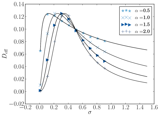
Figure 1: The effective diffusion coefficient $D_{\text{eff}}$ as a function of the parameters of the noise: Simulation (symbols) and theory (curves) for $\Omega=0.5$.

In the case of Gaussian white noise $(\alpha=2)$ the result of Weber et al.Weber is recovered. For $\Omega=0$ the effective diffusion coefficient $D_{\text{eff}}=v_{0}^{2+\alpha}/(2\sigma^{\alpha})$ decays with the growth of the scale parameter $\sigma$ as a power law, with a power given by the index of the Lévy distribution. Using Eq.(9) we see that the effective diffusion coefficients becomes $D_{\text{eff}}=v_{0}l_{D}/2$.

In Fig.1 we show the effective diffusion coefficient $D_{\text{eff}}$ for various values of $\alpha$ and non-zero torque, as obtained in simulations and from (Eq.(10)). The effective diffusion coefficient always shows a maximum at $\sigma_{\text{max}}=v\Omega^{1/\alpha}$, where it is equal to $D_{\text{eff}}^{\text{max}}=v_{0}^{2}/(4\Omega)$. This maximal value of the diffusion coefficient does not depend on the properties of the noise. For $\Omega\neq 0$ the diffusion coefficient vanishes for $\sigma\rightarrow 0$ and for $\sigma\rightarrow\infty$. How fast it vanishes depends on $\alpha$. The higher the value of $\alpha$ the smaller becomes the width of the peak. All curves intersect at $\sigma=v_{0}$. One also notices that the diffusion for $\alpha<2$ for a given $\sigma$ can be both faster or slower than in the Gaussian case. For small noise intensities the motion of the particle is dominated by the torque, the particle moves in circles and the diffusion is slow. Increasing the noise stretches the trajectories till the diffusion reaches the maximum. Behind the maximum the motion becomes noise-dominated, and the diffusion coefficient falls again.

Simulations show that for times $t$ larger than the crossover time $t\gg\tau_{D}$ the transition probability density of the spatial process becomes Gaussian,

$$P(x,y,t|x_{0},y_{0},t_{0})=\frac{1}{4\pi D_{\text{eff}}(t-t_{0})}\exp\left(-\frac{(x(t)-x(t_{0}))^{2}+(y(t)-y(t_{0}))^{2}}{4D_{\text{eff}}(t-t_{0})}\right).$$ (11)

Notably, as simulations show, the crossover time between ballistic and diffusive behavior coincides with the establishment of this Gaussian displacement distribution. The distribution of the final position depends only on the distance between the final and the initial points, and the dependence on the angle of the vector $\vec{r}(t)$ with respect to the initial orientation of the velocity is lost. As we had moved the origin of the coordinate system to the position of the particle at time $t_{0}$ ($x(t_{0})=y(t_{0})=0$), we write $r(r)$ instead of $\Delta r(t)$ for the absolute displacement. We set $t_{0}=0$. The statistics of the absolute displacements is given by the Rayleigh distribution. The probability density of $r(t)$ reads:

$$P(r,t)=\frac{r}{2D_{\text{eff}}t}\exp\left(-\frac{r^{2}}{4D_{\text{eff}}t}\right)$$ (12)

where we omit $t_{0}=0$.

III Ornstein-Uhlenbeck process for the Cauchy distribution

We now consider colored noise in the angular dynamics. We use the Ornstein-Uhlenbeck process (OUP) with a Cauchy noise ($\alpha=1$) for the torque. The equations for the spatial coordinates and for the time evolution of the velocity (Eq.(1)) remain the same as before. The angular dynamics is given by

$$\frac{\text{d}\varphi}{\text{d}t} = \Omega+\frac{1}{v_{0}}\theta(t)$$ (13)

$$\frac{\text{d}\theta}{\text{d}t} = -\frac{1}{\tau_{c}}\theta(t)+\frac{\sigma}{\tau_{c}}\xi(t),$$ (14)

where $\xi(t)$ is white noise with increments following the Cauchy distribution. In the limit $\tau_{c}\rightarrow 0$ in Eq.(14) this model coincides with the model from the previous section for $\alpha=1$. In the limit $\tau_{c}\rightarrow\infty$ the noise vanishes, but if one takes $\sigma\propto\tau_{c}$ another interesting limiting case emerges: now the angle $\theta(t)$ becomes a Lévy process: Since in this limit $\dot{\theta}=\xi(t)$ we get $\theta(t)=\int_{0}^{t}\xi(t^{\prime})dt^{\prime}=L(t)$ (here we took $\sigma=\tau_{c}$).

By introducing the OUP, we get a stronger persistence in the particle’s motion and introduce a new time scale, the correlation time $\tau_{c}$. For times larger the crossover time $\tau_{D}$ the particles again perform a diffusive motion. Surprisingly, as we proceed to show, the expressions for the crossover time, the MSD and the diffusion coefficient coincide with Eqs.(7) (8) and (10) of the previous section. The onset of the asymptotic Gaussian displacement distribution is however characterized by a new time scale $\tau_{G}$ which is in general different from $\tau_{D}$ as given by Eq.(8).

III.1 Mean squared displacement and effective diffusion coefficient

The Fokker-Planck equation the OUP with Cauchy noise, Eq.(14), has the following form:

$$\frac{\partial}{\partial t}P(\theta,t)=\left(\frac{\partial}{\partial\theta}\frac{\theta}{\tau_{c}}+\frac{\sigma}{\tau_{c}}\frac{\partial}{\partial|\theta|}\right)P(\theta,t).$$ (15)

The transition probability for Eq.(15), given the initial condition $\theta_{0}$ at time $t_{0}$, was first obtained in Ref. West :

$$P(\theta,t|\theta_{0},t_{0})=\frac{1}{\pi}\frac{\sigma(1-e^{-(t-t_{0})/\tau_{c}})}{(\theta-\theta_{0}e^{-(t-t_{0})/\tau_{c}})^{2}+\sigma^{2}(1-e^{-(t-t_{0})/\tau_{c}})^{2}}.$$ (16)

The width of the stationary Cauchy distribution for $\theta$ depends on $\sigma$ only. For $\tau_{c}\rightarrow 0$ Eq.(18) becomes the white noise limit (Eq.(5)). The angular transition probability density was determined in Ref.Garbaczewski :

$$P(\varphi,t|\varphi_{0},t_{0})=\frac{a}{\pi}\frac{1}{(\varphi-\varphi_{0}-\theta_{0}\frac{\tau_{c}}{v_{0}}(e^{-t_{0}/\tau_{c}}-e^{-t/\tau_{c}}))^{2}+a^{2}(t,t_{0})}$$ (17)

With $a=\frac{\sigma}{v_{0}}\left(t-t_{0}-\tau_{c}(e^{-t_{0}/\tau_{c}}-e^{-t/\tau_{c}})\right)$ and $\theta_{0}$, $\varphi_{0}$ being the values of $\theta$ and $\varphi$ at time $t_{0}$. The angular variable $\varphi$ is a deterministic functional (integral) of the stochastic variable $\theta$, and in Garbaczewski it is pointed out that for fixed initial $\theta_{0}$ Eq.(17) represents a Markov process. The Cauchy case is the only case of an OUP with an $\alpha$-stable noise where the integrated process is Markovian, and therefore the simplest one for the further analytical treatment. Adding the torque and setting the initial time $t_{0}$ to zero results in

$$P(\varphi,t|\varphi_{0},0)=\frac{a}{\pi}\frac{1}{(\varphi-\varphi_{0}-\Omega t-\theta_{0}\frac{\tau_{c}}{v_{0}}(1-e^{-t/\tau_{c}}))^{2}+a^{2}(t,0)}.$$ (18)

Using Eq.(18) one easily derives the expression for the MSD. Since the MSD does not depend on the initial angle, we set $\varphi_{0}=0$. The second initial value $\theta_{0}$ has been averaged over the stationary limit of Eq.(16) which is achieved for $t\rightarrow\infty$. The MSD for the OUP-Cauchy is equal to that of an active particle from the previous Sec. II, Eqs.(6) and (7) with $\alpha=1$. Averaging over initial conditions cancels any additional time dependence which would reflect the correlation behind the evolution of the direction of motion, in contrast to the OUP with Gaussian white noise Uhlenbeck ; Weber .

As the MSD in our correlated case is the same as for an active particle with white angular noise with $\alpha=1$, the following properties stay the same: For times $t<\tau_{D}$ with $\tau_{D}=1/\gamma$ the active particle moves ballistic. For times $t\gg\tau_{D}$ the regime of normal or Fickian diffusion sets on, with the diffusion coefficient given by Eq.(10) with $\alpha=1$. The crossover from ballistic to diffusive behavior is well seen in Fig.2. The behavior of the effective diffusion coefficient in dependence on other parameters was already shown in Fig.1 for $\alpha=1$. For non-vanishing torque this diffusion coefficient has a maximum at $\sigma_{\mathrm{max}}$ and tends to zero for large and for small noise intensities.

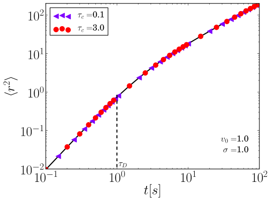
Figure 2: MSD from simulations (colored symbols) for two different correlation times $\tau_{c}$, $\sigma=v_{0}=1.0$, $\Omega=0$, black line corresponds to Eq.(7) with $\alpha=1$, theory and simulation align perfectly, the MSD does not depend on the correlation time $\tau_{c}$ the crossover time from ballistic to diffusive motion is indicated by dashed line at time $\tau_{D}$.

III.2 Distribution of displacements

It is remarkable that the MSD and the diffusion coefficient are independent of the correlation time $\tau_{c}$, so that the underlying correlations cannot be detected from measuring the MSD. Therefore one might expect to observe a Gaussian distribution for the displacements, Eq.(11), for times $t>t_{D}$ and, respectively, the Rayleigh distribution, Eq.(12), for the absolute displacement for all such times. This expectation is however wrong. As we show in the following plots, the probability density of the absolute displacement $P(r,t)$ deviates strongly from the Rayleigh distribution even for times well beyond the crossover time to diffusive behavior $\tau_{D}$. Depending on $\tau_{c}$, the asymptotic convergence to the expected Gaussian and Rayleigh distributions which are independent of $\tau_{c}$ may take place only at times which are considerably larger.

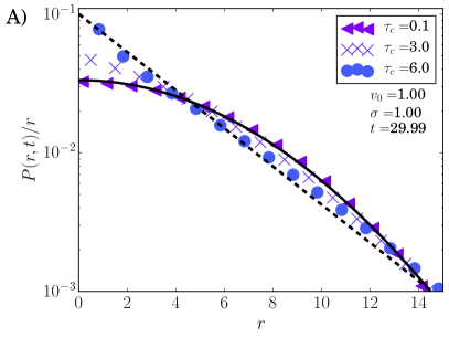
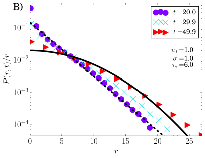
Figure 3: A): log plot of simulation results (colored) for the displacement distributions scaled by $r$ at $t=29.9\gg\tau_{D}$ for given correlation time $\tau_{c}$. Black line corresponds to the absolute displacement distribution Eq.(12) at the given time $t$, with $D_{\text{eff}}$ from Eq.(10),($\alpha=1$). The black dashed line shows the exponential distribution from Eq.(22) with $D_{\text{eff}}$ from Eq.(10), with $\alpha=1$ at the given time.; B): The logarithmic plot of the time evolution displacement distributions rescaled by $r$ for indicated times and parameters. Colored symbols correspond to simulations. The black line corresponds to Eq.(12) for ($t=49.9$). The black dashed line shows the exponential distribution from Eq.(22) with $D_{\text{eff}}$ from Eq.(10),($\alpha=1$) at the given time. At time $t=20.0s$ the displacement distribution (blue circles) displays an exponential behavior and at time $t=49.9s$ (red triangles) it has come closer to a Gaussian.

In Fig. 3A the absolute displacement distributions rescaled by $r$ for three different correlation times $\tau_{c}$ at time $t=29.9$ are shown. The chosen time is well beyond the crossover time $\tau_{D}$ to the diffusion regime, i.e. $t\gg\tau_{D}$, and also much larger than correlation time, $t\gg\tau_{c}$. All three distributions are different. Only for the shortest correlation time the simulation results and the prediction of Eq.(12) (the black line in Fig. 3A) coincide. For longer correlation times the absolute displacement shows an exponential behavior (black dashed line, Eq.(22)). Such behavior is not observed in simulations of particles driven by an OUP with Gaussian white noise. In Fig. 3B the time evolution of the absolute displacement is presented. The results for three different time lags, all within the diffusion regime, are plotted. The black line corresponds to the result of Eq.(12) at time lag t=49.9, with the effective diffusion coefficient according to Eq.(10) with $\alpha=1$. As the simulations show, the distribution (red triangles in Fig.(3B)) at this time has still not fully approached its asymptotic shape (black line). At smaller time lags the displacements clearly deviate from this line, exhibiting an exponential behavior. The black dashed line shows such an exponential decay.

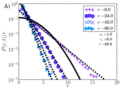
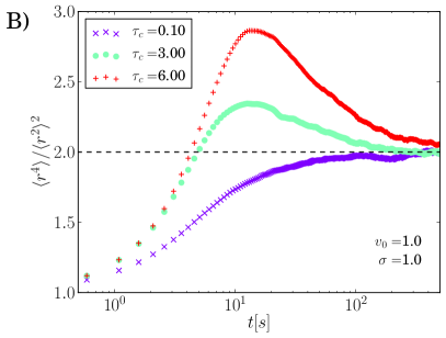
Figure 4: A): Probability densities of displacement distributions scaled by $r$ for various intensities of the Cauchy distributed noise in Eq.(14). Colored symbols correspond to simulations. Black line is the distribution from Eq.(12). Black dashed lines are exponentials from Eq.(22). B): Simulation results for the kurtosis of the distributions for different correlation times. The values approach asymptotically the Gaussian limit (dashed black line) indicating the crossover to a Gaussian displacement distribution.

Fig. 4A shows the the absolute displacement distribution for different values of the noise strength $\sigma$. Colored symbols stand for simulations. The black line shows the Rayleigh distribution from Eq.(12) rescaled by the distance $r(t)$. The black dashed lines are exponentials from Eq.(22)). For higher noise intensities the distributions decay faster. Higher noise intensities correspond to an increase in directional changes which then lead to smaller spatial increments in a given time interval.

It is in principle possible (but tedious) to calculate higher moments of the displacement using Eq.(18). We choose here a phenomenological approach. We make the following exponential ansatz for the normalized distribution density of the displacements with the time dependent characteristic length scale $l(t)$:

$$P(x,y,t|x_{0}=0,y_{0}=0,t_{0}=0)=\frac{1}{2\pi l^{2}(t)}\exp\left(-\frac{\sqrt{x^{2}+y^{2}}}{l(t)}\right)$$ (19)

In agreement with our initial condition, this scale at initial time $l(t_{0})$ should vanish, i.e. $l(t_{0})=0$. For the absolute displacement the probability distribution reads:

$$P(r,t)=\frac{r}{l^{2}(t)}\exp\left(-\frac{r}{l(t)}\right)$$ (20)

We require that the expectation value $\langle r^{2}(t)\rangle$ for the squared absolute displacement (Eq.(20)) is equal to the long time limit of the calculated MSD (Eq.(7))

$$\langle r^{2}(t)\rangle=4D_{\text{eff}}t.$$ (21)

On the other hand, it results from Eq.(20) that $\langle r^{2}(t)\rangle=6l^{2}(t)$. Therefore, the absolute displacement distribution $P(r,t)$ reads:

$$P(r,t)=\frac{3r}{2D_{\text{eff}}t}\exp\left(-\frac{r}{\sqrt{\frac{2}{3}D_{\text{eff}}t}}\right)$$ (22)

The black dashed lines in Fig.(3) and Fig.(4A) correspond to Eq.(22). This distribution fits the simulations very well for times where the displacement is not yet Gaussian, although Eq.(22) does not depend on the correlation time.

Fig. 4B shows simulations for the fourth moment of the displacement divided by the squared MSD (kurtosis). In two dimensions a value of two corresponds to a Gaussian distribution, shown by the horizontal black dashed line in Fig.(4B). A higher value of the kurtosis indicates heavier tails and sharper central peak in the distribution, while a smaller value corresponds to lighter tails and flatter peak. In experiments it can be calculated from the particle positions at different instances of time.

In Fig. 4B the kurtosis for three different correlation times $\tau_{c}$ is plotted. With growing time asymptotically the Gaussian limit is reached for all correlation times. For short correlation times $\tau_{c}\to 0$ the limit is reached from below, while for larger $\tau_{c}$ the kurtosis exhibits a maximum and then approaches the limit from above, indicating the observed transient exponential or heavy-tailed regime. The height of the maximum grows with increasing correlation time, so the deviation from the Gaussian displacement becomes more pronounced in the transient regime. With increasing $\tau_{c}$ the time till the asymptotics is reached also increases.

We give here an estimate of the crossover time $\tau_{G}$ from non-Gaussian to Gaussian displacement distributions. We require, for $t>\tau_{D}$, that the MSD equals the squared correlation length $l_{c}=v_{0}\tau_{c}$, a typical length of the trajectory within the correlation time $t_{c}$ of the noise, i.e.

$$\langle r^{2}(t=\tau_{G})\rangle=l_{c}^{2}.$$ (23)

Note that the length $l_{c}$ differs from the persistence length, as introduced in Eq.(9), being the characteristic scale of transition from ballistic to diffusive motion. Since the particle is already in the diffusive regime the MSD becomes $4D_{\text{eff}}\tau_{G}$ and in consequence we get:

$$\tau_{G}=\frac{v_{0}^{2}\tau_{c}^{2}}{4D_{\text{eff}}}\geq\tau_{D}$$ (24)

For zero torque $\Omega=0$ in Eq.(10) $\alpha=1$ the estimate for the crossover time becomes:

$$\tau_{G}=\frac{\tau_{c}^{2}}{2\tau_{D}}$$ (25)

Comparing this result for $\tau_{G}$ with Fig. 3B indicates that this time $\tau_{G}$ is a lower bound for the establishment of the Rayleigh displacement distribution from Eq.(12). Hence, for $t\gg\tau_{G}$ the distribution of displacements becomes Gaussian.

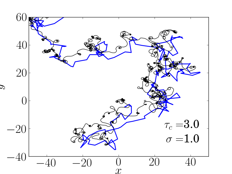
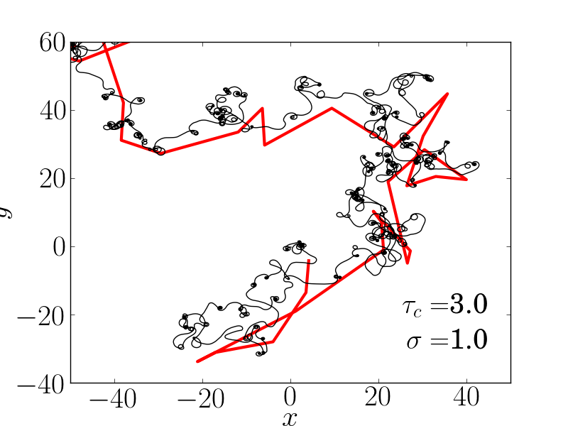
Figure 5: Sample trajectory of OUP driven by Cauchy noise, left: sampling time: $\Delta t=0.05s$ (black) and $\Delta t=5.0s$ (blue), right: $\Delta t=0.05s$ (black) and $\Delta t=40s$ (red), colored trajectories shifted for better visibility

At the end of this section we show a typical trajectory of the process and discuss the importance of sampling time lags. Fig.(5) shows always the same sample trajectory for $\sigma=1$ and $\tau_{c}=3.0$ with different sampling times (black: the sample time lag $\Delta t=0.05s$, blue: $\Delta t=5.0s$, red: $\Delta t=40s$). For the black trajectory positions every $\Delta t=0.05s$ where plotted and connected by a straight line. For the other sampling time lags the same procedure was done accordingly. For the small sampling time lag (black line) one sees a smooth structure with spirals or curls reminding of a run and tumble motion. The curly structure is influenced by the correlation time $\tau_{c}$. Higher correlation time $\tau_{c}$ increases length and size of a spiral. Setting the correlation time close to zero $\tau_{c}\approx 0$ removes the curls and makes the trajectory less smooth (not shown). The blue trajectory in Fig.(5) is the same trajectory as the black one but sampled differently ($\Delta t=5.0s$); the sampling time lag $\Delta t=5.0s$ still belongs to the lags at which non-Gaussian displacement distributions are observed. It still contains some information about the curls. Ignoring the underlying curly structure one might interpret the blue trajectory as one where a particle spends some time in a caged area or is rather immobile (maybe reorients itself) and then moves in rather straight stretches. The red trajectory corresponds to sampling where the Gaussian displacement distribution of displacements during the time lags is established. There are no remnants of the spiral structure visible.

IV Conclusion

We studied the stochastic dynamics of active particles moving at a constant speed whose direction of motion is influenced by an $\alpha$-stable noise source and by a constant torque. First, the noise was considered to be white, later on, we looked at a colored Cauchy noise as generated by an Ornstein-Uhlenbeck process with the characteristic time $\tau_{c}$. The model with white noise generates the motion showing a crossover from the ballistic to the diffusion behavior similar to a behavior for the Gaussian case. The behavior under the colored noise generates the pattern of motion strongly resembling the run and tumble situations or the behavior seen in experiments like Gunther where particles spend some time in confined motion, reorient themselves and then move on. For both physical models we derived analytical expressions for the mean squared displacement and for the effective diffusion coefficient. Astonishingly, in the case of Cauchy-noise, the existence of correlations in the noise does not influence the MSD, the effective diffusion coefficient and the crossover time $\tau_{D}$ from ballistic to diffusive motion coincide for both models with $\alpha=1$. The distribution function of the displacements is however strongly influenced by correlations in the noise even at the times well inside the diffusive regime. In particular, results of numeric simulations for times larger $\tau_{D}$ can be well fitted by an exponential distribution. This exponential behavior appears to be a transient. A crossover to Gaussian distribution of displacements takes place at a third characteristic time $\tau_{G}>\tau_{D}$, connected with $\tau_{c}$ and $\tau_{D}$. This colored noise mechanism might offer an approach to describe observations of a transient non-Gaussian displacement distribution in diffusion experiments like those performed by Wang et al. Wang ; Wangnat . The observed effect is absent in the case of the OUP with Gaussian white noise source, i.e with $\alpha=2$, and becomes the more pronounced, the smaller is the value of $\alpha$.

Generally, our findings underline the importance to investigate the behavior of the higher moments of displacement both in experiments like Seuront ; Bodecker ; Edwards and in simulations. These moments might provide new information on the persistence of the motion. The studied case of the OUP with Cauchy noise is special, and the independence of MSD of the correlation time $\tau_{c}$ of the noise is not a general situation. Nevertheless, we expect deviations from a Gaussian distribution generally in models with a correlated non-Gaussian noise in the angular dynamics, like in Weber_Sok .

V Acknowledgments

This work was developed within the scope of the IRTG 1740 funded by DFG/FAPESP. Lutz Schimansky-Geier acknowledges support from the Humboldt-University at Berlin within the framework of excellence initiative (DFG). The authors thank Dr. B. Dybiec (Krakow) for fruitful discussions.

References

- (1) R. Natan, Proc. Natl. Acad. Sci. 105, 19050 (2008).
- (2) H.U. Bödecker, C. Beta, T.D. Frank, and E. Bodenschatz, EPL 90, 28005 (2010).
- (3) G. Amselem, M. Theves, A. Bae, E. Bodenschatz, and C. Beta, PLOS One 7. e37213 (2012).
- (4) D. Selmeczi, S. Mosler, P. H. Hagedorn, N. B. Larsen, and H. Flyvbjerg, Biophys. J. 89 , 912 (2005).
- (5) B. Rodiek and M.J.B. Hauser, Europ. Phys. Journ.- special Topics, 223, 1199 (2015).
- (6) P. Romanczuk, M. Romensky, D. Scholz, V. Lobaskin, and L. Schimansky-Geier, Europ. Phys. Journ.- special Topics, 223, 1215 (2015).
- (7) M. Romensky, D. Scholz, and V. Lobaskin, J. Royal Soc. Interface 12, 20150015 (2015).
- (8) L. Seuront, A.-C. Duponchel, and C. Chapperon, J. Physica A 385, 573, (2007).
- (9) A. Ordemann, G. Balazsi, and F. Moss, Physica A 325,260 (2003).
- (10) A.M. Edwards, R.A. Phillips, N.W. Watkins, M.P. Freeman, E.J. Murphy, V. Afanasyev, S.V. Buldyrev, M.G.E. da Luz, E.P. Raposo, H.E. Stanley, and G.M. Viswanathan, Nature 449, 1044 (2007).
- (11) J. Gautrais, C. Jost, M. Soria, A. Campo, S. Motsch, R. Fournier, S. Blanco, and G. Theraulaz, J. Math. Biol. 58, 429 (2009).
- (12) S. van Teeffelen and H. Löwen, Phys. Rev. E 78, 020101 (2008).
- (13) S. van Teeffelen, U. Zimmermann, and H. Löwen, Soft Matter 5, 4510 (2009).
- (14) H. Ke, S. Ye, R. Lloyd-Calroll, and K. Showalter, J. Phys. Chem. A 114, 5462 (2010).
- (15) D Takagi, A.B. Braunschweig, J. Zhang, and M.J. Shelley, Phys. Rev. Lett. 110, 038301 (2013).
- (16) B ten Hagen, F. Kummel, D. Takagi, H. Löwen, and C. Bechinger, Nature Communications 5, 4829 (2014).
- (17) K. Pearson, A mathematical theory of random migration, Dulau and Co., London, 1906
- (18) R. Fürth, Zeitschrift für Physik 2, 244 (1920).
- (19) H.C.Berg, Phys. Today, 53, 24 (2000).
- (20) D. Campos, V. Mendez, and I. Llopis, J. Theor. Biol. 267, 526 (2010).
- (21) P. Romanczuk, M. Bär, W. Ebeling, B. Lindner, and L. Schimansky-Geier Eur. Phys. J. Spec. Top. 202, 1 (2012).
- (22) L. Schimansky-Geier, U. Erdmann, and N. Komin, Physica A 351, 51 (2005).
- (23) L. Haeggqwist, L. Schimansky-Geier, I.M. Sokolov, and F. Moss, Eur. Phys. J.– ST 157, 33 (2008).
- (24) F. Thiel, L. Schimansky-Geier, and I.M. Sokolov, Phys. Rev.E 86, 021117 (2012).
- (25) A. S. Mikhailov and D. Meinköhn, Stochastic Dynamics, edited by L. Schimansky-Geier and T. Pöschel (Springer, Berlin, 1997), p. 334.
- (26) W. Blum, W. Riegler, and L. Rolandi, Particle Detection with Drift Chambers, 2nd ed. (Springer, Berlin,2008).
- (27) F. Peruani and L.G. Morelli, Phys. Rev. Lett. 99, 10602 (2007).
- (28) P. Degond and S. Motsch, J. Stat. Phys. 131, 989 (2008).
- (29) C. Weber, P.K. Radtke, L. Schimansky-Geier, and P. Hänggi Phys.Rev.E 84, 011132 (2011).
- (30) C. Weber, I.M. Sokolov, and L. Schimansky-Geier, Phys. Rev. E 85, 052101 (2012).
- (31) P.S. Burada and B. Lindner Phys. Rev.E 85, 032102 (2012).
- (32) W. Ebeling, L. Schimansky-Geier, A. Neiman, and A. Scharnhorst, Fluct. Noise Lett. 5, L185 (2005).
- (33) A. Geiseler, P. H änggi, and G. Schmid, Eur. Phys. J. B 89, 17 (2016).
- (34) A. Godec and R. Metzler J. Phys. A 49, 364001 (2016).
- (35) A. Reynolds, Ecology 89(8), 2347 (2008).
- (36) M.N. Günther, G. Nettesheim, and G.T. Shubeita, Scientific Reports 6, 27972.
- (37) B. Wang, S. M. Anthony, S.C. Bae, and S. Garnick, Proc. Natl. Acad. Sci. USA 106, 15160-15164 (2009).
- (38) B. Wang, J. Kuo, S.C. Bae, and S. Granick, Nature Materials 11, 481 (2012).
- (39) B. Dybiec, E. Gudowska-Nowak, and P. Hänggi, Phys. Rev. E 73, 046104 (2006).
- (40) P.D. Ditlevsen, Phys. Rev.E 60, 172 (1999).
- (41) D. Schertzer, M. Larchevêque, J. Duan, V.V. Yanowsky, and S. Lovejoy, J. Math. Phys. 42, 200 (2001).
- (42) B. J. West and V. Seshadri, Physica A 113, 203 (1982).
- (43) P. Garbaczewski and R. Olkiewicz, J. Math. Phys. 41, 6843 (2000).
- (44) G.E. Uhlenbeck and L.S. Ornstein, Phys. Rev. 36, 823 (1930).