Proteins analysed as virtual knots

Abstract

Long, flexible physical filaments are naturally tangled and knotted, from macroscopic string down to long-chain molecules. The existence of knotting in a filament naturally affects its configuration and properties, and may be very stable or disappear rapidly under manipulation and interaction. Knotting has been previously identified in protein backbone chains, for which these mechanical constraints are of fundamental importance to their molecular functionality, despite their being open curves in which the knots are not mathematically well defined; knotting can only be identified by closing the termini of the chain somehow. We introduce a new method for resolving knotting in open curves using virtual knots, a wider class of topological objects that do not require a classical closure and so naturally capture the topological ambiguity inherent in open curves. We describe the results of analysing proteins in the Protein Data Bank by this new scheme, recovering and extending previous knotting results, and identifying topological interest in some new cases. The statistics of virtual knots in protein chains are compared with those of open random walks and Hamiltonian subchains on cubic lattices, identifying a regime of open curves in which the virtual knotting description is likely to be important.

Introduction

Proteins are large, complex biomolecules exhibiting folded conformations, whose precise form and stability are fundamental to their biological role branden98 . As protein chains can be thought of as long, tangled curves, it is natural to ask if they can be knotted. Mathematical knot theory only defines knots in closed, circular loops adams94 , whereas the curves described by protein chain backbones have distinct endpoints. They are open chains formed from a string of carbon and nitrogen atoms and may be ‘untied’ by smooth deformation. A degree of mathematical compromise is therefore required to determine whether a given protein chain may be considered knotted millett13 ; tubiana11 ; its termini must somehow be joined to make a closed curve, without distorting the protein’s configuration. Various closure constructions have been proposed tubiana11 , generally giving similar results, and applied to protein chain catalogues pdb ; knotprot . These investigations have shown that knotting in proteins is in fact very rare knotprot ; lua06 , likely owing to the chemical and mechanical difficulty of forming such structures making them evolutionarily disadvantageous mallamjackson12 . The unlikelihood of knotting might suggest an evolutionary advantage when they do occur faisca15 ; lim2015 , but it remains unclear in most cases exactly how this manifests mallamjackson12 ; lim2015 .

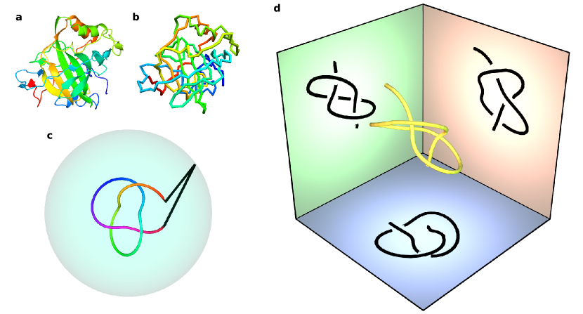
Figure 1: Protein backbone structures as open knotted space curves. (a) shows the backbone and some secondary structure of the protein with PDB ID 4COQ, chain A (Thermovibrio ammonificans alpha-carbonic anhydrase) 4COQAjames14 , while (b) shows only the backbone chain of carbon alpha atoms as a piecewise-linear space curve. The colouring along the chain serves only to distinguish different regions and does not have physical meaning. (c) represents the closure of an open curve by straight lines from its termini to a point on a surrounding sphere. (d) shows a 3-dimensional open curve and its planar projections in three perpendicular directions; each projection here gives an open knot diagram, where each crossing in the projection indicates which strand passes over or under the other. In this example, each of these projected knot diagrams represents one of two different knot types, as explained in the text.

Fig. 1(a) shows a ribbon diagram representation of a protein chain. Secondary structures (shown as alpha helices and beta pleated sheets), as well as bonds other than peptide bonds such as disulphide bonds and hydrogen bonds, will be ignored in the following analysis, despite some recent investigation of their conformational tangling haglund14 ; dabrowski-tumanski16 ; flapan15 ; cao05 ; boutz07 ; mcdonald93 . The corresponding protein backbone is shown in Fig. 1(b) as a piecewise-linear curve, with each vertex representing a carbon alpha atom, each connected to its two neighbours, or one neighbour at the termini. The most obvious way of closing the backbone into a closed loop is to join its endpoints with a straight line, but such a crude procedure usually fails to give a knot representative of the protein tubiana11 ; millett13 . A method that has become standard millett13 ; knotprot ; lua06 is illustrated in Fig. 1(c): straight lines are continued from each backbone terminus to the same point on a sphere surrounding the curve (we refer to this as sphere closure). Each point on the closure sphere gives a closed curve of specific knot type, which may be the ‘unknot’, equivalent to the trivial circle. Nongeneric closures where the straight lines intersect the backbone are ignored. The sphere is given a large enough radius to avoid small-scale geometrical effects; in practice, the closing lines can be taken as parallel, closing ‘at infinity’ (i.e. the sphere has infinite radius). Labelling each point on the sphere by the knot resulting from closure there partitions the sphere surface into ‘islands’ of different knot types, and the island covering the greatest area may be identified as the ‘knot type’ of the protein. The results of the ongoing KnotProt protein survey knotprot (as of Sep 2016) reveal that according to this definition, 946 of the 159,518 sequence unique protein chains in the Protein Data Bank pdb (PDB) are statistically knotted by this measure.

Here we present an alternative analysis of protein knots. Rather than closing the backbone curve in 3D, we consider the projection of the open curve in every direction. Each such projection gives a 2-dimensional open knot diagram, a network of arcs intersecting at crossing points, where one arc passes over the other adams94 . Examples are represented for three perpendicular projections of a simple open curve in Fig. 1(d). The topological analysis is performed on the knot diagrams by considering them as virtual knots via a virtual closure that does not add additional classical crossings. Virtual knots are a generalisation of the usual ‘classical’ knots, that can capture the open nature of the diagram via new virtual knot types that do not correspond to a closed classical knot (although classical knots may also result from this procedure) kauffman99 .

The topological character of the open protein backbone chain is fully characterised by the distribution, over different projection directions, of different classical and virtual knots resulting from virtual closure. An advantage of this new method is that it allows a more subtle refinement of the knot distribution associated with an open curve, as the inclusion of virtual knots can better capture the conformations of backbones where tangling is evident but no single knot type dominates. This analysis is particularly suitable for protein curves, and relates to the distinction between deep knots (whose knotting is strongly classical) and shallow knots (whose topological spectrum becomes significantly richer under virtual knotting). We quantify these changes, and suggest how these techniques could apply to specific other systems of open curves.

Methodology and Results

Projected open curves and virtual knots

In this Section we summarise some basic mathematics of knot and virtual knot classification adams94 ; kauffman99 . A more complete summary of both classical and virtual knot theory is given in Supplementary Note 1.

Knots are labelled and ordered in knot tables rolfsen76 ; hoste98 ; knotatlas ; knotinfo according to their minimal crossing number $n$, which is the minimum number of crossings a 2-dimensional diagram of the knot may have adams94 . The closed knots are labelled $n_{m}$, where $m$ counts the knots of minimal crossing number $n$, not distinguishing enantiomeric pairs with opposite chirality (indeed, we do not distinguish between such pairs here, although it would be possible to do so). Examples of some simple knots appear in Fig. 2(a), such as the trefoil knot $3_{1}$ (the only knot with $n=3$) and the only two five-crossing knots $5_{1}$, $5_{2}$. Composite knots, in which more than one knot is tied in a single curve, do not appear in protein chains knotprot . A given knot has many possible conformations, which may have arbitrarily many crossings in projection; equivalent conformations (which can be deformed into one another without cutting and joining) are said to be ambient isotopic, and their diagrams can be related by a sequence of Reidemeister moves adams94 (see Supplementary Fig. 1).

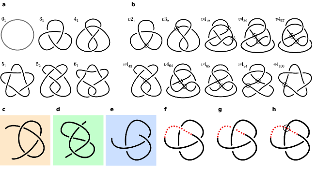
Figure 2: Classical and virtual knot diagrams which could occur as closures of open curves. (a) shows the first six classical knots in the standard tabulation (including the unknot $0_{1}$); all but $5_{1}$ have been identified as dominant knot types in at least one protein knotprot . (b) shows the virtual knots with $n=2,3,4$ as tabulated in virtualknottable , all of which can arise as virtual closures of open knot diagrams. Virtual crossings are shown as circles. (c)-(h) show examples of open diagrams, which may be identified under virtual closure as classical or virtual knots. (c)-(e) are equivalent to the projections from Fig. 1(d). (f) and (g) show (e) closed with a classical arc passing above or below the intervening strands, forming an unknot $0_{1}$ and trefoil knot $3_{1}$ respectively, while (h) shows (e) closed instead with a virtual crossing to produce the knot $v2_{1}$.

Open curves are technically not knots, as they do not form a closed loop and so have endpoints. We instead close the endpoints with an arc that makes virtual crossings with the other arcs, which do not distinguish over or under crossing. Under this virtual closure each open diagram represents a virtual knot kauffman99 , a generalisation of normal knot diagrams. All the topological information is contained within the classical crossings (in this sense, the virtual crossings represent ‘not closing’ the curve), so the virtual crossings capture the ambiguities between the different classical closures. A given open knot diagram has the same virtual knot type under all possible virtual closures, although this may still represent a classical knot (and all classical knots can arise from virtual closure). This procedure is illustrated in Fig. 2(c)-(e): in (c) and (d) the endpoints can be closed with no additional virtual crossings, in both cases representing the classical trefoil knot $3_{1}$, while in (e) there is no way to avoid crossing an intervening strand. Fig. 2(f) and (g) show the ambiguity of classical closure, resulting in the unknot $0_{1}$ and trefoil knot $3_{1}$ respectively, while in (h) the virtual closure produces a single virtual knot. We note that open knot diagrams could instead be considered in the slightly wider class of classical knotoids turaev12 , whose isotopies are determined by augmented Reidemeister moves which forbid endpoints from passing over/under any strand of the curve, but although knotoids form their own topological classes turaev12 ; gugumcu16 they have not yet been robustly tabulated (see Supplementary Note 1). Our method corresponds to the virtual closure of the classical knotoid gugumcu16 .

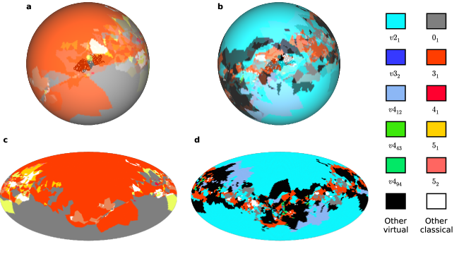
Figure 3: Classical and virtual knot types found amongst different projection/closure directions for a protein backbone chain. The protein backbone shown has PDB ID: 4K0B, chain A (Sulfolobus solfataricus S-adenosylmethionine synthetase) 4K0BAwang2014 . The points of each sphere are coloured according to the knot type (classical or virtual) found by closure/projection in that direction. (a) shows the classical knots resulting from sphere closure at each point, with knot types according to the legend, while (c) shows the same colouring in an area-preserving (Mollweide) projection of the sphere, making its entire area visible. (b) shows the virtual knot types resulting from projection in each direction on the sphere, and (d) the same colouring again by projection. These images are constructed from sampling $10,000$ directions in each case. Antipodal points on the sphere are always associated with the same knot type under virtual closure (up to possibly distinct mirrors for certain virtual knot types), but may produce different classical knots on sphere closure.

Tabulations of virtual knots virtualknottable ; kauffman99 follow the same ordering logic. We denote virtual knots with a prefix ‘$v$’, i.e. $vn_{m}$ where $n$ is again the minimum classical crossing number (there is no relationship between the classical $n_{m}$ and virtual $vn_{m}$), with examples given in Fig. 2(b). $n$ is invariant to (appropriately generalised) ambient isotopy and ‘virtual’ Reidemeister moves (see Supplementary Note 1). As with the classical tabulation, all mirror-symmetric partners are considered to be equivalent. Not all virtual knots can arise from virtual closure of open diagrams. The only ones that can occur are those that can be drawn with all virtual crossings adjacent, with no classical crossings in between (i.e. along the closure arc); the examples with up to 4 classical crossings are shown in Fig. 2(b). There are still many more of these than classical knots for given $n$: the classical (virtual) count is 1 (0) for $n=0$; 0 (1) for $n=2$; 1 (1) for $n=3$; 1 (8) for $n=4$, etc.

In practice, the knot type (classical or virtual) of each closed diagram is found through calculation of knot invariants adams94 ; rolfsen76 ; kauffman99 ; virtualknottable , which are functions of the diagram whose values depend only on its (classical or virtual) knot type. Most readily-calculated invariants fail to distinguish certain distinct knots adams94 , so we identify types by the characteristic signatures of a set of invariants, calculated sequentially until the knot type is clear (after additionally simplifying each diagram algorithmically using Reidemeister moves). It is more computationally efficient to calculate polynomial invariants at specific values rather than symbolically, and we consider them at certain roots of unity taylor16 . For classical knots, invariants are: the Alexander polynomial adams94 $\Delta(t)$ at $t=-1$ (the knot determinant adams94 ), $t=e^{2\pi i/3}$ and $t=-i$. For virtual knots we use the generalised Alexander polynomial kauffman03 ; virtualknottable $\Delta_{g}(s,t)$ at $(s,t)=(-1,e^{2\pi i/3})$, $(-1,i)$, $(e^{2\pi i/3},i)$; and the Jones polynomial $V(q)$ jones85 ; adams94 ; rolfsen76 ; kauffman1987 at $q=-1$. Classical knots have $\Delta_{g}=0$.

We will present results on knotting in terms of the fractions of directions giving different knot types under sphere or virtual closure. Fig. 3(a)-(b) demonstrate this structure for an example protein chain, by colouring the sphere according to the knot types found in each direction from both of the closure methods, while (c) and (d) show the same results in an (area-preserving) Mollweide projection of the sphere area such that its entire surface is visible; this projection is preferred in later figures. In the sphere closure map (c), many of points are unknotted (grey), yet 59% give a trefoil knot $3_{1}$, which therefore dominates and so this backbone was determined by knotprot to be $3_{1}$ knotted. The smaller islands where closures form more complex knots make up less than 7% of the sphere area. In the corresponding virtual closure map (d), the virtual knot $v2_{1}$ is associated with much of the area identified as $0_{1}$ or $3_{1}$ in (c), now appearing in 54% of different projections. This curve therefore has strong virtual character, and its virtual knot type reflects the ambiguity of the open curve between the unknot and trefoil knot.

Analysis of the Protein Data Bank

We now present the results of our survey of knotting in the Protein Data Bank (PDB) pdb , using both sphere closure and virtual closure. Following the methodology of the KnotProt database knotprot , we constructed a minimal set of distinct chains from the 121,532 structures recorded in the PDB, analysing only each sequence unique chain in a given protein and rejecting chains containing artefacts. We additionally restrict attention to chains that have not been made obsolete by more recent measurements. The PDB records for some of the remaining proteins have broken chains (where the chain conformation is uncertain), which we close with straight lines. This gives a total of 159,518 protein chains for analysis. For each chain, we close/project to 100 different points on the sphere (approximately uniformly distributed following the method of rakhmanov94 ), considered sufficient for reasonable numerical confidence at acceptable computational cost millett13 .

The sphere closure analysis of KnotProt found 946 knotted chains, including 871 trefoil ($3_{1}$) knots, 45 occurrences of $4_{1}$, 27 of $5_{2}$ and 3 of $6_{1}$ (at time of comparison: Sep 16). Our corresponding analysis gives instead $972$ knotted chains, including 894 of $3_{1}$, 48 of $4_{1}$, 27 of $5_{2}$ and 3 of $6_{1}$, but does include all but one of the KnotProt-identified chains, leaving 27 additional knot detections. These discrepancies appear to arise from small differences in methodology, particularly in rare occasions where very severe chain breaks are present; 17 of our extra detections are considered knotted by one or both of the alternative protein knots databases pKNOT lai07 , or Protein Knots kolesov07 . We therefore consider that our sphere closure methodology accurately detects protein knotting for the purpose of comparison with virtual closure.

In the above results, the knot associated with an open chain is the most common single knot type occurring over sphere closure in different directions (i.e. the modal average). Although this methodology is natural, this can miss certain interesting cases; for instance, a chain closing in different directions to 40% unknot, 30% $3_{1}$ and 30% $4_{1}$ would be considered unknotted, despite giving some knot for the majority of closure directions. Such cases are much more frequent under virtual closure, as many more knot types are possible, and the resulting maps are correspondingly more complex as shown in Fig. 3. We therefore introduce new classes of knotting associated with open chains, based on the definition that an open chain is unknotted only if it appears to be $0_{1}$ in over 50% of closure directions; it is otherwise considered knotted, in some sense. For sphere closure, if a single (nontrivial) knot type occurs in at least 50% of directions we call this strongly knotted, while if the sum of different nontrivial knot types occurs for at least 50% of directions, but no single type does, we call this weakly knotted. This does not significantly affect the 972 protein knots discussed above; almost all (968) are strongly knotted by these definitions, with 7 further chains being weakly knotted. The choice of threshold at 50% is somewhat arbitrary, and the number of curves identified as unknotted rises (falls) as it is increased (decreased).

empty

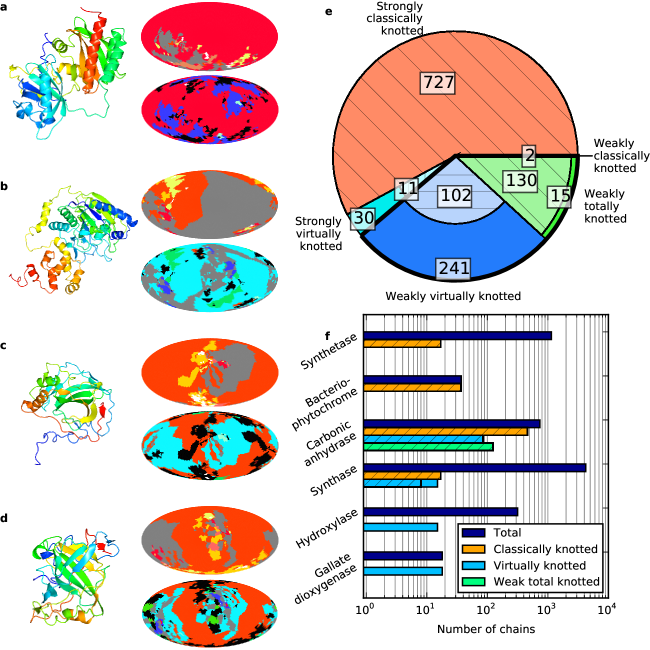
Figure 4: Results of virtual closure analysis for knotting in the Protein Data Bank. Knot categorisations follow the main text; strong classical (virtual) knotting where more than 50% of projections form the same classical (virtual) knot type; weak classical (virtual) knotting when over 50% of projections form classical (virtual) knots but no single knot type dominates, and weak total knotting where the unknotting fraction does not exceed 50% but no other specific class dominates. (a)-(d) give examples of knot type maps (see Fig. 2) for protein chains in these different classes, with colours following the legend of Fig. 3. The upper map in each case shows the results of sphere closure, while the lower shows virtual closure: in (a) PDB ID: 4E04, chain A (Rhodopseudomonas palustris RpBphP2 chromophore-binding domain) 4E04Abellini2012 , which is classically knotted in both cases, although the virtual closure reveals new structure; in (b) PDB ID: 3WKU, chain B (sphinogobium sp. SYK-6 extradiol dioxygenase)  3WKUBsugimoto2014 , which is not knotted under sphere closure but is strongly virtually knotted under virtual closure; in (c) PDB ID: 4XIX, chain A (Chlamydomonas reinhardtii carbonic anhydrase) 4UELAel2010 , which is knotted under both sphere and virtual closure, weakly virtually knotted in the latter; and in (d) PDB ID: 3KIG, chain A (Homo sapiens carbonic anhydrase II mutant) 3KIGwischeler2011 , which is knotted under sphere closure and exhibits weak total knotting on virtual closure. (e) summarises the number of protein chains in each knotting class under virtual closure. (f) shows knot types found amongst selected categories of protein chain names, and their distribution amongst knotting classes. In both (e) and (f), hatched areas represent chains which were also identified as knotted under sphere closure.

Under virtual closure, the different projections may include a mixture of virtual and classical knot types. We refine the distinction of strong and weak knotting to distinguish some major categories of knot character, calling a chain strongly classically (virtually) knotted where a single classical or virtual knot type appears in more than 50% of virtual closures from different projection directions (e.g. strongly trefoil knotted or strongly $v3_{2}$ knotted). A chain is instead weakly classically (virtually) knotted if no knot type is so individually common, but a combination of different classical (virtual) knot types alone contributes to over 50% of projection directions (e.g. 30% $v3_{1}$, 30% $v2_{1}$ and 40% $0_{1}$ is weakly virtually knotted). In all other cases, no specific classification dominates, and we call the curve weakly totally knotted. All of these weak classes represent knots with significant topological character that is not consolidated in forming a single deep knot. Examples of protein chains according to these classifications are shown in Fig. 4(a)-(d), and the identifications may vary significantly from the results obtained by sphere closure: (a) is strongly classically knotted according to both analyses; (b) was unknotted on sphere closure but is strongly virtually ($v2_{1}$) knotted on virtual closure; (c) was strongly $3_{1}$ knotted on sphere closure but is weakly virtually knotted on virtual closure; and (d) was strongly $3_{1}$ knotted on sphere closure but on virtual closure is weakly totally knotted.

Altogether we find 1258 protein chains falling into one of these topological classes, 283 more than in our sphere closure analysis. The mix of their different classifications is summarised in Fig. 4(e). As with the sphere closure analysis, most of these protein chains are strongly classically knotted (727 cases, all of which were also strongly classically knotted under sphere closure, and mostly the knot $3_{1}$), and weak classical knotting is still negligible (2 cases, 7 under sphere closure). Strong virtual knotting is much less common, occurring in 41 cases, 30 previously considered unknotted under sphere closure. These are cases where two classical knot types compete with comparable area contribution under sphere closure, and in all but one case the competition is between $0_{1}$ and $3_{1}$; the virtual knots are therefore strongly $v2_{1}$ knotted (the remaining example is $v4_{43}$ between classical types $0_{1}$ and $5_{2}$).

The remaining protein chains are weakly knotted in some form; 343 are weakly virtually knotted (around a third of which were not topologically interesting under sphere closure), and 145 are weakly totally knotted (most of which were dominated by a classical knot under sphere closure). The new detections here represent curves that cannot be easily identified with a single classical knot type because their conformations are similar to multiple classical knots. This is demonstrated in Fig. 4(c), whose knot types under sphere closure suggest little of the complexity evident in its virtual closure map; this feature is typical of the weak virtual knots, which for this reason include most of the new chains that appeared unknotted under sphere closure. These knots may be interpreted as being rather shallow, as small modifications to the chain can relatively significantly affect the maps. The weakly totally knotted chains are similar but with the classical knots a little deeper in the chain, as in the example of Fig. 4(d), where the clarity of the chain’s trefoil knot character is muted but not removed under virtual closure.

These various classifications of strong and weak knots form a loose way of capturing the forms of knotting and tangling exhibited in protein backbone curves, with physical implications for the depth of the knots in the chain. The distribution of these classes is uneven amongst the protein chains; for instance, all 46 examples of $4_{1}$ under sphere closure remain strongly $4_{1}$ knotted under virtual closure, suggesting consistently small virtual character. Knotting is also not equidistributed amongst different protein classes: Fig. 4(f) shows a breakdown of the the different classes of knotted open chain by protein chain name, for families in which knotting has previously been observed to cluster knotprot , as well as families where new virtual character appears. Virtual knotting appears significant amongst carbonic anhydrases, in which the knots are known to be rather shallow, and all knots found under virtual closure also appear under sphere closure. In contrast, the virtual knots amongst synthases are almost all newly identified, with previously discovered strong classical knots being deep enough to remain unchanged by the analysis. Further, the families of hydroxylases and gallate dioygenases contain several examples of virtual knotting, and neither family showed any evidence of knotting under sphere closure. It is unsurprising that the levels of topological complexity are consistent among members of the same protein families, as they arise from consistent features in their secondary and tertiary structures, but it is important that virtual knotting has its own distribution among protein chain names, distinct from that of classical knotting.

Comparison with random open chain ensembles

The virtual closure technique for describing knotting is applicable to any open space curve, but the the presence of virtual knots relies on particular geometric characteristics of the curve. It is unclear if proteins express these in a generic fashion, or if virtual knotting is a particularly good (or bad) descriptor of their backbone chains, and for comparison we perform a preliminary analysis by sphere closure and virtual closure for other families of random open curves. These are drawn from two statistical ensembles: open random walks, and open subchains of Hamiltonian walks on a cubic lattice. In order to investigate the new information provided by virtual knotting we use a simplification of the scheme in the previous section, considering an open curve as ‘knotted’ if over 50% of directions yield a knot on sphere closure (i.e. either strong or weak classical knotting), and ‘virtually knotted’ if over 50% of projection directions are virtually knotted (i.e. either strong or weak virtual knotting). Virtual closure is a useful technique for ensembles where the virtual knotting probabilities are comparable to or higher than closure knotting probabilities, otherwise most curves will take the same strong knot type under both analyses. The main parameter against which knotting is compared is closing distance fraction (CDF)—the distance between the curve’s endpoints divided by its total length—which varies from 0 for a closed loop, to 1 for a straight line.

Random walks consist of a sequence of random linear steps, whose limiting, long-length statistical behaviour is that of Brownian motion. Their geometry and topology is quite well understood; for sufficiently long walks, the statistics are independent of the specific model, tending towards the characteristic Brownian fractal behaviour falconer97 . The probability of knotting in closed random walks has been well investigated orlandini07 . Random walks tend not to be a good model for proteins, but nevertheless are good models for other physical systems flory53 ; orlandini07 ; taylor16 , and are a convenient comparison model for knotting of open chains in the absence of physical constraints.

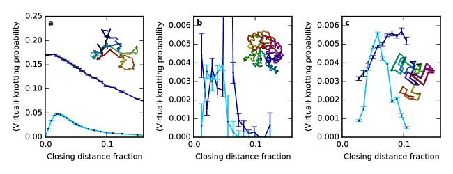
Figure 5: Knotting and virtual knotting probabilities in different open curve ensembles. The closing distance fraction (CDF) is the ratio of the distance between the open curve’s endpoints with respect to the total curve length. Knotting probabilities are given (a) $6\times 10^{6}$ open random walks of length 100; (b) all 159,518 proteins analysed in the previous Section, with various lengths and binned according to CDF; (c) $5.5\times 10^{6}$ length-75 subchains of Hamiltonian walks on cubic lattices of side length 6, binned by CDF. In (c), the large fluctuations reflect correlations implicit in the lattice. In each figure, the inset shows a typical example of the curve ensemble, coloured red to blue by hue along its length to distinguish different regions of the curve. Error bars represent the standard error on the mean probability of the knot statistic.

Fig. 5(a) shows the statistics of knotting upon sphere and virtual closure for a set of random walks with 100 steps generated via the method of cantarella12 , with inset showing a sample random walk. The advantage of this particular ensemble is that the CDF can be directly controlled, but for all distances knotting is significantly more common than virtual knotting (this is most probable around a CDF of 0.025, where about 5% of the random walks are virtually knotted, but even at this value classical knotting is at least 3.5 times as common). This qualitative result appears to hold for random walks of very different lengths (not shown). These results are not surprising as knots in random walks can easily be small, localised deep within the chain.

This contrasts strongly with the equivalent results for proteins, shown in Fig. 5(b), which combine all protein chains from the previous Section despite their backbones being of many different lengths (from tens to thousands of angstroms and up to $\sim$3300 carbon atoms in the backbone chain). The comparatively small number of protein chains mean the statistics are only useful for qualitative comparison. Nevertheless, virtual knotting appears far more likely relative to classical knotting, possibly becoming more dominant around a CDF of 0.025.

Unlike random walks, protein backbones are characterised by relatively compact geometries (such as the inset to Fig. 5(b)), and aspects of this this can be reproduced by simple mathematical models of random chains. In Fig. 5(c), we give the results for one such model: a subchain of a Hamiltonian walk lua06 , that is, a path on a cubic lattice of fixed size, visiting every vertex once and every edge no more than once. Such curves form a confined, folded structure due to the strict boundaries of the finite lattice. The geometry and topology of proteins are best approximated when the Hamiltonian segment is much shorter than this, such that the lattice confinement is not strong, and random lattice walks of this type can be efficiently generated up to lattice side lengths of at least 10 lua04 .

Fig. 5(c) shows the knotting and virtual knotting sampled from $5.5\times 10^{6}$ random Hamiltonian subchains with length 75 on a cubic lattice of side length 6, with these parameters chosen to approximate the knotting probabilities in Fig. 5(b). Here the virtual knotting is strong relative to closure knotting, comparable to proteins but very unlike random walks, and the probability of virtual knotting exceeds that of classical knotting across the small range $0.04\lesssim$ CDF $\lesssim 0.055$. This trend appears to be highly robust to different parameters; even if the lattice is saturated, such that knots are very common, virtual knotting exceeds classical knotting over approximately the same range. These results emphasise that virtual knotting is a generic feature of certain geometrical classes of curves, arising from relatively weak geometric constraints even in the absence of the physical complexity of protein chains.

Discussion

We have shown that the backbones of protein chains, as well as other open curves, can be described topologically in terms of virtual knotting. Through the method of virtual closure of projections, open chains are found to have a much wider set of topological classes than the classical knots in closed curves, and we have found many examples of different virtual knot types, in projections of protein chains. Nevertheless, virtual knotting dominates relatively few proteins, and the virtual knot types which do occur are only a small fraction of the possible virtual knots. In some cases this can be thought of as representing a more nuanced characterisation of ‘almost’ knotted curves, softening the binary distinction between knotting and unknotting imposed by traditional closure methods. In the analysis of proteins the most dominant virtual class is the weak virtual knots, where no single knot type is most prevalent but less than 50% of projected diagram directions are unknotted. These curves are the most topologically ambiguous, and cannot be associated with a definite knot type.

Protein chains express several geometrical properties that might be expected to encourage virtual knotting: as they fold they curve and twist into relatively small, chemically bound structures such that their projections have many crossings; the endpoints of the protein backbone are often within or near the surface of the structure, such that projections in different directions produce distinctly different knot diagrams; and the physical limits on their curvature and overall tangling mean that knots are rarely unambiguous local structures but inherently involve the entire protein chain. This is not true for random walks, and indeed virtual knotting was found to be less significant in them, although Hamiltonian subchains, which do have some of these properties, were found to be particularly strongly virtually knotted. We expect that virtual knotting analysis will be most relevant in other systems of open curves with compact configurations. A mechanism that might encourage virtual knots in physical systems is tight confinement, such as that of a curve confined within a sphere (e.g. DNA within a viral capsid marenduzzo2013topological ; diao14 ) but also between less confining barriers such as adjacent planes orlandini13 ; micheletti12 , which might privilege certain projection directions.

Under the virtual closure analysis, a single chain can project to many different classical and virtual knot types, which we have summarised by emphasising ‘strong’ dominating single knot types, or the ‘weak’ classes of mixed classical and virtual knot types. Although this captures some differences in the tangling of open curves, it ignores the rich structure of knot types in the projected map, other details of which may be necessary to understanding the 3D spatial conformation of the open chain. Including virtual knots may be important to understand these maps, not only because the number of possible types is increased, but also because they generally occur in between classical knot types (seen clearly in Figs 3 and 4(b)-(d)), even in chains which are mostly unknotted. This extra discriminatory ability would be useful in any classification of open curve geometry according to these deeper projection correlations, and could also apply to any investigation of topological character over time in dynamic systems, capturing the intermediate stages between unknotting and unambiguous classical knotting.

Although we have focused our discussion on the statistics of virtual knotting in protein backbone chains, the analysis only requires that the curves are open-ended; virtual closure is a refinement rather than an alternative to existing methods of analysing knotting in open curves, and can be applied anywhere in place of sphere closure of the open chain. This could include other aspects of protein knotting, such as slipknotting in which knots appear in subsections of the curve before disappearing as the rest of the curve ‘unthreads’ itself sulkowska12 . Many examples of slipknotting have been found in proteins knotprot , and tracking the knot type across subchains of the full protein backbone produces a slipknotting fingerprint. Extending these methods to include virtual knots via virtual closure would be natural, as virtual knots would typically occur at transitions between different classical knot types. The methodology also can be further extended, for example to systems of multiple open curves under similar average closures which extend in the same fashion to the theory of virtual links (and potentially to a wider class of virtual knot types), and may even extend to other knot-like objects such as protein lassos dabrowski-tumanski16 .

Methods

Knot detection by sphere closure of open curves. For each open chain (here, a protein backbone or random walk), each direction (point on a sphere around the curve) is associated with a type of knot. For the sphere closure analysis, the endpoints of the open curve are closed by extending them ‘to infinity’ in this direction, giving a closed curve of a specific classical knot type. In practice, the 3D chain is projected in the plane perpendicular to this direction, then the diagram closed with a straight line that passes over every intervening arc of the diagram. Each open curve is projected and analysed in 100 approximately uniformly distributed closure directions, chosen using the algorithm of rakhmanov94 . Previous work has verified that 100 closure directions is usually sufficient to determine the significant statistical behaviour of closures in different directions millett13 , and so alternative approximately-uniform samplings should reproduce the same statistics. For each projection, the resulting knot diagram is algorithmically simplified using Reidemeister moves (see Supplementary Note 1), then the knot type identified through the calculation of knot invariants as described in the main text. The invariant used is the modulus of the Alexander polynomial, $|\Delta(t)|$, evaluated at each of $t=-1$, $t=e^{2\pi i/3}$ and $t=i$, computed using a standard scheme orlandini07 . The Alexander polnomial is used because it can be calculated in polynomial time in the number of crossings of a knot diagram (more discriminatory invariants are harder to calculate), but it is still sufficient to distinguish unambiguously knots with up to at least 8 crossings; more complex knots may have invariants taking the same values, but these complex conformations are rare and never dominate in protein chains (for instance, the next knot with the same Alexander polynomial as the trefoil knot $3_{1}$ has 13 crossings, and no simpler knot agrees at the roots of unity we consider either). For simple knots this choice of three evaluation values is just as discriminatory as the full Alexander polynomial, but more convenient for numerical calculation.

Knot detection by virtual closure of open curves. For the virtual closure analysis of open curves, the selection of projection directions proceeds according to the above method, but the projected diagram in a given direction is closed instead with virtual crossings and simplified algorithmically using both classical and virtual Reidemeister moves (see Supplementary Note 1). The same 100 projection directions are used (and 100 directions appear sufficient to distinguish knot types as in the sphere closure analysis). Virtual knots require different invariants, we use the generalised Alexander polynomial $\Delta_{g}(s,t)$ at certain pairs of arguments ($s=-1$, $t=e^{2\pi i/3})$), ($s=-1$, $t=i$) and ($s=e^{2\pi i/3}$, $t=i$). Unlike the classical knots, even the simple virtual knots $v2_{1}$, $v3_{1}$ and $v4_{94}$ have equal $\Delta_{g}(s,t)=(-s^{-2}+s^{-1})t^{2}+(s^{-2}-1)t^{-1}+(-s^{-1}+1)$. In these cases we additionally calculate the Jones polynomial $V(q)$ at $q=-1$ adams94 , which requires exponential time in the crossing number but unambiguously distinguishes all these examples. Some more complex virtual knots would also be ambiguous to these measurements but, as with the classical knots in sphere closure, are far more complex than those appearing in protein chain closures. Some virtually closed diagrams represent classical knots, in which case $\Delta_{g}(s,t)=0$ and the Alexander polynomial is used as above. These cases are still occasionally complex virtual knots with vanishing $\Delta_{g}$, so we further calculate whether the classical knots produced from over- and under- closure of the virtual crossing arc are the same; although not proven, we anticipate that if their knot types differ the diagram likely represents a virtual knot, whose type we do not identify. In practice, such cases make up a negligible fraction of total projections and do not limit the analysis.

Numerical analysis of protein backbone chains. The protein chains are obtained from the list of all recorded protein molecules in the Worldwide Protein Data Bank (PDB) berman03 . In each case the .pdb protein record is downloaded and parsed using ProDy prody . In particular, we parse the atomic coordinates of each carbon alpha atom, and reconstruct the protein backbone by connecting these sequentially with straight lines. This is an approximation to the true NCCNCC backbone. In some cases there are missing residues in the PDB record, and here the distant carbon alphas across any breaks are connected with straight lines to create one, continuous open curve for each protein chain. We also ignore heteroatom structures. Where protein chain names are referenced in the text, these are as recorded in the PDB. Protein ribbon structure images were created using CCP4mg mcnicholas2011 .

Acknowledgments

The authors are grateful to Ben Bode, Paula Booth, Neslihan Gügümcü, Lou Kauffman, Annela Seddon, Joanna Sulkowska and Stu Whittington for valuable discussions. This research was funded by the Leverhulme Trust Research Programme Grant No. RP2013-K-009, SPOCK: Scientific Properties of Complex Knots. Keith Alexander was funded by the Engineering and Physical Sciences Research Council. This work was carried out using the computational facilities of the Advanced Computing Research Centre, University of Bristol.

Author contributions

KA carried out the protein analysis and virtual knotting routines. AJT carried out the classical knot identification and random chain analysis, and suggested the original problem. MRD directed the study and drafted the manuscript.

Competing financial interests

The authors declare no competing financial interests.

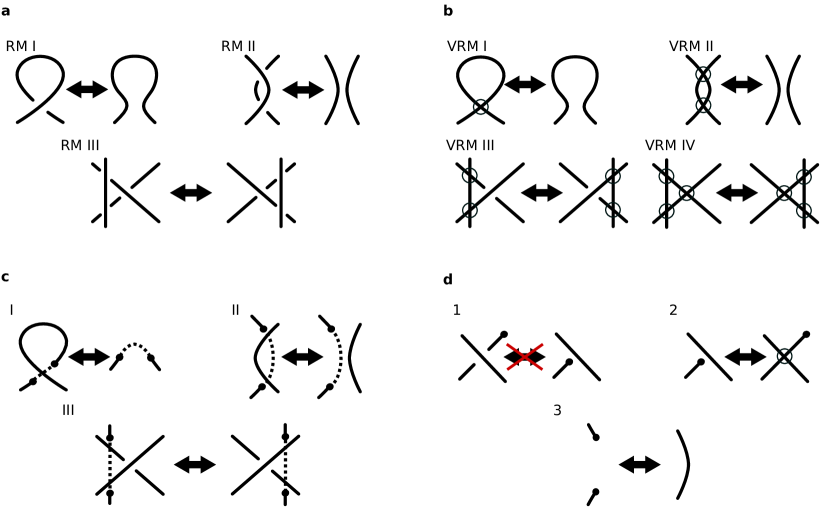
Supplementary Figure 1: Classical and virtual Reidemeister moves, and other algorithmic operations on open knot diagrams. The Reidemeister moves are local modifications to adjacent crossings of knot diagrams that do not change their topology. For each move, the rest of the curve (not shown) is assumed not to interact with the depicted region. A suitable combination of Reidemeister moves can (alongside planar isotopies) transform a given knot diagram to any other representing the same knot. (a) shows the classical Reidemeister moves involving only classical crossings, with standard labellings. (b) shows the virtual Reidemeister moves (virtual crossings are circled), which can involve changes in both classical and virtual crossings. (c) shows analogues of the virtual Reidemeister moves as closures of open curve diagrams with endpoints, in which case the Reidemeister changes clearly do not affect the topology resulting from virtual closure of the open strand. (d) highlights other relations that can be applied to open curve diagrams, whose application does not affect the virtual knot type resulting from virtual closure (disallowing moves 2 and 3 here reproduces the knot diagram relations of classical knotoids gugumcu16SI ). In (c) and (d), each endpoint of the open endpoints of the open curve is marked by a black circle.

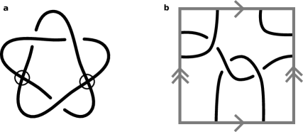
Supplementary Figure 2: Virtual knot $v3_{7}$, a virtual knot which cannot be formed from the closure of a projected open curve. The usual virtual knot diagram is shown in (a) while the presentation in (b) is depicted on the surface of a torus.

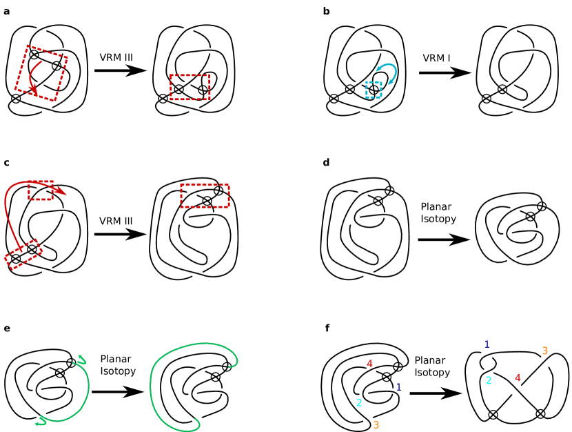
Supplementary Figure 3: Transformation between two depictions of the virtual knot $v4_{64}$. The initial conformation in (a) is that depicted as $v4_{64}$ in the virtual knot table of virtualknottableSI . This conformation could not arise from virtual closure of an open curve, as its virtual crossings do not lie sequentially along a single arc. An alternative presentation of this knot from the genus one table of andreevna14SI (labelled there as $4_{8}$), is shown in (f), and does have such a conformation, although it is difficult to see by eye that this is the same knot as $v4_{64}$. (b)-(e) show how (a) may be transformed to (f) by a combination of virtual Reidemeister moves and planar isotopies of the knot. In (e), the planar isotopy moving the green strand across the knot is not directly allowed by the virtual Reidemeister moves, but as the knot diagram is implicitly drawn on $\mathbb{S}^{2}$ this represents the strand passing ‘behind’ the sphere (or on the plane, passing through infinity). In general it is difficult to test whether two (virtual) knot diagrams can be related this way, hence the calculation of knot invariants which remove the need for diagrammatic manipulation.

Knot	$\Delta(-1)$	$\Delta(e^{2\pi i/3})$	$\Delta(i)$	$\Delta_{g}(-1,e^{2\pi i/3})$	$\Delta_{g}(-1,i)$	$\Delta_{g}(e^{2\pi i/3},i)$	$V(-1)$	$\Delta_{g}(s,t)$
$0_{1}$	1	1	1	0	0	0	1	0
$3_{1}$	3	2	1	0	0	0	3	0
$4_{1}$	5	4	3	0	0	0	5	0
$5_{1}$	5	1	1	0	0	0	5	0
$5_{2}$	7	5	3	0	0	0	6	0
$6_{1}$	9	7	4	0	0	0	9	0
$v2_{1}$	-	-	-	3	4	5	2	$s^{2}+s^{2}/t+st-s/t-t-1$
$v3_{2}$	-	-	-	3	4	5	4	$s+s/t+t-1/t-t/s-1/s$
$v4_{12}$	-	-	-	3	8	5	5	$s^{2}/t+s^{2}/t^{2}-st-s/t-2s/t^{2}-t^{2}+t-1/t+$ $1/t^{2}+2t^{2}/s+t/s+1/{st}-t^{2}/s^{2}-t/s^{2}$
$v4_{36}$	-	-	-	3	8	9	4	$t-1-1/t+1/t^{2}+t^{2}/s-2t/s+2/{st}-1/{st^{2}}-$ $t^{2}/s^{2}+t/s^{2}+1/s^{2}-1/{s^{2}t}$
$v4_{37}$	-	-	-	0	4	8	2	$s^{4}-s^{4}/t^{2}+s^{3}t+s^{3}/t^{2}-s^{2}t+s^{2}/t-st^{2}-s/t+t^{2}-1$
$v4_{43}$	-	-	-	7	8	9	5	$s^{3}+s^{3}/t+s^{2}t-s^{2}/t-st-s$
$v4_{64}$	-	-	-	3	4	0	4	$s^{2}/t+s^{2}/t^{2}-s/t-s/t^{2}+t^{2}/s+t/s-t^{2}/s^{2}-t/s^{2}$
$v4_{65}$	-	-	-	3	8	9	5	$-s^{2}t+s^{2}+s^{2}/t-s^{2}/t^{2}-st^{2}+2st-$ $2s/t+s/t^{2}+t^{2}-t-1+1/t$
$v4_{94}$	-	-	-	3	4	5	5	$s^{3}+s^{3}/t+s^{2}t-s^{2}/t-st-s$
$v4_{100}$	-	-	-	3	0	8	4	$s^{4}+s^{4}/t+s^{3}t-s^{3}/t-s^{2}t+s^{2}/t+st-s/t-t-1$

Supplementary Table 1: Table of numerical knot invariants for each knot shown in Fig. 2(a) and 2(b) of the main text. Included are $\Delta(t)$, the Alexander polynomial at the numerical values used, $\Delta_{g}(s,t)$ the generalised Alexander polynomial, both at the numerical values used and the full symbolic expression, and $V(q)$ the Jones polynomial. Virtual knots have no Alexander polynomial and so these columns are omitted. In the cases where chiral mirrors give different knots, only one mirror is given.

Supplementary Note 1: Topological Background

Classical Knot Theory

In this Supplementary Note we summarise some extended details of mathematical knot theory as used in deriving the results of the main text. Further details can be found in standard elementary texts adams94SI ; rolfsen76SI ; sossinsky02SI .

Classical knot theory deals with embeddings of the circle, $S^{1}$ (i.e. closed, non-intersecting curves), in three-dimensional space $\mathbb{R}^{3}$. Any given embedding has a distinct knot type, which is invariant under ambient isotopies (it may change only when the curve passes through itself). It is usual to represent knots using a 2-dimensional planar knot diagram, which can be thought of as a plane projection of the three-dimensional space curve, annotated with the extra information of which strand passes over the other at each self-intersection of the diagram (called a crossing). All the information about the three-dimensional knot type is contained in such a diagram, and smooth deformations (i.e. ambient isotopies) of the three-dimensional space curve lead to smooth isotopies of the knot diagram, which may change the configuration of the crossings. In two-dimensional knot diagrams, the changes are represented by combinations of Reidemeister moves as in Supplementary Fig. 1(a); applying these local moves in conjunction with planar isotopies of the knot diagram can transform between any two diagrammatic representations of the same knot, and equivalently any ambient isotopy of a closed three-dimensional space curve is corresponds to a combination of planar isotopies and Reidemeister moves in any projection of the knot.

The standard tabulations of knots, in knot tables as discussed in the main text, are ordered according to their minimal crossing number $n$ – the smallest number of crossings a diagram of the knot can have. For instance, the trivial circle can be projected to a plane without self intersection (i.e. no crossings), and so has minimal crossing number $n=0$ and is labelled $0_{1}$. There are no knots with $n=2$, and one with $n=3$, the trefoil knot, denoted $3_{1}$. The labelling $n_{m}$ continues, where $m$ is an arbitrary index amongst knots with the same $n$. These labels are standard, following original tabulations up to $n=10$ published over 100 years ago, with more recent extensions using consistent indices rolfsen76SI ; knotatlasSI ; knotinfoSI . Some simple knots from these tabulations are shown in Fig. 2(a). $0_{1}$ (the unknot), then $3_{1}$, $4_{1}$, etc. The knots appearing in knot tables are prime knots; composite knots, made up of two or more prime knots tied in the same curve, are also possible and are tabulated according to the composition of their prime factors adams94SI . All the tools of knot theory apply equally to composite knots, but they do not occur significantly in any known protein chain, and are not considered further here.

It is natural to follow the curve of a knot, which endows an orientation to the knot (choosing an orientation is an arbitrary choice that does not affect the results of topological calculations). Observing the relative orientation of the strands at a crossing determines the sign of the crossing, either positive or negative. A crossing has the same sign even if the curve’s orientation is reversed. The minimal diagram of a figure-8 knot $4_{1}$ has two positively signed crossings and two negatively signed, and in fact is isotopic to its mirror image. On the other hand, all three crossings of the minimal trefoil knot $3_{1}$ have the same sign, and are all reversed on its mirror image. Knots such as the trefoil are thus chiral knots, and this chirality not directly represented in the tabulation (i.e. there are two enantiomeric trefoil knots which cannot be be smoothly deformed into one another). Other chiral knots are $5_{1}$, $5_{2}$ and $6_{1}$ in Fig. 2(a) of the main text; the others are achiral. We do not distinguish between chiral knot pairs in our analysis, although knot invariant quantities such as used to distinguish knots below could be used to do so.

In practice the knot type of a space curve is determined as follows. First the curve is projected to a 2D knot diagram, which contains all the topological information in its ordered set of signed crossings along the curve. Several topological notations representing this information are standard adams94SI ; rolfsen76SI ; we use below the Gauss code, constructed from an arbitrary starting point and orientation for the curve. As each new crossing is encountered along the curve, it is labelled $1,2,\ldots$ in order as it is encountered. The Gauss code is the ordered list of these crossing numbers as they occur along the curve, together with whether the curve passes over or under the intersecting strand, represented by using a positive number in the former case and negative in the latter (this is not the same as the crossing sign); each crossing must be encountered exactly twice before reaching the original starting point, once positive and once negative. For instance, a Gauss code for a minimal diagram of the trefoil knot $3_{1}$ is $1,{-2},3,{-1},2,{-3}$, and for a minimal figure-8 knot $4_{1}$ is $1,{-2},3,{-1},4,{-3},2,{-4}$. It is obvious that changing the starting point on the curve cyclically permutes the crossings encountered, but all the Gauss codes obtained this way, or by changing numeric labels (as long as each crossing retains a unique label) represent the same knot diagram. The Gauss code written in this way also does not specify the chirality of the original three-dimensional curve, this information is contained in the local twisting of the two strands around one another and is sometimes included in extended Gauss code notations. Crossings which can be removed by Reidemeister moves I and II can be easily identified in a Gauss code; if crossing $k$ occurs adjacent to itself, $\pm k,\mp k$ then it can be removed by Reidemeister move I, and if $\pm k,\pm k+1,\ldots\mp k,\mp k+1$ (or $\mp k+1,\mp k$), then crossings $k,k+1$ can be removed by Reidemeister move II.

All knot diagrams can be represented by Gauss codes, but in fact not all Gauss code sequences represent knot diagrams; for instance, the sequence $1,-2,-1,2$ appears to be a consistent Gauss code of only two crossings, which cannot be simplified by Reidemeister moves, and no knot has $n=2$. On attempting to draw a diagram with this code, one finds it would be necessary for there to be one extra crossing to allow the curve to return to its starting point. In fact, this is the Gauss code of the open diagram shown in Fig. 2 (e) of the main text, and Gauss codes for open diagrams, and their relation to virtual knots, is the subject of the next section.

It can be practically difficult to calculate the knot type of a diagram coming from a projection of a complicated 3D space curve, which may have many more crossings than its minimal number $n$. These crossings would represent local geometrical or biochemical features that do not affect the overall knot type; the knot diagrams found from closures of protein backbones often contain several hundred crossings. Our knot identification proceeds first by algorithmic simplification via removal of crossings, repeatedly applying Reidemeister moves I and II where they would remove crossings locally (Supplementary Fig. 1(a)), as discussed above. There is no known efficient method to produce minimal knot diagrams in this way as Reidemeister move III may also be essential to simplify the diagram but does not directly reduce the crossing number. In the case of protein backbones, this occasionally produces minimal diagrams but in most cases tens to hundreds of crossings remain.

The knot types of the simplified diagrams are calculated using knot invariants, quantities that depend only on the knot type but are calculated from the geometrical information of the curve, i.e. they can be calculated from only the information in a Gauss code and their value is invariant to Reidemeister moves. Much of mathematical knot theory is devoted to the study of knot invariants, and many types are known. For instance, the minimal crossing number discussed above is a knot invariant adams94SI , but there is no simple algorithm to calculate it directly from a presentation of a knot. The minimal crossing number also demonstrates that most invariants do not perfectly distinguish knots adams94SI , as multiple different knots can clearly have the same number of crossings in their minimal projections; for instance, both $5_{1}$ and $5_{2}$ in Fig. 2(a) have $n=5$. More discriminatory invariants exist but are generally relatively difficult to calculate.

For knot identification we use knot invariants that can be calculated efficiently (ideally in low order polynomial time in the number of crossings), while still discriminating knots sufficiently well. In particular, we choose invariants which leave no ambiguity between the knots common on closure of proteins such as those in Fig. 2(a) of the main text. Some protein closures produce complex knots whose knot type cannot be uniquely identified using these efficient invariants, but these occur only rarely and do not impact our analysis. For classical knots, we employ only the Alexander polynomial $\Delta(t)$, which can be found as the determinant of a matrix whose rows and columns relate to the crossings of a projected diagram and can be easily constructed from a Gauss code orlandini07SI . Computing symbolic matrices numerically is relatively slow, and we instead use the values of $|\Delta(t)|$ evaluated at roots of unity $t=-1$, $t=\exp(2\pi i/3)$ and $t=i$, such that the calculation can be performed using floating point arithmetic (this does not introduce appreciable error). Each of these is individually a lesser knot invariant, but together they have discriminatory power comparable to the full Alexander polynomial up to at least 11 minimal crossings (certainly sufficient for the relatively simple knots that appear in protein chains).

Many knot invariants, including the Alexander polynomial, are available from standard online resources including the Knot Atlas knotatlasSI for all knots with up to 15 crossings, and KnotInfo knotinfoSI for a wider selection of invariants up to 12 crossings. Supplementary Table 1 shows values of $\Delta(t)$ at the roots of unity used above, for each of the simple knots that appear most commonly in protein chains.

Virtual Knots

Virtual knots are an extension to the theory of classical knots kauffman99SI which classify all topological objects formed of ordered crossings, which generalises the theory of knot diagrams while keeping a sense of isotopy through Reidemeister moves. In particular, this includes those orderings which cannot be realised as plane projections of (closed) space curves in $\mathbb{R}^{3}$. They can be thought of as the objects represented by the set of all Gauss codes, including sequences such as $1,-2,-1,2$, which does not correspond to any closed knot diagram, as discussed above. In this sense, they provide a natural framework to describe open diagrams, with endpoints that cannot directly be joined, so do not correspond to classical knots but have knot-like structure in their sequence of ordered crossings.

Many concepts from classical knot theory naturally generalise to virtual knots, such as the distinction between prime and composite virtual knots (including composites with classical and virtual components). Virtual knots are tabulated according to their minimum classical crossing number $n$ virtualknottableSI , and they are denoted here as $vn_{m}$, following the tabulation of virtualknottableSI , as described in the main text. The simplest nontrivial virtual knot, $v2_{1}$, has $n=2$, and Gauss code $1,-2,-1,2$. There are many more prime virtual knots for $n\geq 2$ than classical knots; complete tabulations only extend to virtual knots up to $n=5$. There are also up to three distinct chiral symmetric partners of a given virtual knot (compared to at most one partner of opposite chirality for classical knots): a mirror reflection of the diagram preserving the classical crossing signs, an inversion where all classical crossing signs are flipped, and the combination of both mirrors. As with the classical knots, we identify all chiral partners of the same virtual knot type as equivalent.

kauffman99SI presents two further equivalent interpretations of virtual knots, both of which illustrate properties discussed in the main text. The first, convenient for diagrammatic representation, draws virtual knots as classical knot diagrams (without endpoints) but augmented with an additional crossing type at self intersection, the virtual crossing, denoted by a circle around the intersection (e.g. Fig. 2(b) of the main text). Virtual crossings do not have a sign and do not contribute to topological calculations, so the Gauss code follows only by considering the virtual diagram’s classical crossings and ignoring virtual crossings entirely. In such virtual diagrams, virtual crossings can be manipulated by suitable generalisations of the classical Reidemeister moves, which can affect the configuration of virtual and classical crossings but do not change the virtual knot type; these moves are shown in Supplementary Fig. 1(b). In particular, virtual Reidemeister moves I and II can change the number of virtual crossings, and minimal virtual crossing number is an invariant of virtual knots; those with minimum virtual crossing number zero are the classical knots, which make up a subset of the generalised, virtual knots. We describe a knot here as virtual if the minimum number of virtual crossings is greater than zero.

The other interpretation of virtual knots is as closed knot diagrams drawn on surfaces with topology different to the standard plane of projection (equivalent to its one-point compactification, the 2-sphere), i.e. drawn on handlebodies with nonzero genus. Any virtual knot can be drawn as a knot diagram without virtual crossings on a surface of sufficiently high genus kauffman99SI . The virtual crossings previously described are then interpreted as a consequence of projection from the handlebody to a plane, in which case the virtual crossings are intersections of two strands from different bridges of the handlebody (likewise, a virtual knot diagram with virtual crossings can be made a knot diagram on a handlebody by replacing each virtual crossing with a handle which one strand passes ‘along’ and the other ‘under’ the handle). The minimum genus of any handlebody on which the virtual knot can be drawn defines the virtual genus (hereafter referred to as the genus, although this is distinctly different to the genus referred to in classical knot theory adams94SI ) of the virtual knot, and is therefore 0 for classical knots while any virtual knot must have genus at least 1.

Here, we are considering 2D open diagrams as virtual knots, and these interpretations of virtual knots relate directly to virtual closure of open diagrams (formed by projection of open 3D chains) considered in the main text. The virtual closure of an open knot diagram corresponds to adding a closing arc between the open diagram’s endpoints, where all intersections of this arc with the rest of the diagram make virtual crossings. All closure arcs are equivalent as they may be transformed to one another using virtual Reidemeister moves; the Gauss code only depends on the original open diagram, and does not change when the virtual crossings are altered. In fact, the virtual Reidemeister moves can be interpreted in terms of the endpoints of open diagrams, shown in Supplementary Fig. 1(c) in which the moves are effectively equivalent to different choices of closure.

It is possible to consider the open diagram in these terms alone (i.e. the open diagram is subject only to the three classical Reidemeister moves, but the endpoints are forbidden to pass over or under a strand creating (or removing) new crossings, Supplementary Fig. 1(d), otherwise the open diagram could be untangled to the trivial open curve); this would produce a classical knotoid turaev12SI , a topological object that encodes information about the topology of the open curve, but whose classes are not isomorphic to the virtual knots gugumcu16SI . Representing knotoids by virtual knots loses some information – for instance it may not be clear, from a virtual diagram, which arc at a virtual crossing is the virtual closure arc (i.e. multiple, distinct knotoids give the same virtual knot). However, in our analysis, we opt to work with virtual knots since their tabulation, invariants and other properties are a lot better developed and understood than for knotoids, and therefore are more convenient for application without new mathematics. Only a small amount of information is apparently lost through the ambiguity of knotoids as virtual knots, which does not appear to unduly limit topological analysis; this can be considered as a similar simplification to ignoring the chirality of knots.

Since all the virtual crossings resulting from virtual closure necessarily occur sequentially along the same arc, the genus of virtual knots obtained by closing open diagrams is at most one. That is, all the virtual crossings of the diagram may be removed by adding a single handle to the surface on which it is drawn, in between the endpoints of the open curve, and along which the closing arc runs. Not all genus one virtual knots can be represented in this way such that their virtual crossings occur sequentially; an example is shown in Supplementary Fig. 2(a), whose two virtual crossings can never be adjacent even under the application of (virtual) Reidemeister moves, although the knot can be drawn on a genus one surface sich as the planar diagram shown in Supplementary Fig. 2(b). The class of virtual knots that can be obtained from closures of open knot diagrams is therefore subset of genus one virtual knots, whose minimal presentations pass around the torus exactly once in one generator direction, and at least once in the other. This is related to the homology of the curve as drawn on a genus one handlebody: for any such diagram we can associate an index with the number of times a curve wraps around the torus in each direction, and for a virtual knot these homology indices must be of the form $(\pm 1,j)$ for $|j|\geq 1$ (although this condition is not on its own sufficient due to the presence of more complex topologies with the same overall homology). We therefore refer to the virtual knots appearing as virtual closures of open curves as minimally genus one virtual knots.

The virtual knots of genus one were studied and tabulated by andreevna14SI . Their description involves a virtual knot invariant that is a generalisation of the Kauffman bracket polynomial with two variables $a$ and $x$, calculated from the virtual knot diagram as drawn on the 2-torus. Each possible bracket smoothing of this diagram, $s$, is associated with a factor of $x^{\delta(s)}$, where $\delta(s)$ is the number of circles of nontrivial homology in a given smoothing. The polynomials for all minimally genus 1 virtual knots therefore have the form $xf(a)$, where $f(a)$ is a function of the knot which does not depend on $x$, and this property therefore allows all minimally genus one knots to be readily identified. The minimally genus one virtual knots of up to $n=4$, in the genus one table andreevna14SI are, in the notation of that work: $2_{1}$, $3_{1}$, $4_{1}$, $4_{2}$, $4_{3}$, $4_{6}$, $4_{7}$, $4_{8}$ and $4_{9}$. In the complete virtual knot table virtualknottableSI , the diagrams which are explicitly minimally genus one are: $v2_{1}$, $v3_{2}$, $v4_{12}$, $v4_{43}$, $v4_{65}$, $v4_{94}$ and $v4_{100}$. After comparing knot invariants between the two tabulations, we were unable to find a partner in andreevna14SI for the minimally genus one $v4_{12}$ (i.e. it appears to be an erroneous omission). Thus, from  andreevna14SI we could identify three further minimally genus one virtual knots than the complete table, with this property also confirmed via the Kauffman bracket method; these correspond to $v4_{36}$, $v4_{37}$ and $v4_{64}$ in virtualknottableSI (up to chiral mirrors). This relationship would be difficult to see by direct inspection of the diagram, and Supplementary Fig. 3 demonstrates the equivalence of the different presentations for $v4_{64}$, via a combination of virtual Reidemeister moves and planar isotopies. All other minimally genus one examples agree in the two tables, and we believe that this completes the full set of minimally genus one virtual knots with up to four classical crossings.

Just as with classical knots, we identify virtual knot types by calculating virtual knot invariants (which are, in many cases, generalisations of classical invariants, such as the Kauffman bracket polynomial already discussed). Typically it is more computationally expensive to discriminate virtual knots than classical knots of the same minimum crossing number $n$. The basic procedure of invariant calculation is similar to that of classical knots, although now virtual crossings may also be algorithmically removed via virtual Reidemeister moves I and II. This does not directly affect the classical crossings, but may allow more of them to be removed. The Alexander polynomial has a number of extensions in virtual knot theory; we work with the two variable generalised Alexander polynomial $\Delta_{g}(s,t)$ kauffman03SI . As with classical knots, the calculation is significantly faster evaluated at constant values of $s$ and $t$, and we use the combinations ($s=-1$, $t=e^{2\pi i/3})$), ($s=-1$, $t=i$) and ($s=e^{2\pi i/3}$, $t=i$). However, in contrast to classical knots, the generalised Alexander polynomial is not enough to distinguish the two simplest virtual knots possible from open curves, $v2_{1}$ and $v3_{2}$, as well as some other simple virtual knots (the next are $v4_{36}$ and $v4_{65}$, but although they are relatively simple these do not contribute significantly to any of our analysis). When necessary (but primarily in the case of $v2_{1}$ and $v3_{2}$), we resolve this ambiguity using the Jones polynomial $V(q)$ jones85SI , which is a classical knot invariant that extends to virtual knots without modification. Since computation of the Jones polynomial takes exponential time in the number of crossings adams94SI ; knotatlasSI , we compute it only at the constant $q=-1$ (sufficient to distinguish $v2_{1}$, $v3_{2}$, etc.), and only when our chosen values of $\Delta_{g}(s,t)$ are not sufficiently discriminatory to identify the virtual knot.

Virtual knot invariants for each of the virtual knots with up to four classical crossings can be found in the online knot table of virtualknottableSI or, for the Kauffman bracket variant explained above, in andreevna14SI . Supplementary Table 1 further shows the values of $\Delta_{g}$ and $V$ for each of the minimally genus one virtual knots in these tables, which together are clearly sufficient to distinguish all relevant knot types.

References

- (1) Branden, C. I. & Tooze, J. Introduction to Protein Structure, chap. 1 (Garland Science, 1998).
- (2) Adams, C. C. The Knot Book (American Mathematical Society, 1994).
- (3) Millett, K. C., Rawdon, E. J., Stasiak, A. & Sulkowska, J. L. Identifying knots in proteins. Biochemical Society Transactions 41, 533–7 (2013).
- (4) Tubiana, L., Orlandini, E. & Micheletti, C. Probing the entanglement and locating knots in ring polymers: a comparative study of different arc closure schemes. Progress of Theoretical Physics Supplements 191, 192–204 (2011).
- (5) Berman, H. M. et al. The Protein Data Bank. Nucleic Acids Research 28, 235–42 (2000). URL www.rcsb.org.
- (6) Jamroz, M. et al. Knotprot: a database of proteins with knots and slipknots. Nucleic Acids Research 43, D306–14 (2014).
- (7) Lua, R. C. & Grosberg, A. Y. Statistics of knots, geometry of conformations, and evolution of proteins. PLOS Computational Biology 2, e45 (2006).
- (8) Mallam, A. L. & Jackson, S. E. Knot formation in newly translated proteins is spontaneous and accelerated by chaperonins. Nature Chemical Biology 8, 147–53 (2012).
- (9) Faísca, P. F. N. Knotted proteins: A tangled tale of structural biology. Computational and Structural Biotechnology Journal 13, 459–68 (2015).
- (10) Lim, N. C. H. & Jackson, S. E. Molecular knots in biology and chemistry. Journal of Physics: Condensed Matter 27, 354101 (2015).
- (11) James, P. et al. The structure of a tetrameric -carbonic anhydrase from Thermovibrio ammonificans reveals a core formed around intermolecular disulfides that contribute to its thermostability. Acta Crystallographica Section D: Biological Crystallography 70, 2607–18 (2014).
- (12) Haglund, E. et al. Pierced lasso bundles are a new class of knot-like motifs. PLOS Computational Biology 10, e1003613 (2014).
- (13) Dabrowski-Tumanski, P., Niemyska, W., Pasznik, P. & Sulkowska, J. I. Lassoprot: server to analyze biopolymers with lassos. Nucleic Acids Research 44, W383–9 (2016).
- (14) Flapan, E. & Heller, G. Topological complexity in protein structures. Molecular Based Mathematical Biology 3, 23–42 (2015).
- (15) Cao, Z., Roszak, A. W., Gourlay, L. J., Lindsay, J. G. & Isaacs, N. W. Bovine mitochondrial peroxiredoxin III forms a two-ring catenane. Structure 13, 1661–4 (2005).
- (16) Boutz, D. R., Cascio, D., Whitelegge, J., Perry, L. J. & Yeates, T. O. Discovery of a thermophilic protein complex stabilized by topologically interlinked chains. Journal of Molecular Biology 368, 1332–44 (2007).
- (17) McDonald, N. Q. & Hendrickson, W. A. A structural superfamily of growth factors containing a cystine knot motif. Cell 73, 421–4 (1993).
- (18) Kauffman, L. H. Virtual knot theory. European Journal of Combinatorics 20, 663–90 (1999).
- (19) Rolfsen, D. (ed.) Knots and Links (AMS Chelsea Publishing, 1976).
- (20) Hoste, J., Thistlethwaite, M. & Weeks, J. The first knots. The Mathematical Intelligencer 20, 33–48 (1998).
- (21) The Knot Atlas. URL http://katlas.org. Accessed Sep 2016.
- (22) Cha, J. C. & Livingston, C. Knotinfo: Table of knot invariants. URL http://www.indiana.edu/~knotinfo. Accessed Sep 2016.
- (23) Green, J. & Bar-Natan, D. A table of virtual knots. URL https://www.math.toronto.edu/drorbn/Students/GreenJ/. Accessed Sep 2016, last updated Aug 2004.
- (24) Turaev, V. Knotoids. Osaka Journal of Mathematics 49, 195–223 (2012).
- (25) Gügümcü, N. & Kauffman, L. H. New invariants of knotoids. arXiv:1602.03579 (2016).
- (26) Wang, F. et al. Understanding molecular recognition of promiscuity of thermophilic methionine adenosyltransferase sMAT from Sulfolobus solfataricus. FEBS Journal 281, 4224–39 (2014).
- (27) Taylor, A. J. & Dennis, M. R. Vortex knots in tangled quantum eigenfunctions. Nature Communications 7, 12346 (2016).
- (28) Kauffman, L. H. & Radford, D. E. Bioriented quantum algebras and a generalized Alexander polynomial for virtual links. In Diagrammatic Morphisms and Applications, vol. 318 of Contemporary Mathematics, 113–40 (American Mathematical Society, 2003).
- (29) Jones, V. F. R. A polynomial invariant for knots and links via Von Neumann algebras. Bulletin of the American Mathematical Society 12, 103–11 (1985).
- (30) Kauffman, L. H. State models and the Jones polynomial. Topology 26, 395–407 (1987).
- (31) Rakhmanov, E. A., Saff, E. B. & Zhou, Y. M. Minimal discrete energy on the sphere. Mathematical Research Letters 1, 647–62 (1994).
- (32) Lai, Y. L., Chen, C. C. & Hwang, J. K. pKNOT: the protein KNOT web server. Nucleic Acids Research 35, W420–4 (2007).
- (33) Kolesov, G., Virnau, P., Kardar, M. & Mirny, L. A. Protein knot server: detection of knots in protein structures. Nucleic Acids Research 35, W425–8 (2007).
- (34) Bellini, D. & Papiz, M. Z. Dimerization properties of the RpBphP2 chromophore-binding domain crystallized by homologue-directed mutagenesis. Acta Crystallographica Section D: Biological Crystallography 68, 1058–66 (2012).
- (35) Sugimoto, K. et al. Molecular mechanism of strict substrate specificity of an extradiol dioxygenase, DesB, derived from Sphingobium sp. SYK-6. PLOS ONE 9, e92249 (2014).
- (36) Oualid, F. E. et al. Chemical synthesis of ubiquitin, ubiquitin-based probes, and diubiquitin. Angewandte Chemie International Edition 49, 10149–53 (2010).
- (37) Wischeler, J. S. et al. Stereo- and regioselective azide/alkyne cycloadditions in carbonic anhydrase II via tethering, monitored by crystallography and mass spectrometry. Chemistry – A European Journal 17, 5842–51 (2011).
- (38) Falconer, K. Fractal Geometry: Mathematical Foundations and Applications, chap. 3 (John Wiley & Sons, 1997).
- (39) Orlandini, E. & Whittington, S. G. Statistical topology of closed curves: Some applications in polymer physics. Reviews of Modern Physics 79, 611–42 (2007).
- (40) Flory, P. J. Principles of Polymer Chemistry (Cornell University Press, 1953).
- (41) Cantarella, J., Deguchi, T. & Shonkwiler, C. Probability theory of random polygons from the quaternionic viewpoint. Communications of Pure and Applied Analytics 67, 1658–99 (2014).
- (42) Lua, R., Borovinskiy, A. L. & Grosberg, A. Y. Fractal and statistical properties of large compact polymers: a computational study. Polymer 45, 717–31 (2004).
- (43) Marenduzzo, D., Micheletti, C., Orlandini, E. & D WSumners, D. Topological friction strongly affects viral DNA ejection. Proceedings of the National Academy of Sciences 110, 20081–6 (2013).
- (44) Diao, Y., Ernst, C. & Ziegler, U. Random walks and polygons in tight confinement. Journal of Physics: Conference Series 544, 012017 (2014).
- (45) Orlandini, E. & Micheletti, C. Knotting of linear DNA in nano-slits and nano-channels: a numerical study. Journal of Biological Physics 39, 267–75 (2013).
- (46) Micheletti, C. & Orlandini, E. Numerical study of linear and circular model DNA chains confined in a slit: metric and topological properties. Macromolecules 45, 2113–21 (2012).
- (47) Sulkowska, J. L., Rawdon, E. J., Millett, K. C., Onuchic, J. N. & Stasiak, A. Conservation of complex knotting and slipknotting patterns in proteins. Proceedings of the National Academy of Sciences 109, E1715–23 (2012).
- (48) Berman, H., Henrick, K. & Nakamura, H. Announcing the worldwide Protein Data Bank. Nature Structural & Molecular Biology 10, 980 (2003).
- (49) Bakan, A., Meireles, L. M. & Bahar, I. ProDy: Protein Dynamics Inferred from Theory and Experiments. Bioinformatics 27, 1575–7 (2011).
- (50) McNicholas, S., Potterton, E., Wilson, K. S. & Noble, M. E. M. Presenting your structures: the CCP4mg molecular-graphics software. Acta Crystallographica Section D: Biological Crystallography 67, 386–94 (2011).

References

- (1) Gügümcü, N. & Kauffman, L. H. New invariants of knotoids. arXiv:1602.03579 (2016).
- (2) Green, J. & Bar-Natan, D. A table of virtual knots. URL https://www.math.toronto.edu/drorbn/Students/GreenJ/. Accessed Sep 2016, last updated Aug 2004.
- (3) Andreevna, A. A. & Matveev, S. V. Classification of genus 1 virtual knots having at most five classical crossings. Journal of Knot Theory and Its Ramifications 23, 1450031 (2014).
- (4) Adams, C. C. The Knot Book (American Mathematical Society, 1994).
- (5) Rolfsen, D. (ed.) Knots and Links (AMS Chelsea Publishing, 1976).
- (6) Sossinsky, A. Knots: mathematics with a twist (Harvard University Press, 2002).
- (7) The Knot Atlas. URL http://katlas.org. Accessed Sep 2016.
- (8) Cha, J. C. & Livingston, C. Knotinfo: Table of knot invariants. URL http://www.indiana.edu/~knotinfo. Accessed Sep 2016.
- (9) Orlandini, E. & Whittington, S. G. Statistical topology of closed curves: Some applications in polymer physics. Reviews of Modern Physics 79, 611–42 (2007).
- (10) Kauffman, L. H. Virtual knot theory. European Journal of Combinatorics 20, 663–90 (1999).
- (11) Turaev, V. Knotoids. Osaka Journal of Mathematics 49, 195–223 (2012).
- (12) Kauffman, L. H. & Radford, D. E. Bioriented quantum algebras and a generalized Alexander polynomial for virtual links. In Diagrammatic Morphisms and Applications, vol. 318 of Contemporary Mathematics, 113–40 (American Mathematical Society, 2003).
- (13) Jones, V. F. R. A polynomial invariant for knots and links via Von Neumann algebras. Bulletin of the American Mathematical Society 12, 103–11 (1985).