Brownian yet non-Gaussian diffusion: from superstatistics to subordination of diffusing diffusivities

Abstract

A growing number of biological, soft, and active matter systems are observed to exhibit normal diffusive dynamics with a linear growth of the mean squared displacement, yet with a non-Gaussian distribution of increments. Based on the Chubinsky-Slater idea of a diffusing diffusivity we here establish and analyze a minimal model framework of diffusion processes with fluctuating diffusivity. In particular, we demonstrate the equivalence of the diffusing diffusivity process with a superstatistical approach with a distribution of diffusivities, at times shorter than the diffusivity correlation time. At longer times a crossover to a Gaussian distribution with an effective diffusivity emerges. Specifically, we establish a subordination picture of Brownian but non-Gaussian diffusion processes, that can be used for a wide class of diffusivity fluctuation statistics. Our results are shown to be in excellent agreement with simulations and numerical evaluations.

I Introduction

Thermally driven diffusive motion belongs to the fundamental physical processes. To a big extent inspired by the groundbreaking experiments of Robert Brown in the 1820ies brown the theoretical foundations of the theory of diffusion were then laid by Einstein, Sutherland, Smoluchowski, and Langevin between 1905 and 1908 einstein ; sutherland ; smoluchowski ; langevin . On their basis novel experiments, such as the seminal works by Perrin and Nordlund perrin ; nordlund , in turn delivered ever better quantitative information on molecular diffusion as well as the atomistic nature of matter. Typically, we now identify two fundamental properties with Brownian diffusive processes: (i) the linear growth in time of the mean squared displacement (MSD)

$$\langle\mathbf{r}^{2}(t)\rangle=\int_{-\infty}^{\infty}\mathbf{r}^{2}P(\mathbf{r},t)d\mathbf{r}=2dDt$$ (1)

typically termed normal (Fickian) diffusion. Here $d$ denotes the spatial dimension and $D$ is called the diffusion coefficient. (ii) The second property is the Gaussian shape

$$P(\mathbf{r},t)=\frac{1}{(4\pi Dt)^{d/2}}\exp\left(-\frac{\mathbf{r}^{2}}{4Dt}\right)$$ (2)

of the probability density function to find the diffusing particle at position $\mathbf{r}$ at some time $t$ vankampen . From a more mathematical viewpoint the Gaussian emerges as limit distribution of independent, identically distributed random variables (the steps of the random walk) with finite variance and in that sense assumes a universal character gnedenko .

Deviations from the linear time dependence (1) are routinely observed. Thus, modern microscopic techniques reveal anomalous diffusion with the power-law dependence $\langle\mathbf{r}^{2}(t)\rangle\simeq t^{\alpha}$ of the MSD, where according to the value of the anomalous diffusion exponent we distinguish subdiffusion for $0<\alpha<1$ and superdiffusion with $1<\alpha<2$ bouchaud ; report ; pccp ; bba ; hoefling . Examples for subdiffusion of passive molecular and submicron tracers abound in the cytoplasm of living biological cells golding ; goldinga ; goldingb and in artificially crowded fluids banks , as well as in quasi two-dimensional systems such as lipid bilayer membranes membranes ; membranesa ; membranesb ; membranesc . Superdiffusion is typically associated with active processes and also observed in living cells elbaum . Anomalous diffusion processes arise due to the loss of independence of the random variables, divergence of the variance of the step length or the mean of the step time distribution, as well as due to the tortuosity of the embedding space. The associated probability density function of anomalous diffusion processes may have both Gaussian and non-Gaussian shapes bouchaud ; report ; pccp .

A new class of diffusive dynamics has recently been reported in a number of soft matter, biological and other complex systems: in these processes the MSD is normal of the form (1), however, the probability density function $P(\mathbf{r},t)$ is non-Gaussian, typically characterized by a distinct exponential shape

$$P(\mathbf{r},t)\simeq\exp\left(-\frac{|\mathbf{r}|}{\lambda(t)}\right),$$ (3)

with the decay length $\lambda(t)=\sqrt{Dt}$ granick . This form of the probability density function is also sometimes called a Laplace distribution. The Brownian yet non-Gaussian feature appears quite robustly in a large range of systems, including beads diffusing on lipid tubes wang or in networks wang ; gels , tracer motion in colloidal, polymeric, or active suspensions susp , in biological cells bio , as well as the motion of individuals in heterogeneous populations such as nematodes hapca . For additional examples see bng ; bnga ; bngb ; bngc and the references in granick ; gary ; klsebastian .

How can this combination of normal, Brownian scaling of the mean squared displacement be reconciled with the existence of a non-Gaussian probability density function? One argument not brought forth in the discussion of anomalous diffusion above is the possibility that the random variables making up the observed dynamics are indeed not identically distributed. This fact can be introduced in different ways. First, Granick and co-workers wang as well as Hapca et al. hapca employed distributions of the diffusivity of individual tracer particles to explain this remarkable behavior: indeed, averaging the Gaussian probability density function (2) for a single diffusivity $D$ over the exponential distribution $p_{D}(D)=\langle D\rangle^{-1}\exp(-D/\langle D\rangle)$ with the mean diffusivity $\langle D\rangle$, the exponential form (3) of the probability density function emerges gary ; hapca . In fact, this idea of creating an ensemble behavior in terms of distributions of diffusivities of individual tracer particles is analogous to the concept of superstatistical Brownian motion: based on two statistical levels describing, respectively, the fast jiggly dynamics of the Brownian particle and the slow environmental fluctuations with spatially local patches of given diffusivity this concept demonstrates how non-Gaussian probability densities arise physically beck . In what follows we refer to averaging over a diffusivity distribution $p_{D}(D)$ as superstatistical approach. An important additional observation from experiments that cannot be explained by the superstatistical approach is that “the distribution function will converge to a Gaussian at times greater than the correlation time of the fluctuations” granick . This is impressively demonstrated, for instance, in Fig. 1C in wang . This crossover cannot be explained by the superstatistical approach. At the same time the normal-diffusive behavior is not affected by the crossover between the shapes of the distribution.

Second, Chubinsky and Slater came up with the diffusing diffusivity model, in which the diffusion coefficient of the tracer particle evolves in time like the coordinate of a Brownian particle in a gravitational field gary . For short times they indeed find an exponential form (3). At long times, they demonstrate from simulations that the probability density function crosses over to a Gaussian shape. Jan and Sebastian formalize the diffusing diffusivity model in an elegant path integral approach, which they explictly solve in two spatial dimensions klsebastian . Their results are consistent with those of Ref. gary .

Here we introduce a simple yet powerful minimal model for diffusing diffusivities, based on the concept of subordination. Based on a double Langevin equation approach our model is fully analytical, providing an explicit solution for the probability density function in Fourier space. The inversion is easily feasible numerically, and we demonstrate excellent agreement with simulations of the underlying stochastic equations. Moreover, we provide the analytical expressions for the asymptotic behavior at short and long times, including the crossover to Gaussian statistics, and derive explicit results for the kurtosis of the probability density function. The bivariate Fokker-Planck equation for this process and its connection to the subordination concept are established. Finally, we show that at times shorter than the diffusivity correlation time our analytical results are fully consistent with the superstatistical approach. Our approach has the distinct advantage that it is amenable to a large variety of different fluctuating diffusion scenarios.

In what follows we first formulate the coupled Langevin equations for the diffusing diffusivity model. Section 3 then introduces the subordination concept allowing us to derive the exact form of the subordinator as well as the Fourier image of the probability density function. The Brownian form of the MSD is demonstrated and the short and long time limits derived. Moreover, the connection to the superstatistical approach is made. The kurtosis quantifying the non-Gaussian shape of the probability density function is derived. In section 4 the bivariate Fokker-Planck equation for the joint probability density function $P(x,D,t)$ is analyzed, before drawing our conclusions in section 5. Several Appendices provide additional details.

II Superstatistical approach to Brownian yet non-Gaussian diffusion

As mentioned above, it was suggested by Granick and coworkers granick as well as by Hapca et al. hapca that the Laplace distribution

$$P(x,t)=\frac{1}{\sqrt{4\langle D\rangle t}}\exp\left(-\frac{|x|}{(\langle D\rangle t)^{1/2}}\right)$$ (4)

with effective diffusivity $\langle D\rangle$ emerging from a standard Gaussian distribution

$$G(x,t|D)=\frac{1}{\sqrt{4\pi Dt}}\exp\left(-\frac{x^{2}}{4Dt}\right)$$ (5)

with diffusivity $D$, through the averaging procedure

$$P(x,t)=\int_{0}^{\infty}p_{D}(D)G(x,t|D)dD$$ (6)

over $D$. This approach corresponds to the idea of superstatistics beck : accordingly the overall distribution function $P(x,t)$ of a system of tracer particles, individually moving in sufficiently large, disjunct patches with local diffusivity $D$, becomes the weighted average, where $p_{D}(D)$ is the stationary state probability density for the particle diffusivities $D$. While in this Section we restrict the discussion to the one-dimensional case, we will also provide results for higher dimensions below.

Fourier transforming Eq. (6) we obtain

$$P(k,t)=\int_{0}^{\infty}p_{D}(D)e^{-Dk^{2}t}dD=\tilde{p}_{D}(s=k^{2}t),$$ (7)

where we used the fact that $G(k,t)=\exp(-Dk^{2}t)$. On the right hand side we identified the integral of $p_{D}(D)$ over $\exp(-Dk^{2}t)$ as the Laplace transform $\tilde{p}_{D}(s=k^{2}t)$ to be taken at $s=k^{2}t$. Concurrently, the Fourier transform of expression (4) is

$$P(k,t)=\frac{1}{1+\langle D\rangle k^{2}t}.$$ (8)

Combining these results and recalling the Laplace transform $\mathscr{L}\{\tau_{\star}^{-1}\exp(-t/\tau_{\star})\}=(1+s\tau_{\star})$, we uniquely find that indeed

$$p_{D}(D)=\frac{1}{\langle D\rangle}\exp\left(-\frac{D}{\langle D\rangle}\right).$$ (9)

To obtain the Laplace distribution (4) as superstatistical average of elementary Gaussians (5), the necessary distribution of the diffusivities is the exponential (9). This is exactly the result of Granick and coworkers granick and Hapca et al. hapca . (We note that Hapca and coworkers also report results for the case of a gamma distribution $p_{D}(D)$.)

Now, let us take the Fourier inversion of Eq. (7) and invoke the substitution $\kappa=kt^{1/2}$,

$$P(x,t) = \frac{1}{2\pi}\int_{-\infty}^{\infty}e^{-ikx}\tilde{p}_{D}(k^{2}t)dk$$ (10)

$$= \frac{1}{2\pi t^{1/2}}\int_{-\infty}^{\infty}e^{-i\kappa x/t^{1/2}}\tilde{p}_{D}(\kappa^{2})d\kappa.$$

The right hand side defines a scaling function $F$ of the form

$$P(x,t)=\frac{1}{t^{1/2}}F(\zeta),$$ (11)

where $\zeta=x/t^{1/2}$. Thus the form $F$ as function of the similarity variable $\zeta$ is an invariant. In particular, no transition of $P(x,t)$ from a Laplace distribution to a different shape is possible in this superstatistical framework. To account for the experimental observation, however, we are seeking a model to explain the crossover from an initial Laplace distribution to a Gaussian shape at long(er) times.

Anomalous diffusion with exponential, stretched Gaussian, and power law shapes of the probability density function

We briefly digress to mention that for the case of anomalous diffusion with a mean squared displacement of the form $\langle x^{2}(t)\rangle\simeq t^{\alpha}$ a similar phenomena was observed. Namely, for the motion of particles in a viscoelastic environment with a fixed generalized diffusivity $D_{\alpha}$ of dimension $\mathrm{cm}^{2}/\mathrm{sec}^{\alpha}$ the motion is characterized by the Gaussian goychuk ; pccp

$$G_{\alpha}(x,t|D_{\alpha})=\frac{1}{\sqrt{4\pi D_{\alpha}t^{\alpha}}}\exp\left(-\frac{x^{2}}{4D_{\alpha}t^{\alpha}}\right)$$ (12)

with $x/t^{\alpha/2}$ scaling variable. Instead, in a recent experimental study observing the motion of labeled messenger RNA molecules in living E.coli and S.cerevisiae cells an exponential distribution of the diffusivity was found spako ,

$$p_{D}(D_{\alpha})=\frac{1}{D_{\alpha}^{\star}}\exp\left(-\frac{D_{\alpha}}{D_{\alpha}^{\star}}\right)$$ (13)

on the single trajectory level, pointing at a higher inhomogeneity of the motion than previously assumed. The distribution (13) combined with the Gaussian (12) gives rise to the Laplace distribution spako

$$P_{\alpha}(x,t)=\frac{1}{\sqrt{4D_{\alpha}^{\star}t^{\alpha}}}\exp\left(-\frac{|x|}{\sqrt{D_{\alpha}^{\star}t^{\alpha}}}\right).$$ (14)

Similarly one can show that the stretched Gaussian observed for the lipid motion in protein-crowded lipid bilayer membranes membranesa emerges from the Gaussian (12) in terms of a modified diffusivity distribution of the form

$$p_{D}(D_{\alpha})=\frac{1}{\Gamma(1+1/\kappa)D_{\alpha}^{\star}}\exp\left(-\left[\frac{D_{\alpha}}{D_{\alpha}^{\star}}\right]^{\kappa}\right).$$ (15)

In that case the resulting distribution assumes the form

$$P_{\alpha}(x,t)\simeq\exp\left(-c\left[\frac{|x|}{(4D_{\alpha}^{\star}t^{\alpha})^{1/2}}\right]^{2\kappa/(1+\kappa)}\right)$$ (16)

with an additional power law term in $x$, see Appendix A. Depending on the value of $\kappa$ one can then obtain stretched Gaussian shapes for $p_{\alpha}(x,t)$ or even broader than exponential forms (superstretched Gaussians).

We finally note that for a power law distribution

$$p_{D}(D)\simeq D^{-1-\alpha}$$ (17)

with $0<\alpha<2$ the resulting superstatistical distribution acquires long tails of the form

$$P_{\alpha}(x,t)\simeq\frac{1}{|x|^{2\alpha+1}},$$ (18)

as demonstrated in Appendix A. This brief discussion shows the need for a more general model for the diffusing diffusivity, the basis of which is established here.

III Langevin model for diffusing diffusivities

To describe Brownian but non-Gaussian diffusion we start with the combined set of stochastic equations

$$\frac{d}{dt}\mathbf{r}(t) = \sqrt{2D(t)}\bm{\xi}(t),$$ (19a)

$$D(t) = \mathbf{Y}^{2}(t),$$ (19b)

$$\frac{d}{dt}\mathbf{Y}(t) = -\frac{1}{\tau}\mathbf{Y}+\sigma\bm{\eta}(t).$$ (19c)

The independent noise terms $$\bm{\xi}(t) \bm{\eta}(t)$$ and are white and Gaussian, and both are specified by their first two moments

$$\langle\bm{\xi}(t)\rangle=0,\quad\langle\xi_{i}(t_{1})\xi_{j}(t_{2})\rangle=\delta_{ij}\delta(t_{1}-t_{2})$$ (19d)

$$\langle\bm{\eta}(t)\rangle=0,\quad\langle\eta_{l}(t_{1})\eta_{m}(t_{2})\rangle=\delta_{lm}\delta(t_{1}-t_{2}),$$ (19e)

for $$i,j=x,y,z l,m=1,\ldots,n n \mathbf{Y}(t) d \mathbf{r}(t)$$ and . As explained below, the dimension of the process may differ from the value of of the process in real space.

In the above set of coupled stochastic equations (19), expression (19a) designates the well-known overdamped Langevin equation driven by the white Gaussian noise $\bm{\xi}(t)$ risken . However, we consider the diffusion coefficient $D(t)$ to be a random function of time, and we express it in terms of the square of the Ornstein-Uhlenbeck process $\mathbf{Y}(t)$ (see below for the reasoning). The physical dimension of the latter is $[\mathbf{Y}]=\mathrm{cm}/\mathrm{sec}^{1/2}$. In Eq. (19c) the correlation time of the Ornstein-Uhlenbeck process is $\tau$, and $\sigma$ of units $[\sigma]=\mathrm{cm}/\mathrm{sec}$ characterizes the amplitude of the fluctuations of $\mathbf{Y}$. We complete the set of stochastic equations with the initial conditions, chosen as

$$\mathbf{r}(0)=0,\quad\mathbf{Y}(0)=\mathbf{Y}_{0}.$$ (19f)

Physically, the choice of the above set of dynamic equations corresponds to the following reasonings. In the diffusing diffusivity picture we model the particle motion, on the single trajectory level, by the random diffusivity $D(t)$. Taking $D(t)$ as the square of the auxiliary variable $\mathbf{Y}(t)$ guarantees the non-negativity of $D(t)$. This way we avoid the need to impose reflecting boundary condition on $D(t)$ at $D=0$, which is more difficult to handle analytically gary . The reason to choose the Ornstein-Uhlenbeck process (19c) for $\mathbf{Y}(t)$ is two-fold. First, it makes sure that the diffusivity dynamics is stationary, with a given correlation time. Second, the ensuing distribution $p_{D}(D)$ has exponential tails, thus guaranteeing the emergence of the Laplace-like distribution for $P(\mathbf{r},t)$ at short times, as we will show. At long times, the above choice corresponds to a particle moving with an effective diffusivity $\langle D\rangle$, and thus leads to the crossover to the long time Gaussian behavior of $P(\mathbf{r},t)$. The above set of Langevin equations not only fulfill these requirements but also allows for an analytical solution, as shown below.

For simplicity, we introduce dimensionless units via the transformations $t\to t/\tau$ and $x\to x/(\sigma\tau)$ (and similar for $y$ and $z$). The process $\mathbf{Y}(t)$ is renormalized according to $\mathbf{Y}\to\sigma\tau^{1/2}\mathbf{Y}$. As detailed in Appendix B we then obtain the set of stochastic equations

$$\frac{d}{dt}\mathbf{r}(t) = \sqrt{2D(t)}\bm{\xi}(t),$$ (20a)

$$D(t) = \mathbf{Y}^{2}(t),$$ (20b)

$$\frac{d}{dt}\mathbf{Y}(t) = -\mathbf{Y}+\eta(t).$$ (20c)

for our minimal diffusing diffusivity model.

We note that the above minimal model for the diffusing diffusivity allows different choices for the number of components of $\mathbf{Y}(t)$. The number $n$ is thus essentially a free parameter of the model. It defines the number of ‘modes’ necessary to describe the random process $D(t)$. This is actually another advantage of the present approach, since it provides additional flexibility.

In the Discussion section we will show that the above compound process is analogous to the Heston model heston and thus a special case of the Cox-Ingersoll-Ross (CIR) model cir , which are widely used for return dynamics in financial mathematics. Our approach therefore has a wider appeal beyond stochastic particle dynamics.

Properties of the Ornstein-Uhlenbeck process

The stochastic equation (20c) contains a linear restoring term, corresponding to the motion of the process $\mathbf{Y}$ in a centered harmonic potential. The formal solution of this Ornstein-Uhlenbeck process reads

$$\mathbf{Y}(t)=\mathbf{Y}_{0}e^{-t}+\int_{0}^{t}\bm{\eta}(t^{\prime})e^{-(t-t^{\prime})}dt^{\prime}.$$ (21)

The associated autocorrelation function is

$$\langle\mathbf{Y}(t_{1})\mathbf{Y}(t_{2})\rangle = \mathbf{Y}_{0}^{2}e^{-(t_{1}+t_{2})}+e^{-(t_{1}+t_{2})}$$ (22)

$$\times\int_{0}^{t_{1}}dt_{1}^{\prime}\int_{0}^{t_{2}}dt_{2}^{\prime}\langle\bm{\eta}(t_{1}^{\prime})\bm{\eta}(t_{2}^{\prime})\rangle e^{t_{1}^{\prime}+t_{2}^{\prime}}$$

$$=\mathbf{Y}_{0}^{2}e^{-(t_{1}+t_{2})}+\frac{n}{2}\left(e^{-|t_{2}-t_{1}|}-e^{-(t_{1}+t_{2})}\right).$$

Thus, for long times ($t_{1}+t_{2}\to\infty$), we find the exponential decay

$$\langle\mathbf{Y}(t_{1})\mathbf{Y}(t_{2})\rangle\sim\frac{n}{2}e^{-|t_{2}-t_{1}|}$$ (23)

of the autocorrelation, and thus the stationary variance

$$\langle\mathbf{Y}^{2}(t)\rangle=\langle D\rangle_{\mathrm{st}}=\frac{n}{2}.$$ (24)

We note that the Fokker-Planck equation for this Ornstein-Uhlenbeck process reads

$$\frac{\partial}{\partial t}f(\mathbf{Y},t)=\frac{\partial}{\partial\mathbf{Y}}\Big{(}\mathbf{Y}f(\mathbf{Y},t)\Big{)}+\frac{1}{2}\frac{\partial^{2}}{\partial\mathbf{Y}^{2}}f(\mathbf{Y},t).$$ (25)

The distribution $f(\mathbf{Y},t)$ converges to the normalized equilibrium Boltzmann form

$$f_{\mathrm{st}}(\mathbf{Y})=\frac{1}{\pi^{n/2}}e^{-\mathbf{Y}^{2}}.$$ (26)

In what follows and in our simulations we assume that the initial condition $\mathbf{Y}_{0}$ is taken randomly from the equilibrium distribution (26). Then, the process $\mathbf{Y}(t)$ becomes stationary starting from $t=0$, and Eq. (23) is exact at all times.

The stationary diffusivity distribution $p_{D}(D)$ encoded in Eq. (26) in terms of the variable $\mathbf{Y}(t)$ can then be obtained as follows.

(i) In dimension $n=1$, the variance of $Y$ in the stationary state is $\langle Y^{2}\rangle_{\mathrm{st}}=1/2$ and the mapping to $p_{D}(D)$ reads

$$p_{D}^{\mathrm{st}}(D)=\int_{-\infty}^{\infty}f_{\mathrm{st}}(Y)\delta\left(D-Y^{2}\right)dY=\frac{1}{\sqrt{\pi D}}e^{-D}.$$ (27)

In dimensional form we have

$$p_{D}^{\mathrm{st}}(D)=\frac{1}{\sqrt{\pi D_{\star}D}}e^{-D/D_{\star}},$$ (28)

with

$$D_{\star}=\frac{x_{0}^{2}}{t_{0}}=\sigma^{2}\tau.$$ (29)

From comparison with the direct superstatistical approach in Section II we see that the pure exponential form (9) in our diffusing diffusivity model is being modified by the additional prefactor $1/D^{1/2}$. From numerical comparison, however, the exponential dependence is dominating and thus the result (28) practically indistinguishable from (9) for sufficiently large $D$ values.

(ii) For $n=2$, the stationary state variance of $\mathbf{Y}$ is $\langle\mathbf{Y}^{2}\rangle_{\mathrm{st}}=1$, the mapping from $f_{\mathrm{st}}(\mathbf{Y})$ to $p_{D}^{\mathrm{st}}(D)$ reads

$$p_{D}^{\mathrm{st}}(D)=2\pi\int_{0}^{\infty}Yf_{\mathrm{st}}(\mathbf{Y})\delta\left(D-Y^{2}\right)dY=e^{-D},$$ (30)

where $Y=|\mathbf{Y}|$ and $2\pi Yf_{\mathrm{st}}(\mathbf{Y})=2Y\exp(-Y^{2})$. Moreover, we made use of the property

$$\delta\left(Y^{2}-D\right)=\frac{1}{2\sqrt{D}}\Big{[}\delta\left(Y+\sqrt{D}\right)+\delta\left(Y-\sqrt{D}\right)\Big{]}.$$ (31)

of the $\delta$-function. In dimensional units, we have

$$p_{D}^{\mathrm{st}}(D)=\frac{1}{D_{\star}}e^{-D/D_{\star}},$$ (32)

in conjunction with relation (29).

(iii) Finally, for $n=3$ we have $\langle\mathbf{Y}^{2}\rangle_{\mathrm{st}}=3/2$ and

$$p_{D}^{\mathrm{st}}(D)=4\pi\int_{0}^{\infty}Y^{2}f_{\mathrm{st}}(\mathbf{Y})\delta\left(D-Y^{2}\right)=\frac{2\sqrt{D}}{\sqrt{\pi}}e^{-D},$$ (33)

where $4\pi Y^{2}f_{\mathrm{st}}(\mathbf{Y})=4\pi^{-1/2}Y^{2}\exp(-Y^{2})$. In dimensional form,

$$p_{D}^{\mathrm{st}}(D)=\frac{2\sqrt{D}}{\sqrt{\pi D_{\star}^{3}}}e^{-D/D_{\star}}.$$ (34)

IV Subordination concept for diffusing diffusivities

Subordination, introduced by Bochner bochner , is an important concept in probability theory feller . Simply put, a subordinator associates a random time increment with the number of steps of the subordinated stochastic process. For instance, continuous time random walks with power-law distributions of waiting times can be described as a Brownian motion in terms of the number of steps of the process, while the random waiting times are introduced in terms of a Lévy stable subordinator, as originally formulated by Fogedby fogedby and developed as a stochastic representation of the fractional Fokker-Planck equation report and generalized master equations for continuous time random walk models igor ; friedrich ; friedricha ; friedrichb .

Here we apply and extend the subordination concept to a new class of random diffusivity based stochastic processes. Our results for our minimal model of diffusive diffusivities demonstrates that the subordination approach leads to a superstatistical solution at times shorter than typical diffusivity correlation times.

To start with, we note that the stochastic probability density function $\overline{P}(\mathbf{r},t)=\overline{P}(\mathbf{r},t|D(t))$ fulfills the diffusion equation

$$\frac{\partial}{\partial t}\overline{P}(\mathbf{r},t)=D(t)\nabla^{2}\overline{P}(\mathbf{r},t).$$ (35)

With this in mind we can rewrite the Langevin equation (20a) in the subordinated form

$$\frac{d}{d\tau}\mathbf{r}(\tau) = \sqrt{2}\xi(\tau)$$ (36a)

$$\frac{d}{dt}\tau(t) = D(t).$$ (36b)

After this change of variables the Green function of the diffusion equation has the form

$$G(\mathbf{r},\tau)=\frac{1}{\sqrt{(4\pi\tau)^{d}}}\exp\left(-\frac{r^{2}}{4\tau}\right)$$ (37)

with $r=|\mathbf{r}|$. The path variable $\tau$, for any given instant of time $t$, according to Eq. (36b) is a random quantity. In order to calculate the probability density $P(\mathbf{r},t)$ of the variable $\mathbf{r}$ at time $t$ we need to eliminate the path variable $\tau$. This is achieved by averaging the Green function (37) over the distribution of $\tau$ in the form

$$P(\mathbf{r},t)=\int_{0}^{\infty}T_{n}(\tau,t)G(\mathbf{r},\tau)d\tau.$$ (38)

Here $T_{n}(\tau,t)$ is the probability density function of the process

$$\tau(t)=\int_{0}^{t}D(t^{\prime})dt^{\prime}=\int_{0}^{t}\mathbf{Y}^{2}(t^{\prime})dt^{\prime}.$$ (39)

Equation (38) is but the well known subordination formula, implying the following: the probability for the walker to arrive at position $\mathbf{r}$ at time $t$ equals the probability of being at $\tau$ on the path at time $t$, multiplied by the probability of being at position $\mathbf{r}$ for this path length $\tau$, summed over all path lengths fogedby .

By help of relation (38) we write the Fourier transform

$$\hat{P}(\mathbf{k},t)=\int_{-\infty}^{\infty}e^{i\mathbf{k}\cdot\mathbf{r}}P(\mathbf{r},t)d\mathbf{r}$$ (40)

in the subordinated form

$$\hat{P}(\mathbf{k},t) = \int_{0}^{\infty}T_{n}(\tau,t)\hat{G}(\mathbf{k},\tau)d\tau$$ (41)

$$= \int_{0}^{\infty}T_{n}(\tau,t)e^{-k^{2}\tau}d\tau=\tilde{T}_{n}(\mathbf{k}^{2},t),$$

with $k=|\mathbf{k}|$. Thus, the Fourier transform of $P(\mathbf{r},t)$ is expressed in terms of the Laplace transform $\tilde{T}_{n}$ of the density function $T_{n}(\tau,t)$ with respect to $\tau$,

$$\tilde{T_{n}}(s,t)=\int_{0}^{\infty}e^{-s\tau}T_{n}(\tau,t)d\tau,$$ (42)

with argument $s=k^{2}$.

The subordination approach established here introduces a superior flexibility into the diffusing diffusivity model. By specific choice of the subordinator density $T_{n}(\tau,t)$ we may study a broad class of normal and anomalous diffusion processes caused by diffusivities, that are randomly varying in time and/or space. In turn, the advantage of our minimal model for diffusing diffusivities introduced here is, that the process $\tau(t)$ is the integrated square of the Ornstein-Uhlenbeck process, for which in the one-dimensional case $n=1$ the Laplace transform of the probability density function is known dankel ,

$$\tilde{T}_{1}(s,t) = \exp(t/2)\bigg{/}\Bigg{[}\frac{1}{2}\left(\sqrt{1+2s}+\frac{1}{\sqrt{1+2s}}\right)$$ (43)

$$\times\sinh\left(t\sqrt{1+2s}\right)+\cosh\left(t\sqrt{1+2s}\right)\Bigg{]}^{1/2}.$$

We thus directly obtain the exact analytical result for the Fourier transform

$$\hat{P}(k,t) = \exp(t/2)\bigg{/}\Bigg{[}\frac{1}{2}\left(\sqrt{1+2k^{2}}+\frac{1}{\sqrt{1+2k^{2}}}\right)$$ (44)

$$\times\sinh\left(t\sqrt{1+2k^{2}}\right)+\cosh\left(t\sqrt{1+2k^{2}}\right)\Bigg{]}^{1/2}.$$

of the probability density function $P(x,t)$. The inverse Fourier transform can be performed numerically. Figure 1 demonstrates excellent agreement between this result and simulations of the stochastic starting equations (20a) to (20c). Below we provide analytical estimates of $P(x,t)$ for short and long times and establish a connection of the subordination approach with the superstatistical framework.

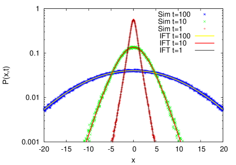
Figure 1: Probability density function $P(x,t)$ in $d=n=1$ at longer times in dimensionless form ($\sigma=\tau=D_{\star}=1$). We compare results from simulations (Sim) of the set of Langevin equations (20a) to (20c), represented by the symbols, with the direct inverse Fourier transform (IFT) of result (44). Excellent agreement is observed.

Our approach can be easily generalized to the case of the $n$-dimensional Ornstein-Uhlenbeck process considered by Jain and Sebastian klsebastian . Namely, let us consider

$$D(t)=\mathbf{Y}^{2}(t),$$ (45)

where $\mathbf{Y(t)}=\{Y_{1}(t),\ldots,Y_{n}(t)\}$ is a $n$-dimensional Ornstein-Uhlenbeck process. Since the components of $\mathbf{Y(t)}$ are independent and

$$\tau(t) = \int_{0}^{t}\mathbf{Y}^{2}(t)dt^{\prime}$$ (46)

$$= \int_{0}^{t}\left(Y_{1}^{2}(t^{\prime})+Y_{2}^{2}(t^{\prime})+\ldots+Y_{n}^{2}(t^{\prime})\right)dt^{\prime},$$

the Laplace transform $\tilde{T}_{n}(s,t)$ and the characteristic function $\hat{P}(\mathbf{k},t)$ are simply $n$-fold products of identical, one-dimensional functions (43) and (44), respectively:

$$\tilde{T}_{n}(s,t) = \exp(nt/2)\bigg{/}\Bigg{[}\frac{1}{2}\left(\sqrt{1+2s}+\frac{1}{\sqrt{1+2s}}\right)$$ (47)

$$\times\sinh\left(t\sqrt{1+2s}\right)+\cosh\left(t\sqrt{1+2s}\right)\Bigg{]}^{n/2}.$$

We thus directly obtain the exact analytical result for the Fourier transform

$$\hat{P}(\mathbf{k},t) = \exp(nt/2)\bigg{/}\Bigg{[}\frac{1}{2}\left(\sqrt{1+2k^{2}}+\frac{1}{\sqrt{1+2k^{2}}}\right)$$ (48)

$$\times\sinh\left(t\sqrt{1+2k^{2}}\right)+\cosh\left(t\sqrt{1+2k^{2}}\right)\Bigg{]}^{n/2}.$$

This result is consistent with that of Eq. (25) in Ref. klsebastian , up to numerical factors, which appear due to the difference in numerical coefficients entering the Ornstein-Uhlenbeck process.

IV.1 Brownian mean squared displacement and leptokurtic behavior

The mean squared displacement and the fourth moment encoded in our minimal model can be directly obtained from the Fourier transform (44) through differentiation,

$$\langle\mathbf{r}^{2}(t)\rangle = -\left.\nabla^{2}_{\mathbf{k}}\hat{P}(\mathbf{k},t)\right|_{\mathbf{k}=0},$$

$$\langle\mathbf{r}^{4}(t)\rangle = \left.\nabla^{4}_{\mathbf{k}}\hat{P}(\mathbf{k},t)\right|_{\mathbf{k}=0}.$$ (49)

For the isotropic case considered here the Laplace operator is defined as

$$\nabla^{2}_{\mathbf{k}}=\frac{1}{k^{d-1}}\frac{\partial}{\partial k}\left(k^{d-1}\frac{\partial}{\partial k}\right).$$ (50)

Expanding relation (41) for small $k$, we obtain up to the fourth order

$$\hat{P}(\mathbf{k},t) = \int_{0}^{\infty}e^{-k^{2}\tau}T_{n}(\tau,t)d\tau$$ (51)

$$= 1-k^{2}\int_{0}^{\infty}\tau T_{n}(\tau,t)d\tau$$

$$+\frac{k^{4}}{2}\int_{0}^{\infty}\tau^{2}T_{n}(\tau,t)d\tau+\ldots$$

From this we directly obtain the mean squared displacement

$$\langle\mathbf{r}^{2}(t)\rangle = 2d\int_{0}^{\infty}\tau T_{n}(\tau,t)d\tau=2d\langle\tau\rangle$$ (52)

$$= -2d\left.\frac{\partial\tilde{T}_{n}(s,t)}{\partial s}\right|_{s=0}$$

and the fourth order moment

$$\langle\mathbf{r}^{4}(t)\rangle = 4d(2+d)\int_{0}^{\infty}\tau^{2}T_{n}(\tau,t)d\tau=4d(2+d)\langle\tau^{2}\rangle$$ (53)

$$= 4d(d+2)\left.\frac{\partial^{2}\tilde{T}_{n}(s,t)}{\partial s^{2}}\right|_{s=0}$$

With the results of Appendix D we find

$$\langle\mathbf{r}^{2}(t)\rangle=dnt=2d\langle D\rangle_{\mathrm{st}}t,$$ (54)

where $\langle D\rangle_{\mathrm{st}}$ is given by Eq. (24), and

$$\langle\mathbf{r}^{4}(t)\rangle=4d(2+d)\langle D\rangle_{\mathrm{st}}\left[-\frac{1-e^{-2t}}{2}+t+\langle D\rangle_{\mathrm{st}}t^{2}\right].$$ (55)

Eq. (54) is the famed result of the normal Brownian, linear dispersion of the mean squared displacement with time. In dimensional units the result (54) reads

$$\langle\mathbf{r}^{2}(t)\rangle=dn\sigma^{2}\tau t=2d\langle D\rangle_{\mathrm{st}}D_{\star}t.$$ (56)

Fig. 2 demonstrates excellent agreement of the analytical result (54) with direct simulations of the set of Langevin equations (20a) to (20c) with respect to both slope and amplitude.

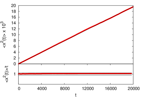
Figure 2: Mean squared displacement $\langle x^{2}(t)\rangle$ obtained from simulation of the set of Langevin equations (20a) to (20c) at $d=n=1$, corresponding to the red symbols (due to the density of points, these rather appear as the thick red line), showing excellent agreement with the Brownian law (54) shown by the (thin) full black line. In the bottom panel we show $\langle x^{2}(t)\rangle/t$, demonstrating that the deviations from the expected behavior are fairly. The grey lines (lower panel) show an interval $[0.975,1.024]$ around unity, based on $10^{6}$ trajectories.

The deviation of the shape of a distribution function from a Gaussian can be conveniently quantified in terms of the kurtosis

$$K=\frac{\langle\mathbf{r}^{4}(t)\rangle}{\langle\mathbf{r}^{2}(t)\rangle^{2}}.$$ (57)

We note that the kurtosis is closely related to the (first) non-Gaussian parameter, introduced in the classical text by Rahman rahman . Inserting results (54) and (55) we obtain in the short time limit that

$$K\sim\left(1+\frac{2}{d}\right)\left(1+\frac{1}{\langle D\rangle_{\mathrm{st}}}\right)=\left\{\begin{array}[]{ll}9,&d=1\\ 4,&d=2\\ 25/9,&d=3\end{array}\right.$$ (58)

for the choice $d=n$. At long times,

$$K\sim\left(1+\frac{2}{d}\right)=\left\{\begin{array}[]{ll}3,&d=1\\ 2,&d=2\\ 5/3,&d=3\end{array}\right..$$ (59)

The first relation characterizes exponential distributions according to Equations (66), (70), and (72) derived below, whereas the second result coincides exactly with the kurtosis of the multidimensional Gaussian distribution (note that this kurtosis does not depend on $n$). Taking along the next higher term in the long time expansion, we observe that the leptokurtosis vanishes as $\simeq 1/t$ in the long time limit,

$$K\sim 1+\frac{2}{d}+\frac{2+d}{d\langle D\rangle_{\mathrm{st}}t}.$$ (60)

In Fig. 3 we compare the analytical result (57) for the kurtosis for $d=1$ based on Equations (54) and (55) with simulations, showing excellent agreement from the short time behavior all the way to the saturation plateau at the Gaussian value $K=3$. We note that the crossover time from strongly leptokurtic to Gaussian behavior occurs at $t\approx 1$, which in dimensional units corresponds to the correlation time of the diffusing diffusivity process. Thus in experiments the behavior of the kurtosis as function of time provides a direct means to extract the correlation time of $D(t)$, which also corresponds to the crossover time from the exponential to the Gaussian behavior of the probability density $P(x,t)$, as will be shown below. We also note that when the process $\mathbf{Y}(t)$ is very highly dimensional and thus $\langle D\rangle_{\mathrm{st}}$ large, the exponential tails of $P(\mathbf{r},t)$ do not exist, see Appendix C.

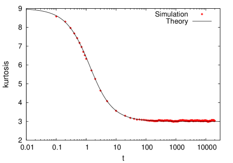
Figure 3: The Kurtosis $K$ for $d=n=1$ defined in Equation (57), based on relations (54) and (55) is shown by the full line, simulations results are represented by the symbols. The crossover occurs at the correlation time $\tau=1$. Over the entire displayed time range the agreement between theory and simulations is excellent.

We now derive explicit analytical results for the probability density function $P(\mathbf{r},t)$ in the short and long time limits, starting with the short time limit and its relation to the superstatistical formulation of the diffusing diffusivity. In our further exemplary calculations we take $n=d$. However, in Appendix C we discuss the situations when $n=1$ and $d=2$, as well as when $n$ goes to infinity while $d$ stays finite.

IV.2 Short time limit

First we concentrate on the shape of the density $P(\mathbf{r},t)$ in the short time limit $t\ll\tau$. In dimensionless units this means that we consider the asymptotic behavior of the characteristic function (48) under the condition $t\ll 1$, for which

$$\sinh\left(t\sqrt{1+2k^{2}}\right)\sim t\sqrt{1+2k^{2}},\quad\cosh\left(t\sqrt{1+2k^{2}}\right)\sim 1,$$ (61)

Together with expression (48) we thus find

$$\hat{P}(\mathbf{k},t)\sim\frac{(1+t)^{n/2}}{(1+[1+k^{2}]t)^{n/2}}\sim t^{-n/2}\left(k^{2}+\frac{1}{t}\right)^{-n/2}.$$ (62)

This expression is indeed normalized, $\hat{P}(\mathbf{k}=0,t)=1$. We can thus perform the inverse Fourier transform to obtain $P(\mathbf{r},t)$ in the short time limit.

(i) For one dimension $d=n=1$ we find

$$P(x,t)\sim\frac{1}{\pi t^{1/2}}\int_{0}^{\infty}\frac{\cos(kx)}{\left(k^{2}+1/t\right)^{1/2}}dk=\frac{1}{\pi t^{1/2}}K_{0}\left(\frac{x}{t^{1/2}}\right),$$ (63)

in terms of the Bessel function gradshteyn

$$K_{0}(a\beta)=\int_{0}^{\infty}\frac{\cos(ax)}{\sqrt{x^{2}+\beta^{2}}}dx.$$ (64)

Apart from the normalization we observe that from Eq. (63) we also derive the Brownian behavior $\langle x^{2}(t)\rangle=t=2\langle D\rangle_{\mathrm{st}}t$, in accordance with Eqs. (24) and (54).

Keeping in mind that here we are pursuing the large value limit of the scaling variable $z=xt^{-1/2}\gg 1$, we expand the Bessel function in the form abramowitz

$$K_{0}(z)\sim\sqrt{\frac{\pi}{2z}}e^{-z}.$$ (65)

We thus find the asymptotic result

$$P(x,t)\sim\frac{1}{\sqrt{2\pi|x|t^{1/2}}}\exp\left(-\frac{|x|}{t^{1/2}}\right).$$ (66)

This expression reproduces the exponential shape of the probability density function $P(x,t)$ of the diffusing diffusivity model, with the power-law correction $|x|^{-1/2}$.

Figure 4 demonstrates excellent agreement of our short time result (63) and simulations. For the longest simulated time the wings of the distribution start to show some deviations, indicating that in this case the short time limit is no longer fully justified.

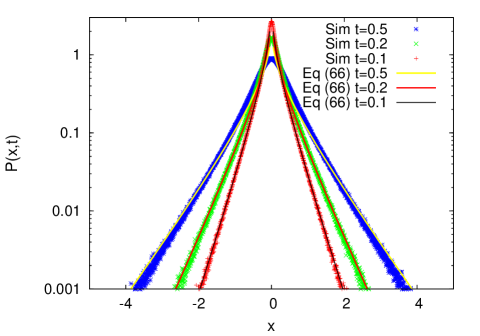
Figure 4: Probability density function $P(x,t)$ for $d=n=1$ at short times in dimensionless form ($\sigma=\tau=D_{\star}=1$). We compare results from simulations of the set of Langevin equations (20a) to (20c), represented by the symbols, with the explicit short time solution (63). Excellent agreement is observed, only for the longest time $t=0.5$ the wings start to show some deviations.

(ii) For $d=n=2$ we obtain

$$P(\mathbf{r},t) = \int e^{i\mathbf{k}\cdot\mathbf{r}}\hat{P}(\mathbf{k},t)\frac{d\mathbf{k}}{(2\pi)^{2}}$$ (67)

$$= \frac{1}{2\pi}\int_{0}^{\infty}kJ_{0}(kr)\hat{P}(k,t)dk,$$

and thus

$$P(\mathbf{r},t)=\frac{1}{2\pi t}K_{0}\left(\frac{r}{\sqrt{t}}\right).$$ (68)

Here we used the relation

$$\int_{0}^{\pi}\cos(kr\cos\varphi)d\varphi=\pi J_{0}(kr)$$ (69)

in terms of the modified Bessel function $J_{0}$. The distribution is normalized and encodes the Brownian behavior $\langle\mathbf{r}^{2}(t)\rangle=4t=4\langle D\rangle_{\mathrm{st}}t$. Expanding the Bessel function $K_{0}$ as above we find that

$$P(\mathbf{r},t)\sim\frac{1}{2\sqrt{2\pi rt^{3/2}}}e^{-r/\sqrt{t}}.$$ (70)

(iii) Finally, in $d=n=3$ the asymptotic probability density becomes

$$P(\mathbf{r},t) = \int e^{i\mathbf{k}\cdot\mathbf{r}}\hat{P}(\mathbf{k},t)\frac{d\mathbf{k}}{(2\pi)^{3}}$$ (71)

$$= \frac{1}{8\pi^{3}}\int_{0}^{\infty}k^{2}dk\int_{0}^{\pi}\sin\theta d\theta\int_{0}^{2\pi}d\varphi e^{ikr\cos\theta}$$

$$\times t^{-3/2}\left(k^{2}+\frac{1}{t}\right)^{-3/2}$$

$$= \frac{1}{4\pi^{2}t^{3/2}}\int_{0}^{\infty}k^{2}dk\int_{-1}^{1}d\xi e^{ikr\xi}\left(k^{2}+\frac{1}{t}\right)^{-3/2}$$

$$= \frac{1}{2\pi^{2}t^{3/2}}K_{0}\left(\frac{r}{\sqrt{t}}\right),$$

and we have $\langle\mathbf{r}^{2}(t)\rangle=9t=6\langle D\rangle_{\mathrm{st}}t$. Expansion of the Bessel function produces the asymptotic exponential behavior

$$P(\mathbf{r},t)\sim\frac{1}{(2\pi)^{3/2}r^{1/2}t^{5/4}}e^{-r/\sqrt{t}}.$$ (72)

As we will show in the following Subsection, in all dimensions the short time limit reproduces the superstatistical behavior. The subordination formulation, the explicit result (63) in terms of the Bessel function, and the asymptotic exponential (Laplace) form (66) (and their multidimensional analogs (68) and (70) to (72)) constitute our first main result. We note that the asymptotic forms (66), (70), and (72) of the density function $P(x,t)$ by itself leads to the Brownian scaling (54) of the corresponding mean squared displacement. When $n\neq d$ the exponential shape of the short time behavior is conserved while the subdominant prefactors change, as shown for the case $d=2$ and $n=1$ in Appendix C.

IV.3 Relation to the superstatistical approximation

Above we formulated the concept of diffusing diffusivities in terms of coupled stochastic equations for the particle position $\mathbf{r}(t)$ and the random diffusivity $D(t)$. An alternative approach suggested in Refs. granick ; gary is that of the superstatistical distribution of the diffusivity, as laid out in Section II. In this superstatistical sense the overall distribution function is given as the weighted average of a single Gaussian over the stationary diffusivity distribution,

$$P_{s}(\mathbf{r},t)=\int_{0}^{\infty}p_{D}^{\mathrm{st}}(D)G(\mathbf{r},t|D)dD.$$ (73)

(i) In dimension $d=n=1$ our minimal model produces with Eq. (28)

$$P_{s}(x,t) = \frac{1}{2\pi\sqrt{D_{\star}t}}\int_{0}^{\infty}\frac{1}{D}\exp\left(-\frac{D}{D_{\star}}-\frac{x^{2}}{4Dt}\right)dD$$ (74)

$$= \frac{1}{\pi\sqrt{D_{\star}t}}K_{0}\left(\frac{|x|}{\sqrt{D_{\star}t}}\right).$$

(ii) In $d=n=2$, we have with Eq. (32)

$$P_{s}(\mathbf{r},t) = \frac{1}{4\pi D_{\star}t}\int_{0}^{\infty}\frac{1}{D}\exp\left(-\frac{D}{D_{\star}}-\frac{r^{2}}{4Dt}\right)dD$$ (75)

$$= \frac{1}{2\pi D_{\star}t}K_{0}\left(\frac{r}{\sqrt{D_{\star}t}}\right).$$

(iii) Finally, in $d=n=3$, we find with Eq. (34)

$$P_{s}(\mathbf{r},t) = \frac{2}{\pi^{2}(4D_{\star}t)^{3/2}}\int_{0}^{\infty}\frac{1}{D}\exp\left(-\frac{D}{D_{\star}}-\frac{r^{2}}{4Dt}\right)dD$$ (76)

$$= \frac{1}{2\pi^{2}(D_{\star}t)^{3/2}}K_{0}\left(\frac{r}{\sqrt{D_{\star}t}}\right).$$

For all $d$ the mean squared displacement acquires the linear Brownian scaling in time $\langle\mathbf{r}^{2}\rangle=2d\langle D\rangle_{\mathrm{st}}t$, as it should.

This is but exactly the result of our subordination scheme in the short time limit, expressions (66), (68), and (71), written in dimensional form. Thus, in our approach to the diffusing diffusivity the short time regime of the subordination formalism leads directly to the superstatistical result. The reason is as follows: At times less than the diffusivity correlation time $\tau$ the diffusion coefficient does not change considerably, and the subordination scheme describes an ensemble of particles, each diffusing with its own diffusion coefficient. This mimics a spatially inhomogeneous situation, when the local diffusion coefficient is random, but stays constant within confined spatial domains. In this case the ensemble of particles moving in different domains exhibits a superstatistical behavior, as assumed in the original works beck . However, in any system with finite patch sizes, we would not expect the particles to stay in their local patch of diffusivity $D$ forever, thus violating the assumption of the superstatistical approach. Our annealed approach in some sense delivers a mean field approximation to the spatially disordered situation, and adequately describes the transition from short time superstatistical behavior to the Gaussian probability law at long times, which will be shown in the subsequent section. The full consistency in the short time limit between the subordination approach and superstatistics is our second main result.

IV.4 Long time limit

We now turn to the long time limit encoded in the Fourier transform (44) of the probability density $P(\mathbf{r},t)$, that is, the times larger than the diffusivity correlation time $\tau$. In dimensionless units it corresponds to $t\gg 1$, and the hyperbolic functions assume the limiting behaviors

$$\sinh\left(t\sqrt{1+2k^{2}}\right) \sim \cosh\left(t\sqrt{1+2k^{2}}\right)$$ (77)

$$\sim \frac{1}{2}\exp\left(t\sqrt{1+2k^{2}}\right).$$

Combined with result (48) we find

$$\hat{P}(\mathbf{k},t)\sim\frac{2^{n/2}\exp\left(\frac{nt}{2}\left[1-\sqrt{1+2k^{2}}\right]\right)}{\left(1+\frac{1}{2}\left[\sqrt{1+2k^{2}}+\frac{1}{\sqrt{1+2k^{2}}}\right]\right)^{n/2}}.$$ (78)

As in the short time limit above, this expression is normalized, $\hat{P}(\mathbf{k}=0,t)=1$.

Now let us focus on the tails of the probability density $P(\mathbf{r},t)$, corresponding to the limit $k\ll 1$, for which Eq. (78) gives $\hat{P}(\mathbf{k},t)\sim\exp(-nk^{2}t/2)=\exp\left(-\langle D\rangle_{\mathrm{st}}k^{2}t\right)$, and thus

$$P(\mathbf{r},t)\sim\frac{1}{(4\pi\langle D\rangle_{\mathrm{st}}t)^{n/2}}\exp\left(-\frac{\mathbf{r}^{2}}{4\langle D\rangle_{\mathrm{st}}t}\right).$$ (79)

At long times the probability density function $P(\mathbf{r},t)$ assumes a Gaussian form, with the effective diffusivity $\langle D\rangle_{\mathrm{st}}=n/2$. This is a consequent result given the Ornstein-Uhlenbeck variation of the diffusivity encoded in the starting equations (19b) and (19c): at sufficiently long times the process samples the full diffusivity space and behaves like an effective Gaussian process with renormalized diffusivity. The explicit derivation of the crossover to the Gaussian behavior is our third main result.

Fig. 5 shows the crossover from the initial exponential to the long time Gaussian behavior of the probability density function $P(x,t)$ for $d=n=1$ by comparison to the Gaussian distribution (79) for short time $t=0.1$, the crossover time $t=1.0$ and the longer time $t=10.0$.

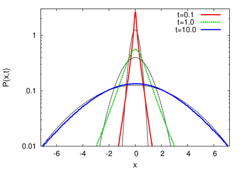
Figure 5: Probability density function $P(x,t)$ for $d=n=1$ from simulations of the Langevin equations (20) for three different times, in dimensionless form ($\sigma=\tau=D_{\star}=1$). Comparison with Gaussian distribution (79) demonstrates the strongly non-Gaussian behavior at short times and the almost fully Gaussian shape at longer times.

V Bivariate Fokker-Planck equation and relation to the subordination approach

In this section we derive the Fokker-Planck equation corresponding to the set of stochastic equations (20a) to (20c) of our diffusing diffusivity model. We will also establish the relation to the subordination approach of section IV. Note that we here restrict the discussion to the case $d=n=1$, as higher dimensional cases are completely equivalent.

Following our notation we thus seek the Fokker-Planck equation for the bivariate probability density function $f(x,y,t)$, which has the structure

$$\frac{\partial}{\partial t}f(x,y,t)=\mathscr{L}_{y}f(x,y,t)+y^{2}\frac{\partial^{2}}{\partial x^{2}}f(x,y,t).$$ (80)

The Fokker-Planck operator in $y$ reads

$$\mathscr{L}_{y}=\frac{\partial}{\partial y}y+\frac{1}{2}\frac{\partial^{2}}{\partial y^{2}},$$ (81)

and the marginal probability density function for $x$ is then

$$P(x,t)=\int_{-\infty}^{\infty}f(x,y,t)dy.$$ (82)

To proceed further we introduce the joint probability density function $q(\tau,y,t)$ of the Ornstein-Uhlenbeck process $y(t)$ and its integrated square $\tau(t)$, given by equation (39). The corresponding system of stochastic equations has the form

$$\frac{dy}{dt} = -y+\eta(t),$$ (83a)

$$\frac{d\tau}{dt} = y^{2},$$ (83b)

and thus the bivariate Fokker-Planck equation governing the probability density $q(\tau,y,t)$ reads

$$\frac{\partial}{\partial t}q(\tau,y,t)=\mathscr{L}_{y}q(\tau,y,t)-y^{2}\frac{\partial}{\partial\tau}q(\tau,y,t).$$ (84)

Now we introduce an ansatz for the solution of equation (80) of the form

$$f(x,y,t)=\int_{0}^{\infty}G(x,\tau)q(\tau,y,t)d\tau,$$ (85)

where $G(x,\tau)$ is the Gaussian probability density given by equation (37). Then, in accordance with equation (82) the marginal probability density $P(x,t)$ can be written in the subordination form of equation (38), where

$$T(\tau,t)=\int_{\infty}^{\infty}q(\tau,y,t)dy$$ (86)

is the marginal probability density function of the integrated square of the Ornstein-Uhlenbeck process whose Laplace transform is given by equation (42).

We now prove that the solution of equation (80) can be presented in the form (85). To that end we differentiate equation (85) and use relation (84) to get

$$\frac{\partial}{\partial t}f(x,y,t) = \int_{0}^{\infty}G(x,\tau)\frac{\partial}{\partial t}q(\tau,y,t)d\tau$$ (87)

$$=\int_{0}^{\infty}G(x,\tau)\left[\mathscr{L}_{y}q(x,y,t)-y^{2}\frac{\partial}{\partial\tau}q(x,y,t)\right]d\tau$$

$$=\mathscr{L}_{y}\left[\int_{0}^{\infty}G(x,\tau)q(\tau,y,t)d\tau\right]$$

$$-y^{2}\int_{0}^{\infty}G(x,\tau)\frac{\partial}{\partial\tau}q(x,y,t)d\tau.$$

We now apply relation (85) to the first term and integrate the second term by parts, obtaining

$$\frac{\partial}{\partial t}f(x,y,t) = \mathscr{L}_{y}f(x,y,t)-y^{2}\left\{q(\tau,y,t)G(x,\tau)\Big{|}^{\tau=\infty}_{\tau=0}\right.$$ (88)

$$-\left.\int_{0}^{\infty}q(\tau,y,t)\frac{\partial}{\partial\tau}G(x,\tau)d\tau\right\}.$$

Finally, with the relation $\partial G(x,\tau)/\partial\tau=\partial^{2}G(x,\tau)/\partial x^{2}$, we see that

$$\frac{\partial}{\partial t}f(x,y,t) = \mathscr{L}_{y}f(x,y,t)+y^{2}\frac{\partial^{2}}{\partial x^{2}}f(x,y,t)$$ (89)

$$+y^{2}q(\tau=0,y,t)\delta(x).$$

The last term vanishes, as $\tau$ is the integrated square of $y(t)$, and thus we arrive at equation (80). Therefore we showed that the solution of the bivariate Fokker-Planck equation (80) can be presented in the form (85), and consequently the marginal probability density function $P(x,t)$ can be written in the subordination form (38).

The connection of the bivariate Fokker-Planck equation (80) for the Langevin system (19a) to (19c) with the subordination approach represented by relations (36) and (38) is our fourth main result.

VI Discussion

An increasing number of systems are reported in which the mean squared displacement is linear in time, suggesting normal (Fickian) diffusion of the observed tracer particles. Concurrently the (displacement) probability density function is pronouncedly non-Gaussian. Normal diffusion with a Laplace distribution of particle displacements was previously explained in a superstatistical approach by Granick and coworkers granick . The experimentally observed crossover to Gaussian statistics at longer times was interpreted as a consequence of the central limit theorem, kicking in at times longer then the correlation time of the diffusion fluctuations granick . Chubinsky and Slater gary introduced the diffusing diffusivity model and studied it numerically, concluding the crossover from the initial exponential shape to a Gaussian with effective diffusivity. Jain and Sebastian go further with the double Langevin approach klsebastian . Here we introduced a consistent minimal model for a diffusing diffusivity. We explicitly obtain the Fourier transform of the full probability density function, from which we derive the analytical short and long time limits. This allows us to determine the dynamical crossover to the long time Gaussian shape of the probability density at the correlation time of the fluctuating diffusivity. Moreover we demonstrate a full consistency of our minimal model with the superstatistical approach, as well as with the results of Jain and Sebastian. At the same time our model is more general and flexible: phrasing the diffusing diffusivity approach in terms of a subordination concept we endow our model with an extremely flexible basis, such that a wide range of different statistics for the diffusivity can be included.

We also obtained the bivariate Fokker-Planck equation for this diffusing diffusivity process and expressed its solution in terms of the subordination integral. Excellent agreement with simulations is provided for the probability density function, the Brownian scaling of the mean squared displacement, and the kurtosis of the probability density function.

We are confident that this subordination integral formulation of the diffusing diffusivity model will prove useful for experimentalists observing such dynamics. The model can be calibrated with respect to the two parameters $\tau$ and $\sigma$, which can be obtained from experiment by analyzing the time-dependence of the mean squared displacement and the kurtosis. The latter provides information on the typical diffusivity correlation time $\tau$ (see Fig. 3), whereas the former allows one to estimate the parameter $\sigma$, see Eq. (56). Moreover, measurement of the diffusivity distribution, as can be directly obtained experimentally spako , provides the value of the parameter $D_{\star}=\sigma^{2}\tau$ according to Eq. 28. Additionally, the possibility to include a different dimensionality $n$ for the subordinating process $\mathbf{Y}(t)$ allows for fine-tuning of the model to match the experimentally observed probability density function, which might be necessary when the model is used for quantitative predictions. As we show in the example in Appendix C1 the difference in the dimensionality $n$ of the process $\mathbf{Y}(t)$ does not change the dominant exponential behavior at short times but affects the prefactors. Similarly the prefactors of the exponential in the diffusivity distribution $p_{D}^{\mathrm{st}}(D)$ is affected by the concrete value of $n$. This fact may be employed to account for the deviations from the pure exponential shape of the probability distribution also reported in granick .

An intriguing question emerging from our analysis concerns the physical origin of the dimensionality $n$ of the subordinating process $\mathbf{Y}(t)$. Intuitively, one might argue that the diffusivity and thus $\mathbf{Y}(t)$ should have as many components as spatial directions in the particle trajectory $\mathbf{r}(t)$, i.e., $d=n$. This is the case considered in the derivations in Section IV. However, the mode concept for $D(t)$ introduced here may also have a more fundamental physical meaning. As we showed here, the value $n$ affects the details of the shape of $P(\mathbf{r},t)$ as well as $p_{D}^{\mathrm{st}}(D)$, and for large $n$ values the short time exponential shapes may even be fully suppressed. Advanced experiments allowing one to determine $n$ from the exact shape of the probability densities $P(\mathbf{r},t)$ and $p_{D}^{\mathrm{st}}(D)$ will provide important clues concerning this question.

Possible generalizations may include diffusing diffusivity models with additional deterministic time dependence of the diffusivity sbmdiff1 or non-Gaussian anomalous viscoelastic diffusion in crowded membranes membranesa , which contrasts Gaussian anomalous viscoelastic diffusion in non-crowded membranes membranesc . Of course, the diffusing diffusivity concept is a first step in capturing the full spatiotemporal disorder of complex systems. Ultimately, a full description of spatial and temporal stochasticity in terms of a random diffusivity $D(x,t)$ will be desired.

Let us put the diffusing diffusivity approach into context with other popular models with distributed transport coefficients. Typically these are constructed to describe anomalous diffusion processes. Another model is scaled Brownian motion, in which the diffusivity is a deterministic, power-law function of time lim ; fulinski . On a stochastic level scaled Brownian motion appears naturally in granular gases gasbook , in which non-ideal collisions effect a decrease of the system’s temperature (kinetic energy). Scaled Brownian motion is non-ergodic and displays a massively delayed overdamping transition sbm . Heterogeneous diffusion processes employ a continuous, deterministic space dependence of the diffusivity and lead to non-ergodic and ageing dynamics hdp ; hdpa ; fulinski . In contrast to these models random diffusivity approaches also have a considerable history. Thus segregation in solids in the context of radiation was described by such an approach dubinko , and Brownian motion in media with fluctuating friction coefficient, temperature fluctuations, or randomly interrupted diffusion were used to describe, for instance, randomly stratified media luczka-talkner . A random diffusivity approach was elaborated to consider light scattering in a continuous medium with fluctuating dielectric constant kravtsov . Motivated by the comparison of diffusion processes assessed by different modern measurement techniques, the concept of microscopic single-particle diffusivity was developed radons . In lapeyre the diffusivity varies randomly but is constant on patches of random sizes. Such random patch model show non-ergodic subdiffusion due to the diffusivity effectively changing at random times with a heavy-tailed distribution. Intermittency between two values of the diffusivity were also considered sbmdiff . Finally, we mention that a deterministic time dependence of the diffusivity was combined with a random diffusivity in sbmdiff1 . As seen in several experimental studies already, to describe stochastic particle motion in real complex systems such as living biological cells, combinations of different stochastic mechanisms are necessary to capture the observed dynamics goldinga . Thus also the diffusing diffusivity picture may need to be complemented by other processes, as we saw in the example of non-Gaussian viscoelastic subdiffusion based on the observations in spako ; membranesa .

Despite the wealth of established stochastic processes the diffusing diffusivity model has quite unique properties. Thus the crossover from a short time exponential shape to Gaussian statistics at longer times, while the MSD remains linear and thus classifies normal (Fickian) diffusion, cannot be captured by existing models. Of course, crossovers between non-Gaussian to Gaussian probability density functions may be grasped by truncated continuous time random walks or distributed order fractional diffusion equations truncate . However, in these models also the MSD exhibits a crossover from anomalous to normal diffusion. In this sense we believe that the diffusing diffusivity model and its potential generalizations on the basis of our subordination approach will emerge as a new paradigm in the theory of stochastic processes.

We conclude with pointing out that the diffusing diffusivity model developed here is closely related to the Cox-Ingersoll-Ross (CIR) model for monetary returns which is widely used in financial mathematics cir . To show this relation let us write the Langevin equation (19c) for the Ornstein-Uhlenbeck process as

$$dY_{i}=-\frac{1}{\tau}Y_{i}dt+\sigma dW_{i}(t),$$ (90)

where $i=1,\ldots,n$ and $W_{i}(t)$ is the Wiener process with variance $1/2$. Our aim is to design a Langevin equation in the Itô form for the squared Ornstein-Uhlenbeck process in $n$ dimensions,

$$D(t)=\sum_{i=1}^{n}Y_{i}^{2}(t).$$ (91)

To this end we employ the Itô formula of differentiation to the function of a $n$-dimensional vector gardiner to find

$$dD=\frac{2}{\tau}\left(\frac{n\sigma^{2}\tau}{2}-D\right)+2\sigma\sqrt{D}dW(t).$$ (92)

This is but the stochastic differential equation of the CIR process describing the time evolution of interest rates cir . The same process is used in the Heston model specifying the evolution of stochastic volatility of a given asset heston . Our results for the subordination approach should therefore also be relevant to financial market modeling. Indeed, the technique of subordination, which is closely related to random time changes, is a very common concept in financial mathematics clark .

Appendix A Superstatistics with modified exponential diffusivity distribution

Consider the Gaussian probability density function typical for viscoelastic subdiffusion in the overdamped limit,

$$G_{\alpha}(x,t|D_{\alpha})=\frac{1}{\sqrt{4\pi D_{\alpha}t^{\alpha}}}\exp\left(-\frac{x^{2}}{4D_{\alpha}t^{\alpha}}\right),$$ (93)

which is equivalent to fractional Brownian motion pccp . The associated mean squared displacement is $\langle x^{2}(t)\rangle=2D_{\alpha}t^{\alpha}$. For the superstatistical distribution of the generalized diffusion coefficient we choose the modified exponential

$$p_{D}(D_{\alpha})=\frac{1}{\Gamma(1+1/\kappa)D_{\alpha}^{\star}}\exp\left(-\left[\frac{D_{\alpha}}{D_{\alpha}^{\star}}\right]^{\kappa}\right).$$ (94)

Figure 6: Top: Superstatistical probability density function $P_{s}(x,t)$ according to Equation (95) from numerical integration, for exponents $\kappa=0.5$, $1$, and $2$ (see the Figure key). Bottom: convergence of the full numerical solution to the analytical asymptotic form (102) for $\kappa=0.5$ and $2$. All distributions are drawn for $t=1$ (a.u.).

The resulting probability density function

$$P_{s}(x,t)=\int_{0}^{\infty}p_{D}(D_{\alpha})G_{\alpha}(x,t|D_{\alpha})dD_{\alpha}$$ (95)

with $D_{\alpha}/D_{\alpha}^{\star}\to\tilde{D}$ and $\lambda=x^{2}/[4D_{\alpha}^{\star}t^{\alpha}]$ becomes

$$P_{s}(x,t)=\frac{1}{\sqrt{4\pi D_{\alpha}^{\star}t^{\alpha}}\Gamma(1+1/\kappa)}\int_{0}^{\infty}\tilde{D}^{-1/2}e^{-\tilde{D}^{\kappa}-\lambda/\tilde{D}}d\tilde{D}.$$ (96)

After change of variables according to $y=\tilde{D}^{\kappa}$ we have

$$P_{s}(x,t) = \frac{1}{\sqrt{4\pi D_{\alpha}^{\star}t^{\alpha}}\kappa\Gamma(1+1/\kappa)}$$ (97)

$$\times\int_{0}^{\infty}y^{-1+1/(2\kappa)}e^{-y-\lambda y^{-1/\kappa}}dy.$$

With the identification

$$e^{-z}=H^{1,0}_{0,1}\left[z\left|\begin{array}[]{l}\rule{39.83368pt}{0.56917pt}\\ (0,1)\end{array}\right.\right]$$ (98)

with the Fox $H$-function mathai , using the Laplace transform rules for the $H$-function wgg along with the standard rules for the Fox $H$-function mathai one arrives at the result

$$P_{s}(x,t) = \frac{1}{\Gamma(1/\kappa)\sqrt{4\pi D_{\alpha}^{\star}t^{\alpha}}}$$ (101)

$$\times H^{2,0}_{0,2}\left[\frac{x^{2}}{4D_{\alpha}^{\star}t^{\alpha}}\left|\begin{array}[]{l}\rule{39.83368pt}{0.56917pt}\\ (1/[2\kappa],1/\kappa),(0,1)\end{array}\right.\right].$$

The asymptotic behavior is then mathai

$$P_{s}(x,t) \simeq \frac{|x|^{(1-\kappa)/(1+\kappa)}}{\Gamma(1/\kappa)\sqrt{\pi}(4D_{\alpha}^{\star}t^{\alpha})^{1/(1+\kappa)}}$$ (102)

$$\times\exp\left(-\frac{1+\kappa}{\kappa^{\kappa/(1+\kappa)}}\left[\frac{x^{2}}{4D_{\alpha}^{\star}t^{\alpha}}\right]^{\kappa/(1+\kappa)}\right).$$

In Figure 6 we show the behavior of the resulting probability density (95) from numerical inversion. For compressed exponential distributions $p_{D}(D_{\alpha})$ with $\kappa>1$ the resulting function $P_{s}(x,t)$ is a stretched Gaussian, while for a stretched exponential $p_{D}(D_{\alpha})$ with $0<\kappa<1$ the function $P_{s}(x,t)$ is a superstretched Gaussian, which is broader than the exponential (Laplace) distribution. Figure 6 also demonstrates that the asymptotic behavior (102) indeed fits the numerical inversion.

Asymptotics by Laplace’s method

The asymptotic behavior (102) may also be obtained by the Laplace method. As this is an interesting alternative method to derive the asymptotic behavior of the integral (see Eq. (96))

$$I=\int_{0}^{\infty}\tilde{D}^{-1/2}e^{-\tilde{D}^{\kappa}-\lambda/\tilde{D}}d\tilde{D}=\int_{0}^{\infty}y^{-3/2}e^{-y^{-\kappa}-\lambda y}dy$$ (103)

for $\lambda\gg 1$, we include this approach here. This is a Laplace integral of the form

$$I=\int_{0}^{\infty}f(y)e^{-\lambda y}dy.$$ (104)

The standard methods to evaluate the asymptotics of $I$ cannot be applied, since $f(y)$ in Eq. (103) equals zero at $y=0$ with all its derivatives. Thus, to evaluate the asymptotics we need to find the maximum of the function

$$\varphi(y)=-\lambda y-y^{-\kappa}$$ (105)

which is reached at $y_{m}=(\kappa/\lambda)^{1/(1+\kappa)}$. We now introduce the new variable $t=y/y_{m}$, such that Eq. (103) becomes

$$I = \left(\frac{\lambda}{\kappa}\right)^{1/[2(1+\kappa)]}\int_{0}^{\infty}t^{-3/2}\exp\left(-\lambda^{\kappa/(1+\kappa)}\right.$$ (106)

$$\left.\times\left[\kappa^{-\kappa/(1+\kappa)}t^{-\kappa}+t\kappa^{1/(1+\kappa)}\right]\right).$$

After substitution $\tau=t\kappa^{1/(1+\kappa)}$ we get

$$I=\lambda^{1/[2(1+\kappa)]}\int_{0}^{\infty}\tau^{-3/2}e^{\overline{\lambda}S(\tau)}d\tau,$$ (107)

where $\overline{\lambda}=\lambda^{\kappa/(1+\kappa)}$ and $S(\tau)=-\tau-\tau^{-\kappa}$.

Now, the standard Laplace method can be applied to Eq. (107). The function $S(\tau)$ reaches its maximum at $\tau_{m}=\kappa^{1/(1+\kappa)}$. Following the standard procedure we find

$$I \sim \lambda^{1/[2(1+\kappa)]}\int_{\tau_{m}-\varepsilon}^{\tau_{m}+\varepsilon}\tau^{-3/2}$$ (108)

$$\times\exp\left(\overline{\lambda}\left[S(\tau_{m})+\frac{(\tau-\tau_{m})^{2}}{2}S^{\prime\prime}(\tau_{m})\right]\right)$$

$$\sim \lambda^{1/[2(1+\kappa)]}\tau_{m}^{-3/2}e^{\overline{\lambda}S(\tau_{m})}\int_{\infty}^{\infty}\exp\left(-\frac{\overline{\lambda}}{2}\left|S^{\prime\prime}(\tau_{m})\right|\tau^{2}\right)$$

$$= \lambda^{1/[2(1+\kappa)]}\tau_{m}^{-3/2}e^{\overline{\lambda}S(\tau_{m})}\sqrt{\frac{2\pi}{\overline{\lambda}S^{\prime\prime}(\tau_{m})}}.$$

With $S(\tau_{m})=-(1+\kappa)\kappa^{-\kappa/(1+\kappa)}$ and $S^{\prime\prime}(\tau_{m})=-(1+\kappa)\kappa^{-1/(1+\kappa)}$ and applying this result to the above probability density function (96), we obtain the same asymptotic behavior (102), up to a numerical prefactor.

Power law diffusivity distribution

We now consider the power law distribution

$$p_{D}(D)=\frac{\alpha D_{\star}^{\alpha}}{(D_{\star}+D)^{1+\alpha}}$$ (109)

with $\alpha>0$. With the relation (7) we separately consider the following cases:

(i) $0<\alpha<1$. The Laplace transform of the diffusivity distribution reads

$$\tilde{p}_{D}(s) = \alpha D_{\star}^{\alpha}\int_{0}^{\infty}\frac{dD}{(D_{\star}+D)^{1+\alpha}}e^{-Ds}dD$$ (110)

$$=1-D_{\star}s^{\alpha}e^{D_{\star}s}\left(\Gamma(1-\alpha)-\int_{0}^{D_{\star}s}z^{-\alpha}e^{-z}dz\right),$$

after substituting and integrating by parts. In the tails we then obtain the following scaling behavior for the probability density function,

$$\lim_{k\to 0}P(k,t) \sim 1-D_{\star}k^{2\alpha}t^{\alpha}\left(1+D_{\star}k^{2}t+\ldots\right)$$ (111)

$$\times\left[\Gamma(1-\alpha)-\frac{(D_{\star}k^{2}t)^{1-\alpha}}{1-\alpha}+\frac{(D_{\star}k^{2}t)^{2-\alpha}}{2-\alpha}-\ldots\right].$$

It thus follows that

$$P(x,t)\simeq\frac{1}{|x|^{2\alpha+1}}$$ (112)

such that the second moment does not exist.

(ii) $\alpha=1$. After integrating by parts once we obtain

$$P(k,t)\sim 1-D_{\star}k^{2}t\log(D_{\star}k^{2}t).$$ (113)

The second moment still does not exist.

(iii) $1<\alpha<2$. Integrating by parts twice, we find

$$\tilde{p}_{D}(s) = 1-\frac{D_{\star}s}{\alpha-1}+\frac{D_{\star}^{\alpha}s^{\alpha}e^{D_{\star}s}}{\alpha-1}$$ (114)

$$\times\left(\Gamma(2-\alpha)-\int_{0}^{D_{\star}s}z^{1-\alpha}e^{-z}dz\right),$$

such that we obtain

$$P(x,t)\simeq\frac{1}{|x|^{2\alpha+1}}$$ (115)

with the MSD

$$\langle x^{2}(t)\rangle\sim\frac{2D_{\star}}{\alpha-1}t.$$ (116)

Power law diffusivity distributions lead to a long tailed, power law distribution $P(x,t)$ in the superstatistical approach. The second moment diverges for $0<\alpha\leq 1$, while normal diffusion emerges for $\alpha>1$.

Appendix B Dimensionless units for the minimal model

To simplify the calculations and obtain a more elegant formulation we introduce dimensionless variables according to $t^{\prime}=t/t_{0}$ and $x^{\prime}=x/x_{0}$ (and similarly for the $y$ and $z$ components). For the $x$ component, the set (19) of stochastic equations then becomes

$$\frac{d}{dt^{\prime}}x^{\prime}(t) = \frac{t_{0}}{x_{0}}\sqrt{2D(t)}\xi(t_{0}t^{\prime})$$ (117a)

$$D(t) = Y^{2}(t)$$ (117b)

$$\frac{d}{dt^{\prime}}Y = -\frac{Y}{\tau/t_{0}}+\sigma\eta(t_{0}t^{\prime}).$$ (117c)

Noting that for the Gaussian noise sources we have $\xi(t_{0}t^{\prime})=t_{0}^{-1/2}\xi(t^{\prime})$ and $\eta(t_{0}t^{\prime})=t_{0}^{-1/2}\eta(t^{\prime})$ we rewrite Eqs. (117) as

$$\frac{d}{dt^{\prime}}x^{\prime}(t) = \sqrt{2\overline{D}(t)}\xi(t^{\prime})$$ (118a)

$$\overline{D}(t) = \overline{Y}^{2}(t)$$ (118b)

$$\frac{d}{dt^{\prime}}\overline{Y} = -\frac{\overline{Y}}{\overline{\tau}}+\overline{\sigma}\eta(t^{\prime}),$$ (118c)

where

$$\overline{D}=\frac{t_{0}}{x_{0}^{2}}D,\quad\overline{Y}=\frac{t_{0}^{1/2}}{x_{0}}Y,\quad\overline{\tau}=\frac{\tau}{t_{0}}.$$ (119)

Now we choose the temporal and spatial scales such that $\overline{\tau}=\overline{\sigma}=1$, that is,

$$t_{0}=\tau,\quad x_{0}=\sigma\tau.$$ (120)

With this choice of units the stochastic equations of our minimal diffusing diffusivity model are then given by Eqs. (20).

Appendix C Two examples for the process $\mathbf{Y}(t)$

C.1 The case $d=2$ and $n=1$

As an example for the case when the dimensionality of the process $\mathbf{Y}(t)$ differs from the embedding dimension $d$ of the process $\mathbf{r}(t)$ we take the case with $d=2$ and $n=1$. In the short time limit we get from Eq. (62) that

$$P(\mathbf{r},t) \sim \frac{1}{2\pi t^{1/2}}\int_{0}^{\infty}\frac{kJ_{0}(kr)}{\sqrt{k^{2}+1/t}}dk$$ (121)

$$= \frac{1}{\sqrt{2\pi^{3}}t}\left(\frac{r}{\sqrt{t}}\right)^{-1/2}K_{1/2}\left(\frac{r}{\sqrt{t}}\right).$$

The asymptotic behavior is given by

$$P(\mathbf{r},t)\sim\frac{1}{2\pi r\sqrt{t}}e^{-t/\sqrt{t}}.$$ (122)

Comparing this result with Eq. (70) for the case $d=n=2$ we recognize the modified prefactor, including a different scaling in $r$ and $t$. Thus the difference in the dimensionality of the process $\mathbf{Y}(t)$ does not change the dominating exponential behavior.

The connection to the superstatistical approach in analogy to the discussion in Section IV.3 following Eq. (73) with the two-dimensional Gaussian kernel

$$G(\mathbf{r},t|D)=\frac{1}{4\pi Dt}e^{-r^{2}/(4Dt)}$$ (123)

and the stationary diffusivity distribution

$$p_{D}^{\mathrm{st}}(D)=\frac{1}{\sqrt{\pi DD_{\star}}}e^{-D/D_{\star}}$$ (124)

for the case $n=1$ produces the distribution

$$P(\mathbf{r},t)=\frac{1}{\sqrt{2\pi^{3}}D_{\star}t}\left(\frac{r}{\sqrt{D_{\star}t}}\right)^{-1/2}K_{1/2}\left(\frac{r}{\sqrt{D_{\star}t}}\right).$$ (125)

which matches exactly Eq. (121) written in dimensional form.

C.2 Infinite-dimensional process $\mathbf{Y}(t)$

We here consider the limit of large dimension $n$ for the process $\mathbf{Y}(t)$. For short times $t\ll 1$ the tails of the probability density $P(\mathbf{r},t)$ follow from (compare Eq. (48))

$$\hat{P}(\mathbf{k},t) \sim \frac{e^{nt/2}}{\left[\frac{t}{2}\left(1+2k^{2}+1\right)+1\right]^{n/2}}$$ (126)

$$= \frac{e^{nt/2}}{\left[1+\frac{t(1+k^{2})\frac{n}{2}}{n/2}\right]^{n/2}}$$

$$\to \frac{e^{nt/2}}{e^{(1+k^{2})nt/2}}=e^{-ntk^{2}/2}.$$

Thus the tails of the probability density function $P(x,t)$ are Gaussian already at short times.

The long time behavior $t\gg 1$ leads to

$$\hat{P}(\mathbf{k},t)\sim\frac{2^{n/2}\exp\left(\frac{nt}{2}\left[1-\sqrt{1+2k^{2}}\right]\right)}{\left[1+\frac{1}{2}\left(\sqrt{1+2k^{2}}+\frac{1}{\sqrt{1+2k^{2}}}\right)\right]^{n/2}}.$$ (127)

Considering the tails, we take $k\ll 1$, revealing that

$$\hat{P}(\mathbf{k},t)\sim\exp\left(-\frac{nk^{2}t}{2}\right)$$ (128)

is also Gaussian, with the same variance. Thus, in the high-dimensional case the regime of exponential wings in the probability density function does not exist at all and the Gaussian shape is established early on. This is equivalent to the observation that the kurtosis (57) becomes Gaussian already for short times when $n$ is large.

Appendix D Fourth moment of $P(x,t)$

By help of relation (41) we obtain the fourth moment of $P(x,t)$. The necessary derivative of $\tilde{T}_{n}(s,t)$ with respect to $s$ is

$$\frac{\partial\tilde{T_{n}}(s,t)}{\partial s} = -\frac{ne^{nt/2}}{2}\left[\frac{1}{2}\left(\sqrt{1+2s}+\frac{1}{\sqrt{1+2s}}\right)\sinh\left(t\sqrt{1+2s}\right)+\cosh\left(t\sqrt{1+2s}\right)\right]^{-n/2-1}\left[\frac{s}{(1+2s)^{3/2}}\sinh\left(t\sqrt{1+2s}\right)\right.$$ (129)

$$+\frac{t}{2}\left(1+\frac{1}{1+2s}\right)\cosh\left(t\sqrt{1+2s}+\frac{t}{\sqrt{1+2s}}\sinh\left(t\sqrt{1+2s}\right)\right],$$

and thus

$$\left.\frac{\partial\tilde{T}_{n}(s,t)}{\partial s}\right|_{s=0}=-\frac{nt}{2}.$$ (130)

The second differentiation and subsequent limit $s\to 0$ produces, after some steps,

$$\frac{\partial^{2}\tilde{T_{n}}(s,t)}{\partial s^{2}}\Big{|}_{s=0}=\left<\tau^{2}(t)\right>=-\frac{n}{4}\left(1-e^{-2t}\right)+\frac{nt}{2}+\frac{n^{2}t^{2}}{4}.$$ (131)