Microscopic Mechanism and Kinetics of Ice Formation at Complex Interfaces: Zooming in on Kaolinite

Abstract

Most ice in nature forms thanks to impurities which boost the exceedingly low nucleation rate of pure supercooled water. However, the microscopic details of ice nucleation on these substances remain largely unknown. Here, we have unraveled the molecular mechanism and the kinetics of ice formation on kaolinite, a clay mineral playing a key role in climate science. We find that the formation of ice at strong supercooling in the presence of this clay is twenty orders of magnitude faster than homogeneous freezing. The critical nucleus is substantially smaller than that found for homogeneous nucleation and, in contrast to the predictions of classical nucleation theory (CNT), it has a strong 2D character. Nonetheless, we show that CNT describes correctly the formation of ice at this complex interface. Kaolinite also promotes the exclusive nucleation of hexagonal ice, as opposed to homogeneous freezing where a mixture of cubic and hexagonal polytypes is observed.

The formation of ice is at the heart of intracellular freezing Tam et al. (2009), stratospheric ozone chemistry Bolton and Pettersson (2001), cloud dynamics Tang, Cziczo, and Grassian (2016), rock weathering Bartels-Rausch et al. (2012) and hydrate formation Pirzadeh and Kusalik (2013). As ice nucleation within pure supercooled liquid water is amazingly rare in nature, most of the ice on Earth forms heterogeneously, in the presence of foreign particles which boost the ice nucleation rate Murray et al. (2012). These substances, which can be as diverse as soot Lupi, Hudait, and Molinero (2014), bacterial fragments O’Sullivan et al. (2015) or mineral dust Eastwood et al. (2008), lower the free energy barrier for nucleation and make ice formation possible even at a few degrees of supercooling. However, the microscopic details of heterogeneous ice nucleation are still poorly understood. State-of-the-art experimental techniques can establish whether a certain material is efficient in promoting heterogeneous ice nucleation, but it is very challenging to achieve the temporal and spatial resolution required to characterize the process at the molecular level. On the other hand, spontaneous fluctuations that produce nuclei of critical size are rare events. They thus happen on timescales (seconds) that are far beyond the reach of classical molecular dynamics simulations. This is why, to our knowledge, quantitative simulations of heterogeneous ice nucleation have been successful only when using the coarse grained mW model for water Lupi, Hudait, and Molinero (2014); Fitzner et al. (2015); Cabriolu and Li (2015). Such simulations have gone a long way towards improving our fundamental understanding of heterogeneous ice nucleation, but coarse grained models are not appropriate for many of the more complex and interesting ice nucleating substrates.

A representative example is the formation of ice on clay minerals - a phenomenon critical to cloud formation and dynamics Zimmermann et al. (2008); Eastwood et al. (2008). For instance, the heterogeneous ice nucleation probability in the presence of kaolinite, a clay mineral well studied by both experiments Murray et al. (2011, 2012); Tobo et al. (2012); Welti et al. (2013); Wex et al. (2014) and simulations Hu and Michaelides (2010); Tunega, Gerzabek, and Lischka (2004); Cox et al. (2014); Zielke et al. (2016), seems to be related to its surface area Murray et al. (2011), but how exactly this material facilitates the formation of the ice nuclei is largely unestablished. Classical molecular dynamics simulations have recently succeeded in simulating ice nucleation on kaolinite Cox et al. (2014); Zielke et al. (2016). However, finite size effects Cox et al. (2014) and rigid models of the surface Zielke et al. (2016) prevented the extraction of quantitative results. In fact, it is exceedingly challenging to compute via atomistic simulations ice nucleation rates, which have been inferred (for homogeneous freezing only) along a wide range of temperatures Sanz et al. (2013) and recently computed directly at strong supercooling ($\Delta T$=42 K) for the fully atomistic TIP4P/Ice model of water Haji-Akbari and Debenedetti (2015).

In this work, we have computed the rate and unraveled the mechanism at the all-atom level of the heterogeneous nucleation of ice. We have considered the hydroxylated (001) surface of kaolinite as a prototypical material capable of promoting ice formation. We quantify the efficiency of kaolinite in boosting ice nucleation and find that this mineral alters the ice polytype that would form homogeneously at the same conditions. We also observe that ice nuclei grow in a non-spherical fashion, in contrast with the predictions of Classical Nucleation Theory (CNT) which nonetheless we demonstrate is reliable in describing quantitatively the heterogeneous nucleation process.

Kaolinite (Al₂Si₂O₅(OH)₄) is a layered aluminosilicate, in which each layer contains a tetrahedral silica sheet and an octahedral alumina sheet – in turn terminated with hydroxyl groups. Facile cleavage along the (100) basal plane parallel to the layers results in surfaces exposing either the silicate terminated face or the hydroxyl-terminated one. The latter is believed to be the most effective in promoting ice nucleation, as the hydroxyl groups form a hexagonal arrangement that possibly templates ice formation Pruppacher and Klett (1997); Cox et al. (2014). Here we considered a single slab of kaolinite cleaved along the (100) plane so that it exposes the hydroxyl-terminated surface, while water molecules have been represented by the fully atomistic TIP4P/Ice model Abascal et al. (2005). Further details about the structure of the water-kaolinite interface and the computational setup can be found in Refs. 25; 19 and in the Supporting Information (SI).

The heterogeneous ice nucleation rate was obtained using the Forward Flux Sampling (FFS) technique Allen, Valeriani, and Rein ten Wolde (2009), which has been successfully applied for homogeneous water freezing Li et al. (2011, 2013) and for diverse nucleation scenarios Valeriani, Sanz, and Frenkel (2005); Wang, Valeriani, and Frenkel (2009); Bi and Li (2014); Gianetti et al. (2016). Within this approach, the path from liquid water to crystalline ice is described by an order parameter $\lambda$. A set of discrete interfaces characterized by an increasing value of $\lambda$, is identified along this order parameter. Here, we have chosen $\lambda$ as the number of water molecules in the largest ice-like cluster within the whole system plus its first coordination shell (see SI). The natural fluctuations of the system at each interface, sampled by a collection of unbiased molecular dynamics simulations, are then exploited and the nucleation rate $J$ is calculated using:

$$J={\Phi}_{\lambda_{0}}\prod_{i=1}^{N_{\lambda}}P(\lambda_{i}|\lambda_{i-1})$$ (1)

where ${\Phi}_{\lambda_{0}}$ is the rate at which the system reaches the first interface $\lambda_{0}$. The total probability $P(\lambda|\lambda_{0})$ for a trajectory starting from $\lambda_{0}$ to reach the ice basin is decomposed into the product of the crossing probabilities $P(\lambda_{i}|\lambda_{i-1})$. The details of the algorithm are described in the SI.

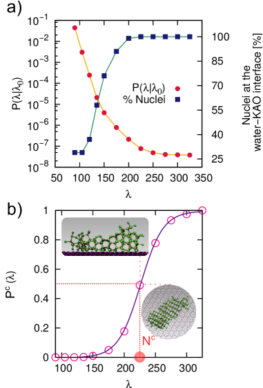
Figure 1: a) Calculated growth probability $P(\lambda|\lambda_{0})$ and fraction of ice nuclei sitting on top of the kaolinite (001) hydroxylated surface as a function of $\lambda$. b) Committor probability $P^{C}(\lambda)$ as a function of $\lambda$. The value of $P^{C}(\lambda)$=0.5, corresponds to the critical nucleus size $N^{C}$=225. A typical ice nucleus of critical size is shown in the insets.

In order to compare our results with the homogeneous data from Ref. 5, we have performed FFS simulations at the same temperature T=230 K, corresponding for the TIP4P/Ice model to $\Delta T$=42 K. The calculated growth probability $P(\lambda|\lambda_{0})$ as a function of $\lambda$ is reported in Fig. 1a. In contrast with the transition probability for homogeneous nucleation reported in Ref. 5, we do not observe any inflection region, i.e. a regime for which the $P(\lambda|\lambda_{0})$ decreases sharply ($P(\lambda_{i}|\lambda_{i-1})<P(\lambda_{j}|\lambda_{j-1})$ for $i<j$). This inflection is because in the early stages of homogeneous nucleation the largest nuclei are mostly made of hexagonal ice ($I_{h}$), which leads to rather aspherical nuclei that are very unlikely to survive and reach the later parts of the nucleation pathway. Within the inflection region the nuclei contain a substantial fraction of cubic ice ($I_{c}$). It seems that in forming this polytype the nuclei are able to adopt a more spherical shape and that this is essential for ultimately growing toward the critical nucleus size. In contrast, within this heterogeneous case, the presence of the surface allows this process of forming spherical $I_{c}$-rich crystallites to be bypassed. Here, nucleation proceeds exclusively heterogeneously at the kaolinite-water interface. During the early stages of the process the fraction of ice nuclei on the surface (as defined in the SI) is only around 25%, as shown in Fig. 1a, since at this strong $\Delta T$ natural fluctuations toward the ice phase are abundant and homogeneously distributed throughout the liquid. However, as nucleation proceeds the nuclei within the bulk of the liquid slab become less favorable, until only nuclei at the water-kaolinite interface survive. From this evidence alone one can conclude that at this temperature kaolinite substantially promotes the formation of ice via heterogeneous nucleation.

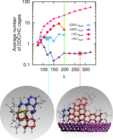
Figure 2: Average number of Double-Diamond Cages $\langle DDC\rangle_{Bulk}$ and Hexagonal Cages $\langle HC\rangle_{Bulk}$ within the largest ice nuclei (identified according to the order parameter $\lambda$) in the bulk of the liquid slab only as a function of $\lambda$ (nuclei in the bulk disappear beyond the value of $\lambda$ marked by the vertical green line). Averages for the largest ice nuclei sitting on top of the kaolinite (001) hydroxylated surface ($\langle DDC\rangle_{Surf}$ and $\langle HC\rangle_{Surf}$) are also reported. The insets depict DDC and HC within an ice nucleus in the bulk at the early stages of nucleation (left) and a post-critical ice nucleus at the water-clay surface (right). Oxygen atoms belonging to the largest ice nucleus (hydrogens not shown) are depicted in blue (DDC), red (HC) and yellow (both DDC and HC). Atoms belonging to the largest ice nucleus but not involved in any DDC or HC are shown in gray.

Our FFS simulation results in a heterogeneous ice nucleation rate of $J_{Hetero}$=$10^{26\pm 2}$ s^-1m^-3, which can be compared with the homogeneous nucleation rate of $J_{Homo}$=$10^{5.9299\pm 0.6538}$ s^-1m^-3 reported in Ref. 5. The hydroxylated (001) surface of kaolinite thus enhances the homogeneous ice nucleation rate by about twenty orders of magnitude at $\Delta T$=42 K. This spectacular boost is similar to that reported for simulations of heterogeneous ice nucleation on graphitic surfaces Cabriolu and Li (2015) and on Lennard-Jones crystals Fitzner et al. (2015) at similar $\Delta T$ using the coarse grained mW model.

An estimate of the critical nucleus size $N^{C}$ can be obtained directly from the crossing probabilities assuming that $\lambda$ is a good reaction coordinate for the nucleation process Haji-Akbari and Debenedetti (2015). In this scenario $N^{C}$ is the value for which the committor probability $P^{C}(\lambda)$ for the nuclei to proceed towards the ice phase instead of shrinking into the liquid is equal to 0.5. As shown in Fig. 1b, $P^{C}(\lambda)$=0.5 corresponds in our case to a critical nucleus of 225 $\pm$ 25 water molecules. The estimate of the homogeneous critical nucleus size, obtained by means of the same approximate approach employed here, is $N^{C}$=500 $\pm$ 30 water molecules (as obtained by using the definition of $\lambda$ employed in this work, see SI), more than two times larger than our estimate for the heterogeneous case.

At this supercooling, homogeneous water nucleates into stacking disordered ice (a mixture of $I_{h}$ and $I_{c}$) Moore and Molinero (2011); Hansen et al. (2008); Malkin et al. (2014). However, the presence of the clay leads to a very different outcome. To analyze the competition between $I_{h}$ and $I_{c}$ we have adopted the topological criterion introduced in Ref. 5 (see SI), pinpointing the building blocks of $I_{c}$ (Double-Diamond Cages, DDC) and $I_{h}$ (Hexagonal Cages, HC) within the largest ice nuclei. The results are summarized in Fig. 2: for ice nuclei in the bulk, a slightly larger fraction of HC with respect to DDC develops until they disappear because of the dominance of the much more favorable nuclei at the surface. In contrast, nuclei at the surface contain a large fraction of HC from the earliest stages of the nucleation, and they exclusively expose the prism face of $I_{h}$ to the hexagonal arrangement of hydroxyl groups of the clay. This is consistent with what has been suggested previously by classical MD simulations Cox et al. (2014); Zielke et al. (2016), and demonstrates that at this supercooling heterogeneous nucleation takes place solely via the hexagonal ice polytype, in contrast with homogeneous nucleation. Experimental evidence Malkin et al. (2014) suggests that stacking disordered ice on kaolinite is likely to appear after the nucleation process due to the kinetics of crystal growth and the presence of surfaces other than the hydroxylated (001).

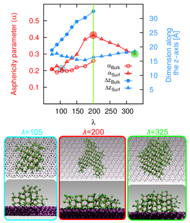
Figure 3: Asphericity parameter $\alpha$ and spatial extent of the ice nuclei along the direction normal to the clay slab $\Delta z$ as a function of $\lambda$ for ice nuclei in the bulk ($\alpha_{Bulk}$ and $\Delta z_{Bulk}$). Nuclei in the bulk disappear beyond the value of $\lambda$ marked by the vertical green line. Averages within the ice nuclei sitting on top of the kaolinite (001) hydroxylated surface ($\alpha_{Surf}$ and $\Delta z_{Surf}$) are also reported. The insets correspond to typical ice nuclei containing about 105, 200 and 325 (from left to right) water molecules.

In the homogeneous case, critical nuclei tend to be rather spherical even at this strong supercooling Haji-Akbari and Debenedetti (2015). However, we see a very different behavior here. This is illustrated in Fig. 3, where we show as a function of $\lambda$ the asphericity parameter $\alpha$ (which is equal to zero for spherical objects and one for an infinitely elongated rod), for nuclei in the bulk and at the surface. Note that heterogeneous CNT predicts (on flat surfaces) critical nuclei in the form of spherical caps, the exact shape of which is dictated by the contact angle $\theta_{Ice,Surf}$ between the nuclei and the surface Cabriolu and Li (2015). For instance, $\alpha$=0.094 for a pristine hemispherical cap, corresponding to $\theta_{Ice,Surf}$=90°. Also reported in Fig. 3 is the spatial extent $\Delta z$ of the nuclei along the direction normal to the slab (the exact definitions of $\alpha$ and $\Delta z$ are provided in the SI). Nuclei within the bulk tend to be rather spherical. A small increase in the asphericity is observed right before these nuclei disappear and are replaced with nuclei at the surface. This regime, in which the nuclei in the bulk grow substantially and become less spherical, possibly corresponds to the onset of the inflection region observed within the homogeneous case. However, here nucleation is dominated by the surface. While nuclei at the surface are initially quite similar to spherical caps, they tend to grow by expanding at the water-kaolinite interface because of the favorable templating effect of the hydroxyl groups, which favors the formation of the prism face of $I_{h}$ Cox et al. (2014). This can clearly be seen by looking at the substantial increase in $\alpha$ for the nuclei at the surface, which is accompanied by a slight drop in $\Delta z$ corresponding to an expansion of the nuclei in two dimensions. Once the nuclei have overcome the critical nucleus size, they tend to return to a more isotropic and compact form, while accumulating new ice layers along the normal to the surface. We note that due to the strong two-dimensional nature of the critical ice nuclei, special care has to be taken to avoid finite size effects. We have therefore used a simulation box with lateral dimensions of the order of 60 Å, which is large enough to prevent interactions between the ice nuclei and their periodic images (as discussed in the SI).

The fact that the system reaches the critical nucleus size by expanding chiefly in two dimensions is in sharp contrast with the heterogeneous nucleation picture predicated by CNT. Hence the question arises: Is CNT able to describe heterogeneous ice nucleation on a complex substrate at this strong supercooling? Strikingly, the answer is yes. In order to show this, we compare the shape factor for heterogeneous nucleation $\mathcal{F}_{S}=\Delta G^{C}_{Hetero}/\Delta G^{C}_{Homo}$, customarily used in CNT Sear (2007) to quantify the net effect of the surface on the free energy barrier for nucleation $\Delta G^{C}$, with the volumetric factor $\mathcal{F}_{V}=N^{C}_{Hetero}/N^{C}_{Homo}$. Details of this comparison are included in the SI. Note that while different, equally valid ways of defining an ice-like cluster can lead to different values of $N^{C}$, there is no ambiguity in the estimate of $\mathcal{F}_{S}$ and $\mathcal{F}_{V}$ as long as the same order parameter is used to define both $N^{C}_{Homo}$ and $N^{C}_{Hetero}$. Thus, we obtain $\mathcal{F}_{S}=0.4\pm 0.1$, in very good agreement with $\mathcal{F}_{V}=0.45\pm 0.08$. Heterogeneous CNT has already proven to be reliable in describing the crystallization of ice on graphitic surfaces Cabriolu and Li (2015), a scenario very different from ice formation on kaolinite. In fact, while the size of the critical clusters reported in Ref. 11 is similar to what has been obtained here (few hundreds of water molecules), critical ice nuclei of mW water on graphitic surfaces are shaped as spherical caps, in line with CNT assumptions. This is due to the fairly weak interaction between water and carbonaceous surfaces Lupi, Hudait, and Molinero (2014), which results in a weak wetting of the ice phase on the substrate. In contrast, our results show that ice nuclei on kaolinite tend to wet substantially the substrate, leading to shapes very different from spherical caps. In this regime, where the nuclei are small and the ice-kaolinite contact angle $\theta_{Ice,Surf}$ is also small, line tension at the water-ice-kaolinite interface could introduce a mismatch between $\mathcal{F}_{S}$ and $\mathcal{F}_{V}$ (see e.g. Refs. 37; 38). However, this is not the case, as CNT holds quantitatively for the formation of ice on kaolinite even at the strong supercooling probed in this work.

The value of $J_{Homo}$ reported in Ref. 5 is about eleven orders of magnitude smaller than the experimental value extrapolated from Ref. 39. In addition, at the strong supercooling of $\Delta T$=42 K no direct measures of $J_{Hetero}$ exist for kaolinite (nor indeed for the homogeneous case), as pure water freezes homogeneously at $T<\Delta T\sim 38K$. Consequently, extrapolations are necessary, leading to experimental uncertainties as large as six orders of magnitude Sosso et al. (2016). Nonetheless, our $\mathcal{F}_{S}$ quantifies the $relative$ ice nucleation ability of kaolinite with respect to the homogeneous case, which can thus be compared with experimental values. Estimates of $\mathcal{F}_{S}$ from measurements of ice formation on kaolinite particles can vary from 0.23 to 0.69 according to the interpretation of the experimental data Ickes, Welti, and Lohmann (2016), and the seminal work of Murray Murray et al. (2011) suggests a value of 0.11 for the exclusive formation of $I_{h}$ observed in this work. The variability of these experimental results stems mainly from the diversity of the kaolinite samples (in terms of e.g. shape, purity and surfaces exposed, the latter still largely unknown) and the difficulty to interpret the experimental data using heterogeneous CNT, for which tiny changes in quantities such as the free energy difference between water and ice lead to substantial discrepancies Haji-Akbari and Debenedetti (2015). To date, experiments have to deal with populations of uneven particles and different nucleation sites. Here we provide a value of $\mathcal{F}_{S}$ for a perfectly flat, defect-free (001) hydroxylated surface of kaolinite, in the hope to aid the experimental investigation of well-defined, clean kaolinite substrates in the near future. We also note that our simulations of crystal nucleation are the very edge of what molecular dynamics can presently achieve. However, there is still room for improvement: for instance, heterogeneous ice formation can be affected by the presence of electric fields Ehre et al. (2010); Yan and Patey (2011), and similarly, water dissociation is common on many reactive surfaces Carrasco, Hodgson, and Michaelides (2012); these effects cannot be accounted for at present with the traditional force fields employed here.

In summary, we have calculated the heterogeneous ice nucleation rate for a fully atomistic water model on a prototypical clay mineral of great importance to environmental science. We have demonstrated that the hydroxylated (001) surface of kaolinite boosts ice formation by twenty orders of magnitude with respect to homogeneous nucleation at the same supercooling. We have found that this particular kaolinite surface promotes the nucleation of the hexagonal ice polytype, which forms thanks to the interaction of the prism face with the templating arrangements of hydroxyl groups at the clay interface. We have also found that ice nuclei tend to expand on the clay surface in two dimensions until they reach the critical nucleus size. This is in contrast with the predictions of CNT, which however holds quantitatively for ice formation on kaolinite even at this strong supercooling. Finally, we provide a value of the heterogeneous shape factor for the defect-free surface considered here, in the first attempt to bring simulations of heterogeneous ice nucleation a step closer to experiments. It remains to be investigated to what extent different surface morphologies can in general affect nucleation rates or alter the ice polytypes which form.

SUPPORTING INFORMATION

We provide supporting information on the calculation of the heterogeneous ice nucleation rate on the kaolinite (001) hydroxylated surface. The computational geometry is specified together with the details of the molecular dynamics simulations used in this work. Moreover, we discuss the choice of the order parameter we have employed within the forward flux sampling calculations, and we provide additional information about the implementation of the algorithm and the results obtained at each stage of the latter. A brief discussion about heterogeneous classical nucleation theory is also presented together with the technical details of the topological criteria used to characterized the ice nuclei and a discussion about finite size effects.

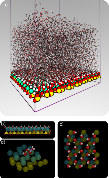
Fig. S S1: a) The simulation cell used in this work. A film of liquid water about 40 Å   thick is in contact with a single slab of kaolinite, cleaved along the (001) plane. This slab geometry is thus characterized by two interfaces: the water-kaolinite interface and the water-vacuum interface. The dimension of the simulation box along the normal to the slab is extended up to 150 Å. Water molecules are depicted as sticks, while atoms within the kaolinite slab as balls. Red, white, light blue and yellow atoms correspond to oxygen, hydrogen, aluminum and silicon atoms respectively. b) (side view) The layered structure of the kaolinite slab: yellow tetrahedra and light blue octahedra represent the tetrahedral silica sheet and the octahedral alumina sheet, terminated with hydroxyl groups, respectively. c) (top view) A small portion of the kaolinite slab depicting the hexagonal arrangement of the hydroxyl groups exposed. d) Sketch of the amphoteric character of the hydroxylated (001) face of kaolinite: the hydroxyl groups on top can either donate or accept an hydrogen bond from e.g. water molecules at the water-clay interface.

Computational Geometry

The computational setup we have used is depicted in Fig. S1a. A single layer of kaolinite, cleaved along the (001) plane (perpendicular to the normal to the slab) was prepared by starting from the experimental cell parameters and lattice positions Bish (1993). Specifically, a kaolinite bulk system made of two identical slabs was cleaved along the (001) plane. The triclinc symmetry of the system (space group $C1$) was modified by setting the $\alpha$ and $\gamma$ angles (experimentally equal to 91.926 and 89.797 degrees respectively Bish (1993)) to 90 degrees in order to make the cell orthorombic. We explicitly verified that this modification does not introduce any structural change within the clay. The final slab has in-plane dimensions of 61.84 and 71.54 Å, corresponding to a 12 by 8 supercell. We positioned 6144 water molecules randomly atop this kaolinite slab at the density of the TIP4P/Ice model Abascal et al. (2005) at 300 K, and expanded the dimension of the simulation cell along the normal to the slab to 150 Å. This setup allows for a physically meaningful equilibration of the water at the density of interest at a given temperature, but suffers from two distinct drawbacks: i) the kaolinite slab possesses a net dipole moment which is not compensated throughout the simulation cell and ii) the presence of the water-vacuum interface can alter the structure and the dynamics of the liquid film. However, we have verified that compensating the dipole moment by means of a mirror slab does not affect our simulations, as we have been able to replicate the results of Ref. 3 independently of the computational geometry. Furthermore, the water film is thick enough to allow a bulk-like region to exist in terms of both structure and dynamics. The effect of the water-vacuum interface is therefore negligible. In Fig. S1b we highlight the layered nature of the slab, while in Fig. S1c we zoom in on a portion of the (001) hydroxylated surface and show the hexagonal arrangement of the hydroxyl groups. This arrangement is important as the water can interact with the hydroxyls, so this arrangement is responsible for the templating effect of the clay which serves to promote ice nucleation. The amphoteric nature of the hydroxyl groups at the surface is depicted in Fig. S1d.

Molecular Dynamics Simulations

The CLAY_FF Cygan et al. (2004) force field was used to model the kaolinite slab. We have not included the - optional - angular term (see Ref. 4), as we have verified that it does not affect the structure of the surface. In order to mimic the experimental conditions, we have constrained the system at the experimental lateral dimensions (see above), and have also restrained the positions of the silicon atoms at the bottom of the slab by means of an harmonic potential characterized by a spring constant of 1000 kJ/mol. All the other atoms within the kaolinite slab are unconstrained. We have verified that the thermal expansion of the clay at 230 K ($\sim$ 0.4% with respect to each lateral dimension) does not alter the structure nor the dynamics of the water-kaolinite interface. This setup is thus as close as we can get to the realistic (001) hydroxylated surface within the CLAY_FF model. The interaction between the water molecules have been modeled using the TIP4P/Ice model Abascal et al. (2005), so that our results are consistent with the homogeneous simulations of Ref. 5. The interaction parameters between the clay and the water were obtained using the standard Lorentz-Berthelot mixing rules Lorentz (1881); Berthelot and Hebd (1898). Extreme care must be taken in order to correctly reproduce the structure and the dynamics of the water-clay interface. The Forward Flux Sampling (FFS) simulations reported in this work rely on a massive collection of unbiased Molecular Dynamics (MD) runs, all of which have been performed using the GROMACS package, version 4.6.7. The code was compiled in single-precision, in order to alleviate the huge computational workload needed to converge the FFS algorithm and because we have taken advantage of GPU acceleration, which is not available in the double-precision version. The equations of motions were integrated using a leap-frog integrator with a timestep of 2 fs. The van der Waals (non bonded) interactions were considered up to 10 Å, where a switching function was used to bring them to zero at 12 Å. Electrostatic interactions have been dealt with by means of an Ewald summation up to 14 Å. The NVT ensemble was sampled at 230 K using a stochastic velocity rescaling thermostat Bussi et al. (2007) with a very weak coupling constant of 4 ps in order to avoid temperature gradients throughout the system. The geometry of the water molecules (TIP4P/Ice being a rigid model) was constrained using the SETTLE algorithm Miyamoto and Kollman (1992) while the P_LINCS algorithm Hess et al. (1997) was used to constrain the O-H bonds within the clay. We have verified that these settings reproduce the dynamical properties of water reported in Ref. Haji-Akbari and Debenedetti (2015). The system was equilibrated at 300 K for 10 ns, before being quenched to 230 K over 50 ns. This is the starting point for the calculation of the flux rate discussed in the next section.

Forward Flux Sampling Simulation

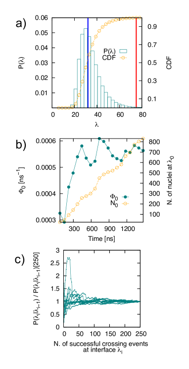
Fig. S S2: a) Probability density distribution for the order parameter $\lambda$ ($P(\lambda)$ left y-axis, boxes) and correspondent cumulative distribution function (CDF, right y-axes, empty circles). The blue and red vertical arrows mark the upper limit of the liquid basin $\lambda_{Liq}$ and the position of $\lambda_{0}$ respectively. b) Flux rate ($\Phi_{0}$, left y-axis, filled circles) and number of direct crossing of the $\lambda_{0}$ interface ($N_{0}$, right y-axis, empty circles) as a function of simulation time. c) Individual crossing probabilities $P(\lambda_{i}|\lambda_{i-1})$ (normalized by their value at N=250) as a function of the number of crossing events.

Order Parameter

The first step in setting up the FFS simulation involved choosing a suitable order parameter $\lambda$. We start by labeling as ice-like any water molecule whose oxygen atom displays a value of $lq^{6}$¿0.45, where $lq^{6}$ is constructed as follows: we first select only those oxygens which are hydrogen-bonded to four other oxygens. For each of the $i-$th atoms of this subset $S_{4HB}$, we calculate the local order parameter:

$$lq^{6}_{i}=\frac{\sum_{j=1}^{N_{S_{4HB}}}\sigma(\mathbf{r}_{ij})\sum_{m=-6}^{6}q^{6*}_{i,m}\cdot q^{6}_{j,m}}{\sum_{j=1}^{N_{S_{4HB}}}\sigma(\mathbf{r}_{ij})}$$ (S1)

where $\sigma(\mathbf{r}_{ij})$ is a switching function tuned so that $\sigma(\mathbf{r}_{ij})$=1 when atom $j$ lies within the first coordination shell of atom $i$ and which is zero otherwise. $q^{6}_{i,m}$ is the Steinhardt vector Steinhardt et al. (1983)

$$q^{6}_{i,m}=\frac{\sum_{j=1}^{N_{S_{4HB}}}\sigma(\mathbf{r}_{ij})Y_{6m}(\mathbf{r}_{ij})}{\sum_{j=1}^{N_{S_{4HB}}}\sigma(\mathbf{r}_{ij})},$$ (S2)

$Y_{6m}(\mathbf{r}_{ij})$ being one of the 6th order spherical harmonics. We have used 3.2 Å   as the cutoff for $\sigma(\mathbf{r}_{ij})$ to be consistent with Ref. 5. Note that by selecting oxygen atoms within the $S_{4HB}$ subset exclusively we ensure that the hydrogen bond network within the ice nuclei is reasonable. Having identified a set of ice-like water molecules, we pinpoint all the connected clusters of oxygen atoms which: i) belong to the $S_{4HB}$ subset; ii) have a value of $lq^{6}$¿0.45 and; iii) are separated by a distance $\leq$ 3.2 Å. We then select the largest of these clusters (i.e. the one containing the largest number of oxygen atoms or equivalently water molecules). The final step is to find all the surface molecules that are connected to this cluster, as this procedure allows us to account for the diffuse interface between the solid and the liquid. Surface molecules are defined as the water molecules that lie within 3.2 Å   from the molecules in the cluster. The final order parameter $\lambda$ used in this work is thus the number of water molecules within the largest ice-like cluster plus the number of surface molecules. This approach allow us to include ice-like atoms sitting directly on top of the kaolinite surface, which are never labeled as ice-like (and which would thus never be included into the ice nuclei) because they are undercoordinated and because they display a different symmetry to the molecules within bulk water (which in turn leads to different values of $lq^{6}$). Note that the order parameter used in Ref. 5 differs with respect to our formulation in that i) a slightly stricter criterion has been used to label molecules as ice-like, namely $lq^{6}$¿0.5 to be compared with our choice of $lq^{6}$¿0.45; and ii) surface molecules are not included in the largest ice-like nucleus. This means that in order to compare quantitatively our results with those of Ref. 5 in terms of e.g. the size of the critical nucleus, the very same order parameter has to be used. The calculation of the order parameter is performed on the fly during our MD simulations thanks to the flexibility of the PLUMED plugin Tribello et al. (2014) (version 2.2). This code deals chiefly with metadynamics simulations, but can be adapted to a FFS simulation. Note that PLUMED benefits from a fully parallel implementation that flawlessly couples with the GPU-accelerated version of GROMACS, and thus provides a very fast tool for performing FFS simulations. Indeed, while several implementations of FFS are beginning to appear, the main issue preventing wider adoption remains the implementation of the order parameter, which can be as complex as the one used in this work. PLUMED allows a wide range of order parameters to be exploited without the need to re-code them elsewhere.

Converging the Flux Rate and the Individual Crossing Probabilities

In order to calculate the flux rate ${\Phi_{0}}$ we have performed a 1.5 ms long unbiased MD simulation, and subsequently built the probability density distribution for $P(\lambda)$ shown in Fig. S2a. We have thus delimited the liquid basin in terms of the order parameter as $0<\lambda<\lambda_{Liq}=32$, while setting the initial interface for the FFS $\lambda_{0}$=75, corresponding to a value of the cumulative distribution function of $P(\lambda)$ (also reported in Fig. S2a) of 0.99. The flux rate is then computed as the number of direct crossings of $\lambda_{0}$ (i.e. coming from $\lambda<\lambda_{Liq}$) divided by the total simulation time, and as such should flatten as a function of time. Meanwhile, the number of direct crossings should increase linearly with time. The value obtained for ${\Phi_{0}}$ and the number of crossings as a function of time are reported in Fig. S2b. This figure demonstrates that, as previously noted in Ref. 13, long simulation times are needed in order to converge this quantity for inhomogeneous systems. The calculated value of ${\Phi_{0}}$ is 0.00056359 ps^-1, which normalized by the average volume of the water film (189350.2980352 ų) leads to the final value of 3.0$\cdot$10^-9±1 ps^-1 Å^-3. Note that we have chosen to normalize the flux rate by the average volume of the water film instead of by the surface area for the slab. While the latter choice could in principle be thought as more meaningful in the context of heterogeneous nucleation, our objective is to compare our numbers with the homogeneous case, which is why we choose the volume normalization rather than the surface area one. However, it should be noticed that the two different normalizations only introduce a difference of an order of magnitude in the nucleation rate. The number of starting configurations, one for each direct crossing of $\lambda_{0}$, is of the order of eight hundred, providing a comprehensive sampling including ice-like clusters in the bulk of the water film as well as on top of the water surface (albeit the latter represent about 25%).

Converging the individual crossing probabilities $P(\lambda_{i}|\lambda_{i-1})$ required in our case as many as 10,000 trial MD runs for the first few interfaces. The initial velocities for each MD run were randomly initialized consistent with the corresponding Maxwell-Boltzmann distribution at 230 K. In line with the coarse graining approach discussed in Ref. 5, we have decided to compute the value of $\lambda$ on the fly every 4 ps, a frequency far smaller than the relaxation time of the liquid at this temperature (about 0.5 ns) which allows us to neglect meaningless fluctuation on very short timescales. The individual crossing probabilities, normalized by their value after 250 crossing events, are reported in Fig. S2c. Note that at the interfaces corresponding to critical/post-critical ice nuclei a much smaller number (about 500) of trial MD runs have been shot, as for large ice nuclei to get back to the liquid phase simulation times of the order of 10-40 ns are needed, dramatically increasing the computational cost - albeit more and more nuclei proceed to grow as $\lambda$ increases leading to a faster convergence of the crossing probabilities. In fact, crossings for n¿250 are not reported in Fig. S2c as the crossing probabilities are already converged well before n=250 within the last stages of the algorithm. The confidence intervals for each $P(\lambda_{i}|\lambda_{i-1})$ have been computed according to the binomial distribution of the number of successful trial runs collected at $\lambda_{i}$ (see e.g. Ref. Allen et al. (2006)).

Heterogeneous Classical Nucleation Theory

Within the framework of classical nucleation theory, the homogeneous rate of nucleation $J_{Homo}$ can be written as Sear (2007); Kalikmanov (2013):

$$J_{Homo}=A_{Homo}\cdot e^{-\frac{\Delta G^{*}_{Homo}}{k_{B}T}}$$ (S3)

where $A_{Homo}$ is a kinetic prefactor, $\Delta G^{*}_{Homo}$ is the height of the free energy barrier for nucleation and $k_{B}$ is the Boltzmann constant. On the other hand, the heterogeneous rate of nucleation $J_{Hetero}$ can be written as Sear (2007); Kalikmanov (2013):

$$J_{Hetero}=A_{Hetero}\cdot e^{-\frac{\mathcal{F}_{S}\cdot\Delta G^{*}_{Homo}}{k_{B}T}}$$ (S4)

where $A_{Hetero}$ is a kinetic prefactor which in principle can differ from $A_{Homo}$ and $\mathcal{F}_{S}$ is a shape factor, or potency factor, which embeds the effectiveness of the substrate to promote nucleation. The value of $\mathcal{F}_{S}$ ranges from one (the surface does not contribute at all in lowering the free energy barrier for nucleation) to 0 (the nucleation proceeds in a barrierless fashion). By taking the ratio $\frac{J_{Hetero}}{J_{Homo}}$ and assuming that $A_{Hetero}=A_{Homo}$ (which is in many cases a perfectly reasonable assumption, see e.g. Refs. 17; 18; 19), one can write the shape factor for heterogeneous nucleation as:

$$\mathcal{F}_{S}=1-\left[\frac{k_{B}T}{\Delta G^{*}_{Homo}}\cdot\ln\left(\frac{J_{Hetero}}{J_{Homo}}\right)\right]$$ (S5)

The value of $\Delta G^{*}_{Homo}=\frac{1}{2}|\Delta\mu_{sl}|N^{C}_{Homo}$ is 80$\pm$ 5 $k_{B}T$, obtained from Ref. 5 by using the definition of $\lambda$ we have employed here (thus using a slighlty different $lq_{i}^{6}$ cutoff and including surface molecules, see Eq. S1) - which accounts for an homogeneous critical nucleus size of 500 $\pm$ 30 water molecules and makes a direct comparison possible. Inserting this value into the expression above leads to a shape factor of $0.4\pm 0.1$.

Double-Diamond and Hexagonal Cages

Double-Diamond (DDC) and Hexagonal cages (HC) are the building blocks of cubic and hexagonal ice respectively. We have identified water molecules involved in DDC and/or HC within the largest ice nucleus in the system (defined according to the order parameter $\lambda$, see Eqs. 1 and 2) following the topological criteria detailed in Ref. 5. The first step in order to locate DDC and HC is the construction of the ring network of the oxygen atoms belonging to each water molecule. In this work, we have obtained all the six-atom rings needed to build DDC and HC using King’s shortest path criterion King (1967); Franzblau (1991) as implemented in the R.I.N.G.S. code Le Roux and Jund (2010). The same distance cutoff of 3.2 Å   used for the construction of the order parameter $\lambda$ has been employed to determine the nearest neighbors of each oxygen atom. The same algorithm described in Ref. 5 has subsequently been used to determine DDC and HC.

Asphericity Parameter

Many different choices are available to quantify the asphericity of clusters of molecules. We have considered the gyration radius as well as the $\alpha$ ( $\Delta$ in Ref. 23) and $S$ asphericity parameters reported in Ref. 23. All of these quantities provided the same qualitative picture, so we have chosen to report the asphericity trends for $\alpha$ only, the latter being defined as:

$$\alpha=\frac{3}{2(tr\mathcal{T})^{2}}\sum_{i=1}^{3}(\mu_{i}-\bar{\mu})^{2}$$ (S6)

where $\mu_{i}$ are the three eigenvalues of the inertia tensor $\mathcal{T}$ for a given cluster, and $\bar{\mu}=\frac{tr\mathcal{T}}{3}=\frac{\sum_{i=1}^{3}(\mu_{i})}{3}$

Spatial extent $\Delta z$

The spatial extent $\Delta z$ for a given ice nucleus has been calculated as the difference between the minimum and maximum values of the z- components of the position vector of all the oxygens belonging to the nucleus. As the direction normal to the kaolinite slab coincides to the z-axis of our simulation box, $\Delta z$ provides a qualitative indication of the number of ice layers in the nuclei. Ice nuclei are defined to be on top of the kaolinite surface ($Surf$, see main text) if the minimum value of the z- components of the position vector of all the oxygens belonging to the nucleus is ¡ 15.0 Å, which correspond to the position of the main peak in the density profile of the water film along the z-axis. If this is not the case, the ice nuclei are considered to sit in the bulk of the water film ($Bulk$, see main text).

Avoiding Finite Size Effects

Special care has to be taken when dealing with atomistic simulations of crystal nucleation from the liquid phase. Specifically, the presence of periodic boundary conditions can introduce significant finite effects, most notably spurious interactions between the crystalline nuclei and their periodic images. This artefact results in nonphysically large nucleation rates and/or crystal growth speeds. In this work we have considered simulation boxes with lateral dimensions of the order of 60 Å, which is sufficient to ensure that finite size effects do not affect our results. We also measured the distance between the ice nuclei and their periodic images using the average set-set distance $d(A,B)$, which is defined as:

$$d(A,B)=\text{inf}\lim_{x\in A,y\in B}|\mathbf{x}-\mathbf{y}|$$ (S7)

where $x$ and $y$ are the position vectors of each oxygen atoms belonging to the largest ice nucleus (defined according to the order parameter $\lambda$) $A$ and its first periodic image $B$ respectively. At the FFS interface closest to the critical nucleus size ($\lambda$=225), $d(A,B)$=20$\pm$6Å, and even at the last FFS interface we have considered ($\lambda$=325) the ice nuclei are still quite far away from their periodic images, $d(A,B)$ being 15$\pm$7Å, which is of the order of 1/4 of the lateral dimension of the simulation box.

References

- Tam et al. (2009) R. Y. Tam, C. N. Rowley, I. Petrov, T. Zhang, N. A. Afagh, T. K. Woo, and R. N. Ben, J. Am. Chem. Soc. 131, 15745 (2009).
- Bolton and Pettersson (2001) K. Bolton and J. B. C. Pettersson, J. Am. Chem. Soc. 123, 7360 (2001).
- Tang, Cziczo, and Grassian (2016) M. Tang, D. J. Cziczo, and V. H. Grassian, Chem. Rev. 116, 4205 (2016).
- Bartels-Rausch et al. (2012) T. Bartels-Rausch, V. Bergeron, J. H. E. Cartwright, R. Escribano, J. L. Finney, H. Grothe, P. J. Gutiérrez, J. Haapala, W. F. Kuhs, J. B. C. Pettersson, S. D. Price, C. I. Sainz-Díaz, D. J. Stokes, G. Strazzulla, E. S. Thomson, H. Trinks, and N. Uras-Aytemiz, Rev. Mod. Phys. 84, 885 (2012).
- Pirzadeh and Kusalik (2013) P. Pirzadeh and P. G. Kusalik, J. Am. Chem. Soc. 135, 7278 (2013).
- Murray et al. (2012) B. J. Murray, D. O’Sullivan, J. D. Atkinson, and M. E. Webb, Chem. Soc. Rev. 41, 6519 (2012).
- Lupi, Hudait, and Molinero (2014) L. Lupi, A. Hudait, and V. Molinero, J. Am. Chem. Soc. 136, 3156 (2014).
- O’Sullivan et al. (2015) D. O’Sullivan, B. J. Murray, J. F. Ross, T. F. Whale, H. C. Price, J. D. Atkinson, N. S. Umo, and M. E. Webb, Sci. Rep. 5, 1 (2015).
- Eastwood et al. (2008) M. L. Eastwood, S. Cremel, C. Gehrke, E. Girard, and A. K. Bertram, J. Geophys. Res. 113, D22203 (2008).
- Fitzner et al. (2015) M. Fitzner, G. C. Sosso, S. J. Cox, and A. Michaelides, J. Am. Chem. Soc. 137, 13658 (2015).
- Cabriolu and Li (2015) R. Cabriolu and T. Li, Phys. Rev. E 91, 052402 (2015).
- Zimmermann et al. (2008) F. Zimmermann, S. Weinbruch, L. Schiütz, H. Hofmann, M. Ebert, K. Kandler, and A. Worringen, J. Geophys. Res. 113, D23204 (2008).
- Murray et al. (2011) B. J. Murray, S. L. Broadley, T. W. Wilson, J. D. Atkinson, and R. H. Wills, Atmos. Chem. Phys. 11, 4191 (2011).
- Tobo et al. (2012) Y. Tobo, P. J. DeMott, M. Raddatz, D. Niedermeier, S. Hartmann, S. M. Kreidenweis, F. Stratmann, and H. Wex, Geophys. Res. Lett. 39, L19803 (2012).
- Welti et al. (2013) A. Welti, Z. A. Kanji, F. Lüöd, O. Stetzer, and U. Lohmann, J. Atmos. Sci. 71, 16 (2013).
- Wex et al. (2014) H. Wex, P. J. DeMott, Y. Tobo, S. Hartmann, M. Rösch, T. Clauss, L. Tomsche, D. Niedermeier, and F. Stratmann, Atmos. Chem. Phys. 14, 5529 (2014).
- Hu and Michaelides (2010) X. L. Hu and A. Michaelides, Surf. Sci. 604, 111 (2010).
- Tunega, Gerzabek, and Lischka (2004) D. Tunega, M. H. Gerzabek, and H. Lischka, J. Phys. Chem. B 108, 5930 (2004).
- Cox et al. (2014) S. J. Cox, Z. Raza, S. M. Kathmann, B. Slater, and A. Michaelides, Farad. Discuss. 167, 389 (2014).
- Zielke, Bertram, and Patey (2016) S. A. Zielke, A. K. Bertram, and G. N. Patey, J. Phys. Chem. B 120, 1726 (2016).
- Sanz et al. (2013) E. Sanz, C. Vega, J. R. Espinosa, R. Caballero-Bernal, J. L. F. Abascal, and C. Valeriani, J. Am. Chem. Soc. 135, 15008 (2013).
- Haji-Akbari and Debenedetti (2015) A. Haji-Akbari and P. G. Debenedetti, Proc. Natl. Acad. Sci. 112, 10582 (2015).
- Pruppacher and Klett (1997) H. R. Pruppacher and J. D. Klett, Microphysics Of Clouds And Precipitation (Springer Science & Business Media, 1997).
- Abascal et al. (2005) J. L. F. Abascal, E. Sanz, R. G. Fernandez, and C. Vega, J. Chem. Phys. 122, 234511 (2005).
- Hu and Michaelides (2008) X. L. Hu and A. Michaelides, Surf. Sci. 602, 960 (2008).
- Allen, Valeriani, and Rein ten Wolde (2009) R. J. Allen, C. Valeriani, and P. Rein ten Wolde, J. Phys. Cond. Matt. 21, 463102 (2009).
- Li et al. (2011) T. Li, D. Donadio, G. Russo, and G. Galli, Phys. Chem. Chem. Phys. 13, 19807 (2011).
- Li, Donadio, and Galli (2013) T. Li, D. Donadio, and G. Galli, Nat. Comm. 4, 1887 (2013).
- Valeriani, Sanz, and Frenkel (2005) C. Valeriani, E. Sanz, and D. Frenkel, J. Chem. Phys. 122, 194501 (2005).
- Wang, Valeriani, and Frenkel (2009) Z.-J. Wang, C. Valeriani, and D. Frenkel, J. Phys. Chem. B 113, 3776 (2009).
- Bi and Li (2014) Y. Bi and T. Li, J. Phys. Chem. B 118, 13324 (2014).
- Gianetti et al. (2016) M. M. Gianetti, A. Haji-Akbari, M. P. Longinotti, and P. G. Debenedetti, Phys. Chem. Chem. Phys. 18, 4102 (2016).
- Moore and Molinero (2011) E. B. Moore and V. Molinero, Phys. Chem. Chem. Phys. 13, 20008 (2011).
- Hansen et al. (2008) T. C. Hansen, M. M. Koza, P. Lindner, and W. F. Kuhs, J. Phys. Cond. Matt. 20, 285105 (2008).
- Malkin et al. (2014) T. L. Malkin, B. J. Murray, C. G. Salzmann, V. Molinero, S. J. Pickering, and T. F. Whale, Phys. Chem. Chem. Phys. 17, 60 (2014).
- Sear (2007) R. P. Sear, J. Phys. Cond. Matt. 19, 033101 (2007).
- Auer and Frenkel (2003) S. Auer and D. Frenkel, Phys. Rev. Lett. 91, 015703 (2003).
- Winter, Virnau, and Binder (2009) D. Winter, P. Virnau, and K. Binder, Phys. Rev. Lett. 103, 225703 (2009).
- Sellberg et al. (2014) J. A. Sellberg, C. Huang, T. A. McQueen, N. D. Loh, H. Laksmono, D. Schlesinger, R. G. Sierra, D. Nordlund, C. Y. Hampton, D. Starodub, D. P. DePonte, M. Beye, C. Chen, A. V. Martin, A. Barty, K. T. Wikfeldt, T. M. Weiss, C. Caronna, J. Feldkamp, L. B. Skinner, M. M. Seibert, M. Messerschmidt, G. J. Williams, S. Boutet, L. G. M. Pettersson, M. J. Bogan, and A. Nilsson, Nature 510, 381 (2014).
- Sosso et al. (2016) G. Sosso, J. Chen, S. Cox, M. Fitzner, P. Pedevilla, A. Zen, and A. Michaelides, Chem. Rev. , DOI: 10.1021/acs.chemrev.5b00744 (2016).
- Ickes, Welti, and Lohmann (2016) L. Ickes, A. Welti, and U. Lohmann, Atm. Chem. Phys. Discuss. 16, 1 (2016).
- Ehre et al. (2010) D. Ehre, E. Lavert, M. Lahav, and I. Lubomirsky, Science 327, 672 (2010).
- Yan and Patey (2011) J. Y. Yan and G. N. Patey, J. Phys. Chem. Letters 2, 2555 (2011).
- Carrasco, Hodgson, and Michaelides (2012) J. Carrasco, A. Hodgson, and A. Michaelides, Nat. Mat. 11, 667 (2012).

References

- Bish (1993) Bish, D. L. Clays and Clay Minerals 1993, 41, 738–744.
- Abascal et al. (2005) Abascal, J. L. F.; Sanz, E.; Fernandez, R. G.; Vega, C. The Journal of Chemical Physics 2005, 122, 234511.
- Zielke et al. (2016) Zielke, S. A.; Bertram, A. K.; Patey, G. N. J. Phys. Chem. B 2016, 120, 1726–1734.
- Cygan et al. (2004) Cygan, R. T.; Liang, J.-J.; Kalinichev, A. G. The Journal of Physical Chemistry B 2004, 108, 1255–1266.
- Haji-Akbari and Debenedetti (2015) Haji-Akbari, A.; Debenedetti, P. G. Proceedings of the National Academy of Sciences 2015, 201509267.
- Lorentz (1881) Lorentz, H. A. Annalen der Physik 1881, 248, 127–136.
- Berthelot and Hebd (1898) Berthelot, D.; Hebd, C. R. Seances De L’ Academie Des Sciences. 1898.
- Bussi et al. (2007) Bussi, G.; Donadio, D.; Parrinello, M. The Journal of Chemical Physics 2007, 126, 014101.
- Miyamoto and Kollman (1992) Miyamoto, S.; Kollman, P. A. Journal of Computational Chemistry 1992, 13, 952–962.
- Hess et al. (1997) Hess, B.; Bekker, H.; Berendsen, H. J. C.; Fraaije, J. G. E. M. Journal of Computational Chemistry 1997, 18, 1463–1472.
- Steinhardt et al. (1983) Steinhardt, P. J.; Nelson, D. R.; Ronchetti, M. Physical Review B 1983, 28, 784–805.
- Tribello et al. (2014) Tribello, G. A.; Bonomi, M.; Branduardi, D.; Camilloni, C.; Bussi, G. Computer Physics Communications 2014, 185, 604–613.
- Bi and Li (2014) Bi, Y.; Li, T. The Journal of Physical Chemistry B 2014, 118, 13324–13332.
- Allen et al. (2006) Allen, R. J.; Frenkel, D.; Wolde, P. R. t. The Journal of Chemical Physics 2006, 124, 194111.
- Sear (2007) Sear, R. P. Journal of Physics: Condensed Matter 2007, 19, 033101.
- Kalikmanov (2013) Kalikmanov, V. Nucleation Theory; Lecture Notes in Physics; Springer Netherlands: Dordrecht, 2013; Vol. 860.
- Li et al. (2011) Li, T.; Donadio, D.; Russo, G.; Galli, G. Physical Chemistry Chemical Physics 2011, 13, 19807–19813.
- Li et al. (2013) Li, T.; Donadio, D.; Galli, G. Nature Communications 2013, 4, 1887.
- Gianetti et al. (2016) Gianetti, M. M.; Haji-Akbari, A.; Longinotti, M. P.; Debenedetti, P. G. Physical Chemistry Chemical Physics 2016, 18, 4102–4111.
- King (1967) King, S. V. Nature 1967, 213, 1112–1113.
- Franzblau (1991) Franzblau, D. S. Physical Review B 1991, 44, 4925–4930.
- Le Roux and Jund (2010) Le Roux, S.; Jund, P. Computational Materials Science 2010, 49, 70–83.
- Rawat and Biswas (2011) Rawat, N.; Biswas, P. Physical Chemistry Chemical Physics 2011, 13, 9632–9643.